Hierarchical Fusion Method for SAR-Based Coastal Bathymetric Inversion in Short-Period Wave-Dominated Areas: A Case Study of the Wengtian Coast, Hainan Island

Highlights

What are the main findings?

• In short-period wave-dominated areas, SAR-based bathymetric inversion suffers from limited accuracy and stability.
• A hierarchical fusion method for SAR-based coastal bathymetric inversion is proposed, specifically designed for short-period wave-dominated areas.

What are the implications of the main findings?

• An effective solution is provided for robust and accurate coastal bathymetric inversion.
• The potential of multi-temporal SAR-based bathymetric inversion in short-period wave-dominated coastal waters is demonstrated.

Abstract

Coastal bathymetric information is essential for marine engineering, navigation safety, and coastal management. Coastal bathymetric inversion based on wave characteristics extracted from synthetic aperture radar (SAR) images is a widely used technique. Existing studies that apply this method have mostly focused on long-period wave-dominated areas. However, in short-period wave-dominated areas, this method suffers from large errors and poor stability, limiting its practical application. To address this problem, this study proposes a hierarchical fusion method for SAR-based coastal bathymetric inversion in short-period wave-dominated areas. The proposed method significantly reduces bathymetric inversion errors by hierarchically fusing multi-angle wavelength estimation results and multi-temporal SAR bathymetry inversion results, thereby achieving more robust underwater topography mapping. A validation experiment was conducted on the Wengtian coast, Hainan Island. Compared with the best single-temporal inversion results, the proposed method reduces the MAE by 19.5% and the RMSE by 23.5%. Finally, the effects of the dispersion relation and the selection of the fusion strategy on the bathymetric inversion results are discussed. These results show that the proposed method significantly improves bathymetric inversion accuracy in short-period wave-dominated areas.

1. Introduction

Coastal bathymetry inversion provides important guidance for human development activities, such as maritime transportation, marine fisheries, and offshore oil and gas exploration and development [1,2]. Synthetic aperture radar (SAR) has been widely applied to coastal bathymetric mapping, owing to its all-day, all-weather, and high-resolution Earth observation capability [3,4,5,6]. A common SAR-based coastal bathymetric inversion method is based on wave characteristic variations, which rely on the interaction between underwater topography and ocean waves [7,8,9,10,11,12]. As ocean waves propagate from deep water to shallow water, they exhibit phenomena such as shoaling and refraction [13,14,15], accompanied by changes in wave parameters. Therefore, coastal bathymetry can be inverted by obtaining wave parameters and solving the dispersion relation.

When retrieving coastal bathymetry from wave characteristics, wave period is one of the key factors affecting inversion accuracy. Boccia et al. [16] analyzed the linear dispersion relation. For the same water depth, a shorter wave period corresponds to a steeper slope of the dispersion relation curve. This in turn leads to higher uncertainty in bathymetric inversion. Pereira et al. [10] evaluated the effect of wavelength variation on the relative error of bathymetric inversion under different wave periods. The results showed that under short-period wave conditions, the relative error introduced by wavelength variation was larger. These studies consistently show that a shorter wave period is associated with larger bathymetric inversion errors. To quantitatively characterize this impact, Section 2.2.2 further confirms this through sensitivity analysis. When the wave period is short, the sensitivity can reach tenfold or even hundredfold, resulting in large errors and poor stability in bathymetric inversion.

Consequently, most existing studies on coastal bathymetric inversion have focused on sea areas with long wave periods. For example, Pleskachevsky et al. [4] considered a wave period of 13.25 s in their case study at Rottnest Island, Australia. Bian et al. [9] used four SAR images over Funing Bay, Fujian, with wave periods of 14.3 s, 14.1 s, 15.2 s, and 16.6 s, respectively. Mudiyanselage et al. [12] reported a wave period of 15 s in their case study in Eastern Florida, USA. However, many coastal areas worldwide still exhibit short wave periods [17], and existing methods struggle to achieve accurate bathymetric inversion in such areas.

To address these issues, this study focuses on coastal bathymetric inversion under short-period wave conditions. Currently, there is no unified standard for distinguishing short-period and long-period waves. Following previous studies [18,19,20], this study adopts 11 s as the threshold. According to the sensitivity analysis in Section 2.2.2, bathymetric inversion is highly sensitive to changes in wave period when the period is shorter than 11 s. The sensitivity can reach values of tens or even hundreds. When the wave period exceeds 11 s, the sensitivity becomes relatively stable. Since waves in a sea area are typically a superposition of components with different wave periods [21], this study uses the wave period of the dominant wave (the component with the highest energy) as the basis for classification. Accordingly, areas where the dominant wave has a wave period below 11 s are short-period wave-dominated areas, and those with a wave period above 11 s are long-period wave-dominated areas.

In short-period wave-dominated areas, the fusion of multi-temporal bathymetric inversion is an effective approach to improving accuracy and stability. However, existing strategies such as mean fusion [10] and Kalman filter fusion [9] provide only limited improvement in short-period wave-dominated areas. In this paper, a hierarchical fusion method for SAR-based coastal bathymetric inversion in short-period wave-dominated areas is proposed. Using multi-temporal SAR data acquired over a short time, the method performs hierarchical fusion of multi-angle wavelength estimation results and multi-temporal bathymetric inversion results, effectively reducing the inversion errors under short-period wave conditions. The wave periods in the Wengtian coast of Hainan Island are concentrated in the range of 5–9 s year-round, making it a typical short-period wave-dominated area. Taking this area as a case study, coastal bathymetric inversion is performed to validate the effectiveness of the proposed method.

The paper is organized as follows. Section 2 introduces the study area and analyzes its short-period wave dominance. Section 3 describes the data used in this paper. Section 4 introduces the proposed method. Section 5 performs coastal bathymetric mapping using multi-temporal SAR data acquired over the Wengtian coast, Hainan Island. Section 6 discusses the effects of the dispersion relation and fusion strategy selection on bathymetric inversion results and evaluates the robustness of the fusion weights through a sensitivity analysis. Section 7 concludes the paper.

2. Study Area

2.1. Geographic Location

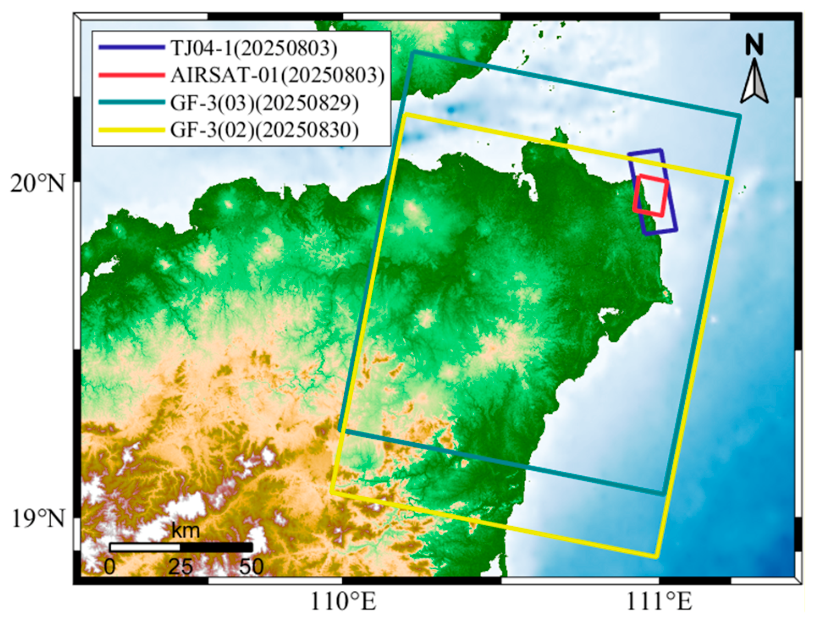
The study area is located in the Wengtian coast, Hainan Island (110.92°E–111.03°E, 19.90°N–20.02°N). Figure 1 shows its geographical location. The red box delineates the area used for bathymetric inversion. Wengtian Town lies in northeastern Wenchang City of Hainan Province. Its coastal waters are situated along the northeastern margin of Hainan Island and in the northwestern South China Sea. The coastline generally extends from northwest to southeast and consists mainly of sandy coast [22]. According to the global wave-period distribution in [17], the Wengtian coast of Hainan Island is dominated by short-period waves. Owing to its geographical setting, this area is influenced year-round by monsoons, tides, and waves. These processes create a complex hydrodynamic environment [23]. In addition, storm surges pose substantial threats to nearshore infrastructure and coastal marine industries [24]. Therefore, timely and accurate bathymetric information of this region is essential for coastal disaster prevention and mitigation, marine engineering, and sustainable coastal-zone management.

2.2. Analysis of the Short-Period Wave Dominance

For the Wengtian coast of Hainan Island, this section analyzes wave period distributions to demonstrate the area’s dominance by short-period waves. The impact of this wave dominance on coastal bathymetric inversion is then quantitatively evaluated, providing the foundation for the proposed method.

2.2.1. Statistical Analysis of Wave Periods

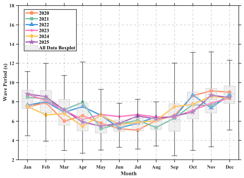
To quantitatively characterize the short-period wave dominance along the Wengtian coast of Hainan Island, peak wave period data from 2020 to 2025 were downloaded from the European Center for Medium-Range Weather Forecasts (ECMWF) ERA5 reanalysis dataset. The statistics are presented in Figure 2. The box plots denote the six-year monthly means, while the curves represent the monthly means of each year.

As shown in Figure 2, wave periods along the Wengtian coast are mainly distributed within the range of 5–9 s, which is significantly lower than the long-period thresholds adopted in previous SAR-based bathymetric inversion studies [4,5,9,12,18,19,20]. This indicates that the area is a typical short-period wave-dominated region. In the distribution of wave periods, those from June to August are even shorter, indicating stronger short-period wave dominance. Therefore, SAR data acquired during these months should be preferentially selected to fully validate the effectiveness of the proposed method under short-period wave conditions.

2.2.2. Impact of Short-Period Wave Dominance on Bathymetric Inversion

This section analyzes the impact of short-period wave dominance on bathymetric inversion. Building on the concept of sensitivity to wavenumber proposed by Holman et al. [25] in the cBathy algorithm, this study extends it to the wave period. The bathymetric sensitivity to wave period variations, denoted $S_T$, is defined as the ratio of the relative change in bathymetry to the relative change in wave period:

$$S_T={\displaystyle \frac{\partial d/d}{\partial T/T}}$$

(1)

where $d$ is the bathymetry and $T$ is the wave period.

To further obtain the analytical expression for this sensitivity, this study introduces the linear dispersion relation given by Equation (2). This relation establishes the connection among wavelength, wave period, and water depth.

$$d={\displaystyle \frac{\lambda }{2\pi }}\mathrm{atanh}\left({\displaystyle \frac{2\pi \lambda }{g{T}^2}}\right)$$

(2)

where $\lambda$ is the wavelength, $\mathrm{atanh}$ is the inverse hyperbolic tangent function, and $g$ is the gravitational acceleration.

Under the condition of a fixed wavelength $\lambda$, substituting Equation (2) into Equation (1) and taking the partial derivative with respect to the wave period $T$. Since the water depth decreases with increasing wave period, $S_T$ is always negative. Taking its absolute value yields the analytical expression for the sensitivity:

$$\left|S_T\right|={\displaystyle \frac{\sinh (2kd)}{kd}}$$

(3)

where $k(=2\pi /\lambda )$ is the wavenumber, which can be obtained by numerically solving the linear dispersion relation for the given wave period and water depth using the Newton iteration method.

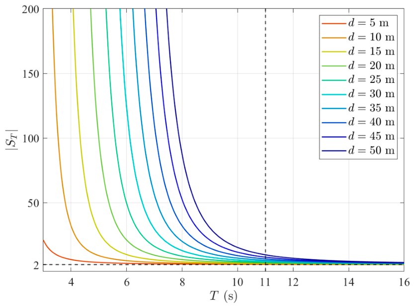
This parameter $\left|S_T\right|$ is dimensionless and represents the factor by which the relative change in wave period is amplified into the relative change in water depth after inversion. It approaches a constant value of $\left|S_T\right|=2$ in the shallow-water limit and diverges exponentially in the deep-water limit. This indicates that the sensitivity to wave period increases markedly with increasing water depth. Figure 3 shows the variation in sensitivity with wave period and water depth, with wave periods ranging from 3 to 16 s and water depths from 5 to 50 m.

As shown in Figure 3, for a fixed wave period, sensitivity $\left|S_T\right|$ increases monotonically with water depth. The increase becomes more dramatic with increasing water depth. For a fixed water depth, the sensitivity $\left|S_T\right|$ decreases monotonically with increasing wave period. When the wave period exceeds 11 s, the curves for all water depths converge toward the shallow-water limit of $\left|S_T\right|=2$. When the wave period is less than 11 s, the slope of the curves increases sharply, and the error is amplified by more than tenfold. This indicates that bathymetric inversion errors from short-period waves are far larger than those from long-period waves, and that the inversion results are highly unstable.

For the wave period range of 5–9 s along the Wengtian coast, $\left|S_T\right|$ is significantly larger, far exceeding the corresponding values for long-period areas. This implies that bathymetric inversion in this area is subject to large errors and poor stability. The above analysis theoretically demonstrates that bathymetric inversion errors in short-period wave-dominated areas are far larger than those in long-period wave-dominated areas. As a typical short-period wave-dominated area, the Wengtian coast poses considerable challenges for bathymetric inversion.

3. Data

3.1. Multi-Temporal SAR Data

The dataset comprises four SAR images acquired over the Wengtian coast of Hainan Island in August 2025. The statistical analysis in Section 2.2.1 indicates that wave periods are relatively short from June to August. The mean wave period in August 2025 was approximately 7 s, making these data suitable for validating the proposed method in short-period wave-dominated areas.

The spatial coverage of the four SAR images is shown in Figure 1. They were acquired by the TJ04-1, AIRSAT-01, GF-3(03), and GF-3(02) satellites. Their acquisition times and key sensor parameters are summarized in

Table 1. The information of the multi-temporal SAR data used in this paper.

No.	Acquisition Time (UTC)	Satellites	Band	Polarization	Pixel Resolution (Azimuth × Range)	Swath (Azimuth × Range)	Wave Period
1	20250803 15:14:18	TJ04-1	X	VV	0.50 m × 0.50 m	26.7 km × 10.5 km	8.08 s
2	20250803 22:54:04	AIRSAT-01	Ku	HH	0.55 m ×0.55 m	13.2 km × 11 km	7.65 s
3	20250829 22:37:17	GF-3(03)	C	HH	4.78 m × 8.64 m	127.3 km × 109.8 km	8.96 s
4	20250830 22:35:06	GF-3(02)	C	HH	4.77 m × 8.66 m	127.4 km × 110.2 km	8.10 s

. Among them, the wave period is calculated using (10). TJ04-1 is an X-band commercial SAR satellite developed and launched by MINOSPACE in February 2022. AIRSAT-01 is a Ku-band commercial SAR satellite developed and launched by AIRSAT Technology Group in September 2024 [26]. GF-3(02) and GF-3(03) are the second and third C-band SAR satellites of the Gaofen-3 series, launched in November 2021 and April 2022, respectively, and both offer strong capabilities for ocean and coastal monitoring [27,28,29].

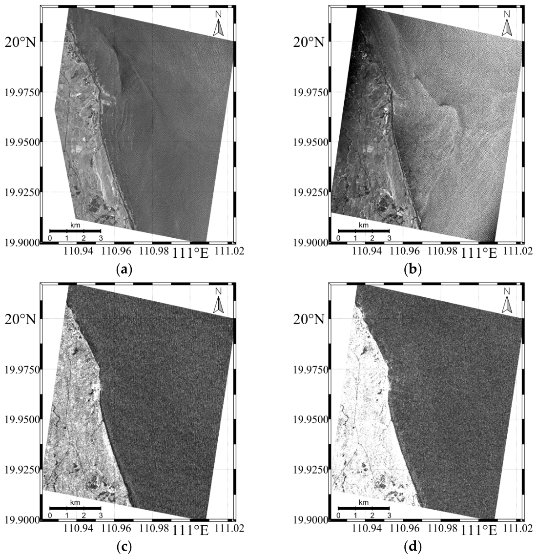
Given the substantial differences in swath width among the four datasets, the AIRSAT-01 coverage was selected as the study area to exploit the advantages of multi-temporal fusion. The other three SAR images were cropped to the same spatial extent. The cropped images are shown in Figure 4 in chronological order of acquisition. Note that part of the land area in Figure 4a is not fully covered, but this does not affect the bathymetric inversion.

As shown in Figure 4, the four SAR images display wave patterns with varying levels of clarity due to their different spatial resolutions. Owing to their higher spatial resolutions, the TJ04-1 (Figure 4a) and AIRSAT-01 (Figure 4b) images show clearer wave patterns but are also affected by other oceanic phenomena. In contrast, the GF-3(03) image (Figure 4c) and the GF-3(02) image (Figure 4d) show blurred wave patterns, primarily due to speckle noise and spatial resolution limitations.

Although these images differ markedly in band, polarization, and spatial resolution, all cover the selected study area and exhibit clearly visible wave patterns. They satisfy the basic requirement for wave-based coastal bathymetric inversion. Next, the cropped multi-temporal SAR images shown in Figure 4 are used to perform bathymetric inversion.

3.2. Reference Bathymetry Data

The reference bathymetry data used in this study are the Global Multi-Resolution Topography (GMRT) data [30]. GMRT compiles multibeam sonar data collected by research institutions worldwide, gridded seafloor depth data, terrestrial elevation data, and international compilation base maps assembled by the GEBCO community. These data are gridded and integrated into a continuously updated global bathymetric synthesis [31]. The GMRT data have a maximum resolution of 100 m and can be accessed and downloaded at https://www.gmrt.org/.

Further examination confirmed that no high-resolution GMRT multibeam bathymetric data or regional high-resolution bathymetric grids contributed by research institutions are available in the Wengtian coast, Hainan Island. Therefore, the GMRT reference bathymetry used in this study is mainly derived from the GEBCO base grid incorporated into the corresponding GMRT version. The grid spacing is 15 arc seconds. At the study area, this corresponds to approximately 437 m in the east–west direction and 463 m in the north–south direction. It should be noted that these values represent the GEBCO grid spacing and do not necessarily reflect the effective spatial resolution of the measured data. GEBCO does not provide a uniform vertical accuracy for the study area. Its reliability varies with source-data type and spatial coverage. Because in situ bathymetric measurements synchronous with the SAR images are unavailable, the vertical accuracy of the reference bathymetry within the study area cannot be quantified at this time.

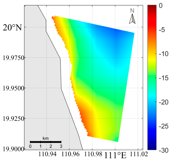
To evaluate the bathymetric inversion results, the downloaded GMRT reference bathymetry was interpolated onto the bathymetric inversion grid for subsequent error calculation. Figure 5 shows the GMRT reference bathymetry along the Wengtian coast of Hainan Island.

3.3. Tidal Data

Variations in the marine environment cause tidal heights to differ over time, leading to differences in the actual inverted water depths. Therefore, tidal correction is required before fusion. In this paper, tidal data from the Baohujiao station provided by the National Marine Data and Information Service were used to correct single-image bathymetric retrievals. The tidal heights at the four SAR acquisition times are listed in

Table 2. Tide heights from Baohujiao Station at the four SAR acquisition times.

No.	SAR Acquisition Time (UTC)	Tidal Height
1	20250803 15:14:18	0.97 m
2	20250803 22:54:04	1.51 m
3	20250829 22:37:17	1.03 m
4	20250830 22:35:06	1.30 m

, with the tidal datum set to 107 cm below mean sea level. Tidal effects are particularly significant in shallow water and must be corrected.

3.4. ECMWF ERA5 Reanalysis Data

The ECMWF ERA5 reanalysis data [32] provide global ocean wave parameters at a temporal resolution of 1 h and a spatial resolution of 0.5° × 0.5°, including the wave period, total significant wave height, swell significant wave height, and wind–sea significant wave height. In this paper, the dataset is used to analyze the recent distribution of wave period over the Wengtian coast. The wave parameters at the SAR acquisition times are also used to compute the Ursell number and wave steepness, which together characterize the nonlinearity of ocean waves. In addition, the swell and wind–sea significant wave heights serve as a quantitative measure of the relative dominance of swell in the prevailing sea state. Therefore, they are adopted as key indicators in the subsequent fusion.

4. Method

The analysis in Section 2.2.2 shows that SAR bathymetric inversion in short-period wave-dominated areas typically faces the challenges of low accuracy and poor stability. From the perspective of the inversion workflow, this challenge arises at two levels: at the wavelength estimation level, uncertainty arises from a single-angle window; at the bathymetric inversion level, results across multiple images differ significantly, and existing fusion methods do not account for quality differences.

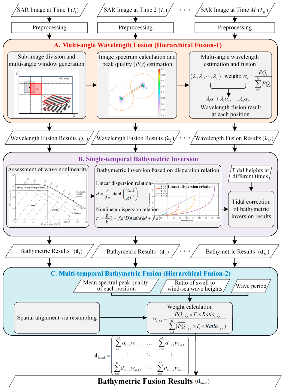
To address the problems at the two levels above, a hierarchical fusion method is developed for SAR-based coastal bathymetric inversion. It introduces adaptive weighted fusion at both the wavelength estimation and bathymetric inversion levels. Figure 6 shows the overall workflow of the method. It mainly consists of three steps: multi-angle wavelength fusion, single-temporal bathymetric inversion, and multi-temporal bathymetric fusion. The first and third steps correspond to the first and second stages of the hierarchical fusion, respectively, while the second step connects the two. The proposed method is described in detail below.

4.1. Multi-Angle Wavelength Fusion

Firstly, the multi-temporal SAR data are preprocessed through radiometric calibration and geocoding. The overlapping area is selected for subsequent processing. Subsequently, multi-angle wavelength estimation and fusion are performed for each SAR image.

4.1.1. Sub-Image Division and Multi-Angle Window Generation

The SAR images at different times are denoted by $I_t$, where $t=1,2,\dots ,M$, and $M$ denotes the number of SAR images. Each SAR image is divided into multiple uniform and overlapping sub-images using a sliding window. In short-period wave-dominated areas, wave patterns appear relatively blurred, and estimating the wavelength from a single-angle window involves considerable uncertainty. To address this, multi-angle windows are generated at each sub-image position [33]. By fully exploiting wave information from windows at different angles at the same position, the reliability of wavelength estimation in a single image can be improved. As a core input parameter for bathymetric inversion, the reliability of the wavelength is essential to the robustness of the proposed method in short-period wave-dominated areas.

Next, estimation is performed on the multi-angle windows at each sub-image position within each image.

4.1.2. Image Spectrum Calculation and Peak Quality Estimation

The two-dimensional Fast Fourier Transform (2D-FFT) is applied to each sub-image to obtain its image spectrum. Ideally, an ocean-wave signal should manifest as a pair of symmetric peaks with highly concentrated energy in the image spectrum. In practice, the peak is broadened by nonlinear wave propagation and speckle noise inherent in SAR imaging, reducing its sharpness. To quantitatively characterize the sharpness of the spectral peak, the peak quality ($PQ$) is defined based on the energy distribution of the image spectrum. The spectral peak quality $P{Q}_s$ corresponding to the $s$-th window is calculated using Equation (4), thereby yielding the spectral peak quality sequence $\left(P{Q}_1,\dots ,P{Q}_N\right)$ for the multi-angle windows at that position.

$$P{Q}_s={\displaystyle \frac{E_{r/10}^s}{E_r^s}}$$

(4)

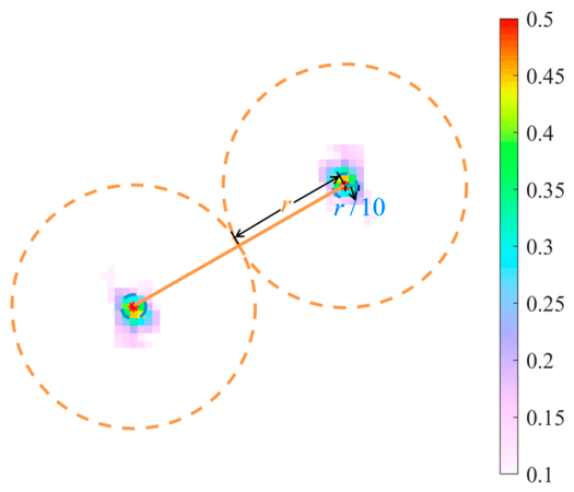
where $E_{r/10}^s$ is the average energy within the circle of radius $r/10$ in the image spectrum of the $s$-th window, $E_r^s$ is the average energy within the circle of radius $r$ in the image spectrum of the $s$-th window, and $r$ is half the distance between the two symmetric spectral peaks.

A schematic illustration of the spectral peak quality calculation is shown in Figure 7. By quantifying the sharpness of the spectral peak, $PQ$ effectively characterizes both the clarity and dominance of the swell component. A higher peak quality indicates more concentrated energy at the peak location, which facilitates more accurate wavelength estimation and, in turn, more reliable bathymetric inversion.

4.1.3. Multi-Angle Wavelength Estimation and Fusion

Firstly, the spectral peak positions are identified from the image spectra computed for the multi-angle windows. The respective swell wavelength ${\lambda }_s$ is calculated using Equation (5), yielding the wavelength sequence $\left({\lambda }_1,\dots ,{\lambda }_N\right)$ for the multi-angle windows.

$${\lambda }_s={\displaystyle \frac{2\pi }{\sqrt{{(k_{px}^s)}^2+{(k_{py}^s)}^2}}}$$

(5)

where ${\lambda }_s$ is the wavelength of the $s$-th window, $k_{px}^s$ and $k_{py}^s$ are the coordinates of the spectral peak position in the image spectrum of the $s$-th window.

Next, the normalized spectral peak quality ${\alpha }_s$ is used as the weight to characterize the differences among multi-angle windows at the same position:

$${\alpha }_s={\displaystyle \frac{P{Q}_s}{{\displaystyle \sum _{s=1}^{n}P{Q}_s}}}$$

(6)

where ${\alpha }_s$ is the normalized weight of the wavelength estimate from the $s$-th window.

Finally, the wavelengths are fused based on the corresponding weights of each multi-angle window at the same position, and the fused wavelength ${\lambda }_{\mathrm{fused}}$ at that position is calculated, completing the first part of the hierarchical fusion.

$${\lambda }_{\mathrm{fused}}={\displaystyle \sum _{s=1}^N{\lambda }_s}{\alpha }_s$$

(7)

The above process is repeated for other positions and temporal SAR data, yielding the wavelength fusion field ${\mathsf{\lambda }}_t$ for each SAR image, which serves as input to the subsequent coastal bathymetric inversion.

4.2. Single-Temporal Bathymetric Inversion

Before performing bathymetric inversion based on the wavelength fusion results from Section 4.1, the degree of wave nonlinearity must first be assessed to select the applicable dispersion relation for coastal bathymetric inversion. Since tidal height varies over time, the single-temporal bathymetric inversion results need to be corrected using the tidal data provided in Section 3.3.

4.2.1. Assessment of Wave Nonlinearity

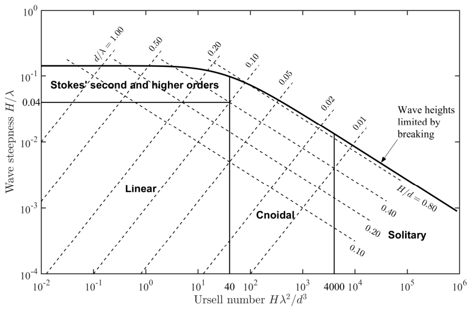
The propagation of ocean waves is often accompanied by enhanced nonlinear effects, rendering linear wave theory inapplicable. Therefore, before performing bathymetric inversion, the wave nonlinearity needs to be assessed to determine whether the sea state at the corresponding time satisfies the linear or nonlinear wave theory. Based on theoretical derivation and experimental measurements, Hedges [34] characterized the validity ranges of different wave theories using two parameters—namely, the Ursell number ($Ur$) and the wave steepness ($WS$)—as shown in Figure 8. The Ursell number combines the relative magnitudes of wave height, wavelength, and water depth, and quantifies the degree of nonlinearity introduced by shallow-water effects [35]. Wave steepness is the ratio of wave height to wavelength. The greater the steepness, the more the wave profile deviates from a sinusoidal shape [15]. The two parameters are defined as follows:

$$Ur={\displaystyle \frac{H·{\lambda }^2}{d^3}}$$

(8)

$$WS={\displaystyle \frac{H}{\lambda }}$$

(9)

where $H$ is the wave height, $\lambda$ is the wavelength, and $d$ is the water depth.

The Ursell number and wave steepness are computed at each SAR acquisition time. The resulting values are compared with the validity criteria of the linear wave theory to determine whether the wave field falls within the linear regime. If the Ursell number is less than 40 and the wave steepness is less than 0.04, the linear wave theory is satisfied, and the linear dispersion relation is selected for bathymetric inversion. Otherwise, the nonlinear dispersion relation is selected for bathymetric inversion.

4.2.2. Bathymetric Inversion Based on Dispersion Relation

If the linear wave theory is satisfied, the linear dispersion relation given by Equation (2) is used directly to invert for water depth, with the fused wavelength and the estimated wave period as inputs. Owing to the complexity of the marine environment, it is generally difficult to measure the wave period at the time of SAR acquisition, and even more so for individual sub-images in shallow waters. In practice, an initial estimate of the wave period is obtained from the linear dispersion relation for deep water, as given in Equation (10), which provides its lower value. This final value is then adjusted iteratively based on the inverted depths to obtain the final wave period.

$$T_{\mathrm{deep}}=\sqrt{{\displaystyle \frac{2\pi {\lambda }_{\mathrm{deep}}}{g}}}$$

(10)

where $T_{\mathrm{deep}}$ is the deep-water wave period and ${\lambda }_{\mathrm{deep}}$ is the wavelength estimated from a deep-water sub-image.

When the linear wave theory is not applicable, a nonlinear dispersion relation must be used for bathymetric inversion. Catalán and Haller [36] compared several nonlinear models and found that the composite model proposed by Kirby and Dalrymple [37] performs best. Equation (11) gives the corresponding nonlinear dispersion relation. This relation asymptotically approaches the third-order Stokes theory in deep water and the Hedges theory in shallow water. This maintains good accuracy over a wide range of relative water depths. The water depth at each location is then retrieved by solving this dispersion relation.

$$c^2={\displaystyle \frac{g}{k}}(1+f_1{\epsilon }^{2}D)\tanh (kd+f_2\epsilon )$$

(11)

where $c$ (=$\lambda /T$) is the phase speed, $k$ (=$2\pi /\lambda$) is the magnitude of the wavenumber vector $k$, $\epsilon =kA=kH/2$, $A$ (=$H/2$) is the wave amplitude, and $H$ is the wave height. The expressions for $D$, $f_1$ and $f_2$ are given by

$$D={\displaystyle \frac{8+\cosh (4kd)-2{\tanh }^2(kd)}{8{\sinh }^4(kd)}}$$

(12)

$$f_1(kd){=\tanh }^5(kd),f_2(kd)={\left({\displaystyle \frac{kd}{\sinh (kd)}}\right)}^4$$

(13)

4.2.3. Tidal Correction of Bathymetric Inversion Results

After coastal bathymetric inversion is performed based on the dispersion relation, the bathymetric inversion result $d_t^{\mathrm{dispersion}}$ for each SAR image is obtained. It then needs tidal correction to obtain the actual water depth $d_t^{\mathrm{corrected}}$:

$$d_t^{\mathrm{corrected}}=d_t^{\mathrm{dispersion}}-h_t^{\mathrm{tide}}+{\Delta }_{\mathrm{datum}}$$

(14)

where $d_t^{\mathrm{corrected}}$ is the bathymetric inversion result for time $t$ after tidal correction, $d_t^{\mathrm{dispersion}}$ is the bathymetric inversion result for time $t$ solved from the dispersion relation, $h_t^{\mathrm{tide}}$ is the tidal height for time $t$, and ${\Delta }_{\mathrm{datum}}$ is the difference between the mean sea level and the tidal datum.

4.3. Multi-Temporal Bathymetric Fusion

Since the multi-temporal SAR data have different spatial resolutions, direct coastal bathymetric fusion is not feasible. Spatial alignment is therefore required at either the SAR data level or the bathymetric inversion result level. Due to speckle noise, directly unifying the spatial resolution of multi-temporal SAR data by interpolation would inevitably introduce additional errors. Therefore, this study resamples the single-temporal bathymetric inversion results to enable spatial alignment for bathymetric fusion. To prevent the detailed information of the bathymetric inversion results from being lost, the bathymetric inversion result with the highest spatial resolution is used as the reference, and the other inversion results are resampled accordingly.

The imaging quality and sea conditions of SAR images at different times differ significantly. Such differences cause the single-temporal bathymetric inversion results to vary in accuracy and stability. In this case, simple mean fusion or Kalman filter fusion is insufficient to suppress the influence of low-quality inversion results. To address this, this study adopts adaptive weighted fusion to achieve more robust bathymetric fusion.

For the adaptive weighted fusion, this study comprehensively considers parameters such as spectral peak quality, wave period, and the ratio of swell to wind–sea significant wave heights. Firstly, higher spectral peak quality corresponds to sharper spectral peaks [10], leading to more reliable wavelength estimation and more trustworthy bathymetric inversion results. In this paper, the spectral peak quality at each position in each SAR image is characterized as the mean of the spectral peak quality values across the multi-angle windows at that position. Secondly, the wave period significantly affects the accuracy of bathymetric inversion. By comparison, bathymetric inversion errors are lower under long-period wave conditions, while they are significantly higher under short-period wave conditions [4,10,16]. Finally, the ratio of swell to wind–sea significant wave heights reflects the degree of swell dominance. Swell dominance is an important factor affecting the accuracy of bathymetric inversion [12], since the swell component is generally more reliable than the wind–sea component [38]. In this paper, the ratio is calculated from the swell wave height and the wind–sea wave height, both downloaded from the ECMWF website. A larger ratio indicates a more dominant swell, which better satisfies the ideal sea state assumption of SAR-based bathymetric inversion and is more favorable for coastal bathymetric inversion.

Next, the normalized weights are calculated using Equation (15) based on the spectral peak quality, the wave period, and the ratio of swell to wind–sea significant wave heights. A multiplicative form is adopted to jointly characterize the reliability of each inversion result. A high weight is assigned only when all three parameters are relatively large. In contrast, a low value of any parameter reduces the contribution of the corresponding result to the fusion process.

$$w_{i,j,t}={\displaystyle \frac{{\overline{PQ}}_{i,j,t}\times T_t\times Rati{o}_{i,j,t}}{{\displaystyle \sum _{t=1}^M({\overline{PQ}}_{i,j,t}\times T_t\times Rati{o}_{i,j,t})}}}$$

(15)

where $i,j$ is the sub-image at the $i$-th row and $j$-th column, $t$ is the $t$-th SAR image, $M$ is the total number of SAR images, $\overline{PQ}$ is the mean peak quality across the multi-angle windows at the same location, and $T_t$ is the estimated wave period of the $t$-th SAR image. $Rati{o}_{i,j,t}$($=H_{i,j,t}^{\mathrm{swell}}/H_{i,j,t}^{\mathrm{wind}\mathrm{sea}}$) is the ratio of swell to wind–sea significant wave heights, and $H^{swell}$ and $H^{windsea}$ are the swell and wind–sea significant wave heights, respectively.

Furthermore, because each product is normalized by the sum of the products across all SAR images, the final weights depend on the relative variation in the three parameters among the images rather than on their absolute magnitudes. For example, dividing the values of one parameter by its maximum across all SAR images is equivalent to dividing both the numerator and denominator of Equation (15) by the same constant. This operation is therefore mathematically equivalent to the original formulation and does not change the final weights.

Based on the single-temporal bathymetric inversion results and their corresponding weights, the results are fused to obtain $d_{\mathrm{fused}}$ based on Equation (16). The proposed method adaptively adjusts the inversion weights at different positions within each SAR image based on the actual sea conditions, thereby ensuring more reliable bathymetric estimates.

$$d_{\mathrm{fused}}=\left(\begin{array}{ccc}{\displaystyle \sum _{t=1}^M{d}_{1,1,t}}{w}_{1,1,t}& \dots & {\displaystyle \sum _{t=1}^M{d}_{1,n,t}}{w}_{1,n,t}\\ ⋮& \ddots & ⋮\\ {\displaystyle \sum _{t=1}^M{d}_{m,1,t}}{w}_{m,1,t}& \dots & {\displaystyle \sum _{t=1}^M{d}_{m,n,t}}{w}_{m,n,t}\end{array}\right)$$

(16)

where $m$ and $n$ are the number of rows and the number of columns of the resampled bathymetric results, respectively.

5. Results

To demonstrate the effectiveness of the proposed method in short-period wave-dominated areas, experimental validation is conducted using the Wengtian coast on Hainan Island as a case study.

5.1. Multi-Angle Wavelength Fusion Results

5.1.1. Peak Quality Calculation Results

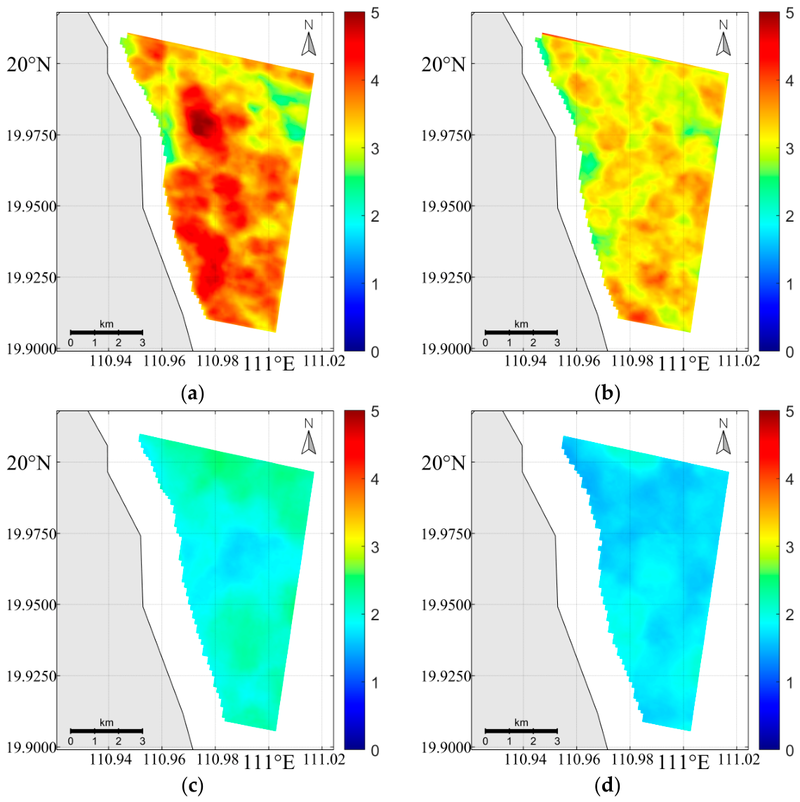
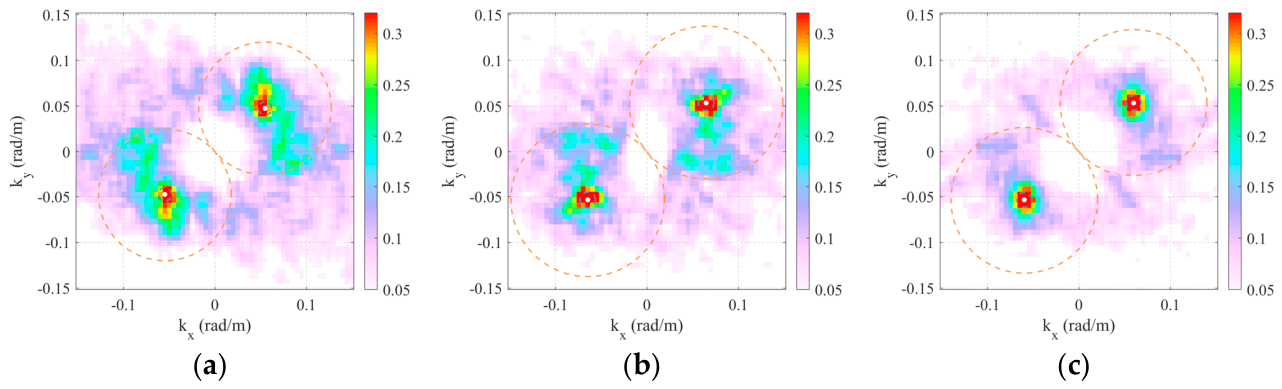
Firstly, each SAR image is divided into sub-images, and the corresponding image spectrum is calculated. To eliminate the influence of the zero-frequency component on peak identification, a low-pass filter is applied to the image spectrum; the spectral peak is then located in the filtered spectrum, and its quality is calculated using Equation (4). Examples of image spectra with different $PQ$ values are shown in Figure 9. The $PQ$ value reflects how concentrated the spectral energy is at the peak: the higher the $PQ$, the more concentrated the energy is around the peak, and the more pronounced the suppression of energy in other regions of the wavenumber domain.

Next, multi-angle windows are generated at each position, and the corresponding spectral peak quality $\left(P{Q}_1,\dots ,P{Q}_N\right)$ and wavelength $\left({\lambda }_1,\dots ,{\lambda }_N\right)$ are calculated. The mean multi-angle spectral peak quality results for the four SAR images are shown in Figure 10.

As shown in Figure 10, the TJ04-1 and AIRSAT-01 images yield overall higher $PQ$ values than the two GF-3 images, mainly because of their finer spatial resolutions. In addition, the four SAR images are affected by land–sea contamination over different regions. After interpolation, the $PQ$ maps of the GF-3(03) and GF-3(02) images are more strongly affected by such contamination near the coast due to their lower spatial resolutions.

5.1.2. Wavelength Fusion Results

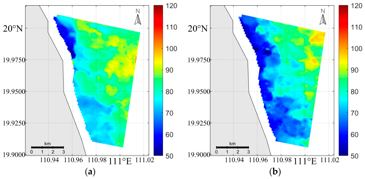
For each sub-image, multi-angle windows are generated to compute the corresponding sequence of peak quality $\left(P{Q}_1,\dots ,P{Q}_N\right)$ and wavelength estimates $\left({\lambda }_1,\dots ,{\lambda }_N\right)$. The multi-angle wavelength estimates at each position are then fused using Equation (7). Repeating this for the four SAR images yields the fused wavelength results shown in Figure 11.

As shown in Figure 11, the GF-3(03) image yields the longest wavelengths and correspondingly the largest wave period, which is favorable for bathymetric inversion at a given water depth. In contrast, the wavelengths of the other three SAR images fall within a similar range. The fused wavelengths are then used as inputs for the subsequent bathymetric inversion.

5.2. Single-Temporal Bathymetric Inversion Results

5.2.1. Wave Nonlinearity Calculation Results

Before performing bathymetric inversion, the degree of wave nonlinearity is assessed to select an appropriate dispersion relation. The Ursell number and the wave steepness jointly determine wave nonlinearity. The ERA5 reanalysis data at the location (110.98°E, 19.95°N) within the study area are selected to calculate the Ursell number and the wave steepness. The corresponding results are given in

Table 3. Ursell number and wave steepness computed from the ECMWF ERA5 reanalysis data.

No.	SAR Acquisition Time (UTC)	ECMWF ERA5 Time (UTC)	Ursell Number	Wave Steepness
1	20250803 15:14:18	20250803 15:00:00	1.7184	0.0123
2	20250803 22:54:04	20250803 23:00:00	1.4576	0.0162
3	20250829 22:37:17	20250829 23:00:00	6.0947	0.0229
4	20250830 22:35:06	20250830 23:00:00	2.2664	0.0130

. Although ERA5 reanalysis data differ somewhat from the SAR imaging times, the gaps are all within 30 min, indicating a high degree of spatiotemporal matching.

According to the values listed in Table 3 and the validity ranges shown in Figure 8, the wave fields associated with all four SAR images fall inside the validity range of the linear wave theory. The linear dispersion relation in Equation (2) is therefore used for the coastal bathymetric inversion.

5.2.2. Bathymetric Inversion Results After Tidal Correction

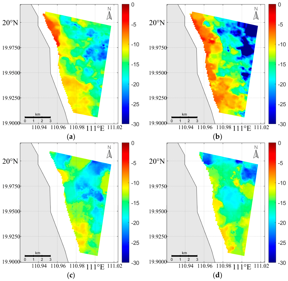
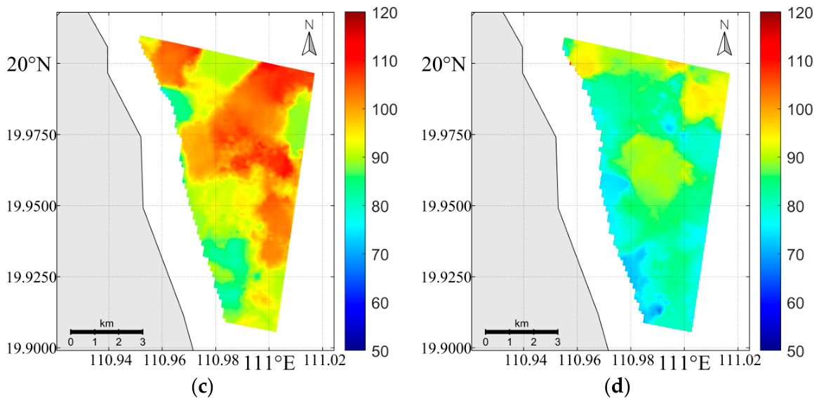
The wave periods estimated from the four SAR images are 8.08 s, 7.65 s, 8.96 s, and 8.10 s, respectively. Comparison with the ERA5 peak wave periods at the corresponding SAR acquisition times yielded a Pearson correlation coefficient of 0.98 and an RMSE of 1.56 s. This indicates highly consistent temporal variations despite some differences in magnitude. The SAR-derived and ERA5 peak wave periods are not fully equivalent because they differ in wave-component representation, spatial scale, and calculation method. Since the SAR-derived periods are more closely related to the wave components visible in the SAR images, each SAR-derived period was adopted as the representative wave period for the corresponding full SAR images. Combining these wave periods with the fused wavelengths shown in Figure 11, the linear dispersion relation is then applied to invert the coastal bathymetry. The resulting depths are corrected for tidal effects using the data from the Baohujiao tide gauge station, provided by the National Marine Data and Information Service. The tidally corrected bathymetric results, with a 100 m spatial resolution, are shown in Figure 12.

Notable discrepancies are observed among the bathymetric retrievals derived from the four SAR images, suggesting that single-image inversion is relatively unstable. Although all four images yield valid retrievals, the TJ04-1 and AIRSAT-01 images preserve finer bathymetric details. The TJ04-1 and AIRSAT-01 SAR images show relatively consistent trends in water depth below 15 m. Because the AIRSAT-01 SAR image has a smaller wave period, its bathymetric inversion results exhibit a larger fluctuation range. In its deeper regions, the corresponding dispersion relation has a steeper slope, thereby producing larger bathymetric inversion errors. The GF-3(03) and GF-3(02) images mainly reflect the overall bathymetric trends rather than fine-scale local features. Their results are affected by land interference over a larger area, providing almost no inversion information for water depths below 10 m.

5.2.3. Bathymetric Inversion Error Assessment Results

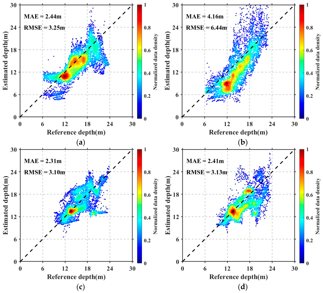
To quantitatively assess discrepancies between single-temporal bathymetric retrievals and the reference bathymetry, the four sets of retrievals are compared with the reference at their corresponding locations, and the resulting error scatter plots are shown in Figure 13. The mean absolute error (MAE) and root mean square error (RMSE) are computed using

$$\mathrm{MAE}={\displaystyle \frac{1}{\mathcal{N}}}{\displaystyle \sum _{\mathcal{l}=1}^{\mathcal{N}}\left|d_{\mathrm{derived}}^{\mathcal{l}}-d_{\mathrm{reference}}^{\mathcal{l}}\right|}$$

(17)

$$\mathrm{RMSE}=\sqrt{{\displaystyle \frac{1}{\mathcal{N}}}{\displaystyle \sum _{\mathcal{l}=1}^{\mathcal{N}}{\left(d_{\mathrm{derived}}^{\mathcal{l}}-d_{\mathrm{reference}}^{\mathcal{l}}\right)}^2}}$$

(18)

where $d_{\mathrm{reference}}^{\mathcal{l}}$ and $d_{\mathrm{derived}}^{\mathcal{l}}$ are the reference bathymetry and derived bathymetry of the $\mathcal{l}$-th sub-image in the study area, and $\mathcal{N}$ represents the number of sub-images.

As shown in Figure 13, the bathymetric inversion errors of the GF-3 (03) and GF-3 (02) SAR images in the study area differ only slightly, and both can hardly invert water depth accurately below 10 m. Limited by their spatial resolution, their bathymetric inversion results mainly reflect the trend of water depth variation in this area. Among them, the GF-3 (03) SAR image has the lowest bathymetric inversion error, and its overall water depth variation trend is highly consistent with the reference bathymetry. Because the reference bathymetry contains relatively few details, the TJ04-1 and AIRSAT-01 SAR images, which have higher spatial resolution, show larger bathymetric inversion errors. However, they provide a wider bathymetric inversion range and are affected by land interference over a smaller area. Since the AIRSAT-01 SAR image was acquired at the smallest wave period, the error in bathymetric inversion based on the linear dispersion relation is larger.

It should be noted that the errors calculated in this paper reflect the combined effects of SAR-based bathymetric inversion errors, uncertainty in the GMRT reference data and potential changes in the actual seabed morphology. The GMRT bathymetry is compiled from multiple data sources. The observation dates of these source data do not coincide with the SAR acquisition times. Consequently, the GMRT bathymetry may not accurately represent the actual seabed state at those times. If the seabed morphology changed over the time covered by the different SAR acquisitions, these actual changes would also contribute to the differences between the SAR-derived bathymetry and the GMRT reference bathymetry. Because no in situ bathymetric measurements synchronous with each SAR image are currently available, the contributions from inversion errors, reference-data uncertainty and actual seabed changes cannot be quantified separately. Therefore, the calculated errors should be interpreted as the overall discrepancies between the SAR-derived bathymetry and the GMRT reference bathymetry. This is one of the main limitations of the present case study.

5.3. Multi-Temporal Bathymetric Fusion Results

First, the bathymetric inversion result of the AIRSAT-01 SAR data is used as the reference to resample other temporal bathymetric inversion results and mean peak quality results. On this basis, the differences in the mean peak quality, wave period, and the ratio of swell to wind–sea wave heights among the four SAR images are compared, as shown in

Table 4. Comparison of the mean peak quality, wave period, and ratio of swell to wind–sea significant wave heights among the four SAR images.

No.	SAR Acquisition Time (UTC)	Mean Peak Quality	Wave Period (s)	Ratio of Swell to Wind–Sea Wave Heights
1	20250803 15:14:18	3.53	8.08	1.66
2	20250803 22:54:04	3.13	7.65	1.82
3	20250829 22:37:17	2.08	8.96	0.72
4	20250830 22:35:06	1.80	8.10	2.16

.

Based on the combined analysis of mean peak quality, wave period, and ratio of swell to wind–sea wave heights in Table 4, the TJ04-1 SAR image achieves the highest spectral peak quality. The AIRSAT-01 SAR image has a slightly lower spectral peak quality than TJ04-1 but exhibits a higher ratio of swell to wind–sea wave heights. The GF-3 (03) SAR image has lower spectral peak quality but longer wavelengths and larger wave periods, favoring water depth inversion. The GF-3 (02) SAR image also has lower spectral peak quality but has the highest ratio of swell to wind–sea wave heights, reaching up to twice that of the others. These results show that the four SAR images perform differently across the various parameters, yet each exhibits favorable performance in one or two of them. Therefore, the four images can complement one another to achieve high-accuracy bathymetric fusion.

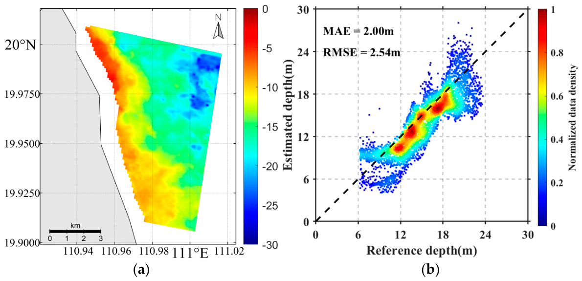
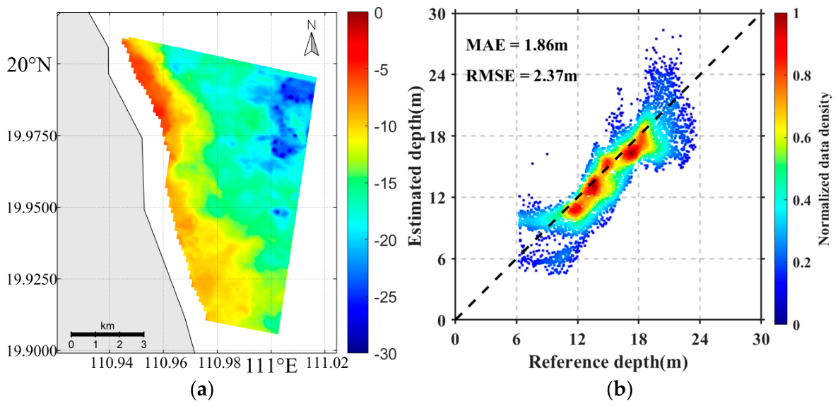
Next, the single-temporal bathymetric inversion results are fused based on spectral peak quality, wave period, and ratio of swell to wind–sea wave heights for each SAR image. The results are shown in Figure 14a. Compared with the reference bathymetry shown in Figure 5, the bathymetric inversion result from the proposed method is fairly consistent with it, with water depths ranging from 0 to 30 m. Compared with the reference seabed topography, the bathymetric fusion result of the proposed method can reveal more detailed information.

An error scatter plot between the fused bathymetry and the reference bathymetry was generated, along with calculations of the MAE and RMSE, as shown in Figure 14b. As shown, the points in the error scatter plot between the bathymetric fusion result and the reference bathymetry are relatively concentrated. Compared with the best single-temporal inversion results, the bathymetry inversion error is still significantly reduced. The MAE decreases from 2.31 m to 1.86 m, a reduction of 19.5%, and the RMSE decreases from 3.10 m to 2.37 m, a reduction of 23.5%, fully demonstrating the advantage of hierarchical fusion.

In summary, this study demonstrates underwater topography detection using four SAR images acquired over the Wengtian coast of Hainan Island in August 2025. Compared with single-temporal bathymetric inversion results, the proposed method shows better agreement with the reference bathymetry. The remaining discrepancies are mainly attributable to actual changes in the underwater topography and to the non-negligible uncertainties inherent in the reference bathymetry. Future work will combine temporally coincident in situ bathymetric measurements with a denser time series of SAR images to further assess the effects of seabed changes on multi-temporal fusion results.

6. Discussion

First, the differences between linear and nonlinear dispersion relations in bathymetric inversion are compared to evaluate the rationale for selecting a dispersion relation based on wave nonlinearity. In addition, the applicability of the proposed method to short-period wave-dominated areas is compared with that of other multi-temporal bathymetric fusion methods such as mean fusion and Kalman filter fusion. Finally, the sensitivity analysis of fusion weights is discussed to assess the stability of the proposed weighting scheme.

6.1. Effect of Dispersion Relation Selection

In Section 5.2.1, the calculation results of the Ursell number and the wave steepness indicate that the study area satisfies the linear wave theory, so the linear dispersion relation is selected to invert the single-temporal bathymetry. To further compare the effects of the linear and nonlinear dispersion relations on the proposed method, this study performs bathymetric inversion on the same dataset using the nonlinear dispersion relation (the Kirby–Dalrymple composite model [37]) given in Equation (11), with the results shown in Figure 15.

Comparing the bathymetric inversion results in Figure 14a and Figure 15a, the bathymetry inverted using different dispersion relations shows little difference. However, comparing the error scatter plots in Figure 14b and Figure 15b, the bathymetric error from the nonlinear dispersion relation is still larger than that from the linear one. This effectively confirms the validity of the applicable ranges of different wave theories summarized by Hedges [34]. Although wave nonlinearity gradually strengthens during wave propagation, the linear dispersion relation remains accurate under conditions that satisfy the linear wave theory. In such cases, it achieves accuracy comparable to, or even better than, the nonlinear method and is computationally simpler. The Kirby–Dalrymple nonlinear dispersion relation has broader theoretical applicability, but its higher-order correction terms can bias inversion results when the sea state is well described by linear theory. By contrast, the linear dispersion relation provides more stable parameter estimation and higher inversion accuracy under such conditions. These results further verify the reasonableness of the adaptive dispersion relation selection strategy proposed in this paper.

6.2. Effect of Different Fusion Methods

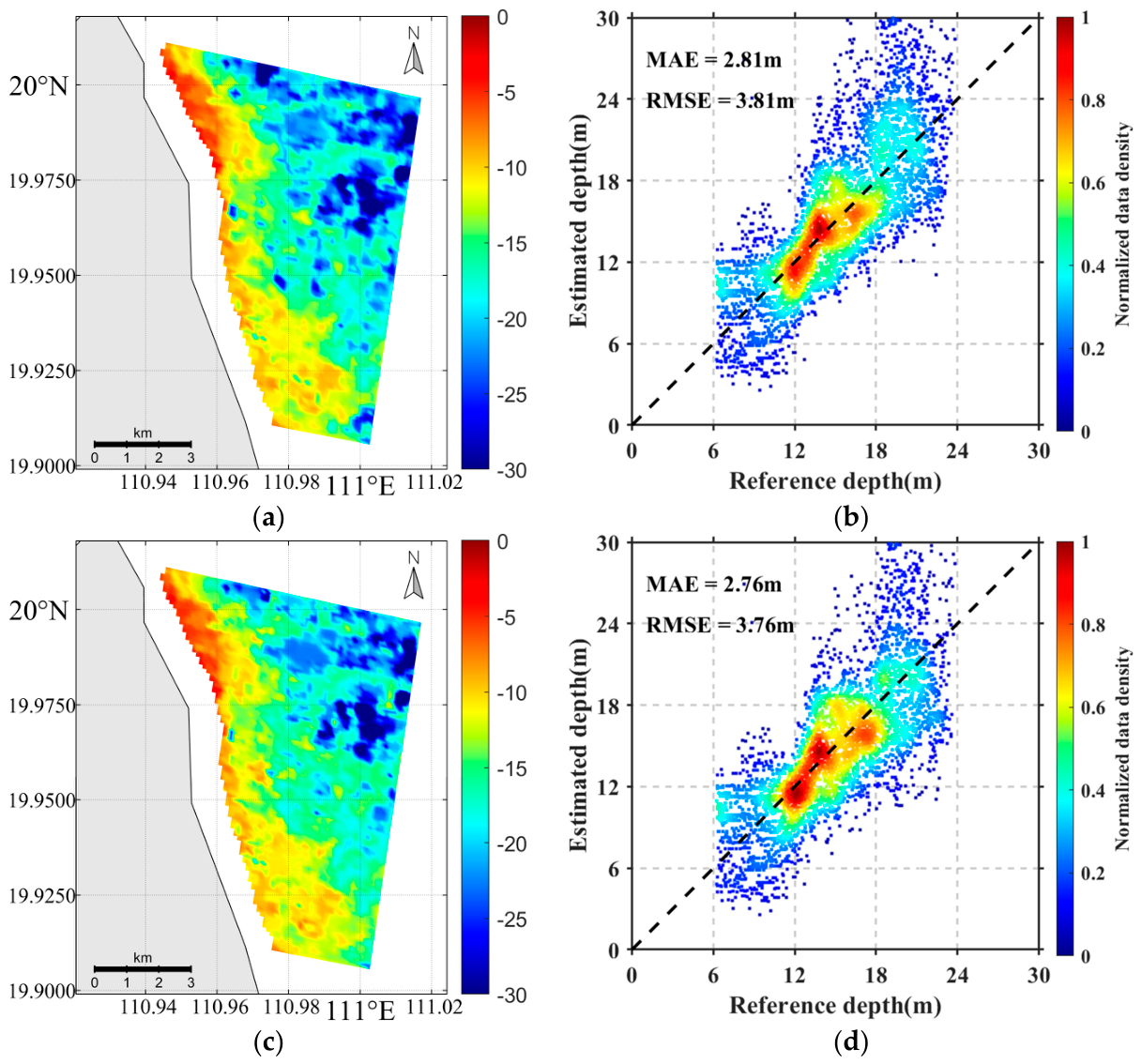
In multi-temporal coastal bathymetric fusion, this study fully considers the influence of peak quality, wave period, and ratio of swell to wind–sea wave heights, with weights varying across different positions within the same image. To further demonstrate the effectiveness of the proposed fusion method, this study compares it with the existing mean fusion method [10] and the Kalman filter fusion method [9] on the same dataset. The Kalman filter was implemented following [9] using a time-invariant parameter model. Specifically, the state transition matrix, observation matrix, process noise covariance matrix, and observation noise covariance matrix remained constant across acquisition times. The bathymetric inversion results and their error scatter plots are shown in Figure 16.

As shown in Figure 16, the mean fusion result in Figure 16a is independent of the image order and assigns equal weights to the bathymetric retrieval results of the four SAR images. Since these results differ considerably among the four images, this fusion method performs poorly in the study area. In Figure 16c, the single-temporal bathymetric retrieval results are provided to the Kalman filter fusion in chronological order of SAR imaging time. It should be noted that this study includes only four SAR acquisitions. This limited number makes it difficult to evaluate the Kalman filter’s convergence performance comprehensively. Therefore, the Kalman filter is used only as a benchmark under the current data and fixed parameter settings. Its results do not represent its general performance with long time series. Owing to the large discrepancies among the four retrieval results and the limited number of images, the fused bathymetry is not sufficiently stable. Since the single-temporal bathymetric inversion errors are large in short-period wave-dominated areas, the points in the error scatter plots of both the mean fusion method (Figure 16b) and the Kalman filter fusion method (Figure 16d) are less concentrated than those of the proposed method. By contrast, the fusion result of the proposed method in Figure 14a is closer to the reference bathymetry. By hierarchically combining wavelength and water depth, errors can be reduced at multiple stages, resulting in good performance in short-period wave-dominated areas.

Table 5. Bathymetric retrieval errors of the mean fusion method, the Kalman filter fusion method, and the proposed method.

Statistics	Mean Fusion Method	Kalman Filter Fusion Method	Proposed Fusion Method
MAE (m)	2.81	2.76	1.86
RMSE (m)	3.81	3.76	2.37

further compares bathymetric inversion errors for the mean fusion method, the Kalman filter fusion method, and the proposed hierarchical fusion method in the coastal area of Wengtian, Hainan Island.

According to the comparison results in Table 5, the mean and Kalman filter fusion methods yield similar bathymetric inversion errors when fusing the four SAR images, and neither outperforms the best single-temporal result. This clearly indicates that, in short-period wave-dominated areas, simple averaging and time-sequential recursive fusion strategies can hardly effectively suppress single-temporal errors. By contrast, the proposed method employs hierarchical fusion of wavelength and water depth with adaptive weights that account for both imaging quality and sea-state conditions, thereby effectively reducing bathymetric retrieval errors.

6.3. Sensitivity Analysis of Fusion Weights

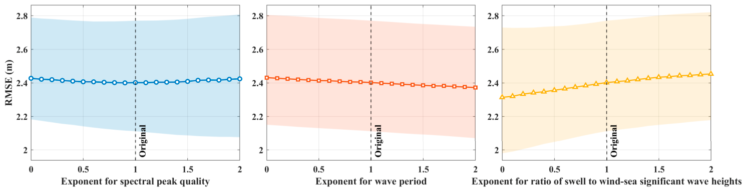
This section presents a sensitivity analysis of the fusion weights defined in Equation (15). The weight is calculated as the product of the spectral peak quality, wave period, and the ratio of swell to wind–sea significant wave heights, and is then normalized by the sum of these products across all SAR images. Increasing or decreasing all values of any one parameter by 20% is mathematically equivalent to multiplying both the numerator and denominator of Equation (15) by the same constant. Therefore, such a change does not alter the relative weights assigned to the bathymetric inversion results from the individual SAR images.

To address this issue, weighting exponents are introduced, and the corresponding weights are calculated using Equation (19). The exponents of the three parameters control their relative differences among the SAR images, thereby enabling an evaluation of the sensitivity of the fused results to each parameter. An exponent of 0 indicates that the corresponding parameter is excluded, whereas setting all three exponents to 1 reproduces the weighting scheme adopted in the proposed method. An exponent greater than 1 enhances the relative influence of the corresponding parameter, while an exponent between 0 and 1 reduces its relative influence.

$$w_{i,j,t}(a,b,c)={\displaystyle \frac{{\overline{PQ}}_{i,j,t}^a\times T_t^b\times Rati{o}_{i,j,t}^c}{{\displaystyle \sum _{t=1}^M\left({\overline{PQ}}_{i,j,t}^a\times T_t^b\times Rati{o}_{i,j,t}^c\right)}}}$$

(19)

where $a$ is the weighting exponent associated with the spectral peak quality, $b$ is the weighting exponent associated with the wave period, and $c$ is the weighting exponent associated with the ratio of swell to wind–sea significant wave heights.

To evaluate the sensitivity of the fused bathymetry to the weighting exponents of the three parameters, a one-factor-at-a-time approach was adopted. The exponents $a$, $b$, and $c$ were varied individually from 0 to 2 in increments of 0.1, while the other two exponents were fixed at 1. Based on the spectral peak quality, wave period, and ratio of swell to wind–sea significant wave heights derived from the four SAR images acquired over the Wengtian coast of Hainan Island, the RMSE between the fused bathymetric results and the reference bathymetry was calculated for each exponent setting. The results are presented in Figure 17, where the shaded bands represent the pointwise 95% confidence intervals for the estimated RMSE values.

As shown in Figure 17, the fused-bathymetry RMSE responds differently to the weighting exponents of the three parameters. Firstly, the RMSE decreases slightly as the exponent associated with spectral peak quality approaches 1, then increases, indicating that the original setting is near-optimal for the current dataset. Secondly, the RMSE decreases continuously as the weighting exponent for wave period increases, suggesting that increasing the relative contribution of wave period to the weight calculation improves the fusion results for the current dataset. Finally, the RMSE increases with the weighting exponent for the ratio of swell to wind–sea significant wave heights. This indicates that the fused result is most sensitive to this parameter and that, for the four SAR images acquired over the Wengtian coast of Hainan Island, its influence does not fully conform to the intended behavior. Overall, when the three weighting exponents vary over [0, 2], the RMSE exhibits only minor variation, and the corresponding pointwise 95% confidence intervals overlap substantially. These findings indicate that, under the current data conditions, the fusion accuracy is generally insensitive to variations in the weighting exponents. Therefore, the original weighting scheme adopted in this study exhibits a certain degree of robustness.

The above analyses are based on only four SAR images acquired over the Wengtian coast of Hainan Island and are therefore subject to sampling variability. For example, the effect of the ratio of swell to wind–sea significant wave heights observed in this dataset is inconsistent with the findings reported in [38]. This discrepancy may result from limited sample size, differences between the swell and wind–sea wave heights provided by ERA5 and the actual sea state, uncertainties in the reference bathymetry, and other factors.

In summary, this section examines the effects of dispersion relation selection and multi-temporal bathymetric fusion methods on the inversion results. It also evaluates the robustness of the fusion weights through sensitivity analysis. Together, these analyses further validate the effectiveness of the proposed method along the Wengtian coast of Hainan Island, where short-period waves dominate. The proposed method adaptively selects the appropriate dispersion relation and performs multi-temporal bathymetric fusion by jointly considering spectral peak quality, wave period, and the ratio of swell to wind–sea significant wave heights. It effectively improves the accuracy and reliability of bathymetric inversion results, and its weighting scheme shows some robustness.

Moreover, the proposed method is primarily applicable to short-period wave-dominated areas where multi-temporal bathymetric retrieval results differ significantly. Experimental results along the Wengtian coast of Hainan Island show that simple mean fusion and Kalman filter fusion cannot reliably meet practical requirements in this area. In contrast, the proposed method effectively reduces the influence of low-quality inversion results through adaptive weighting. For regions with well-developed long swells, the single-temporal retrieval results are relatively stable, and the improvement offered by the proposed method becomes less pronounced. Future experiments will be conducted in other short-period wave-dominated areas to evaluate the applicability of the proposed method under different geographical and observational conditions.

7. Conclusions

To address high errors and poor stability in short-period wave-dominated areas, a hierarchical fusion method is applied to SAR-based coastal bathymetric inversion. The proposed method overcomes the limitation that single-temporal SAR retrieval results are highly variable due to sea-state and imaging quality effects. By performing hierarchical fusion of multi-angle wavelength estimates and multi-temporal bathymetric retrieval results, more robust coastal topography detection is achieved, and bathymetric retrieval errors are significantly reduced. The wave periods in the Wengtian coast, Hainan Island, are mostly concentrated in the range of 5–9 s, making it a typical short-period wave-dominated area. Using this area as a case study, the proposed method is validated, and the results show that its coastal bathymetric fusion results are more consistent with the reference bathymetry. Compared with the best single-temporal result, GF-3(03), with an RMSE of 3.10 m, the RMSE after fusion is reduced to 2.37 m, corresponding to a 23.5% reduction. Finally, this study discusses the differences between linear and nonlinear dispersion relations in coastal bathymetric inversion, confirming the soundness of the proposed method for assessing the wave nonlinearity state to select the appropriate wave theory. Subsequently, this study compares the proposed hierarchical fusion method with mean and Kalman filter fusion methods and evaluates the robustness of the fusion weights via a sensitivity analysis. The results show that the proposed method effectively improves bathymetric inversion accuracy in short-period wave-dominated areas and that its fusion weights exhibit a degree of robustness.

In terms of applicable scenarios, the proposed method is suitable for coastal areas that satisfy the following conditions. Firstly, multi-temporal SAR images can be acquired over a short time to ensure that the assumption of approximately invariant underwater topography holds. Secondly, ocean waves in the study area are clearly visible, allowing stable extraction of spectral peaks. In coastal areas persistently affected by phenomena such as oil films and eddies, the spectral peak quality of each SAR image may be generally low, limiting the performance improvement of the proposed method.

In terms of limitations, the validation dataset comprised only four SAR images acquired over the coastal waters of Wenchang, Hainan, in August 2025. Its temporal and spatial coverage was therefore limited and did not encompass different regions, seasons, or sea states. Accordingly, the current results primarily demonstrate the effectiveness of the proposed method in this representative area under specific observation conditions. Further validation is required to assess its applicability across different times and locations. Furthermore, the reported bathymetric errors may contain contributions from actual bathymetric changes and uncertainty in the reference bathymetry. These contributions cannot yet be quantified separately.

With the ongoing increase in the number of SAR satellites and the shortening of revisit times, the proposed method offers a scalable technical pathway for more reliable underwater topography detection in coastal areas where in situ measurements are scarce. Future studies will extend the spatial and temporal coverage using more SAR images acquired by different sensors across multiple seasons under diverse sea states. This will enable a systematic assessment of the method’s generalizability across different geomorphological types, tidal environments, and SAR imaging geometries. In addition, the proposed method will be combined with complementary data sources, such as optical satellite imagery, to extend its applicability.

References

1. Kutser, T.; Hedley, J.; Giardino, C.; Roelfsema, C.; Brando, V.E. Remote sensing of shallow waters—A 50 year retrospective and future directions. Remote Sens. Environ. 2020, 240, 111619. [Google Scholar] [CrossRef] [Scilit]
2. Jawak, S.D.; Vadlamani, S.S.; Luis, A.J. A synoptic review on deriving bathymetry information using remote sensing technologies: Models, methods and comparisons. Adv. Remote Sens. 2015, 4, 147–162. [Google Scholar] [CrossRef]
3. Brusch, S.; Held, P.; Lehner, S.; Rosenthal, W.; Pleskachevsky, A. Underwater bottom topography in coastal areas from TerraSAR-X data. Int. J. Remote Sens. 2011, 32, 4527–4543. [Google Scholar] [CrossRef] [Scilit]
4. Pleskachevsky, A.; Lehner, S.; Heege, T.; Mott, C. Synergy and fusion of optical and synthetic aperture radar satellite data for underwater topography estimation in coastal areas. Ocean Dyn. 2011, 61, 2099–2120. [Google Scholar] [CrossRef] [Scilit]
5. Mishra, M.K.; Ganguly, D.; Chauhan, P. Estimation of coastal bathymetry using RISAT-1 C-band microwave SAR data. IEEE Geosci. Remote Sens. Lett. 2013, 11, 671–675. [Google Scholar] [CrossRef] [Scilit]
6. Ma, T.; Xu, Q.; Yin, X.; Li, Y.; Lü, L.; Fan, K. A physics-enhanced deep-learning model for estimating turbid shallow water depth from SAR images. J. Oceanol. Limnol. 2025, 44, 36–49. [Google Scholar] [CrossRef] [Scilit]
7. Boccia, V.; Renga, A.; Moccia, A.; Zoffoli, S. Tracking of coastal swell fields in SAR images for sea depth retrieval: Application to ALOS L-band data. IEEE J. Sel. Top. Appl. Earth Obs. Remote Sens. 2015, 8, 3532–3540. [Google Scholar] [CrossRef] [Scilit]
8. Bian, X.; Shao, Y.; Tian, W.; Wang, S.; Zhang, C.; Wang, X.; Zhang, Z. Underwater Topography Detection in Coastal Areas Using Fully Polarimetric SAR Data. Remote Sens. 2017, 9, 560. [Google Scholar] [CrossRef] [Scilit]
9. Bian, X.; Shao, Y.; Wang, S.; Tian, W.; Wang, X.; Zhang, C. Shallow Water Depth Retrieval From Multitemporal Sentinel-1 SAR Data. IEEE J. Sel. Top. Appl. Earth Obs. Remote Sens. 2018, 11, 2991–3000. [Google Scholar] [CrossRef] [Scilit]
10. Pereira, P.; Baptista, P.; Cunha, T.; Silva, P.A.; Romão, S.; Lafon, V. Estimation of the nearshore bathymetry from high temporal resolution Sentinel-1A C-band SAR data-A case study. Remote Sens. Environ. 2019, 223, 166–178. [Google Scholar] [CrossRef] [Scilit]
11. Huang, L.Y.; Yang, J.G.; Meng, J.M.; Zhang, J. Underwater Topography Detection and Analysis of the Qilianyu Islands in the South China Sea Based on GF-3 SAR Images. Remote Sens. 2021, 13, 76. [Google Scholar] [CrossRef] [Scilit]
12. Mudiyanselage, S.D.; Wilkinson, B.; Abd-Elrahman, A. Automated High-Resolution Bathymetry from Sentinel-1 SAR Images in Deeper Nearshore Coastal Waters in Eastern Florida. Remote Sens. 2024, 16, 1. [Google Scholar] [CrossRef] [Scilit]
13. Robinson, I.S. Measuring the Oceans from Space: The Principles and Methods of Satellite Oceanography; Springer: Berlin, Germany, 2004. [Google Scholar]
14. Kinsman, B. Wind Waves: Their Generation and Propagation on the Ocean Surface; Courier Corporation: New York, NY, USA, 1984. [Google Scholar]
15. Dean, R.G.; Dalrymple, R.A. Water Wave Mechanics for Engineers and Scientists; World Scientific Publishing Company: Singapore, 1991; Volume 2. [Google Scholar]
16. Boccia, V.; Renga, A.; Rufino, G.; D’Errico, M.; Moccia, A.; Aragno, C.; Zoffoli, S. Linear dispersion relation and depth sensitivity to swell parameters: Application to synthetic aperture radar imaging and bathymetry. Sci. World J. 2015, 2015, 374579. [Google Scholar] [CrossRef] [Scilit] [PubMed]
17. Song, Z.; Bao, Y.; Zhang, D.; Shu, Q.; Song, Y.; Qiao, F. Centuries of monthly and 3-hourly global ocean wave data for past, present, and future climate research. Sci. Data 2020, 7, 226. [Google Scholar] [CrossRef] [Scilit] [PubMed]
18. Kumar, V.S.; Kumar, K.A. Spectral characteristics of high shallow water waves. Ocean Eng. 2008, 35, 900–911. [Google Scholar] [CrossRef] [Scilit]
19. Björkqvist, J.-V.; Pärt, S.; Alari, V.; Rikka, S.; Lindgren, E.; Tuomi, L. Swell hindcast statistics for the Baltic Sea. Ocean Sci. 2021, 17, 1815–1829. [Google Scholar] [CrossRef] [Scilit]
20. Wiehle, S.; Pleskachevsky, A.; Gebhardt, C. Automatic bathymetry retrieval from SAR images. CEAS Space J. 2018, 11, 105–114. [Google Scholar] [CrossRef] [Scilit]
21. Holthuijsen, L.H. Waves in Oceanic and Coastal Waters; Cambridge University Press: Cambridge, UK, 2010. [Google Scholar]
22. Zhong, S.; Qu, J.; Zhao, Z.; Qiu, P. The Characteristics of the Aeolian Environment in the Coastal Sandy Land of Boao Jade Belt Beach, Hainan Island. Atmosphere 2025, 16, 845. [Google Scholar] [CrossRef] [Scilit]
23. Hu, T.; Chen, S.; Zhong, X.; Ji, H.; Sang, W.; Li, P.; Xu, W. Beach morphodynamic characteristics and classifications around Hainan Island, China. J. Geogr. Sci. 2026, 36, 449–470. [Google Scholar] [CrossRef] [Scilit]
24. Wang, Y.; Guo, Z.; Zheng, S.; Zhang, M.; Shu, X.; Luo, J.; Qiu, L.; Gao, T. Risk assessment for typhoon-induced storm surges in Wenchang, Hainan Island of China. Geomat. Nat. Hazards Risk 2021, 12, 880–899. [Google Scholar] [CrossRef] [Scilit]
25. Holman, R.; Bergsma, E.W. Updates to and performance of the cbathy algorithm for estimating nearshore bathymetry from remote sensing imagery. Remote Sens. 2021, 13, 3996. [Google Scholar] [CrossRef] [Scilit]
26. KHRAMOV, D.; MASLOVA, A.; PYROZHENKO, O. MICROWAVE METHODS OF EARTH REMOTE SENSING AND THE PROSPECTS FOR THEIR USE. Tech. Mech. 2025, 98–113. [Google Scholar] [CrossRef] [Scilit]
27. Li, X.; Zhang, T.; Huang, B.; Jia, T. Capabilities of Chinese Gaofen-3 synthetic aperture radar in selected topics for coastal and ocean observations. Remote Sens. 2018, 10, 1929. [Google Scholar] [CrossRef] [Scilit]
28. Ren, L.; Yang, J.; Mouche, A.A.; Wang, H.; Zheng, G.; Wang, J.; Zhang, H.; Lou, X.; Chen, P. Assessments of ocean wind retrieval schemes used for Chinese Gaofen-3 synthetic aperture radar co-polarized data. IEEE Trans. Geosci. Remote Sens. 2019, 57, 7075–7085. [Google Scholar] [CrossRef]
29. Sun, K.; Chong, J.; Diao, L.; Li, Z.; Wei, X. On the Use of Ocean Surface Doppler Velocity for Oceanic Front Extraction From Chinese Gaofen-3 SAR Data. IEEE J. Sel. Top. Appl. Earth Obs. Remote Sens. 2022, 15, 2709–2720. [Google Scholar] [CrossRef] [Scilit]
30. Ryan, W.B.; Carbotte, S.M.; Coplan, J.O.; O’Hara, S.; Melkonian, A.; Arko, R.; Weissel, R.A.; Ferrini, V.; Goodwillie, A.; Nitsche, F. Global multi-resolution topography synthesis. Geochem. Geophys. Geosyst. 2009, 10. [Google Scholar] [CrossRef] [Scilit]
31. Huang, L.; Meng, J.; Fan, C.; Zhang, J.; Yang, J. Shallow Sea Topography Detection from Multi-Source SAR Satellites: A Case Study of Dazhou Island in China. Remote Sens. 2022, 14, 5184. [Google Scholar] [CrossRef] [Scilit]
32. Hersbach, H.; Bell, B.; Berrisford, P.; Biavati, G.; Horányi, A.; Muñoz Sabater, J.; Nicolas, J.; Peubey, C.; Radu, R.; Rozum, I. ERA5 Hourly Data on Single Levels from 1940 to present. Copernicus Climate Change Service (C3S) Climate Data Store (CDS), 2023. Available online: https://cds.climate.copernicus.eu/datasets/reanalysis-era5-single-levels?tab=overview (accessed on 4 September 2026).
33. Diao, L.; Xu, Y.; Zhao, Y.; Mo, H.; Du, Y.; Qiu, X.; Chong, J. Nearshore bathymetry estimation from SAR imagery based on the adaptive window guided by local wave direction. Int. J. Remote Sens. 2026, 47, 3967–3999. [Google Scholar] [CrossRef] [Scilit]
34. Hedges, T. Regions of validity of analytical wave theories. Proc. Inst. Civil. Eng. Water Marit. Energy 1995, 112, 111–114. [Google Scholar] [CrossRef] [Scilit]
35. Ursell, F. The long-wave paradox in the theory of gravity waves. In Mathematical Proceedings of the Cambridge Philosophical Society; Cambridge University Press: Cambridge, UK, 1953; pp. 685–694. [Google Scholar]
36. Catálan, P.A.; Haller, M.C. Remote sensing of breaking wave phase speeds with application to non-linear depth inversions. Coast. Eng. 2008, 55, 93–111. [Google Scholar] [CrossRef] [Scilit]
37. Kirby, J.T.; Dalrymple, R.A. An approximate model for nonlinear dispersion in monochromatic wave propagation models. Coast. Eng. 1986, 9, 545–561. [Google Scholar] [CrossRef] [Scilit]
38. Hao, M.; Shao, W.; Hu, Y.; Migliaccio, M.; Jiang, X. Nearshore topography retrieval based on wave spectrum inverted from Gaofen-3 image. Geo-Spat. Inf. Sci. 2026, 29, 1046–1058. [Google Scholar] [CrossRef] [Scilit]
Figure 1. Study area (the boxes indicate the coverage areas of the different SAR images).
Remotesensing 18 03051 g001
Figure 2. Monthly mean distribution of peak wave periods along the Wengtian coast from 2020 to 2025.
Remotesensing 18 03051 g002
Figure 3. Variation in the sensitivity S T with wave period and water depth.
Remotesensing 18 03051 g003
Figure 4. Multi-temporal SAR images cropped to the AIRSAT-01 coverage. (a) TJ04-1(20250803 15:14:18UTC); (b) AIRSAT-01(20250803 22:54:04UTC); (c) GF-3(03) (20250829 22:37:17UTC); (d) GF-3(02) (20250830 22:35:06UTC).
Remotesensing 18 03051 g004
Figure 5. Reference bathymetry along the Wengtian coast of Hainan Island.
Remotesensing 18 03051 g005
Figure 6. Flowchart of the hierarchical fusion method for SAR-based coastal bathymetric inversion.
Remotesensing 18 03051 g006
Figure 7. Schematic illustration of the peak quality calculation. The orange and blue dashed circles correspond to radii r and r / 10 , respectively.
Remotesensing 18 03051 g007
Figure 8. Validity ranges of different wave theories [34].
Remotesensing 18 03051 g008
Figure 9. Examples of image spectra with different peak quality ( P Q ) values: (a) P Q = 3 ; (b) P Q = 4 ; (c) P Q = 5 .
Remotesensing 18 03051 g009
Figure 10. Peak quality ( P Q ) maps over the study area, computed from the four cropped SAR images: (a) TJ04-1; (b) AIRSAT-01; (c) GF-3(03); (d) GF-3(02).
Remotesensing 18 03051 g010
Figure 11. Wavelength estimates over the study area, computed from the four cropped SAR images: (a) TJ04-1; (b) AIRSAT-01; (c) GF-3(03); (d) GF-3(02).
Remotesensing 18 03051 g011aRemotesensing 18 03051 g011b
Figure 12. Single-temporal bathymetric inversion results over the study area, derived from the four cropped SAR images: (a) TJ04-1; (b) AIRSAT-01; (c) GF-3(03); (d) GF-3(02).
Remotesensing 18 03051 g012
Figure 13. Scatter plots of errors corresponding to the single-temporal bathymetric inversion results over the study area: (a) TJ04-1; (b) AIRSAT-01; (c) GF-3 (03); (d) GF-3 (02).
Remotesensing 18 03051 g013
Figure 14. (a) Bathymetric fusion results and (b) error scatter plot of the study area.
Remotesensing 18 03051 g014
Figure 15. (a) Bathymetric inversion results and (b) error scatter plot based on the nonlinear dispersion relation.
Remotesensing 18 03051 g015
Figure 16. Bathymetric inversion results and error scatter plots based on the mean fusion method and the Kalman filter fusion method: (a,b) are the bathymetric inversion result and error scatter plot of the mean fusion method; (c,d) are the bathymetric inversion result and error scatter plot of the Kalman filter fusion method.
Remotesensing 18 03051 g016
Figure 17. Sensitivity of the fused-bathymetry RMSE to the three weighting exponents. The shaded bands represent the pointwise 95% confidence intervals, and the dashed line indicates the original weighting setting.
Remotesensing 18 03051 g017