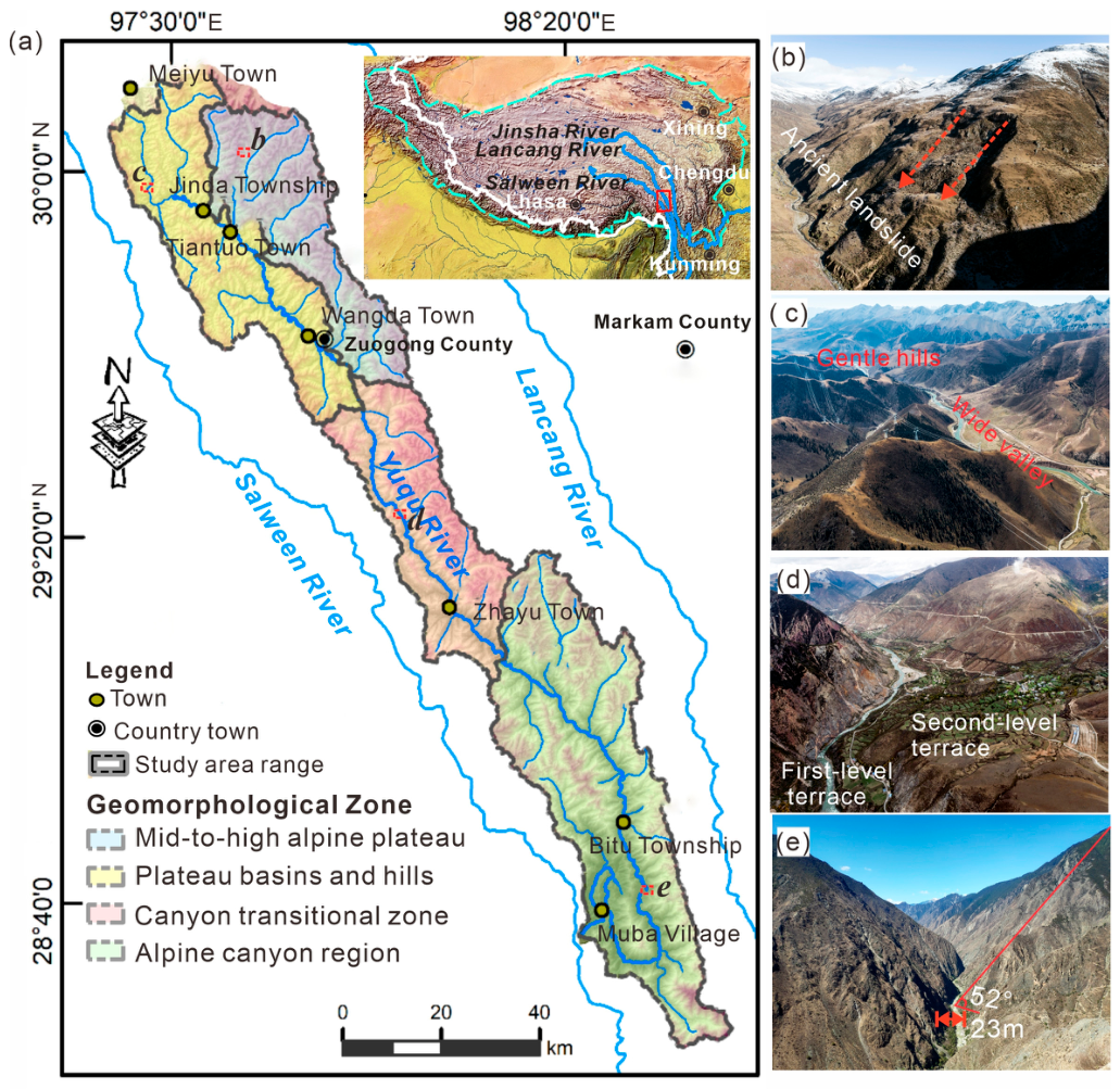
Figure 1.
Study area and geomorphological zones of the Yuqu River Basin: (a) location, drainage network, settlements, and geomorphological zoning; (b) plateau mountainous zone with an ancient landslide; (c) plateau wide-valley zone with gentle hillslopes and a broad valley floor; (d) transitional gorge zone with fluvial terraces; and (e) alpine gorge zone with a deeply incised valley and steep hillslopes.
Figure 1.
Study area and geomorphological zones of the Yuqu River Basin: (a) location, drainage network, settlements, and geomorphological zoning; (b) plateau mountainous zone with an ancient landslide; (c) plateau wide-valley zone with gentle hillslopes and a broad valley floor; (d) transitional gorge zone with fluvial terraces; and (e) alpine gorge zone with a deeply incised valley and steep hillslopes.
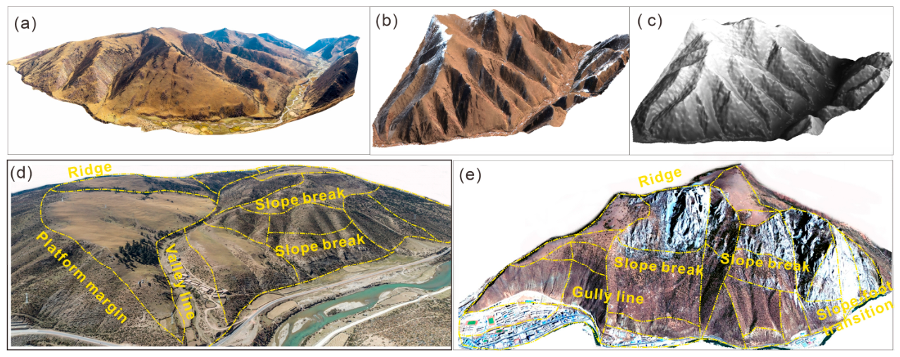
Figure 2.
Primary spatial datasets and representative expert-interpreted reference HTUs: (a) UAV orthomosaic; (b) Gaofen-2 image; (c) DEM-derived terrain representation on the 12.5 m working grid; (d) reference HTUs in the plateau wide-valley zone (yellow boundaries); and (e) reference HTUs in the alpine gorge zone (yellow boundaries).
Figure 2.
Primary spatial datasets and representative expert-interpreted reference HTUs: (a) UAV orthomosaic; (b) Gaofen-2 image; (c) DEM-derived terrain representation on the 12.5 m working grid; (d) reference HTUs in the plateau wide-valley zone (yellow boundaries); and (e) reference HTUs in the alpine gorge zone (yellow boundaries).
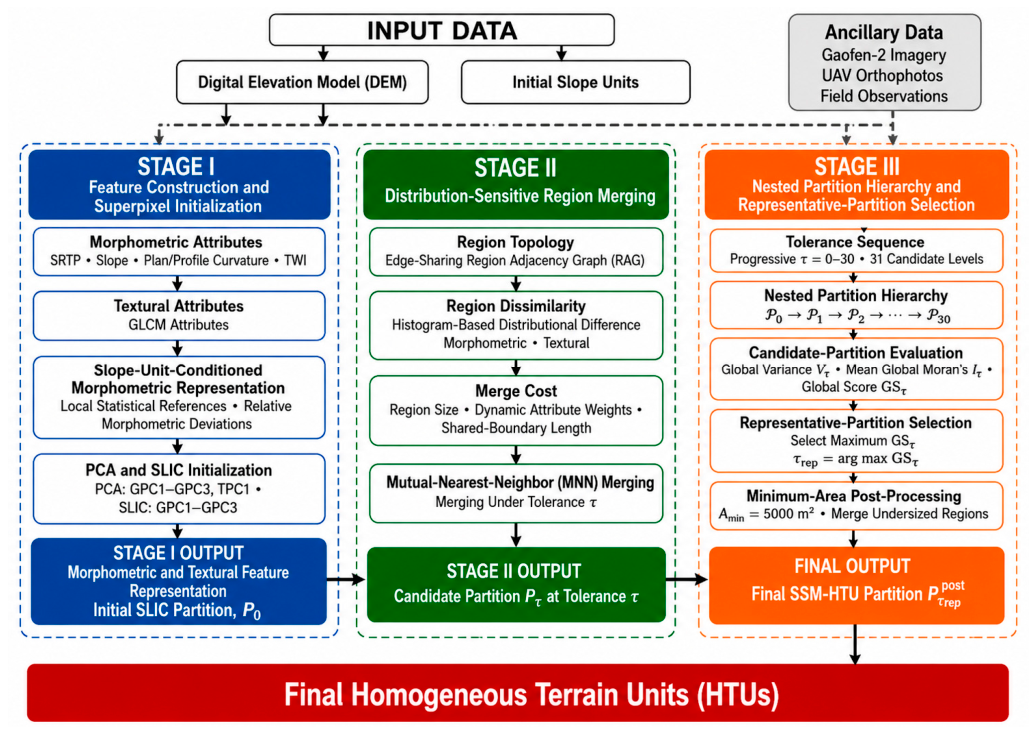
Figure 3.
Overall workflow of the SSM-HTU framework for homogeneous terrain-unit extraction.
Figure 3.
Overall workflow of the SSM-HTU framework for homogeneous terrain-unit extraction.
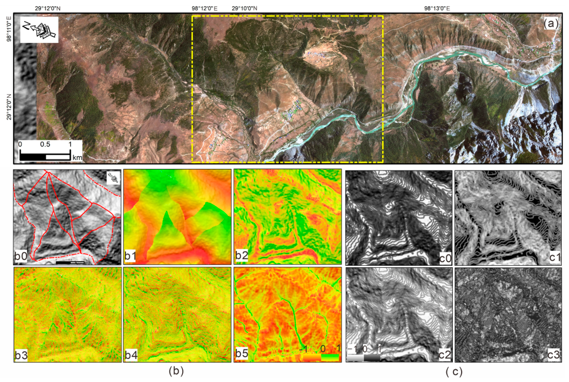
Figure 4.
Construction of the multidimensional terrain-attribute field: (a) optical image showing the representative terrain setting and selected demonstration area (yellow dashed box); (b) morphometric branch, comprising (b0) the initial slope units used as local statistical references and (b1–b5) the morphometric attributes, including slope-unit relative topographic position (SRTP), slope, plan curvature, profile curvature, and topographic wetness index (TWI); and (c) textural branch, comprising (c0–c3) representative GLCM-derived textural attributes, including angular second moment, contrast, inverse difference moment, and correlation. Red lines in panel (b0) delineate the initial slope-unit boundaries. The color gradients in panels (b1–b5) represent the spatial variation of the corresponding morphometric attributes, whereas grayscale intensity in panels (c0–c3) represents the corresponding textural attributes. Because the attributes have different physical meanings and value ranges, the graphical scales should be interpreted within individual panels.
Figure 4.
Construction of the multidimensional terrain-attribute field: (a) optical image showing the representative terrain setting and selected demonstration area (yellow dashed box); (b) morphometric branch, comprising (b0) the initial slope units used as local statistical references and (b1–b5) the morphometric attributes, including slope-unit relative topographic position (SRTP), slope, plan curvature, profile curvature, and topographic wetness index (TWI); and (c) textural branch, comprising (c0–c3) representative GLCM-derived textural attributes, including angular second moment, contrast, inverse difference moment, and correlation. Red lines in panel (b0) delineate the initial slope-unit boundaries. The color gradients in panels (b1–b5) represent the spatial variation of the corresponding morphometric attributes, whereas grayscale intensity in panels (c0–c3) represents the corresponding textural attributes. Because the attributes have different physical meanings and value ranges, the graphical scales should be interpreted within individual panels.

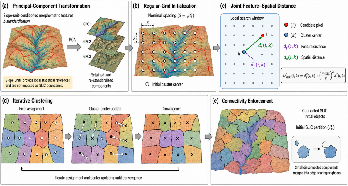
Figure 5.
Generation of the SLIC initial partition from the standardized morphometric principal component representation: (a) PCA of the standardized morphometric feature set and re-standardization of the retained GPC1–GPC3; (b) regular-grid initialization of cluster centers with nominal spacing S; (c) local evaluation of the joint feature–spatial distance; (d) iterative pixel assignment and cluster-center updating; and (e) connectivity enforcement to produce spatially connected SLIC initial objects constituting P0.
Figure 5.
Generation of the SLIC initial partition from the standardized morphometric principal component representation: (a) PCA of the standardized morphometric feature set and re-standardization of the retained GPC1–GPC3; (b) regular-grid initialization of cluster centers with nominal spacing S; (c) local evaluation of the joint feature–spatial distance; (d) iterative pixel assignment and cluster-center updating; and (e) connectivity enforcement to produce spatially connected SLIC initial objects constituting P0.
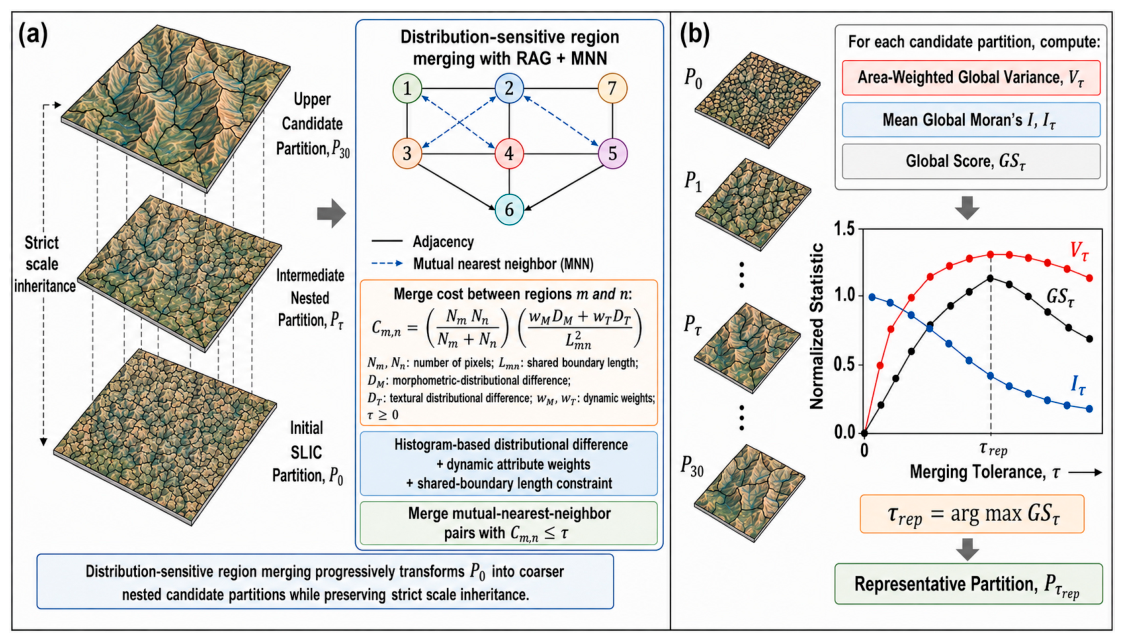
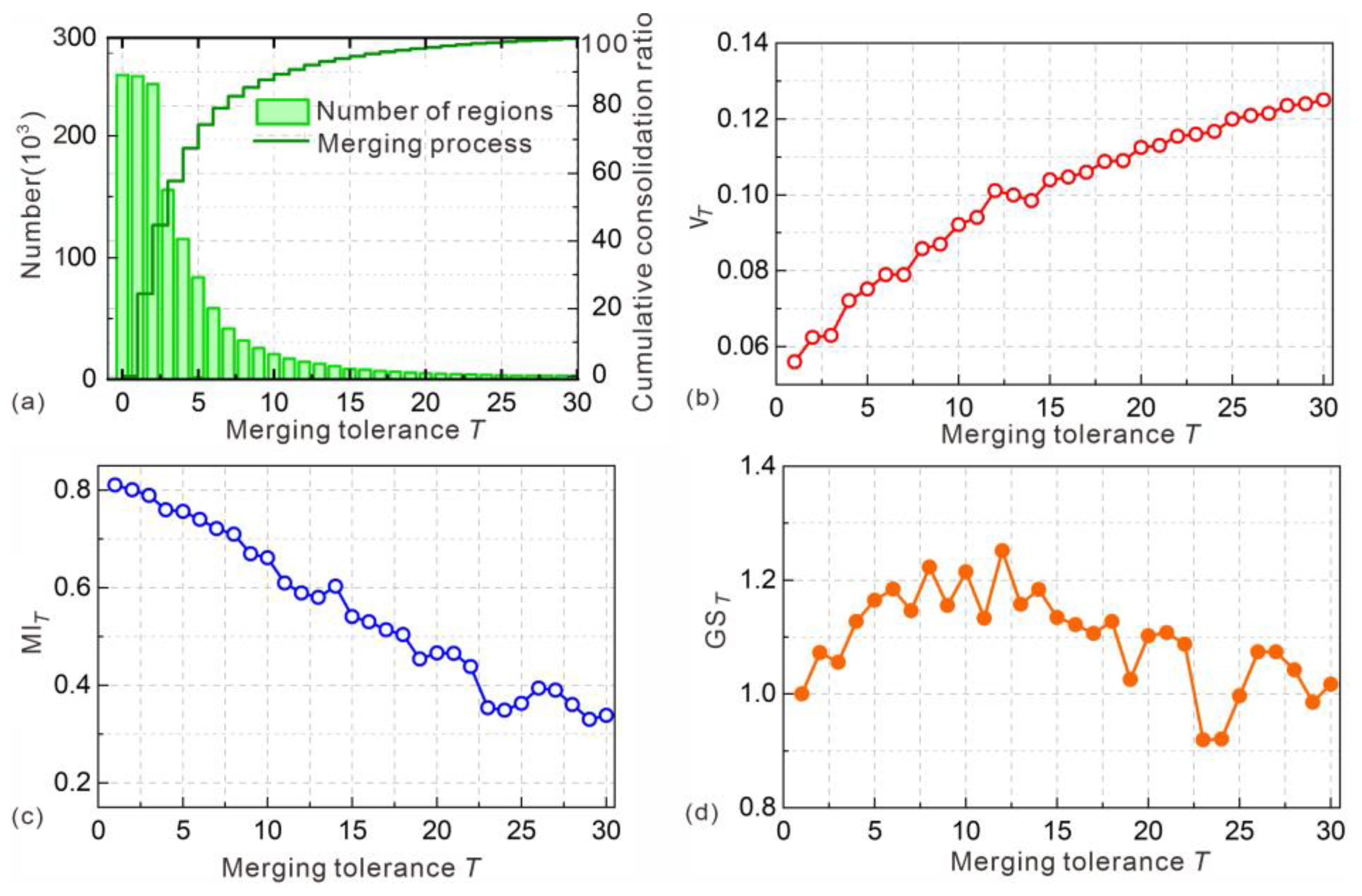
Figure 6.
Distribution-sensitive region merging, nested partition hierarchy, and representative-partition selection in SSM-HTU: (a) construction of the region adjacency graph (RAG), calculation of merge costs and mutual nearest neighbor (MNN) merging under tolerance τ, producing nested candidate partitions from P0 to P30; and (b) evaluation of candidate partitions using area-weighted Global Variance Vτ, mean Global Moran’s Iτ, and Global Score GSτ, with τrep = argmaxτ∈{0,…,30}GSτ defining the representative partition. Numbers 1–7 denote schematic identifiers of the example regions (graph nodes) in the RAG and have no quantitative meaning.
Figure 6.
Distribution-sensitive region merging, nested partition hierarchy, and representative-partition selection in SSM-HTU: (a) construction of the region adjacency graph (RAG), calculation of merge costs and mutual nearest neighbor (MNN) merging under tolerance τ, producing nested candidate partitions from P0 to P30; and (b) evaluation of candidate partitions using area-weighted Global Variance Vτ, mean Global Moran’s Iτ, and Global Score GSτ, with τrep = argmaxτ∈{0,…,30}GSτ defining the representative partition. Numbers 1–7 denote schematic identifiers of the example regions (graph nodes) in the RAG and have no quantitative meaning.
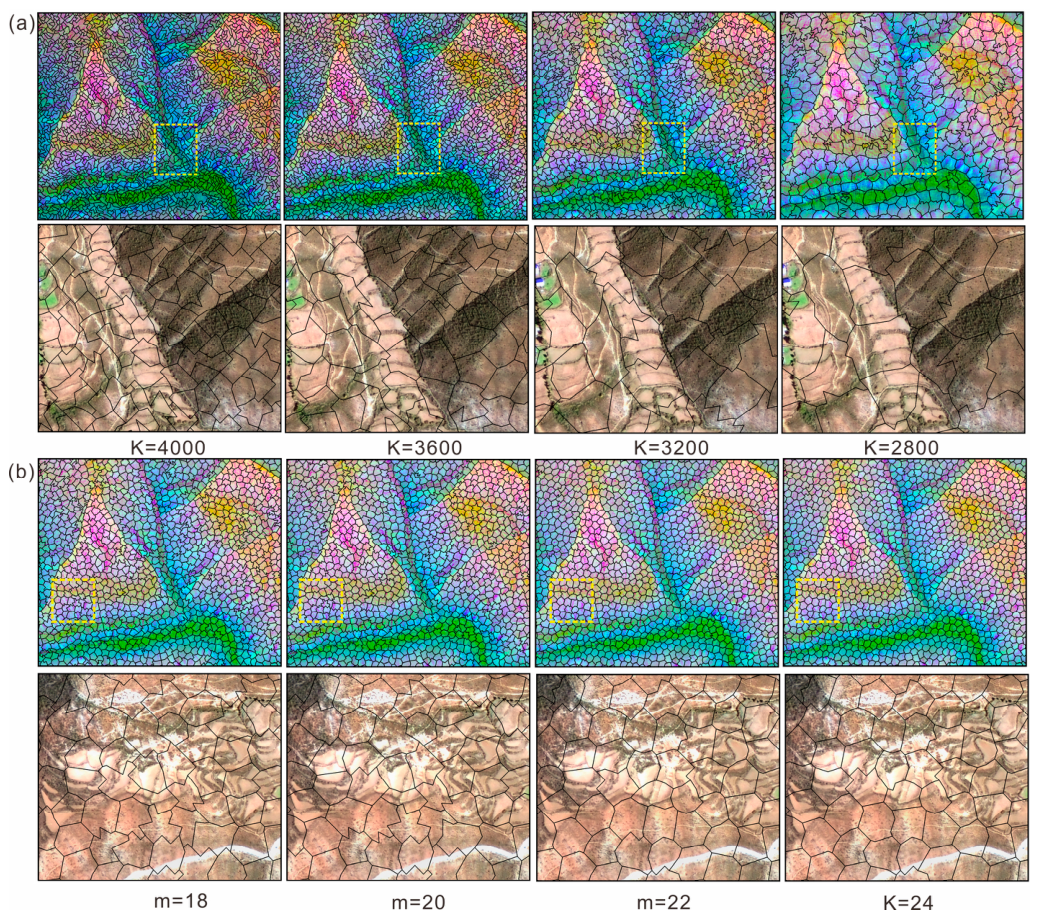
Figure 7.
Representative spatial effects of the sequential SLIC parameter calibration in one 700 × 700-pixel calibration window: (a) effects of K = 4000, 3600, 3200, and 2800 at the reference mSLIC = 22; and (b) effects of mSLIC = 18, 20, 22, and 24 at the selected K = 3200.
Figure 7.
Representative spatial effects of the sequential SLIC parameter calibration in one 700 × 700-pixel calibration window: (a) effects of K = 4000, 3600, 3200, and 2800 at the reference mSLIC = 22; and (b) effects of mSLIC = 18, 20, 22, and 24 at the selected K = 3200.
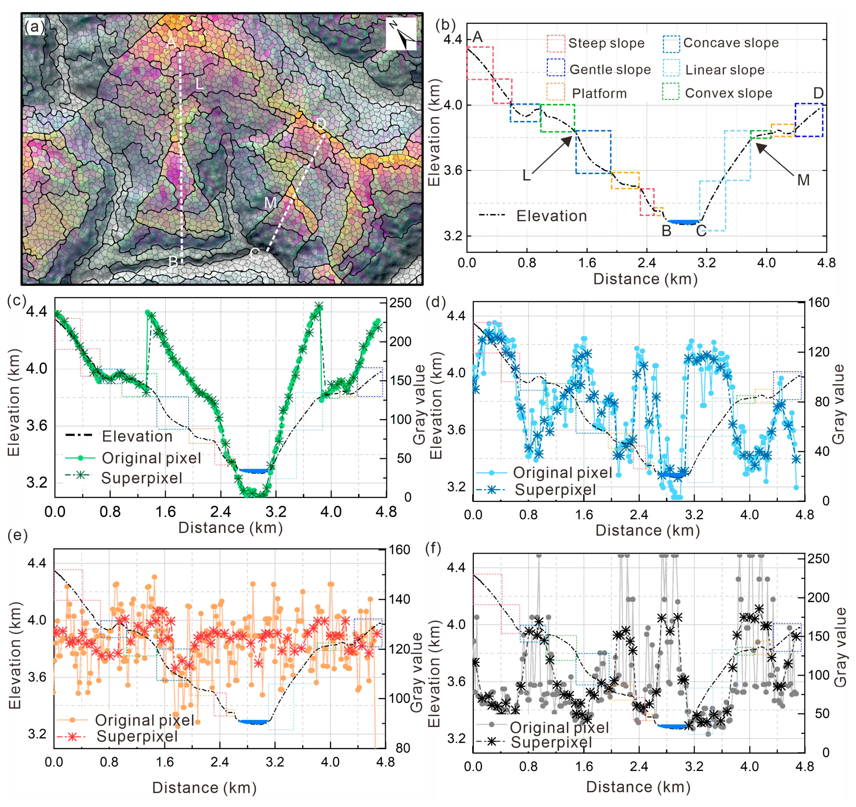
Figure 8.
Pixel-to-object transformation of the retained feature components along a cross-valley transect: (a) transect location over the SLIC partition; (b) elevation profile and visually interpreted terrain-form segments; and (c–f) pixel-level values and corresponding means within SLIC initial objects for GPC1, GPC2, GPC3, and TPC1. Labels A and D denote the two transect endpoints, whereas B, C, L, and M mark representative terrain-transition locations along the cross-valley profile; the same labels are used in panels (a,b) to indicate their spatial correspondence.
Figure 8.
Pixel-to-object transformation of the retained feature components along a cross-valley transect: (a) transect location over the SLIC partition; (b) elevation profile and visually interpreted terrain-form segments; and (c–f) pixel-level values and corresponding means within SLIC initial objects for GPC1, GPC2, GPC3, and TPC1. Labels A and D denote the two transect endpoints, whereas B, C, L, and M mark representative terrain-transition locations along the cross-valley profile; the same labels are used in panels (a,b) to indicate their spatial correspondence.
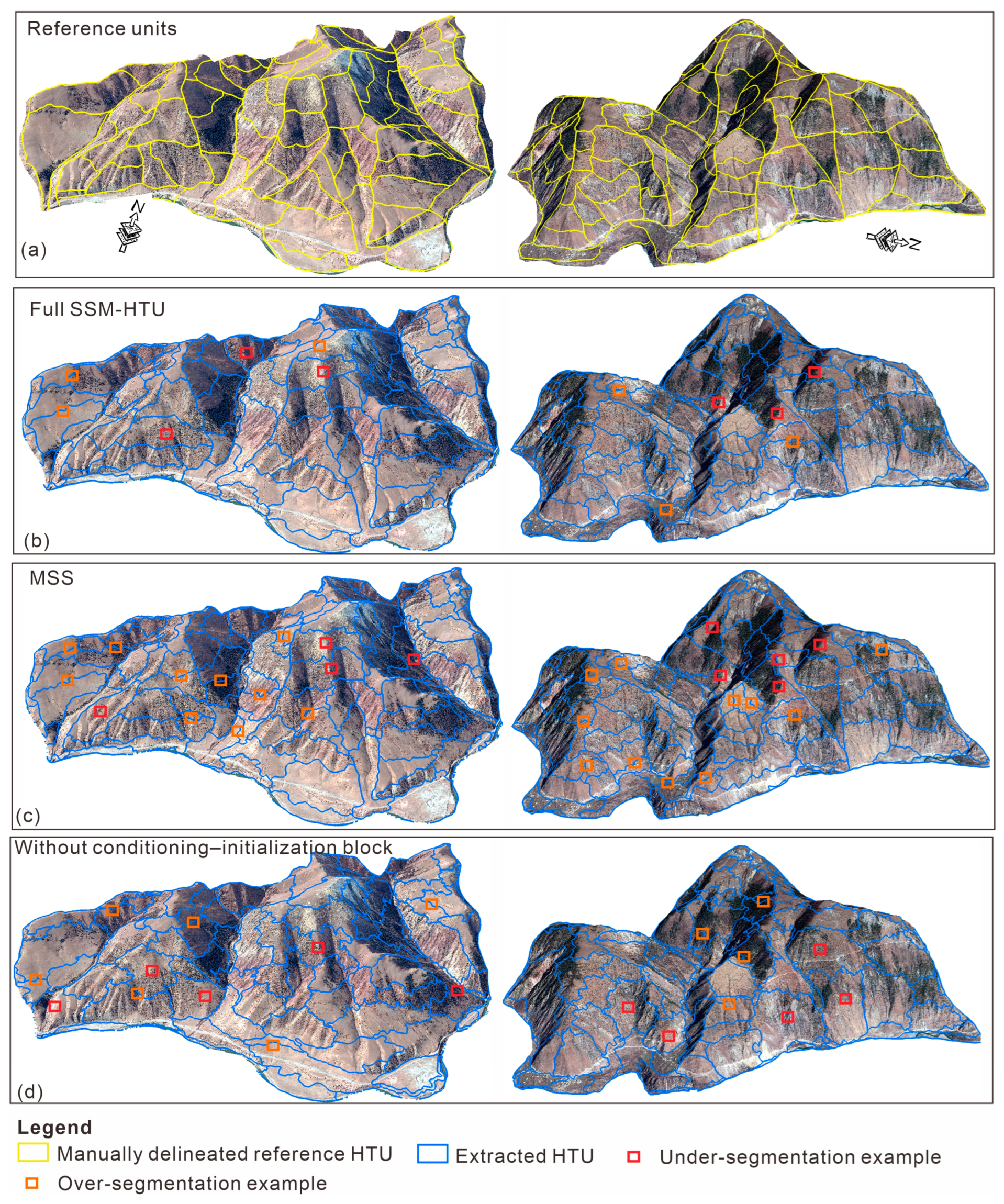
Figure 13.
Visual comparison of terrain-unit delineations in the plateau wide-valley zone (left) and alpine gorge zone (right): (a) expert-interpreted reference HTUs; (b) Full SSM-HTU; (c) MSS baseline; and (d) SSM-HTU without the conditioning–initialization block.
Figure 13.
Visual comparison of terrain-unit delineations in the plateau wide-valley zone (left) and alpine gorge zone (right): (a) expert-interpreted reference HTUs; (b) Full SSM-HTU; (c) MSS baseline; and (d) SSM-HTU without the conditioning–initialization block.
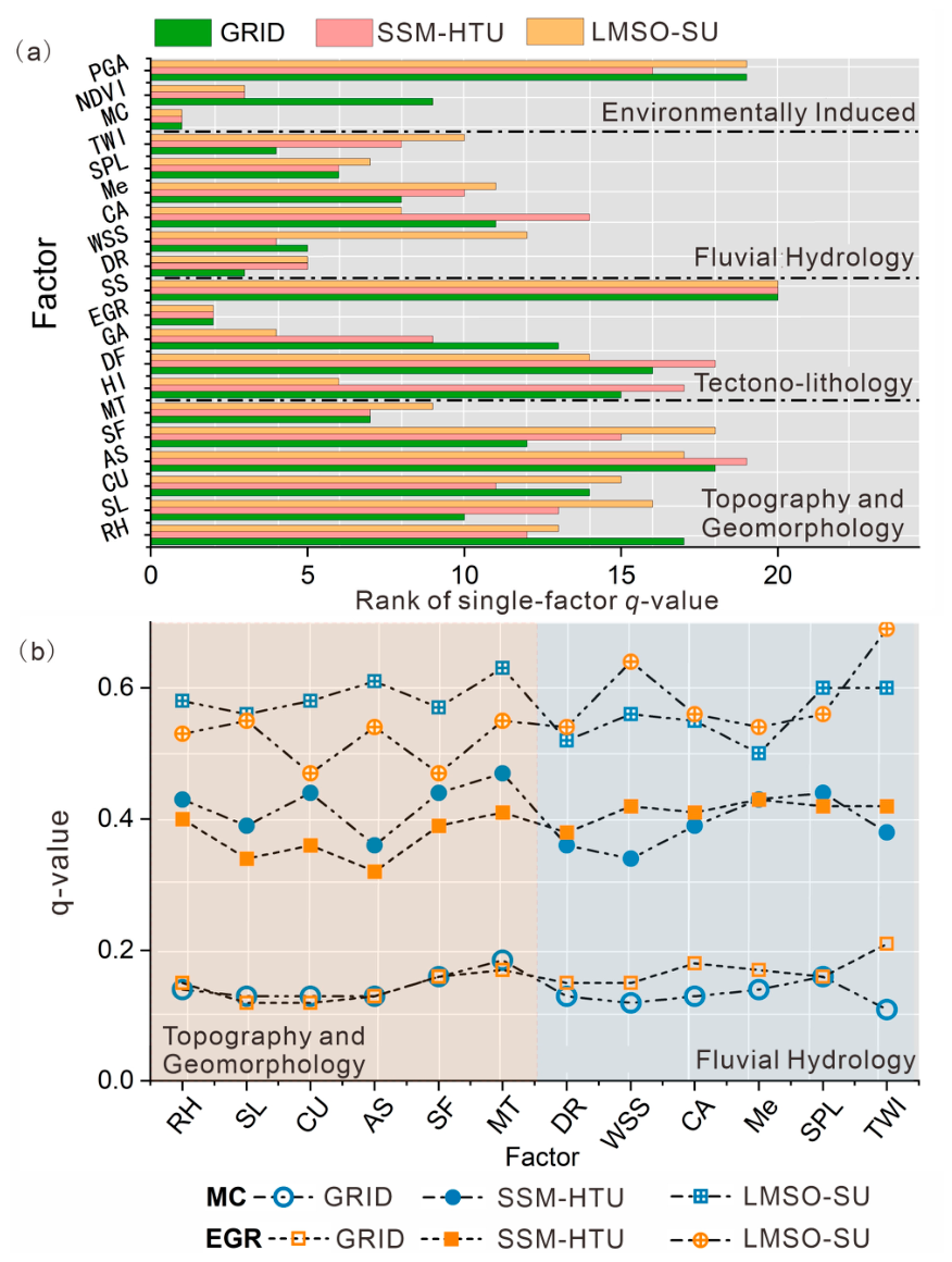
Figure 14.
Geodetector-based spatial associations under the three mapping-unit schemes: (
a) relative ranks of single-factor
q-values for the 20 conditioning factors; and (
b) representative interaction
q-values of MC and EGR with selected topographic–geomorphological and fluvial–hydrological factors. Background shading distinguishes the two factor groups. Factor abbreviations are defined in
Supplementary Table S1.
Figure 14.
Geodetector-based spatial associations under the three mapping-unit schemes: (
a) relative ranks of single-factor
q-values for the 20 conditioning factors; and (
b) representative interaction
q-values of MC and EGR with selected topographic–geomorphological and fluvial–hydrological factors. Background shading distinguishes the two factor groups. Factor abbreviations are defined in
Supplementary Table S1.
Table 1.
Explained and cumulative variances of the principal components retained in the morphometric and textural branches.
Table 1.
Explained and cumulative variances of the principal components retained in the morphometric and textural branches.
| Feature Branch | Principal Component | Explained Variance | Cumulative Explained Variance |
|---|
| Morphometric | GPC1 | 0.51 | 0.51 |
| GPC2 | 0.25 | 0.76 |
| GPC3 | 0.14 | 0.90 |
| Textural | TPC1 | 0.91 | 0.91 |
Table 2.
First-stage sensitivity to the requested number of SLIC clusters K across four geomorphological zones at the reference mSLIC = 22. Values are means ± standard deviations across four 700 × 700-pixel calibration windows.
Table 2.
First-stage sensitivity to the requested number of SLIC clusters K across four geomorphological zones at the reference mSLIC = 22. Values are means ± standard deviations across four 700 × 700-pixel calibration windows.
| K | Boundary Recall (12.5 m Tolerance) | Under-Segmentation Error | Mean Superpixel Area (m2) |
|---|
| 2800 | 0.858 ± 0.027 | 0.123 ± 0.018 | 27,500 ± 1200 |
| 3200 | 0.879 ± 0.024 | 0.106 ± 0.016 | 24,000 ± 1000 |
| 3600 | 0.886 ± 0.022 | 0.099 ± 0.015 | 21,300 ± 900 |
| 4000 | 0.891 ± 0.021 | 0.094 ± 0.014 | 19,200 ± 800 |
Table 3.
Second-stage sensitivity to the SLIC compactness parameter mSLIC across four geomorphological zones at the selected K = 3200. Values are means ± standard deviations across four 700 × 700-pixel calibration windows.
Table 3.
Second-stage sensitivity to the SLIC compactness parameter mSLIC across four geomorphological zones at the selected K = 3200. Values are means ± standard deviations across four 700 × 700-pixel calibration windows.
| mSLIC | Boundary Recall (12.5 m Tolerance) | Under-Segmentation Error | Mean Superpixel Area (m2) |
|---|
| 18 | 0.883 ± 0.030 | 0.102 ± 0.021 | 23,900 ± 1050 |
| 20 | 0.882 ± 0.027 | 0.104 ± 0.019 | 23,950 ± 1020 |
| 22 | 0.879 ± 0.024 | 0.106 ± 0.016 | 24,000 ± 1000 |
| 24 | 0.873 ± 0.025 | 0.112 ± 0.018 | 24,050 ± 1010 |
Table 4.
Terrain-unit characteristics and geometric performance of the final SSM-HTU partition across four geomorphological zones.
Table 4.
Terrain-unit characteristics and geometric performance of the final SSM-HTU partition across four geomorphological zones.
| Geomorphological Zone | No. of Reference Units | No. of Final HTUs | Median Unit Area (km2) | Area-Weighted IoU | Boundary F1 (12.5 m Tolerance) |
|---|
| Plateau wide-valley zone | 165 | 9297 | 0.1627 | 0.724 | 0.709 |
| Plateau mountainous zone | 126 | 7101 | 0.1630 | 0.705 | 0.689 |
| Transitional gorge zone | 130 | 7127 | 0.1725 | 0.671 | 0.651 |
| Alpine gorge zone | 259 | 13,589 | 0.1885 | 0.688 | 0.674 |
| Overall | 680 | 37,114 | 0.1743 | 0.6945 | 0.6810 |
Table 5.
Partition characteristics and geometric performance of the MSS baseline and SSM-HTU configurations at approximately comparable partition granularity.
Table 5.
Partition characteristics and geometric performance of the MSS baseline and SSM-HTU configurations at approximately comparable partition granularity.
| Method | Unit Count | Median Area (km2) | Precision | Recall | Area-Weighted IoU | Mean Unweighted IoU | Boundary F1 (12.5 m Tolerance) |
|---|
| MSS baseline | 36,583 | 0.1830 | 0.8432 | 0.7615 | 0.6710 | 0.5560 | 0.5980 |
| Full SSM-HTU | 37,114 | 0.1743 | 0.8340 | 0.8011 | 0.6945 | 0.6180 | 0.6810 |
| Without conditioning–initialization block | 38,351 | 0.1569 | 0.8460 | 0.7750 | 0.6830 | 0.5830 | 0.6320 |
| Mean-based SSM-HTU | 37,463 | 0.1708 | 0.8405 | 0.7920 | 0.6900 | 0.6040 | 0.6620 |
Table 6.
Mapping-unit characteristics and landslide-response sample structures for the three spatial-support schemes.
Table 6.
Mapping-unit characteristics and landslide-response sample structures for the three spatial-support schemes.
| Mapping Scheme | Total Units, N | Mean Unit Area (km2) | Positive Units, N+ | Negative Units, N− | Positive-Unit Prevalence (%) |
|---|
| GRID, 30 m | 5,706,667 | 0.0009 | 18,200 | 5,688,467 | 0.319 |
| LMSO-SU | 6572 | 0.7815 | 840 | 5732 | 12.78 |
| SSM-HTU | 37,114 | 0.1384 | 1520 | 35,594 | 4.10 |
Table 7.
Summary of factor-detector, interaction-detector, and risk-detector results under the three mapping-unit schemes.
Table 7.
Summary of factor-detector, interaction-detector, and risk-detector results under the three mapping-unit schemes.
| Mapping Scheme | No. of Factors with q > 0.1 | Mean Single-Factor q | Maximum Interaction q | No. of Interactions with q > 0.6 | No. of Factors with ≥1 Unadjusted Pairwise Contrast |
|---|
| GRID | 0 | 0.04 | 0.22 | 0 | 6 |
| SSM-HTU | 12 | 0.14 | 0.69 | 9 | 12 |
| LMSO-SU | 10 | 0.13 | 0.67 | 6 | 16 |



 ,
,