Deep Learning for Water Body Segmentation in Remote Sensing Imagery: A Review

Highlights
- This review summarizes recent deep learning architectures for water body segmentation in remote sensing imagery, including U-Net, DeepLabv3+, Transformer, Mamba, and SAM-based models. A neural network is proposed for covariance-mismatch-tolerant phase-only beamforming.
- It also reviews commonly used water body datasets and evaluation metrics, and discusses current challenges and future research directions.
- This review provides a structured reference for selecting, comparing, and improving deep learning models for water body segmentation.
- It offers practical guidance for dataset selection, metric evaluation, and future methodological development in remote sensing water body segmentation.
Abstract
1. Introduction
2. Methods for Literature Search and Screening
3. Deep Learning-Based Water Body Segmentation Methods
3.1. Water Body Segmentation Models Based on the U-Net Model
3.1.1. Improvements to Encoder Structure
- Introduce an attention mechanism: To address unstable spectral reflectance- and reflection-induced interference in multispectral water body segmentation, Hu et al. [35] embedded a channel attention mechanism in each encoder stage. Compared with the standard U-Net, this approach strengthens channel-wise feature representation. The spatial branches not only extract shapes and boundaries but also adaptively recalibrate responses across spectral bands. Wang et al. [36] integrated a Transformer-based multi-head attention module after the U-Net encoder, enabling the joint modeling of image features across multiple subspaces and improving the model ability to identify flood-related characteristics. The AER U-Net model proposed by Jonnala et al. [37] reduces skip connection complexity by introducing a self-attention module. For water body segmentation, this architecture enables effective discrimination between water and non-water regions.
- Optimize the convolutional layer: Zhang et al. [38] reported that D-UNet has a smaller receptive field. By replacing standard convolutions with multiscale dilated convolution modules, they enhanced feature extraction and segmentation accuracy, reducing missed detections and false positives. Many deep learning networks for water extraction rely on the translation invariance of convolution kernels, Xu et al. [39] introduced rotation-invariant convolutions within a U-Net framework to refine the architecture and enrich internal representations, enabling the robust recognition of water bodies under image rotation. To better model complex channel relationships in RGB imagery, Wang et al. [40] replaced conventional convolutional blocks with quaternion convolutions, which learn optimal weighting across the RGB channels and improve multiscale water body recognition.
- Changes in the backbone network: Wagner et al. [41] used ResNeXt 50 as the backbone of a U-Net model and compared 32 CNN architectures for water body segmentation. The results indicate that the improved model achieved the best segmentation performance and can be used for the real-time monitoring of river water levels. To improve water body segmentation accuracy, Liu et al. [42] replaced the VGG module in U-Net with MobileNetV2 and leveraged the inverted residual structure and the linear bottleneck layer of MobileNetV2 to efficiently extract spatial features and improve water body segmentation performance. Xia et al. [43] further lightweighted U-Net by reducing the number of convolutional kernels per layer from 64–1024 to 32–512, decreasing the parameter count to approximately one quarter of the original while maintaining essentially unchanged segmentation accuracy.
- Other improvements: Li et al. [44] proposed the GLF-MFUNet model for Sentinel-2 satellite imagery. The dual-path encoder extracts global and local features in parallel, which helps to capture local details and global contextual information and achieves strong performance in small-target water body segmentation. Cai et al. [45] improved the U-Net architecture by incorporating an image upsampling module to form a symmetric structure and further deepen the network via an “S”-shaped loop design. Their results indicate improved water body segmentation accuracy under complex backgrounds.
3.1.2. Improving Skip Connections
3.1.3. Decoder Structure Optimization
3.1.4. Summary of Improvements Based on the U-Net Model
3.2. Water Body Segmentation Models Based on the DeepLabv3+ Model
3.2.1. Improvements to Encoder Structure
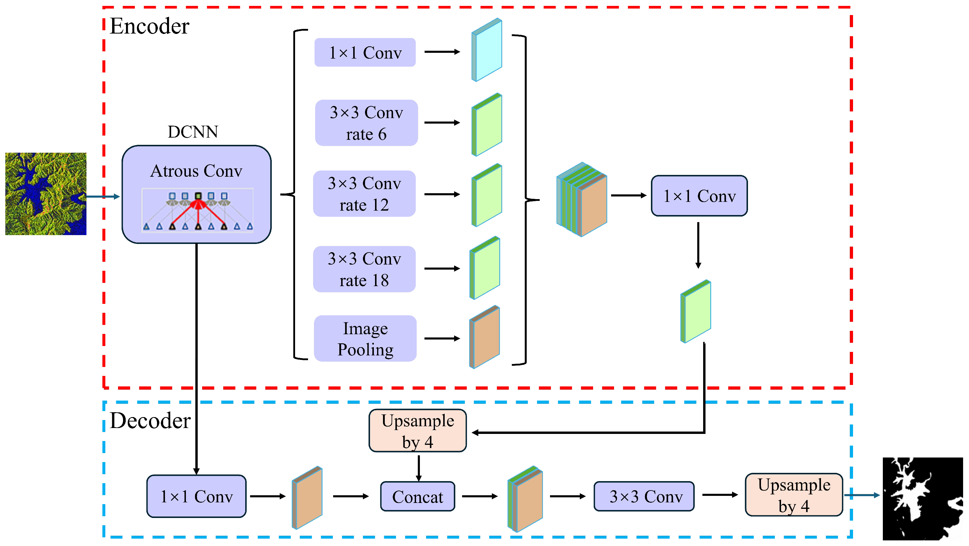
- Optimize the ASPP module: Luo et al. [59] optimized the ASPP module in DeepLabv3+. Compared with the square pooling kernels used in the original model, the introduced strip pooling kernels are better suited for extracting scattered distribution water bodies over long ranges. Zhang et al. [60] introduced two modifications to the ASPP module in the encoder. The dilation rates were adjusted from 6, 12, and 18 to 2, 4, 8, and 16; this adjustment is more advantageous for capturing feature information from elongated rivers. The standard convolution in the ASPP module was replaced with depthwise separable convolution, which reduces the number of model parameters and improves training efficiency. During water body segmentation, when the river surface and its surrounding environment change, the ASPP module may not adapt well to such target variation. Therefore, Sun et al. [61] restructured the ASPP module as a densely connected DASPP module. In this design, the dilation rate is increased progressively, and dense connections allow upper-layer atrous convolutions to reuse the outputs of lower-layer atrous convolutions. This strategy expands the receptive field and enables multiscale feature extraction. Compared with the original ASPP module, the DASPP module improves water body segmentation accuracy.
- Changes in the backbone network: Huang et al. [62] employed an enhanced DeepLabv3+ model to segment black and odorous water in Gaofen-2 remote sensing imagery. Compared to DeepLabv3+, they replaced the original backbone network with MobileNetV2. This modification reduced the model size from 226 MB to 23.3 MB. Xue et al. [63] also adopted MobileNetV2 as the backbone network for urban waterlogging monitoring. Zhang et al. [64] employed ResNet101 as the backbone network of DeepLabv3+ to segment duckweed-type black and odorous water. This design mitigated vanishing and exploding gradients while enhancing model generalization. Chen et al. [65] incorporated Swin Transformer as an additional backbone network in DeepLabv3+. In this configuration, the same remote sensing image is fed into two backbone networks to generate feature maps. The output features from the two parallel backbones are then upsampled and fused to enable the recognition and segmentation of specular water bodies on the land surface.
3.2.2. Decoder Structure Optimization
3.2.3. Summary of Improvements Based on the DeepLabv3+ Model
3.3. Water Body Segmentation Models Based on Transformer Models
3.4. Water Segmentation Based on a Hybrid Model Combining Transformers and CNN
3.4.1. Embedding Transformers into CNN
3.4.2. Parallel Hybrid Structure
3.4.3. Transformer Feature Enhancement—CNN Feature Extraction
3.4.4. Transformer Encoder—CNN Decoder
3.4.5. Summary Table of Improvements in Hybrid Transformer and CNN Models
3.5. Water Body Segmentation in the Mamba Model
3.6. Water Body Segmentation Based on the SAM Model
3.7. Summary of Water Body Segmentation Models
4. Water Body Segmentation Dataset and Evaluation Metrics
4.1. Water Body Segmentation Dataset
4.2. Evaluation Metrics
5. Challenges and Outlook
5.1. Existing Challenges
- Challenges in Extracting Small and Fragmented Water Bodies: Pixels corresponding to small and fragmented water bodies usually constitute only a small proportion of remote sensing imagery and provide limited discriminative information. During model downsampling, these weak cues are attenuated or lost, which impairs reliable detection. As a result, spatially continuous water features, such as narrow streams, may be segmented into disconnected fragments, yielding scattered outputs that resemble short line segments or even isolated points and thus exhibit pronounced fragmentation. Small water bodies reflect the same underlying challenge, namely, the limited spatial extent of the targets. Current methods still provide insufficient feature extraction for small water bodies, particularly for accurate boundary delineation.Although extracting small targets from fragmented water bodies remains highly challenging, it is critical to human survival [106,107]. Considerable efforts have therefore been devoted to addressing this problem. Previous studies have shown that the modified normalized difference water index, calibrated for small reservoirs with areas ranging from 1 to 10 ha, exhibits high threshold stability and can reduce false negative predictions caused by shallow water and submerged vegetation. However, this method cannot completely prevent the loss of information at the subpixel scale [108]. Various deep learning methods have recently been proposed as promising solutions to this challenge. Qin et al. applied U-Net to extract small water bodies from hyperspectral imagery. By exploiting spectral differences within the imagery, their method enhanced the discrimination between water bodies and background features and used skip connections to transfer detailed information from shallow feature layers to the decoder. Nevertheless, repeated downsampling may still reduce the segmentation accuracy of narrow water bodies [109]. WaterNet is a novel deep CNN that incorporates concepts from Gaussian filtering and edge detection into a dual residual refinement module for segmenting small water bodies [110]. In addition, the AWS16K dataset, which was developed by comprehensively considering sample coverage across different regions, water body types, and complex backgrounds, provides an effective supplementary resource for improving small water body segmentation [111]. Despite these advances, further progress is needed to overcome the limitations of traditional methods, account for variability across acquisition times and seasons, balance temporal and spatial resolution, and improve the interpretability of deep learning models to better satisfy real-world application requirements.
- Misjudgments and Missed Judgments in Complex Scenarios: Misclassification and omission in surface water body segmentation are primarily caused by the combined effects of spectral similarity between classes, spectral variability within classes, and mixed pixels. Spectral similarity between different objects occurs when water bodies exhibit spectral responses similar to those of shadows, dark roads, or saline and alkaline land. Spectral variability within the same object occurs when a single water body displays different spectral signatures because of variations in water depth, turbidity, sun glint, or season. Mixed pixels, by contrast, result from the limited spatial resolution of the sensor. When a single pixel contains water, vegetation, soil, or buildings simultaneously, its observed spectrum can be approximated as the sum of the spectra of these components weighted by their respective area proportions.Distinguishing different objects with similar spectral responses from the same objects with variable spectral responses remains a major challenge in land and sea segmentation. To address data diversity and the lack of prior information, some studies have introduced additional encoding branches into end-to-end PMFormer architectures and employed deep clustering to capture substantial spectral variability within classes [112]. Saline and alkaline land is particularly difficult to distinguish from water because of their similar spectral characteristics. Using Lake Aibi in the Xinjiang Uygur Autonomous Region as a case study, researchers incorporated a saline and alkaline land endmember into a spectral mixing framework with multiple endmembers and dynamically selected thresholds according to image histogram characteristics, thereby improving the separability of water bodies from saline and alkaline land [113]. For urban water body segmentation, an initial water mask can be generated using the normalized difference water index and the Otsu threshold, followed by morphological dilation to identify mixed pixels [114]. In mapping below the pixel scale, DE_MRF applies both dilation and erosion to identify potential mixed pixels inside and outside water body boundaries and represents spectral variation within classes using multiple local water and land endmembers [115]. Other studies have used CNN to learn the relationship between local seawater background components and algal components and then adjusted the Otsu threshold according to differences in coverage before and after deconvolution. This approach provides a basis for feedback calibration with mixed pixels along water body boundaries [116]. More recently, methods for increasing spatial resolution have been applied to reduce spectral mixing along river boundaries and estimate the proportion of water within mixed pixels [117]. Despite this progress, the spatial distribution of water within mixed pixels cannot yet be characterized with sufficient accuracy. Moreover, many existing methods depend heavily on imagery with high spatial resolution, and irregular water bodies with nonstationary characteristics remain insufficiently investigated.
- The Scarcity and Cost of High-quality Annotated Data: Deep learning model training depends critically on adequate samples; however, data availability for water body segmentation remains limited. Pixel-level annotations are particularly scarce for elongated rivers and small ponds, and high-quality labels that remain representative across regions, seasons, and terrain conditions are still lacking. In addition, existing datasets are often strongly imbalanced: annotated samples are concentrated on large water bodies, such as rivers, lakes, and reservoirs, whereas samples for small water bodies are comparatively limited. These constraints can substantially hinder the generalization of water body segmentation models.Training with manually annotated data is highly time consuming [118]. Facing the scarcity of high-quality annotated data, transfer learning has emerged as a practical alternative. For example, transfer learning can be incorporated into Siamese network architectures to reduce the dependence on labeled data. It can also be used to train water body segmentation models and thereby alleviate performance degradation caused by limited annotations. A two-stage transfer learning strategy has also been reported, in which models are pretrained on Sentinel-2 imagery and then fine-tuned on PlanetScope data to transfer spectral representations and reduce labeling costs [119,120,121]. Although these approaches generally reduce reliance on high quality annotations, they remain subject to limitations, including sensitivity to natural factors such as occlusion and illumination, as well as challenges associated with heterogeneous remote sensing imagery. Further research is needed to address these issues in a systematic manner.
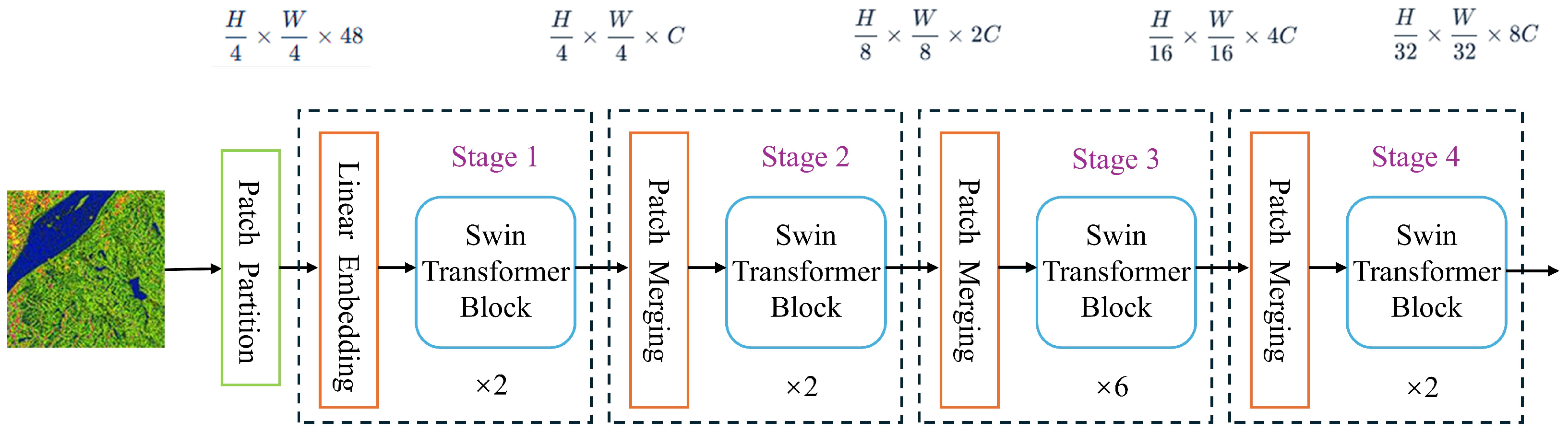
- The Challenge of Generalization Across Seasons and Cross-Regional Scenarios: Seasonal variation, temporal consistency, regional transferability, and generalization across sensors remain major challenges in water body segmentation. Water bodies exhibit substantial morphological differences across geographic regions and seasonal conditions, such as between humid plains and arid mountainous areas, between wet and dry seasons, and between snow- and ice-covered winter landscapes and vegetation covered summer landscapes. These variations can markedly reduce model robustness and transferability. In addition, differences in spatial resolution, spectral response, and imaging mechanisms constrain generalization across sensors. Consequently, achieving reliable performance across seasons, regions, and sensor types remains an unresolved challenge.A contrastive learning module was incorporated into SAM to align features across synthetic images, enabling robust water body segmentation across regions without requiring annotated data [122]. Conventional methods based on thresholding or supervised classification often require thresholds or training samples to be adjusted for different regions and sensors. By contrast, a large-scale framework for water body segmentation across sensors was developed using unsupervised deep learning. This framework exploits the physical and spatial characteristics of water bodies to automatically distinguish and collect diverse samples, achieving strong overall performance across different sensor types [123]. Because lakes exhibit distinct spectral characteristics in winter and summer, a method combining K means clustering with flood fill was proposed. By selecting appropriate metrics and removing small objects along lake boundaries, this method improved the temporal continuity, accuracy, and stability of lake extraction [124]. To accurately segment areas subject to seasonal flooding, researchers developed a harmonic model based on long-term time-series dynamics of surface water. The amplitude derived from the harmonic model was used to characterize the frequency of transitions between land and water, resulting in high accuracy and robustness [125]. Lakes also undergo transitions between periods with and without ice because of seasonal variation, and conventional spectral indices and machine learning methods remain limited in distinguishing these conditions. To address this issue, large language models were combined with random forest algorithms to generate candidate indices for distinguishing water, ice, and snow. The optimal ERNIE WISI index was then selected to automatically classify water, ice, and snow without requiring seasonal threshold adjustment [126]. Despite these advances, differences in temporal dynamics caused by climatic variability and the limited generalization of models under extreme conditions or in specific geographic environments remain unresolved.
5.2. Future Research Directions
- Spatiotemporal Adaptive Multimodal Fusion: Recent studies have incorporated multi-source remote sensing data for water body segmentation. For instance, Sentinel-1 data have been used to complement information missing in Sentinel-2 imagery [127]; SAR data and digital elevation models have been integrated for flood mapping [128]; and a combination of Landsat-8 and Landsat-9 with Sentinel-1 and Sentinel-2 has been applied to estimate irrigated areas in the Delingha piedmont grasslands of northwestern China [129]. Although these efforts have yielded promising results, most existing methods still rely on a single remote sensing image and often neglect multi-temporal information. Multisource data provide complementary cues for water delineation, reduce the effects of cloud cover and illumination variability, improve spatial resolution, and offer stronger robustness in complex scenes. Multi-temporal data identify the variation of periodic water dynamics and facilitate discrimination between persistent water bodies and short-term inundation, while improving the monitoring of extreme events such as floods and dam failures. Despite the clear benefits of combining multisource and multi-temporal data, further methodological improvements remain necessary. Future research is expected to move beyond conventional multimodal fusion toward spatial, temporal, and feature adaptivity. Multisource data, including optical imagery, SAR imagery, thermal infrared imagery, digital elevation models, historical time series data, LiDAR point clouds, and related sources, may be selected adaptively according to application scenarios and integrated through fusion networks with dynamic weighting. These advances are expected to improve discrimination of fine-grained water bodies.
- Segmentation Strategies for Large Model Integration: General-purpose vision foundation models, represented by the SAM series, have attracted considerable attention in water body segmentation and are increasingly being applied in this field. The Prithvi-EO series [130] and SeaMo [131] have also been introduced for water body segmentation, and related studies are currently emerging. Although TerraMind [132], SkySense [133], and SpectralGPT [134] have not yet been specifically investigated for water body segmentation, they already possess the multimodal and cross-domain representation capabilities required for this task. However, these models remain dependent on prompts and do not fully address the challenges associated with domain shift; consequently, their cross-domain generalization performance remains unstable. With ongoing advances in science and technology, requirements for integrating large-scale foundation models are expected to become more stringent. The scope is expected to extend beyond water body delineation to forecast future dynamics, such as changes in drought- and flood-affected areas. For task-specific models, a direction is the development of geospatial foundation models that generalize across seasons and regions, thereby improving generalization and zero-shot capability. In addition, reducing parameter counts and applying model compression to support lightweight deployment are likely to remain priorities for future research.
- Fine-grained Water Body Segmentation: Current water body segmentation methods largely remain at the level of holistic detection and lack the capability for fine-grained segmentation. This is because they fail to account for intrinsic differences in water type and composition that commonly coexist within a single water body, such as clear water, polluted water, and areas dominated by aquatic vegetation. Since these distinct water types require different management strategies and have varied environmental impacts, conventional pixel-level segmentation—which does not provide water type information—can lead to inaccurate parameterization in Earth system models, including those for water quality, ecological assessment, hydrology, and climate. To address contemporary application needs, it is essential to move beyond binary water classification. Fine-grained water body segmentation can not only delineate water extent more precisely but also support the prediction of water evolution, retrieval of water quality parameters, and identification of periodic variations in water type. Furthermore, it enables interdisciplinary applications and provides critical support for climate research, fisheries management, and water resources planning. Future research is expected to advance toward finer water body segmentation, with emphasis on pixel-level boundary delineation and the retrieval of higher-level water body-related semantics and parameters. This shift moves beyond locating water bodies toward identifying water types, enabling a more refined semantic segmentation of turbid waters, black and malodorous waters, aquatic vegetation-covered waters, shadow-affected waters, and ice surfaces. These advances are expected to promote a transition from perception to cognition and thereby better utilize effective water resource use. To achieve more precise water body segmentation, future studies could incorporate neural networks informed by physical principles to constrain the transport, diffusion, and decay of pollutants, suspended matter, and chlorophyll along flow fields. In addition, shallow water equations or shoreline kinematic conditions could be used to constrain variations in water body boundaries. On this basis, a joint representation framework could be developed to delineate water body boundaries while simultaneously predicting semantic categories, such as clear and turbid water, or estimating continuous parameters, including chlorophyll a concentration, suspended solids concentration, and turbidity.
- Integration of Explainability and Physical Mechanisms: Although recent improvements in water body segmentation models have enhanced segmentation performance, the mechanisms underlying these gains remain insufficiently understood. Moreover, when models are applied to imagery acquired at different spatial resolutions or by different sensors, nonlinear variations in segmentation accuracy cannot be explained solely by differences in the input data. Future research should therefore adopt an approach jointly driven by data and physical knowledge. Physical constraints, such as bidirectional reflectance distribution functions and residuals derived from the two- dimensional shallow water equations, could be incorporated into segmentation models to improve their interpretability. However, three factors should be considered when integrating physical mechanisms. First, the required physical variables must be clearly defined. For example, combining atmospheric aerosol optical thickness with water quality parameters may help models to distinguish water more accurately from shadows and vegetation. Second, the temporal requirements of the observations must be satisfied. Image sequences should cover a complete evolution cycle so that the model captures the actual dynamics of water bodies rather than merely fitting the static characteristics of individual images. Third, the applicable conditions of each physical mechanism must be specified. For example, the shallow water equations are effective for open water bodies over gently varying terrain but may be less reliable in mountainous regions or urban areas affected by complex drainage systems and frequent flooding. Under these conditions, physical mechanisms can provide objective criteria for model evaluation, while interpretability methods can offer more reliable visual evidence. A close integration of these approaches may transform water body segmentation from opaque inference into transparent decision making. This shift would facilitate a clearer understanding of why models confuse water with non-water surfaces and support the diagnosis and reduction of false classifications and omissions in complex environments.
6. Summary
Author Contributions
Funding
Data Availability Statement
Acknowledgments
Conflicts of Interest
References
- He, X.; Zhang, S.; Xue, B.; Zhao, T.; Wu, T. Cross-modal change detection flood extraction based on convolutional neural network. Int. J. Appl. Earth Obs. Geoinf. 2023, 117, 103197. [Google Scholar] [CrossRef] [Scilit]
- Gupta, S. Infectious disease: Something in the water. Nature 2016, 533, S114–S115. [Google Scholar] [CrossRef] [Scilit] [PubMed]
- Zhang, Z.; Chen, B.; Li, J.; Xie, W.; Yang, B.; Bao, Y.; Xie, Y.; Wang, Q.; Wei, Y.; Zhang, W.; et al. Distinctive water bodies surrounding lakes: An effective indicator for drought monitoring and assessment. J. Hydrol. 2024, 645, 132179. [Google Scholar] [CrossRef] [Scilit]
- Fu, B.; Li, X.; Jiang, L.; Deng, J.; Gan, Y.; Yao, H.; Fan, D. Revealing two decades of water quality dynamics and driving mechanism in the Qinjiang river using multisource data and LSTM-eKAN model. Ecol. Indic. 2025, 179, 114272. [Google Scholar] [CrossRef] [Scilit]
- Cao, Y.; Yuan, Y.; Dong, H.; Yuan, X. Water extraction games in river basins from the perspective of complex network: A case study in the Hanjiang river basin, China. J. Hydrol. 2025, 663, 134252. [Google Scholar] [CrossRef] [Scilit]
- Cai, J.; Tao, L.; Li, Y. CM-UNet++: A Multi-Level Information Optimized Network for Urban Water Body Extraction from High-Resolution Remote Sensing Imagery. Remote Sens. 2025, 17, 980. [Google Scholar] [CrossRef] [Scilit]
- Zhou, Y.; Zaitchik, B.F.; Kumar, S.V.; Nie, W.; Loomis, B.D.; McLarty, A.S.R.; Appana, R. Satellite-informed simulation of irrigation in South Asia: Opportunities and uncertainties. J. Hydrol. 2024, 641, 131758. [Google Scholar] [CrossRef] [Scilit]
- Ahmad, S.K.; Hossain, F.; Eldardiry, H.; Pavelsky, T.M. A Fusion Approach for Water Area Classification Using Visible, Near Infrared and Synthetic Aperture Radar for South Asian Conditions. IEEE Trans. Geosci. Remote Sens. 2019, 58, 2471–2480. [Google Scholar] [CrossRef] [Scilit]
- Zhao, C.; Wei, H.; Feyisa, G.L.; Tayer, T.d.C.; Ma, G.; Wu, H.; Pan, Y. Evaluating spectral indices for water extraction: Limitations and contextual usage recommendations. Int. J. Appl. Earth Obs. Geoinf. 2025, 139, 104510. [Google Scholar] [CrossRef] [Scilit]
- Paul, A.; Tripathi, D.; Dutta, D. Application and comparison of advanced supervised classifiers in extraction of water bodies from remote sensing images. Sustain. Water Resour. Manag. 2017, 4, 905–919. [Google Scholar] [CrossRef] [Scilit]
- Yang, J.; Wang, X.; Wang, J.; Ye, C.; Xiong, J. Water extraction of hyperspectral imagery based on a fast and effective decision tree water index. J. Appl. Remote Sens. 2021, 15, 42605. [Google Scholar] [CrossRef] [Scilit]
- Zhai, M.; Shen, H.; Cao, Q.; Ding, X.; Xin, M. Water Body Extraction Methods for SAR Images Fusing Sentinel-1 Dual-Polarized Water Index and Random Forest. Sensors 2025, 25, 4868. [Google Scholar] [CrossRef] [Scilit] [PubMed]
- Kaplan, G.; Avdan, U. Object-based water body extraction model using Sentinel-2 satellite imagery. Eur. J. Remote Sens. 2017, 50, 137–143. [Google Scholar] [CrossRef] [Scilit]
- Nagaraj, R.; Kumar, L.S. Extraction of Surface Water Bodies using Optical Remote Sensing Images: A Review. Earth Sci. Inform. 2024, 17, 893–956. [Google Scholar] [CrossRef] [Scilit]
- Gautam, S.; Singhai, J. Critical review on deep learning methodologies employed for water-body segmentation through remote sensing images. Multimed. Tools Appl. 2024, 83, 1869–1889. [Google Scholar] [CrossRef] [Scilit]
- Rajeswari, S.; Rathika, P. Emerging methodologies in waterbody delineation: An In-depth review. Int. J. Remote Sens. 2024, 45, 5789–5819. [Google Scholar] [CrossRef] [Scilit]
- Li, J.; Ma, R.; Cao, Z.; Xue, K.; Xiong, J.; Hu, M.; Feng, X. Satellite Detection of Surface Water Extent: A Review of Methodology. Water 2022, 14, 1148. [Google Scholar] [CrossRef] [Scilit]
- Bijeesh, T.V.; Narasimhamurthy, K.N. Surface water detection and delineation using remote sensing images: A review of methods and algorithms. Sustain. Water Resour. Manag. 2020, 6, 399–411. [Google Scholar] [CrossRef] [Scilit]
- Sigopi, M.; Shoko, C.; Dube, T. Advancements in remote sensing technologies for accurate monitoring and management of surface water resources in Africa: An overview, limitations, and future directions. Geocarto Int. 2024, 39, 2347935. [Google Scholar] [CrossRef] [Scilit]
- Guo, Z.; Wu, L.; Huang, Y.; Guo, Z.; Zhao, J.; Li, N. Water-Body Segmentation for SAR Images: Past, Current, and Future. Remote Sens. 2022, 14, 1752. [Google Scholar] [CrossRef] [Scilit]
- Long, J.; Shelhamer, E.; Darrell, T. Fully convolutional networks for semantic segmentation. In Proceedings of the IEEE Conference on Computer Vision and Pattern Recognition (CVPR), Boston, MA, USA, 7–12 June 2015; pp. 3431–3440. [Google Scholar]
- Ronneberger, O.; Fischer, P.; Brox, T. U-net: Convolutional networks for biomedical image segmentation. In Proceedings of the International Conference on Medical Image Computing and Computer-Assisted Intervention (MICCAI), Munich, Germany, 5–9 October 2015; pp. 234–241. [Google Scholar]
- Chen, L.C.; Zhu, Y.; Papandreou, G.; Schroff, F.; Adam, H. Encoder-decoder with atrous separable convolution for semantic image segmentation. In European Conference on Computer Vision (ECCV); Springer: Cham, Switzerland, 2018; pp. 801–818. [Google Scholar]
- Badrinarayanan, V.; Kendall, A.; Cipolla, R. Segnet: A deep convolutional encoder-decoder architecture for image segmentation. IEEE Trans. Pattern Anal. Mach. Intell. 2017, 39, 2481–2495. [Google Scholar] [CrossRef] [Scilit] [PubMed]
- Zhao, H.; Shi, J.; Qi, X.; Wang, X.; Jia, J. Pyramid scene parsing network. In Proceedings of the 2017 IEEE Conference on Computer Vision and Pattern Recognition, Honolulu, HI, USA, 21–26 July 2017; pp. 2881–2890. [Google Scholar]
- Vaswani, A.; Shazeer, N.; Parmar, N.; Uszkoreit, J.; Jones, L.; Gomez, A.N.; Kaiser, Ł.; Polosukhin, I. Attention is all you need. Adv. Neural Inf. Process. Syst. 2017, 30, 5999–6007. [Google Scholar]
- Liu, Z.; Lin, Y.; Cao, Y.; Hu, H.; Wei, Y.; Zhang, Z.; Lin, S.; Guo, B. Swin Transformer: Hierarchical Vision Transformer Using Shifted Windows. In Proceedings of the 2021 IEEE/CVF International Conference on Computer Vision (ICCV), Montreal, QC, Canada, 11–17 October 2021; pp. 9992–10002. [Google Scholar]
- Gu, A.; Dao, T. Mamba: Linear-time sequence modeling with selective state spaces. arXiv 2023, arXiv:2312.00752. [Google Scholar]
- Kirillov, A.; Mintun, E.; Ravi, N.; Mao, H.; Rolland, C.; Gustafson, L.; Xiao, T.; Whitehead, S.; Berg, A.C.; Lo, W.-Y.; et al. Segment anything. In 2023 IEEE/CVF International Conference on Computer Vision (ICCV); IEEE: New York, NY, USA, 2023; pp. 4015–4026. [Google Scholar]
- Shi, Z.; Wu, Y. CEA-SAM: Context-Enhanced Adaptation of Segment Anything Model for Robust Water Body Extraction from UAV Imagery. In 2025 4th International Conference on Artificial Intelligence, Internet of Things and Cloud Computing Technology (AIoTC); IEEE: New York, NY, USA, 2025; pp. 87–91. [Google Scholar]
- Zamboni, P.A.P.; Gorriz, X.B.; Junior, J.M.; Gonçalves, W.N.; Eltner, A. Do we need to label large datasets for river water segmentation? Benchmark and stage estimation with minimum to non-labeled image time series. Int. J. Remote Sens. 2025, 46, 2719–2747. [Google Scholar] [CrossRef] [Scilit]
- Osco, L.P.; Wu, Q.; de Lemos, E.L.; Gonçalves, W.N.; Ramos, A.P.M.; Li, J.; Marcato, J. The Segment Anything Model (SAM) for remote sensing applications: From zero to one shot. Int. J. Appl. Earth Obs. Geoinf. 2023, 124, 103540. [Google Scholar] [CrossRef] [Scilit]
- O’sUllivan, C.; Kashyap, A.; Coveney, S.; Monteys, X.; Dev, S. Enhancing coastal water body segmentation with Landsat Irish Coastal Segmentation (LICS) dataset. Remote Sens. Appl. Soc. Environ. 2024, 36, 101276. [Google Scholar] [CrossRef] [Scilit]
- Konapala, G.; Kumar, S.V.; Ahmad, S.K. Exploring Sentinel-1 and Sentinel-2 diversity for flood inundation mapping using deep learning. ISPRS J. Photogramm. Remote Sens. 2021, 180, 163–173. [Google Scholar] [CrossRef] [Scilit]
- Hu, H.; He, Z.; Zheng, H. Multispectral water recognition algorithm for complex environments. J. Beijing Univ. Aeronaut. Astronaut. 2025, 1–14. (In Chinese) [Google Scholar] [CrossRef]
- Wang, F.; Feng, X. Flood change detection model based on an improved U-net network and multi-head attention mechanism. Sci. Rep. 2025, 15, 3295. [Google Scholar] [CrossRef] [Scilit] [PubMed]
- Jonnala, N.S.; Siraaj, S.; Prastuti, Y.; Chinnababu, P.; Babu, B.P.; Bansal, S.; Upadhyaya, P.; Prakash, K.; Faruque, M.R.I.; Al-Mugren, K.S. AER U-Net: Attention-enhanced multi-scale residual U-Net structure for water body segmentation using Sentinel-2 satellite images. Sci. Rep. 2025, 15, 16099. [Google Scholar] [CrossRef] [Scilit] [PubMed]
- Zhang, J.; Wang, H.; Li, J.; Bao, A.; Wu, H.; Li, S.; Shen, Z. Information extraction of typical floodplain wetlands based on an improved D-UNet model. Natl. Remote Sens. Bull. 2025, 29, 300–313. (In Chinese) [Google Scholar]
- Xu, X.; Zhang, T.; Liu, H.; Guo, W.; Zhang, Z. An Information-Expanding Network for Water Body Extraction Based on U-Net. IEEE Geosci. Remote Sens. Lett. 2024, 21, 1502205. [Google Scholar] [CrossRef] [Scilit]
- Wang, M.; Li, C.; Yang, X.; Ban, Y.; Chu, D.; Zhou, Z.; Lau, R.Y.K. QTU-Net: Quaternion Transformer-Based U-Net for Water Body Extraction of RGB Satellite Image. IEEE Trans. Geosci. Remote Sens. 2024, 62, 5634816. [Google Scholar] [CrossRef] [Scilit]
- Wagner, F.; Eltner, A.; Maas, H.-G. River water segmentation in surveillance camera images: A comparative study of offline and online augmentation using 32 CNNs. Int. J. Appl. Earth Obs. Geoinf. 2023, 119, 103305. [Google Scholar] [CrossRef] [Scilit]
- Liu, D.; Wang, W.; Shao, L.; Wang, X.; Zhang, Z.; Yang, L.; Du, Y.; Ma, Y.; Fu, D.; Zhang, X. Image monitoring method for open-channel water level based on semantic segmentation. J. China Agric. Univ. 2025, 30, 241–252. (In Chinese) [Google Scholar]
- Xia, M.; Cui, Y.; Zhang, Y.; Xu, Y.; Liu, J.; Xu, Y. DAU-Net: A novel water areas segmentation structure for remote sensing image. Int. J. Remote Sens. 2021, 42, 2594–2621. [Google Scholar] [CrossRef] [Scilit]
- Li, Y.; Liu, X.; Ferreira, V.; Balzter, H.; Zhou, H.; Ge, Y.; Lai, M.; Chu, S.; Ding, H.; Gu, Z. Surface water mapping from remote sensing in Egypt’s dry season using an improved U-Net model with multi-scale information and attention mechanism. Int. J. Appl. Earth Obs. Geoinf. 2025, 142, 104666. [Google Scholar] [CrossRef] [Scilit]
- Cai, H.; Gong, J.; Zhang, Y.; Wang, J.; Hu, W. Water body segmentation method based on an improved U-Net model. Remote Sens. Inf. 2024, 39, 140–147. (In Chinese) [Google Scholar]
- Bai, Q.; Luo, X.; Mu, S. Surface water extraction from high-resolution remote sensing images based on TA-UNet3+. Comput. Eng. Appl. 2024, 61, 245. (In Chinese) [Google Scholar]
- Xing, G.; Lu, G.; Han, B. MAFUNet: SAR image water segmentation algorithm combining an attention mechanism and active contour loss. Acta Geod. Cartogr. Sin. 2025, 54, 924–936. (In Chinese) [Google Scholar]
- Zhang, X.; Dai, P.; Li, W.; Ren, N.; Mao, X. Extraction of freshwater aquaculture areas based on improved coordinate attention and a U-Net neural network. Trans. Chin. Soc. Agric. Eng. 2023, 39, 153–162. (In Chinese) [Google Scholar]
- Xiang, D.; Zhang, X.; Wu, W.; Liu, H. DensePPMUNet-a: A Robust Deep Learning Network for Segmenting Water Bodies From Aerial Images. IEEE Trans. Geosci. Remote Sens. 2023, 61, 4202611. [Google Scholar] [CrossRef] [Scilit]
- Hertel, V.; Chow, C.; Wani, O.; Wieland, M.; Martinis, S. Probabilistic SAR-based water segmentation with adapted Bayesian convolutional neural network. Remote Sens. Environ. 2023, 285, 113388. [Google Scholar] [CrossRef] [Scilit]
- Li, M.; Wu, P.; Wang, B.; Park, H.; Hui, Y.; Yanlan, W. A Deep Learning Method of Water Body Extraction From High Resolution Remote Sensing Images With Multisensors. IEEE J. Sel. Top. Appl. Earth Obs. Remote Sens. 2021, 14, 3120–3132. [Google Scholar] [CrossRef] [Scilit]
- Ye, F.; Zhang, R.; Xu, X.; Wu, K.; Zheng, P.; Li, D. Water Body Segmentation of SAR Images Based on SAR Image Reconstruction and an Improved UNet. IEEE Geosci. Remote Sens. Lett. 2023, 21, 4010005. [Google Scholar] [CrossRef] [Scilit]
- Liu, T.; Zhang, M.; Feng, J.; Li, Q.; Zhu, Y. Remote sensing identification and dynamic monitoring of rural black-odorous water bodies based on GF-2 imagery. Bull. Surv. Mapp. 2025, 5, 8–14. (In Chinese) [Google Scholar]
- Pinheiro, M.M.F.; de Oliveira, L.Y.D.; Venancio, T.E.B.; Nogueira, K.; Júnior, J.M.; Gonçalves, W.N.; Pereira, D.R.; Osco, L.P.; Ramos, A.P.M. Deep learning on segmenting large and narrow rivers with aerial RGB imagery: A comparison of convolutional and Vision-Transformer networks. Remote Sens. Appl. Soc. Environ. 2026, 42, 101970. [Google Scholar] [CrossRef] [Scilit]
- Quang, N.H.; Lee, H.; Ahn, S.; Kim, G. Sprawling lake segmentations from space-bone SAR imagery by fine-tuning the DeepLabV3+ model. Adv. Space Res. 2025, 76, 6042–6065. [Google Scholar] [CrossRef] [Scilit]
- Wang, J.; Liu, X.; Wang, J.; Yang, M. An improved DeepLabv3+ network-based deep learning segmentation method for thermal image water-shorelines. Digit. Signal Process. 2025, 167, 105461. [Google Scholar] [CrossRef] [Scilit]
- Chollet, F. Xception: Deep learning with depthwise separable convolutions. In Proceedings of the 30th IEEE Conference on Computer Vision and Pattern Recognition (CVPR), Honolulu, HI, USA, 21–26 July 2017; pp. 1800–1807. [Google Scholar]
- He, K.; Zhang, X.; Ren, S.; Sun, J. Deep Residual Learning for Image Recognition. In Proceedings of the IEEE Conference on Computer Vision and Pattern Recognition (CVPR), Las Vegas, NV, USA, 27–30 June 2016; pp. 770–778. [Google Scholar]
- Luo, Y.; Feng, A.; Li, H.; Li, D.; Wu, X.; Liao, J.; Zhang, C.; Zheng, X.; Pu, H. New deep learning method for efficient extraction of small water from remote sensing images. PLoS ONE 2022, 17, e0272317. [Google Scholar] [CrossRef] [Scilit] [PubMed]
- Zhang, H.; Hu, R.; Jiang, Y.; Hu, Y. River water extraction based on an improved DeepLabv3+ model. Remote Sens. Inf. 2023, 38, 146–152. (In Chinese) [Google Scholar] [CrossRef] [Scilit]
- Sun, D.; Gao, G.; Huang, L.; Liu, Y.; Liu, D. Extraction of water bodies from high-resolution remote sensing imagery based on a deep semantic segmentation network. Sci. Rep. 2024, 14, 14604. [Google Scholar] [CrossRef] [Scilit] [PubMed]
- Huang, J.; Xu, J.; Yan, W.; Wu, P.; Xing, H. Detection of Black and Odorous Water in Gaofen-2 Remote Sensing Images Using the Modified DeepLabv3+ Model. Sustainability 2023, 16, 92. [Google Scholar] [CrossRef] [Scilit]
- Xue, F.; Lv, X.; Chen, X. Urban waterlogging monitoring method based on an improved DeepLabv3+ model. Sci. Surv. Mapp. 2023, 48, 216–224. (In Chinese) [Google Scholar]
- Zhang, C.; Ge, Y.; Ren, Y.; Gao, F.; Han, Y. Segmentation of duckweed-type rural black-odorous water bodies from high-resolution imagery using an optimized DeepLabv3+ network. Remote Sens. Technol. Appl. 2023, 38, 1433–1444. (In Chinese) [Google Scholar]
- Chen, Y.; He, J.; Liu, G.; Xiong, R.; Chen, N. Extraction of water-highlight regions using a Swin Transformer network model. Remote Sens. Inf. 2023, 38, 129–136. (In Chinese) [Google Scholar]
- Chen, L.; Long, F.; Li, Z.; Yuan, Z.; Zhu, W.; Cai, X. Multi-level feature-attention water extraction network for multi-source SAR images. Geomat. Inf. Sci. Wuhan Univ. 2025, 50, 1339–1345. (In Chinese) [Google Scholar]
- Lv, S.; Meng, L.; Edwing, D.; Xue, S.; Geng, X.; Yan, X.-H. High-Performance Segmentation for Flood Mapping of HISEA-1 SAR Remote Sensing Images. Remote Sens. 2022, 14, 5504. [Google Scholar] [CrossRef] [Scilit]
- Wang, L.; Liu, W.; Zhang, L.; Li, E.; Guo, F.; Lu, Q. MSFSwin: A multi-feature fusion water extraction method combining SAR imagery and an improved Swin Transformer. J. Geo-Inf. Sci. 2025, 27, 1638–1655. (In Chinese) [Google Scholar]
- Ma, D.; Jiang, L.; Li, J.; Shi, Y. Water index and Swin Transformer Ensemble (WISTE) for water body extraction from multispectral remote sensing images. GIScience Remote Sens. 2023, 60, 2251704. [Google Scholar] [CrossRef] [Scilit]
- Sudakow, I.; Asari, V.K.; Liu, R.; Demchev, D. MeltPondNet: A Swin Transformer U-Net for Detection of Melt Ponds on Arctic Sea Ice. IEEE J. Sel. Top. Appl. Earth Obs. Remote Sens. 2022, 15, 8776–8784. [Google Scholar] [CrossRef] [Scilit]
- Zhang, Z.; Deng, G.; Luo, C.; Li, X.; Ye, Y.; Xian, D. A Multiscale Dual Attention Network for the Automatic Classification of Polar Sea Ice and Open Water Based on Sentinel-1 SAR Images. IEEE J. Sel. Top. Appl. Earth Obs. Remote Sens. 2024, 17, 5500–5516. [Google Scholar] [CrossRef] [Scilit]
- Zhang, Y.; Lu, H.; Ma, G.; Zhao, H.; Xie, D.; Geng, S.; Tian, W.; Sian, K.T.C.L.K. MU-Net: Embedding MixFormer into Unet to Extract Water Bodies from Remote Sensing Images. Remote Sens. 2023, 15, 3559. [Google Scholar] [CrossRef] [Scilit]
- Zhao, T.; Du, X.; Xu, C.; Jian, H.; Pei, Z.; Zhu, J.; Yan, Z.; Fan, X. SPT-UNet: A Superpixel-Level Feature Fusion Network for Water Extraction from SAR Imagery. Remote Sens. 2024, 16, 2636. [Google Scholar] [CrossRef] [Scilit]
- Xiao, T.; Liu, Y.; Huang, Y.; Li, M.; Yang, G. Enhancing Multiscale Representations With Transformer for Remote Sensing Image Semantic Segmentation. IEEE Trans. Geosci. Remote Sens. 2023, 61, 3256064. [Google Scholar] [CrossRef] [Scilit]
- Kang, J.; Guan, H.; Ma, L.; Wang, L.; Xu, Z.; Li, J. WaterFormer: A coupled transformer and CNN network for waterbody detection in optical remotely-sensed imagery. ISPRS J. Photogramm. Remote Sens. 2023, 206, 222–241. [Google Scholar] [CrossRef] [Scilit]
- Tian, Y.; Cao, H.; Liu, Y.; Tian, C.; Wang, R. WB-Former: A Hybrid Model of CNN and Transformer for Water Body Extraction in Complex Scenes. IEEE Trans. Geosci. Remote Sens. 2025, 63, 4210918. [Google Scholar] [CrossRef] [Scilit]
- Zhang, Q.; Hu, X.; Xiao, Y. A novel hybrid model based on cnn and multi-scale transformer for extracting water bodies from high resolution remote sensing images. ISPRS Ann. Photogramm. Remote Sens. Spat. Inf. Sci. 2023, 10, 889–894. [Google Scholar] [CrossRef] [Scilit]
- Zhong, H.-F.; Sun, Q.; Sun, H.-M.; Jia, R.-S. NT-Net: A Semantic Segmentation Network for Extracting Lake Water Bodies From Optical Remote Sensing Images Based on Transformer. IEEE Trans. Geosci. Remote Sens. 2022, 60, 5627513. [Google Scholar] [CrossRef] [Scilit]
- Yang, Q.; Rao, L.; Fan, G.; Chen, N.; Cheng, S.; Song, X.; Yang, D. WatNet: A high-precision water body extraction method in remote sensing images under complex backgrounds. J. Appl. Remote Sens. 2024, 18, 44515. [Google Scholar] [CrossRef] [Scilit]
- Wang, S.; Wei, B.; Shi, B.; Wang, N.; Zhang, Y.; Zhu, Y. MHNet: A Masked Hybrid Network for Robust Water Body Segmentation From Aerial Images. IEEE Trans. Geosci. Remote Sens. 2025, 63, 4208015. [Google Scholar] [CrossRef] [Scilit]
- Fan, J.; Zhou, J.; Wang, X.; Wang, J. A Self-Supervised Transformer With Feature Fusion for SAR Image Semantic Segmentation in Marine Aquaculture Monitoring. IEEE Trans. Geosci. Remote Sens. 2023, 61, 4207915. [Google Scholar] [CrossRef] [Scilit]
- Fan, J.; Li, M.; Wang, X. Unsupervised Transformer With Generative Label Optimization for Marine Aquaculture Segmentation. IEEE Trans. Geosci. Remote Sens. 2025, 63, 4205714. [Google Scholar] [CrossRef] [Scilit]
- Li, J.; Liu, Z.; Liu, S.; Wang, H. MBSSNet: A Mamba-Based Joint Semantic Segmentation Network for Optical and SAR Images. IEEE Geosci. Remote Sens. Lett. 2025, 22, 6004305. [Google Scholar] [CrossRef] [Scilit]
- Yang, D.; Gao, X.; Tao, Y.; Yang, Y.; Guo, K.; Han, K.; Xu, L.; Li, H. Integrity Extraction of Water Bodies in Complex Scenes Based on the Adaptive Watermamba Framework. IEEE Trans. Geosci. Remote Sens. 2026, 64, 4207416. [Google Scholar] [CrossRef] [Scilit]
- Song, X.; Huang, H.; Zhang, L.; Xu, H.; Bai, Y. Enabling multi-decadal braided river monitoring through FloodMamba-Net and task-equivalent Landsat-to-Sentinel-2 data synthesis. J. Hydrol. 2025, 665, 134737. [Google Scholar] [CrossRef] [Scilit]
- Moghimi, A.; Welzel, M.; Celik, T.; Schlurmann, T. A Comparative Performance Analysis of Popular Deep Learning Models and Segment Anything Model (SAM) for River Water Segmentation in Close-Range Remote Sensing Imagery. IEEE Access 2024, 12, 52067–52085. [Google Scholar] [CrossRef] [Scilit]
- Ma, X.; Wu, Q.; Zhao, X.; Zhang, X.; Pun, M.-O.; Huang, B. SAM-Assisted Remote Sensing Imagery Semantic Segmentation With Object and Boundary Constraints. IEEE Trans. Geosci. Remote Sens. 2024, 62, 5636916. [Google Scholar] [CrossRef] [Scilit]
- Zhang, T.; Ren, Y.; Li, W.; Qin, C.; Jiao, L.; Su, H. CSW-SAM: A cross-scale algorithm for very-high-resolution water body segmentation based on segment anything model 2. ISPRS J. Photogramm. Remote Sens. 2025, 228, 208–227. [Google Scholar] [CrossRef] [Scilit]
- Qiao, Y.; Zhong, B.; Du, B.; Cai, H.; Jiang, J.; Liu, Q.; Yang, A.; Wu, J.; Wang, X. SAM Enhanced Semantic Segmentation for Remote Sensing Imagery Without Additional Training. IEEE Trans. Geosci. Remote Sens. 2025, 63, 5610816. [Google Scholar] [CrossRef] [Scilit]
- Zou, J.; He, W.; Wang, H.; Zhang, H. SAM-CTMapper: Utilizing segment anything model and scale-aware mixed CNN-Transformer facilitates coastal wetland hyperspectral image classification. Int. J. Appl. Earth Obs. Geoinf. 2025, 139, 104469. [Google Scholar] [CrossRef] [Scilit]
- Zhang, Y.; Wang, X.; Cai, J.; Yang, Q. MW-SAM:Mangrove wetland remote sensing image segmentation network based on segment anything model. IET Image Process. 2024, 18, 4503–4513. [Google Scholar] [CrossRef] [Scilit]
- Tong, X.-Y.; Xia, G.-S.; Lu, Q.; Shen, H.; Li, S.; You, S.; Zhang, L. Land-cover classification with high-resolution remote sensing images using transferable deep models. Remote Sens. Environ. 2020, 237, 111322. [Google Scholar] [CrossRef] [Scilit]
- Zhang, M.; Hu, X.; Zhao, L.; Lv, Y.; Luo, M.; Pang, S. Learning Dual Multi-Scale Manifold Ranking for Semantic Segmentation of High-Resolution Images. Remote Sens. 2017, 9, 500. [Google Scholar] [CrossRef] [Scilit]
- Demir, I.; Koperski, K.; Lindenbaum, D.; Pang, G.; Huang, J.; Basu, S.; Hughes, F.; Tuia, D.; Raskar, R. DeepGlobe 2018: A Challenge to Parse the Earth through Satellite Images. In Proceedings of the 2018 IEEE/CVF Conference on Computer Vision and Pattern Recognition Workshops (CVPRW), Salt Lake City, UT, USA, 18–22 June 2018; pp. 172–181. [Google Scholar]
- Li, X.; Zhang, G.; Cui, H.; Hou, S.; Wang, S.; Li, X.; Chen, Y.; Li, Z.; Zhang, L. MCANet: A joint semantic segmentation framework of optical and SAR images for land use classification. Int. J. Appl. Earth Obs. Geoinf. 2022, 106, 102638. [Google Scholar] [CrossRef] [Scilit]
- Wang, J.; Zheng, Z.; Ma, A.; Lu, X.; Zhong, Y. LoveDA: A remote sensing land-cover dataset for domain adaptive semantic segmentation. arXiv 2021, arXiv:2110.08733. [Google Scholar]
- Schmitt, M.; Hughes, L.H.; Qiu, C.; Zhu, X.X. SEN12MS—A Curated Dataset of Georeferenced Multi-Spectral Sentinel-1/2 Imahery for Deep Learning and Data Fusion. arXiv 2019, arXiv:1906.07789. [Google Scholar]
- Zhang, G.; Yao, T.; Chen, W.; Zheng, G.; Shum, C.K.; Yang, K.; Piao, S.; Sheng, Y.; Yi, S.; Li, J.; et al. Regional differences of lake evolution across China during 1960s–2015 and its natural and anthropogenic causes. Remote Sens. Environ. 2019, 221, 386–404. [Google Scholar] [CrossRef] [Scilit]
- Pi, X.; Luo, Q.; Feng, L.; Xu, Y.; Tang, J.; Liang, X.; Ma, E.; Cheng, R.; Fensholt, R.; Brandt, M.; et al. Mapping global lake dynamics reveals the emerging roles of small lakes. Nat. Commun. 2022, 13, 5777. [Google Scholar] [CrossRef] [Scilit] [PubMed]
- Pickens, A.H.; Hansen, M.C.; Hancher, M.; Stehman, S.V.; Tyukavina, A.; Potapov, P.; Marroquin, B.; Sherani, Z. Mapping and sampling to characterize global inland water dynamics from 1999 to 2018 with full Landsat time-series. Remote Sens. Environ. 2020, 243, 111792. [Google Scholar] [CrossRef] [Scilit]
- Li, Y.; Niu, Z. Systematic method for mapping fine-resolution water cover types in China based on time series Sentinel-1 and 2 images. Int. J. Appl. Earth Obs. Geoinf. 2022, 106, 102656. [Google Scholar] [CrossRef] [Scilit]
- Li, Y.; Dang, B.; Li, W.; Zhang, Y. GLH-Water: A Large-Scale Dataset for Global Surface Water Detection in Large-Size Very-High-Resolution Satellite Imagery. Proc. AAAI Conf. Artif. Intell. 2024, 38, 22213–22221. [Google Scholar] [CrossRef] [Scilit]
- Wieland, M.; Fichtner, F.; Martinis, S.; Groth, S.; Krullikowski, C.; Plank, S.; Motagh, M. S1S2-Water: A Global Dataset for Semantic Segmentation of Water Bodies From Sentinel- 1 and Sentinel-2 Satellite Images. IEEE J. Sel. Top. Appl. Earth Obs. Remote Sens. 2023, 17, 1084–1099. [Google Scholar] [CrossRef] [Scilit]
- GB/T 21010-2017; Current Land Use Classification. China Standard Press: Beijing, China, 2017.
- GDPJ 01-2013; Content and Indicators of the National Geographic Survey. Office of the Leading Group for the First National Geographic Conditions Census of the State Council: Beijing, China, 2013.
- Shen, W.; Zhang, L.; Ury, E.A.; Li, S.; Xia, B.; Basu, N.B. Restoring small water bodies to improve lake and river water quality in China. Nat. Commun. 2025, 16, 294. [Google Scholar] [CrossRef] [Scilit] [PubMed]
- Smith, S.; Renwick, W.; Bartley, J.; Buddemeier, R. Distribution and significance of small, artificial water bodies across the United States landscape. Sci. Total Environ. 2002, 299, 21–36. [Google Scholar] [CrossRef] [Scilit] [PubMed]
- Ogilvie, A.; Belaud, G.; Massuel, S.; Mulligan, M.; Le Goulven, P.; Calvez, R. Surface water monitoring in small water bodies: Potential and limits of multi-sensor Landsat time series. Hydrol. Earth Syst. Sci. 2018, 22, 4349–4380. [Google Scholar] [CrossRef] [Scilit]
- Qin, P.; Cai, Y.; Wang, X. Small Waterbody Extraction With Improved U-Net Using Zhuhai-1 Hyperspectral Remote Sensing Images. IEEE Geosci. Remote Sens. Lett. 2021, 19, 5502705. [Google Scholar] [CrossRef] [Scilit]
- Farooq, B.; Manocha, A. Small water body extraction in remote sensing with enhanced CNN architecture. Appl. Soft Comput. 2024, 169, 112544. [Google Scholar] [CrossRef] [Scilit]
- Liu, B.; Zhao, Q.; Wang, C.; Li, M.; Xie, H.; Chen, L. African water body segmentation with cross-layer information separability based feature decoupling transformer. Int. J. Appl. Earth Obs. Geoinf. 2025, 142, 104741. [Google Scholar] [CrossRef] [Scilit]
- Ji, Y.; Wu, W.; Nie, S.; Wang, J.; Liu, S. Sea–Land Segmentation of Remote-Sensing Images with Prompt Mask-Attention. Remote Sens. 2024, 16, 3432. [Google Scholar] [CrossRef] [Scilit]
- Fu, Z.; Zhang, Z.; Liu, J.; Sun, Q. Optimizing dynamic thresholds with salt endmember constraints for lake mapping in arid regions. J. Arid Environ. 2025, 232, 105499. [Google Scholar] [CrossRef] [Scilit]
- Xu, J.; Xue, Y.; Liu, J.; Yin, W.; Li, P.; Zeng, Y.; Hou, H.; Varotsos, C.A. Urban Surface Water Extraction Based on Sentinel 2 Images. In IGARSS 2024—2024 IEEE International Geoscience and Remote Sensing Symposium; IEEE: New York, NY, USA, 2024; pp. 3286–3289. [Google Scholar]
- Jiang, L.; Zhou, C.; Li, X. Sub-Pixel Surface Water Mapping for Heterogeneous Areas from Sentinel-2 Images: A Case Study in the Jinshui Basin, China. Water 2023, 15, 1446. [Google Scholar] [CrossRef] [Scilit]
- Li, D.; Yu, D.; Xu, Y.; Jia, P.; Xue, W. Automatic Extraction Method of Green Tide Based on Mixed Pixel Decomposition Feedback Adjustment. IEEE J. Sel. Top. Appl. Earth Obs. Remote Sens. 2024, 18, 5975–5989. [Google Scholar] [CrossRef] [Scilit]
- Niroumand-Jadidi, M.; Vitti, A. Reconstruction of River Boundaries at Sub-Pixel Resolution: Estimation and Spatial Allocation of Water Fractions. ISPRS Int. J. Geo-Inf. 2017, 6, 383. [Google Scholar] [CrossRef] [Scilit]
- Sree, J.M.; R., C.D.; Elena, Z. Machine learning-based classification of lake ice and open water from Sentinel-3 SAR altimetry waveforms. Remote Sens. Environ. 2023, 299, 113891. [Google Scholar] [CrossRef] [Scilit]
- Vandaele, R.; Dance, S.L.; Ojha, V. Deep learning for automated river-level monitoring through river-camera images: An approach based on water segmentation and transfer learning. Hydrol. Earth Syst. Sci. 2021, 25, 4435–4453. [Google Scholar] [CrossRef] [Scilit]
- Zhao, B.; Sui, H.; Liu, J. Siam-DWENet: Flood inundation detection for SAR imagery using a cross-task transfer siamese network. Int. J. Appl. Earth Obs. Geoinf. 2023, 116, 103132. [Google Scholar] [CrossRef] [Scilit]
- Li, Y.; Zhou, P.; Wang, Y.; Li, X.; Zhang, Y.; Li, X. Deep Learning Small Water Body Mapping by Transfer Learning from Sentinel-2 to PlanetScope. Remote Sens. 2025, 17, 2738. [Google Scholar] [CrossRef] [Scilit]
- Yang, L.; Liu, P.; Zhang, G.; Zhao, H.; Zhao, C. Domain-Adaptive Segment Anything Model for Cross-Domain Water Body Segmentation in Satellite Imagery. J. Imaging 2025, 11, 437. [Google Scholar] [CrossRef] [Scilit] [PubMed]
- Zhao, J.; Xiao, P.; Dong, Y.; Geiß, C.; Zhong, Y.; Taubenböck, H. Large-scale mapping of water bodies across sensors using unsupervised deep learning. Remote Sens. Environ. 2025, 328, 114877. [Google Scholar] [CrossRef] [Scilit]
- Xu, Y.; Lin, J.; Zhao, J.; Zhu, X. New method improves extraction accuracy of lake water bodies in Central Asia. J. Hydrol. 2021, 603, 127180. [Google Scholar] [CrossRef] [Scilit]
- Zhao, B.; Wu, J.; Chen, M.; Lin, J.; Du, R. Seasonally inundated area extraction based on long time-series surface water dynamics for improved flood mapping. ISPRS J. Photogramm. Remote Sens. 2024, 217, 32–52. [Google Scholar] [CrossRef] [Scilit]
- Wang, Y.; Liang, C.; Zhang, H.; Li, Q.; Huang, X. Integrating Large Language Models and Random Forest for Water-Ice-Snow Classification in Cold and Arid Region Lakes to Support Sustainable Water Management. Sustainability 2026, 18, 6209. [Google Scholar] [CrossRef] [Scilit]
- Li, J.; Li, L.; Song, Y.; Chen, J.; Wang, Z.; Bao, Y.; Zhang, W.; Meng, L. A robust large-scale surface water mapping framework with high spatiotemporal resolution based on the fusion of multi-source remote sensing data. Int. J. Appl. Earth Obs. Geoinf. 2023, 118, 103288. [Google Scholar] [CrossRef] [Scilit]
- Li, Z.; Li, R.; Zhang, Z.; Tian, F. Flood mapping in SAR images via threshold segmentation with hydrological-hydrodynamic modeling. J. Hydrol. 2025, 667, 134825. [Google Scholar] [CrossRef] [Scilit]
- Fu, D.; Jin, X.; Jin, Y.; Mao, X. Extraction of grassland irrigation information in arid regions based on multi-source remote sensing data. Agric. Water Manag. 2024, 302, 109010. [Google Scholar] [CrossRef] [Scilit]
- Szwarcman, D.; Roy, S.; Fraccaro, P.; Gíslason, Þ.E.; Blumenstiel, B.; Ghosal, R.; de Oliveira, P.H.; Almeida, J.L.d.S.; Sedona, R.; Kang, Y.; et al. Prithvi-EO-2.0: A Versatile Multitemporal Foundation Model for Earth Observation Applications. IEEE Trans. Geosci. Remote Sens. 2025, 64, 4400120. [Google Scholar] [CrossRef] [Scilit]
- Li, X.; Li, C.; Vivone, G.; Hong, D. SeaMo: A season-aware multimodal foundation model for remote sensing. Inf. Fusion 2026, 125, 103334. [Google Scholar] [CrossRef] [Scilit]
- Jakubik, J.; Yang, F.; Blumenstiel, B.; Scheurer, E.; Sedona, R.; Maurogiovanni, S.; Bosmans, J.; Dionelis, N.; Marsocci, V.; Kopp, N.; et al. TerraMind: Large-Scale Generative Multimodality for Earth Observation. In 2025 IEEE/CVF International Conference on Computer Vision (ICCV); IEEE: New York, NY, USA, 2025; pp. 7383–7394. [Google Scholar]
- Guo, X.; Lao, J.; Dang, B.; Zhang, Y.; Yu, L.; Ru, L.; Zhong, L.; Huang, Z.; Wu, K.; Hu, D.; et al. SkySense: A Multi-Modal Remote Sensing Foundation Model Towards Universal Interpretation for Earth Observation Imagery. In 2024 IEEE/CVF Conference on Computer Vision and Pattern Recognition (CVPR); IEEE: New York, NY, USA, 2024; pp. 27662–27673. [Google Scholar]
- Hong, D.; Zhang, B.; Li, X.; Li, Y.; Li, C.; Yao, J.; Yokoya, N.; Li, H.; Ghamisi, P.; Jia, X.; et al. SpectralGPT: Spectral Remote Sensing Foundation Model. IEEE Trans. Pattern Anal. Mach. Intell. 2024, 46, 5227–5244. [Google Scholar] [CrossRef] [Scilit] [PubMed]





| References | Literature Coverage Period | Model Category | Remote Sensing Modality | Dataset | Evaluation Metrics | Emerging Topics |
|---|---|---|---|---|---|---|
| Nagaraj et al. [14] | 2014–2023 | CNN, U-Net, FCN, DeepLab, PSPNet, etc. | Focus on optical imagery | Primarily summarizes sensor specifications | Evaluation metrics were mentioned without systematic formulation | Multisource data fusion, model interpretability, and mixed-pixel processing |
| Swati Gautam et al. [15] | 2012–2021 | CNN, FCN, U-Net, multiscale FCN, etc. | Primarily optical imagery, with a small amount of SAR imagery | Limited dataset coverage | Mathematical definitions were not systematically provided | Building a large-scale labeled dataset, identification of small water bodies, and model interpretability |
| S. Rajeswari et al. [16] | 1994–2024 | CNN, U-Net, etc. | Optical and radar imagery | Lists websites providing raw remote-sensing data | Provides a detailed list of 12 evaluation metrics | Multisource data fusion, model interpretability, uncertainty quantification, and hybrid methods combining traditional indices with deep learning |
| Li et al. [17] | 2010–2022 | CNN, U-Net, DeepLab, etc. | Optical and radar imagery | No dedicated dataset summary | Mathematical definitions were not systematically provided | Multisource data fusion, mixed-pixel extraction, and unified evaluation criteria |
| Bijeesh et al. [18] | 2010–2019 | FCN, etc. | Optical imagery | Highlights the parameters of satellite sensors | Mathematical definitions were not systematically provided | Multisource data fusion, mixed-pixel processing, and the use of motion profiles |
| Sigopi et al. [19] | 1990–2024 | CNN, FCN, etc. | Optical and radar imagery | Lists satellite parameters and data-download links | No mathematical formulas or standardized definitions of evaluation metrics were provided | Optical–radar fusion, the Google Earth Engine cloud-computing platform, and integration of physical models with deep learning |
| Guo et al. [20] | 1991–2021 | CNN, FCN, U-Net, etc. | SAR imagery | No dedicated dataset summary | No mathematical formulas or standardized definitions of evaluation metrics were provided | Development and integration of network modules better suited to SAR water body extraction |
| This review | 2021–2025 | U-Net, DeepLabv3+, Transformer, Mamba, SAM, etc. | Optical, SAR, and multimodal remote-sensing imagery | Provides detailed information on spatial resolution, scene categories, numbers of images, download links, and other dataset characteristics | Provides mathematical definitions, interpretations, and applicability analyses of commonly used metrics | Spatiotemporally adaptive multimodal fusion, segmentation strategies for large-model integration, fine-grained water body segmentation, and integration of explainability with physical mechanisms |
| Model | Modeling Mechanism | Representative Models | Classification Principles |
|---|---|---|---|
| CNN | Centered on convolution operations, with an emphasis on extracting local spatial features and multiscale semantic features | FCN, U-Net, DeepLabv3+, and their variants | Models that use convolution as their primary feature-modeling operator are classified in this category. U-Net and DeepLabv3+, as representative CNN architectures, are discussed separately. |
| Transformer | Centered on self-attention mechanisms, with an emphasis on modeling global context and long-range dependencies | ViT, Swin Transformer, SegFormer, and their variants | When self-attention is the primary feature-modeling mechanism and CNNs serve only as embedding modules or local auxiliary components, the model is classified in this category. |
| CNN–Transformer | By cascading, parallelizing, or fusing convolutional and self-attention modules across layers, the architecture simultaneously models local features and global dependencies | CNN encoder–Transformer modules, dual-branch networks, Transformer encoder–CNN decoder architectures, etc. | When both CNNs and Transformers perform substantial feature-modeling functions, the model is classified as a hybrid architecture. U-shaped structures are treated only as auxiliary topologies. |
| Mamba | Centered on selective state space modeling and spatial sequence scanning, enabling the modeling of long-range dependencies | Vision Mamba, VM-UNet, and other Mamba variants | Models that use state space modules, rather than self-attention, as their primary long-range modeling mechanism are classified in this category. |
| SAM | Relies on large-scale pre-training, prompt-driven segmentation, and cross-task transfer capabilities | SAM and its remote-sensing-adapted variants | Models centered on pre-trained foundation models and prompt mechanisms are classified in this category. Adapters or CNN modules are recorded as auxiliary components. |
| Classification Dimensions | Main Categories | Criteria for Classification |
|---|---|---|
| Data Modality | Optical RGB imagery; panchromatic imagery; multispectral imagery; hyperspectral imagery; SAR imagery; aerial or UAV imagery; close-range imagery; multimodal imagery (e.g., optical–SAR); and multi-temporal imagery | Annotated according to the sensors, spectral bands, imaging platforms, and time-series types actually used in the study. |
| Supervision Type | Fully supervised learning; semi-supervised learning; weakly supervised learning; unsupervised learning; self-supervised pre-training; transfer learning; domain adaptation; few-shot learning; zero-shot learning; and prompt-driven adaptation | Annotated according to the availability of training labels and the methods used for model pre-training, fine-tuning, and task adaptation. |
| Network Topology | FCN-style architecture; U-shaped encoder–decoder architecture; DeepLab-style dilated convolutional architecture; multi-branch architecture; cascaded architecture; parallel architecture; and prompt-based encoder–decoder architecture | Used to supplement the description of the model’s macro-level network organization; it is not the sole criterion for determining the primary architecture family. |
| Application Scenarios | Segmentation of rivers, lakes, reservoirs, coastlines, and other open water bodies; extraction of flood inundation areas | The primary outputs are pixel-level water masks, waterlines, or water–land boundaries. |
| Author | Year | Structure Type | Improved Structure | Improvement Method | Application |
|---|---|---|---|---|---|
| Hu et al. [35] | 2025 | Encoder | Attention mechanism | Introduction of channel attention mechanism | Multispectral water body segmentation |
| Wang et al. [36] | 2025 | Encoder | Attention mechanism | Integration of transformer multi-head attention mechanism | Flood damage change detection in SAR images |
| Jonnala et al. [37] | 2025 | Encoder | Attention mechanism | Introduction of self-attention mechanism | Water body segmentation in Sentinel-2 satellite imagery |
| Zhang et al. [38] | 2025 | Encoder | Convolution layer | Introduction of a Multiscale Expanding Convolution Module | Water body segmentation in flooded wetlands |
| Xu et al. [39] | 2024 | Encoder | Convolution layer | Introduction of rotation-invariant convolution | Water body segmentation in optical remote sensing images |
| Wang et al. [40] | 2024 | Encoder | Convolution layer | Introduction of quaternion convolution | Water body segmentation in RGB satellite images |
| Wagner et al. [41] | 2023 | Encoder | Backbone network | ResNeXt 50 | Real-time river water level monitoring |
| Liu et al. [42] | 2025 | Encoder | Backbone network | MobileNetV2 | Open-channel water level monitoring |
| Xia et al. [43] | 2021 | Encoder | Backbone network | Reduction in convolution kernel count | Small tributary water body segmentation |
| Bai et al. [46] | 2025 | Skip connections | Attention mechanism | Introduction of window attention embedding module | High-resolution image water body segmentation |
| Xing et al. [47] | 2025 | Skip connections | Attention mechanism | Introduction of spatial and channel attention module | SAR image water body segmentation |
| Zhang et al. [48] | 2023 | Skip connections | Attention mechanism | Introduction of enhanced coordinate attention module | Remote sensing image segmentation of aquaculture area |
| Xiang et al. [49] | 2023 | Decoder | Attention mechanism | Introduction of channel and spatial attention module | UAV image water body segmentation |
| Hertel et al. [50] | 2023 | Decoder | Convolution layer | Bayesian convolution layer | Flood submergence segmentation in SAR images |
| Li et al. [51] | 2021 | Decoder | Introducing a new module | DenseBlock module | High-resolution image water body segmentation |
| Ye et al. [52] | 2024 | Decoder | Convolution layer | Depthwise separable convolution | SAR image water body segmentation |
| Author | Year | Structure Type | Improved Structure | Improvement Method | Application |
|---|---|---|---|---|---|
| Luo et al. [59] | 2022 | Encoder | ASPP module | Strip pooling module | Discrete distributed water body segmentation |
| Zhang et al. [60] | 2023 | Encoder | ASPP module | ASPP module’s dilation rates | River water body segmentation of high-resolution image |
| Sun et al. [61] | 2024 | Encoder | ASPP module | Densely connected DASPP module | Water body segmentation in complex urban environments |
| Huang et al. [62] | 2023 | Encoder | Backbone network | MobileNetV2 | Segmentation of black and odorous water body |
| Xue et al. [63] | 2023 | Encoder | Backbone network | MobileNetV2 | The division of urban water accumulation |
| Zhang et al. [64] | 2023 | Encoder | Backbone network | ResNet101 | Segmentation of duckweed-type black and odorous water body |
| Chen et al. [65] | 2023 | Encoder | Backbone network | Dual backbone network | Segmentation of water body highlight areas |
| Chen et al. [66] | 2025 | Decoder | Attention mechanism | Introducing multi-level feature attention modules | SAR image water body segmentation |
| Lv et al. [67] | 2022 | Decoder | Upsampling module | Increasing the number of upsampling operations | Flood monitoring and emergency management |
| Author | Year | Model Type | Improvement Method | Application |
|---|---|---|---|---|
| Zhang et al. [71] | 2024 | CNN–Transformer | Introduced two key modules: MSSA and PDAM | Sea ice and water body segmentation |
| Zhang et al. [72] | 2023 | CNN–Transformer | Embedded MixFormer into U-Net and introduced the AMM module | Water body segmentation in optical images |
| Zhao et al. [73] | 2024 | CNN–Transformer | Introduced the C-MLP module and superpixel segmentation module | Water body segmentation in SAR images |
| Xiao et al. [74] | 2023 | CNN–Transformer | Dual-branch parallel encoder; introduced a deformable self-attention mechanism | Multiscale and complex-background water body segmentation |
| Kang et al. [75] | 2023 | CNN–Transformer | Cross-level visual transformer; sub-pixel upsampling module | Water body segmentation at different spatiotemporal scales |
| Tian et al. [76] | 2025 | CNN–Transformer | Designed AIEM, edge-enhancement module, and LSTM redundancy decay module | Segmentation of small, narrow, and irregular water bodies |
| Zhang et al. [77] | 2023 | CNN–Transformer | Designed a multiscale transformation module and introduced a hybrid attention mechanism | Water body segmentation in high-resolution remote sensing images |
| Zhong et al. [78] | 2022 | CNN–Transformer | Designed interference suppression and multi-level transformation modules | Lake water body segmentation |
| Yang et al. [79] | 2024 | CNN–Transformer | Introduced GMAF, WFN, and EFA modules | Water body segmentation on the Qinghai–Tibet Plateau |
| Wang et al. [80] | 2025 | CNN–Transformer | Proposed the MCFF module; integrated the MAE mechanism; combined the model with GIS | Accurate water body segmentation in aerial images |
| Fan et al. [81] | 2023 | CNN–Transformer | Proposed a new STFF algorithm and designed a hybrid loss function | Water body segmentation in marine aquaculture areas |
| Fan et al. [82] | 2025 | CNN–Transformer | Designed a novel label generator; constructed a local feature fine-grained discriminative complementary module | Water body segmentation in marine aquaculture areas |
| Author | Year | Problem | Improvement Method | Application |
|---|---|---|---|---|
| Moghimi et al. [86] | 2024 | The river water exhibits varying colors and textures | The VIT-B backbone was introduced, and the SAM encoder was frozen | River water body segmentation |
| Ma et al. [87] | 2023 | Issues of fragmentation and imprecise boundaries | SAM was leveraged to generate two new concepts: SGO and SGB | Optical image abstract semantic water body segmentation |
| Zhang et al. [88] | 2025 | Overreliance on accuracy labels | An auto-clustering layer was designed, and the lightweight encoder was optimized | Large-scale high-resolution image water body segmentation |
| Qiao et al. [89] | 2025 | Problems of fragmentation and imprecise boundaries | A simple post-processing method and a new framework were proposed | Water body segmentation under multiple land-cover types |
| Zou et al. [90] | 2025 | Precise classification and manual data annotation | SAM and a scale-aware hybrid CNN–Transformer were used | Coastal wetland classification |
| Zhang et al. [91] | 2024 | Inability to achieve large-scale, high-precision recognition | A wetland prompt module, adaptation module, and CNNs were introduced | Mangrove wetland segmentation |
| Model Categories | Main Applications | Computational Cost | Cross-Regional Generalization Characteristics | Proposed External Validation |
|---|---|---|---|---|
| U-Net and its variants | Suitable for small- to medium-sized datasets, boundary-detail restoration, and pixel-level segmentation of objects such as rivers and ponds | Classic architectures are typically relatively lightweight; however, the actual computational cost increases significantly with encoder depth, the number of channels, and the number of attention modules | Without large-scale pre-training or domain adaptation, the model is susceptible to variations in sensors, regions, and seasons | Use region-specific datasets and conduct independent testing across different regions, seasons, and sensor imagery |
| DeepLabv3+ and its variants | Suitable for water body scenes with significant scale differences, complex backgrounds, and a need for multiscale contextual modeling | Generally moderate to high, depending on the backbone network, output stride, and atrous spatial pyramid pooling configuration | Multiscale features aid in scene adaptation but do not guarantee cross-regional generalization | Report performance variations across different geographic regions and spatial resolutions |
| Swin Transformer and its variants | Suitable for high-resolution imagery, scenes with large-scale differences, and scenarios requiring local-to-global contextual modeling | Window-based attention reduces the cost of global self-attention, but large-scale models and high-resolution inputs may still result in high video-memory requirements | Large-scale pre-training may enhance transferability, but it remains constrained by domain shifts in remote sensing and the coverage of the training data | Conduct transfer tests from seen to unseen regions and from single-sensor to heterogeneous-sensor settings |
| CNN–Transformer hybrid architectures | Suitable for complex water body scenes requiring both local boundary localization and global contextual modeling | Typically higher than that of a single lightweight CNN, depending on the number of branches, feature-fusion operations, and the scale of the attention modules | These architectures have the potential to improve robustness, but their generalization capability depends on fusion mechanisms, data diversity, and pre-training methods | Conduct cross-region ablation comparisons with CNN and Transformer baselines of comparable model scale |
| Mamba or visual state space models | Suitable for high-resolution imagery and scenarios involving river networks, shorelines, and continuous water bodies that require the modeling of long-range spatial dependencies | State space core computations scale linearly with sequence length; the overall cost depends on the two-dimensional scanning strategy, network scale, and decoder design | These models have potential for efficient long-range modeling, but evidence of their cross-regional applicability in water body remote sensing remains relatively limited | Conduct unified comparisons with Transformers using data from different watersheds, sensors, and spatial resolutions |
| SAM models | Suitable for prompt-driven segmentation, interactive annotation, sample generation, and human-assisted extraction in disaster-response scenarios | The original large-scale model has high computational and video-memory requirements; however, encoded features can be reused, and lightweight and adapted versions are available | SAM has potential for zero-shot transfer but is constrained by differences in scale, spectrum, target semantics, and domain-specific characteristics of remote-sensing imagery | Report external regional performance separately under zero-shot, few-shot fine-tuning, and fully supervised conditions |
| Issues | Potential Sources of Bias | Recommended Practices |
|---|---|---|
| Spatial data leakage | Slices from the same original image or adjacent regions are included in both the training and test sets, causing the model to exploit spatial similarities and overestimate its generalization performance | First partition the dataset at the level of raw imagery, scenes, watersheds, or administrative regions, and then perform cropping; if necessary, establish spatial buffers between the training and test sets |
| Temporal data leakage | Images of the same area acquired on adjacent dates or at different stages of the same event are assigned to both the training and test sets | Perform independent partitioning by year, season, or flood event to prevent temporally similar samples from being distributed across different datasets |
| Preprocessing leakage | Normalization parameters are calculated, thresholds are selected, or hyperparameters are tuned using the entire dataset | Calculate normalization statistics using only the training set; use the validation set for model selection and the test set solely for final evaluation |
| Annotation uncertainty | Label noise is caused by blurred shorelines, mixed pixels, tidal variations, cloud shadows, and differences in human interpretation | Use multi-rater review, soft labels, boundary exclusion zones, boundary-tolerance metrics, and label-quality grading |
| Reliance on internal testing | Reporting results only on a test set randomly divided from the same dataset fails to demonstrate the model’s true transferability | Increase external validation across different regions, sensors, seasons, and spatial resolutions |
| Single-precision metrics | Overall accuracy or IoU may mask segmentation failures involving small rivers, boundaries, and rare scenarios | Report IoU, F1-score, precision, recall, boundary metrics, and results for different target scales, together with confidence intervals |
| Target Problem | Typical Application Scenarios | Improvement Strategy | Applicable Data Type | Results |
|---|---|---|---|---|
| Significant variations in water body scale | Areas containing large lakes, rivers, and small ponds | Multiscale context aggregation, feature pyramids, ASPP, and multiscale attention | High-resolution optical, multispectral, and SAR imagery | Improves the consistency of water body detection across different scales and increases the recall rate for small-scale targets |
| Loss of small- and micro-scale features | Small ponds, minor tributaries, and scattered waterlogged areas | Shallow high-resolution feature preservation, deep supervision, boundary-aware loss, and fine-grained decoders | Aerial or UAV imagery and high-resolution satellite imagery | Helps to restore small targets and local boundaries, thereby reducing false negatives |
| Fragmentation of narrow, elongated water bodies | Narrow rivers, ditches, and complex river networks | Long-range modeling using Transformers or Mamba, direction-aware scanning, topological constraint loss, and connectivity constraints | Optical, multispectral, and SAR imagery | Improves river continuity and reduces breaks and fragmentation |
| Interference from complex background features similar to water bodies | Urban shadows, dark roofs, roads, mountain shadows, and dark vegetation | Spectral–spatial joint modeling, dual attention, hard-negative sample mining, and boundary enhancement | Optical, multispectral, and hyperspectral imagery | Reduces false-positive detections caused by background features that are similar to water bodies |
| Clouds, shadows, noise, and poor imaging conditions | Cloudy and rainy regions, flood events, and low-quality imagery | Optical–SAR fusion, mask-aware feature weighting, denoising modules, and robust loss functions | Optical, SAR, and optical–SAR multimodal imagery | Enhances model robustness under conditions involving missing or degraded data |
| Insufficient multimodal feature fusion | Joint segmentation using optical imagery, SAR imagery, DEMs, and other auxiliary data | Cross-modal attention, feature alignment, dual-branch fusion, and decision-level fusion | Optical–SAR, optical–DEM, and other multisource data | Fully exploits complementary information provided by different sensors and auxiliary data sources |
| Insufficient generalization across regions and sensors | Model transfer from training basins to unknown regions or imagery acquired by other sensors | Domain adaptation, domain generalization, sensor-invariant representations, style transfer, self-supervised pre-training, and test-time adaptation | Multi-region, multi-season, and multi-sensor data | Reduces performance degradation caused by regional differences and sensor-domain shifts |
| Temporal variations and real-time monitoring requirements | Dynamic flood monitoring, seasonal changes in water bodies, and analysis of video or continuous imagery | Temporal feature fusion, state space models, change detection, lightweight networks, and prompt-based temporal segmentation | Multi-temporal satellite imagery, video, and continuous aerial imagery | Enhances temporal consistency and improves the efficiency of dynamic water body updates |
| Ambiguous shorelines and annotation uncertainties | Tidal zones, wetlands, shallow-water areas, and mixed-pixel regions | Soft labels, boundary-tolerance loss, probabilistic segmentation, uncertainty estimation, and multi-annotator consistency analysis | Various types of remote-sensing imagery, particularly medium- and low-resolution data | Minimizes the influence of uncertain boundaries on model training and provides confidence estimates for segmentation predictions |
| Dataset | Main Categories | Sensor Type | Data Modality | Spatial Resolution | Coverage | Sample Size |
|---|---|---|---|---|---|---|
| GID [92] | 5 land-cover segmentation classes and 15 subclasses; water bodies are subdivided into rivers, lakes, and ponds | GF-2 PMS | Panchromatic and multispectral imagery | 1 m (panchromatic); 4 m (multispectral) | More than 60 cities in China, covering an area exceeding 50,000 km2 | 150 images of 6800 × 7200 pixels; 30,000 multiscale patches and 10 pixel-level validation images |
| EvLab-SS [93] | 11 high-resolution semantic segmentation classes, including water bodies, farmland, orchards, forested areas, and roads | WorldView-2, GeoEye, QuickBird, GF-2, and aerial platforms | High-resolution optical and aerial imagery | Satellite: 0.2, 0.5, 1, and 2 m; aerial: 0.1 or 0.25 m | Derived from the National Survey and Mapping Project on China’s Geography | 60 images, averaging approximately 4500 × 4500 pixels; 48,622 training patches and 13,539 validation patches |
| DeepGlobe_Land [94] | 7 land-cover semantic segmentation classes; water bodies include rivers, oceans, lakes, wetlands, and ponds | DigitalGlobe Vivid+ | RGB optical imagery | 0.5 m | Primarily rural scenes, covering an area of 1716.9 km2 | 1146 images of 2448 × 2448 pixels |
| WHU-OPT-SAR [95] | 7 land-use semantic segmentation classes: water bodies, croplands, urban areas, villages, forests, roads, and others | GF-1 and GF-3 FS II | RGB and NIR optical imagery; C-band SAR imagery | 5 m | Hubei Province, China (30°–33°N, 108°–117°E), covering 51,448.56 km2 | 100 sets of paired optical–SAR images of 5556 × 3704 pixels |
| LoveDA [96] | 7 land-cover semantic segmentation classes divided into urban and rural areas | Google Earth historical imagery | RGB optical imagery | 0.3 m | 18 administrative districts in Nanjing, Changzhou, and Wuhan, China; imagery acquired in July 2016; total area of 536.15 km2 | 5987 images of 1024 × 1024 pixels |
| SEN12MS [97] | Provides four MODIS land-cover labeling systems, including water bodies and wetlands | Sentinel-1, Sentinel-2, and MODIS MCD12Q1 | Dual-polarization SAR, full multispectral imagery, and land-cover products | 10 m | All inhabited continents, covering four meteorological seasons | 180,662 registered triplets, each containing 256 × 256 pixels |
| China Lake [98] | Long-term vector inventory of natural lakes in China (≥1 km2), excluding wetlands, reservoirs, and rivers | Historical topographic maps; Landsat 1–4 MSS, Landsat 5 TM, Landsat 7 ETM+, and Landsat 8 OLI | Multispectral optical imagery and historical maps | MSS: approximately 80 m; other Landsat imagery: 30 m | Entirety of China; imagery acquired from the 1960s to 2015 at approximately 5-year intervals | More than 3831 Landsat scenes; the 2015 dataset ultimately included 2407 lakes |
| GLAKES [99] | Global lake and reservoir boundaries and water-probability-weighted areas for three periods, with a minimum area of 0.03 km2 | GSWO | Water-presence probability raster and vector lake products | 30 m | 60°S–80°N; 1984–1999, 2000–2009, and 2010–2019 | Approximately 3.4 million lakes; 754 sample plots for the baseline model and 90,512 lake labels |
| GLAD-GSWD [100] | Global monthly, seasonal, annual, and dynamic-type products for inland open water bodies | Landsat 5, Landsat 7, and Landsat 8 | Multispectral imagery and topographic auxiliary data | 30 m | Global land areas excluding Greenland; imagery acquired from 1999 to 2018 | Approximately 3.4 million Landsat scenes were processed; 165, 164, and 120 manually classified scenes were used for training according to sensor type |
| CWaC [101] | Six-category water-coverage mapping for China: rivers, lakes, reservoirs, aquaculture ponds, seasonal wetlands, and paddy fields | Sentinel-1 and Sentinel-2 | C-band SAR and multispectral imagery | 10 m | Entire territory of China, covering an area of 240,383 km2 | 18,402 Sentinel-1 and 64,924 Sentinel-2 scenes; 7952 training samples and 5681 validation samples |
| GLH-water [102] | Global ultra-high-resolution binary surface-water segmentation, including rivers, ponds, glacial lakes, and diverse background scenes | Google Earth | RGB optical imagery | Approximately 0.3 m | Imagery acquired from 2011 to 2022, covering approximately 3686 km2 | 250 large images; 156,250 non-overlapping tiles of 512 × 512 pixels |
| S1S2-Water [103] | Binary semantic segmentation of normal water bodies | Sentinel-1, Sentinel-2, and Copernicus DEM | C-band SAR, multispectral imagery, and elevation data | 10 m | 29 countries; imagery acquired from 2018 to 2020, covering approximately 650,000 km2 | 65 data triplets; more than 50,000 training tiles and more than 25,000 tiles in each of the validation and test sets |
| Dataset | Annotation Sources and Quality | Data Uncertainty | Data Split | Class Balance | Licensing and Access |
|---|---|---|---|---|---|
| GID [92] | The classification system was established in accordance with GB/T 21010-2017 [104], and pixel-level labels are provided | Large-scale pixel-level class proportions are not reported, and no independent test set is available | 120 images in the training set and 30 images in the validation set | The training dataset consists of 15 classes | License not specified; https://x-ytong.github.io/project/GID.html, accessed on 29 August 2026 |
| EvLab-SS [93] | Full-pixel annotation was conducted in accordance with Content and Indicators of the National Geographic Survey (GDPJ 01-2013) [105] | Significant variations exist in multisensor spatial resolution and imaging conditions | 37 images in the training set, 8 images in the validation set, and 15 images in the test set | Significant class imbalance exists; the “Garden” category is completely absent from the validation set | License not specified; https://github.com/EarthVisionLab/EVLab-SS-dataset?utm_source=chatgpt.com, accessed on 29 August 2026 |
| DeepGlobe_Land [94] | Pixel-level masks were created by professional annotators; annotation was required for instances larger than approximately 20 m × 20 m | A small amount of human error is present; roads and bridges were intentionally left unlabeled | 803 images in the training set, 171 images in the validation set, and 172 images in the test set | Agriculture: 56.76%; forest: 13.75%; pasture: 10.21%; urban: 9.35%; bare ground: 6.14%; water: 3.74%; unknown: 0.04% | License not specified; https://www.kaggle.com/datasets/balraj98/deepglobe-land-cover-classification-dataset?utm_source=chatgpt.com, accessed on 29 August 2026 |
| WHU-OPT-SAR [95] | Labels were derived from the 2017 National Land-Use Change Survey vector data, rasterized and resampled to 5 m; optical and SAR images were registered at the sub-pixel level | Resampling may introduce boundary errors, and SAR shadowing in mountainous areas remains a limitation | 17,640 images in the training set, 5880 images in the validation set, and 5880 images in the test set | A high degree of category imbalance exists; the class proportions originally reported in the paper are not recommended because they have subsequently been officially corrected | License not specified; https://github.com/AmberHen/WHU-OPT-SAR-dataset.git, accessed on 29 August 2026 |
| LoveDA [96] | Professional remote sensing annotators used polygons to annotate six foreground classes | Significant differences exist between urban and rural areas in class distribution, target scale, and spectral characteristics | 2522 images in the training set, 1669 images in the validation set, and 1796 images in the test set | Background pixels dominate, and the distributions of urban and rural categories are inconsistent | License not specified; https://github.com/Junjue-Wang/LoveDA, accessed on 29 August 2026 |
| SEN12MS [97] | A total of 252 scenes were retained after visual quality inspection by remote sensing experts; MODIS MCD12Q1 labels include four classification systems | Overall accuracy across the label layers ranges from approximately 67% to 87%, making the dataset unsuitable for detailed water body boundary segmentation | No fixed official training, validation, or test set split is provided | Pixel-level category proportions are not reported, and the MODIS categories are inherently imbalanced | CC BY 4.0; https://mediatum.ub.tum.de/1474000, accessed on 29 August 2026 |
| China Lake [98] | Following automatic NDWI extraction, lake-by-lake visual inspection and manual editing were conducted using historical lake inventories, online maps, and original Landsat imagery | Small lakes are systematically excluded; seasonal shoreline variations and the quality of early MSS imagery introduce uncertainty | The dataset consists of cartographic products and provides no machine-learning training, validation, or test set split | The number and area of lakes follow long-tailed distributions, and a minimum mapping unit of ≥1 km2 was adopted | Data license not specified; use is subject to the terms of the National Qinghai–Tibet Plateau Scientific Data Center; https://data.tpdc.ac.cn/zh-hans/data/fa8426c0-d3f0-4615-8e78-0465a0957891/, accessed on 29 August 2026 |
| GLAKES [99] | Labels were manually revised; a river mask was overlaid after global prediction, and independent test labels were evaluated | The dataset has a relatively high omission rate for small lakes | The five sample-area categories were allocated to the training, validation, and test sets using stratified random sampling at a ratio of 60%, 20%, and 20%, respectively | By quantity, small, medium, and large lakes account for 94.39%, 5.56%, and 0.05%, respectively | CC BY 4.0; https://doi.org/10.5281/zenodo.7016548, accessed on 29 August 2026 |
| GLAD-GSWD [100] | A hierarchical ensemble tree was trained using manually and fully classified scenes from each Landsat sensor | Significant mixed-pixel effects occur at the 30 m spatial resolution; the resulting products are primarily applicable to open water bodies | No conventional publicly disclosed ratios or quantities are provided for the training, validation, and test sets | Land and permanent water bodies together account for approximately 98.6% of the global land area | CC BY 4.0; https://www.glad.umd.edu/dataset/global-surface-water-dynamics, accessed on 29 August 2026 |
| CWaC [101] | Samples were manually verified using high-resolution Google Earth imagery and time-series imagery; river discontinuities were manually corrected after automatic classification | The annotation process was not fully automatic | Sampling points for rivers, lakes, reservoirs, and aquaculture ponds were allocated at a ratio of 2/3 for training and 1/3 for validation; the final training set contained 7952 points, and the six independent validation categories contained 5681 points | The training set covered only four classes with unequal sample sizes; the validation set contained 775–1062 points per class, and the mapped-area distributions were also uneven | Standard license not specified; use is subject to the terms of Science Data Bank; https://www.scidb.cn/en/detail?dataSetId=951b7d1d22304c59ae8b9a91415e550c, accessed on 29 August 2026 |
| GLH-water [102] | Manual fine-tuning was conducted | Variations in imaging time and geographic region within Google Earth imagery may still introduce boundary uncertainty | The training, validation, and test sets were randomly divided from the original large-scale maps at a ratio of 80%, 10%, and 10%, respectively | The proportions of water body and background pixels were not reported | License not specified; https://jack-bo1220.github.io/project/GLH-water.html, accessed on 29 August 2026 |
| S1S2-Water [103] | An initial water body mask was generated using Sentinel-2 imagery and NDWI and was subsequently visually verified by three image-interpretation experts | Severe weather conditions are insufficiently represented, and the dataset covers only normal water body conditions | The training, validation, and test sets were fixed using a 100 × 100 km scene-level division | Sampling ensured that each scene contained a minimum proportion of water bodies | CC BY 4.0; https://doi.org/10.5281/zenodo.8314175, accessed on 29 August 2026 |
| Category | Name | Formula | Function |
|---|---|---|---|
| Confusion Matrix | True Positive (TP) | — | Predicted as water, whereas the actual class is water |
| True Negative (TN) | — | Predicted as background, whereas the actual class is background | |
| False Positive (FP) | — | Predicted as water, whereas the actual class is background | |
| False Negative (FN) | — | Predicted as background, whereas the actual class is water | |
| Core Metrics | Precision | The proportion of correctly predicted water pixels among all pixels predicted as water | |
| Pixel Accuracy | The proportion of correctly classified pixels among all pixels | ||
| Mean Pixel Accuracy | The average pixel accuracy calculated across all classes | ||
| Recall | The proportion of correctly predicted water pixels among all actual water pixels | ||
| IoU | The ratio of the intersection to the union between the predicted and actual water regions | ||
| mIoU | Measures the model’s average segmentation accuracy across all classes | ||
| Dice | Measures the degree of overlap between the predicted and actual segmentation regions | ||
| F1-Score | Determines the harmonic mean of precision and recall | ||
| Omission Error Rate | Measures the proportion of actual water pixels that are missed by the model | ||
| Commission Error | The proportion of false water predictions among all pixels predicted as water; it is equal to | ||
| Error Rate | The proportion of incorrectly classified pixels among all pixels | ||
| False Positive Rate | The proportion of actual non-water pixels that are incorrectly classified as water | ||
| Kappa | Evaluates agreement beyond chance and measures classification reliability, particularly for imbalanced datasets |
| Dataset | Model | PA | K | IoU | Precision | Recall | F1-Score |
|---|---|---|---|---|---|---|---|
| Kaggle Water Net | U-Net | 0.955 | 0.889 | 0.874 | 0.926 | 0.919 | 0.920 |
| DeepLabv3+ | 0.957 | 0.900 | 0.886 | 0.921 | 0.941 | 0.929 | |
| SAM | 0.963 | 0.914 | 0.901 | 0.953 | 0.932 | 0.939 | |
| Elbersdorf Wesenitz | U-Net | 0.999 | 0.998 | 0.998 | 0.999 | 0.999 | 0.999 |
| DeepLabv3+ | 0.998 | 0.997 | 0.997 | 0.999 | 0.998 | 0.998 | |
| SAM | 0.994 | 0.988 | 0.988 | 0.996 | 0.991 | 0.994 | |
| RIWA.v1 | U-Net | 0.969 | 0.907 | 0.878 | 0.927 | 0.942 | 0.930 |
| DeepLabv3+ | 0.966 | 0.901 | 0.873 | 0.929 | 0.932 | 0.926 | |
| SAM | 0.966 | 0.891 | 0.860 | 0.943 | 0.897 | 0.914 | |
| LuFI- RiverSnap.v1 | U-Net | 0.961 | 0.900 | 0.890 | 0.939 | 0.942 | 0.934 |
| DeepLabv3+ | 0.961 | 0.909 | 0.898 | 0.951 | 0.938 | 0.941 | |
| SAM | 0.963 | 0.931 | 0.925 | 0.985 | 0.938 | 0.957 |
Disclaimer/Publisher’s Note: The statements, opinions and data contained in all publications are solely those of the individual author(s) and contributor(s) and not of MDPI and/or the editor(s). MDPI and/or the editor(s) disclaim responsibility for any injury to people or property resulting from any ideas, methods, instructions or products referred to in the content. |
© 2026 by the authors. Licensee MDPI, Basel, Switzerland. This article is an open access article distributed under the terms and conditions of the Creative Commons Attribution (CC BY) license.
Share and Cite
Li, D.; Ye, F.; Huang, Y.; He, H. Deep Learning for Water Body Segmentation in Remote Sensing Imagery: A Review. Remote Sens. 2026, 18, 2972. https://doi.org/10.3390/rs18172972
Li D, Ye F, Huang Y, He H. Deep Learning for Water Body Segmentation in Remote Sensing Imagery: A Review. Remote Sensing. 2026; 18(17):2972. https://doi.org/10.3390/rs18172972
Chicago/Turabian StyleLi, Donglin, Famao Ye, Yingjie Huang, and Haiqing He. 2026. "Deep Learning for Water Body Segmentation in Remote Sensing Imagery: A Review" Remote Sensing 18, no. 17: 2972. https://doi.org/10.3390/rs18172972
APA StyleLi, D., Ye, F., Huang, Y., & He, H. (2026). Deep Learning for Water Body Segmentation in Remote Sensing Imagery: A Review. Remote Sensing, 18(17), 2972. https://doi.org/10.3390/rs18172972