Article

Land-Cover and Land-Use Mapping Under Limited Data Highlights Hyperparameter Stability and Predictor Design


by
Leonardo Vargas Ovando
and
Mauricio Aguayo
*
Department of Territorial Planning, EULA-Chile Centre, Faculty of Environmental Sciences, University of Concepción, Concepción 4070386, Chile
*
Author to whom correspondence should be addressed.
Remote Sens. 2026, 18(17), 2969; https://doi.org/10.3390/rs18172969
Submission received: 30 April 2026 / Revised: 11 August 2026 / Accepted: 24 August 2026 / Published: 2 September 2026
(This article belongs to the Section Remote Sensing in Agriculture and Vegetation)

Highlights

What are the main findings?
  • Low-performing treatments exhibit greater hyperparameter variability, whereas high-performing treatments show greater stability.
  • The full predictor set yields the best performance, with limited gains from larger sample sizes or radiometric harmonization.
What are the implications of the main findings?
  • Model selection should evaluate both accuracy and stability, rather than focusing solely on peak accuracy.
  • Predictor design—especially territorial variables—is a more decisive factor for performance than sample size.

Abstract

Land-cover (LC) and land-use (LU) mapping is essential for environmental monitoring, yet supervised multi-decadal classification remains constrained by heterogeneous agroforestry mosaics, uneven observation quality, and limited consistent reference data. This study presents a Landsat-based workflow for robust multi-temporal LC/LU classification, combining quality-focused preprocessing, radiometric harmonization, predictor-set evaluation, and Random Forest (RF) hyperparameter-stability assessment. Implemented in south-central Chile, the workflow combines masks with a locally calibrated cloud–snow index and applies per-band histogram matching for color balancing. It also tests progressive predictor designs (seasonal spectral bands, spectral indices, and territorial variables) under sample scarcity. Classification used Google Earth Engine and an RF grid search over hyperparameter ranges. Performance was evaluated through validation-kappa (κ) distributions and a hyperparameter-dispersion metric assessing accuracy and stability. Color balancing improved cross-period consistency and can partly offset the absence of spectral indices, but high performance was achieved only with the full predictor set, even under limited observations. High-performing treatments showed lower hyperparameter dispersion, supporting model selection that jointly considers accuracy and stability rather than one tuned configuration. Under limited reference data, classification depends more on predictor design and robustness-based selection than on increasing sample size alone.

1. Introduction

Land cover (LC) and land use (LU) are core inputs for environmental monitoring and land-management decisions because they provide spatially explicit representation of interactions between human activities and ecosystem processes across space and time [1,2]. Despite advances in Earth-observation archives, open data, machine-learning workflows, and cloud processing, supervised multi-decadal LC/LU classification at national-to-regional scales remains constrained by heterogeneous mosaics and ambiguous class boundaries. It is also limited by the uneven availability of high-quality observations due to clouds and atmospheric effects and by temporally inconsistent reference labels from multi-source inventories [1,2,3,4]. These limitations are particularly pronounced in agroforestry systems, where agriculture, plantation forestry, livestock grazing, native vegetation, and wetlands coexist at fine scales and often share spectral and structural signatures, making class separation and change attribution sensitive to methodological choices. South-central Chile is suitable because its landscapes have undergone substantial LC/LU change, including plantation expansion, agricultural reconfiguration, and pressure on native vegetation [5,6].
The Landsat archive supports multi-decadal LC/LU mapping [1,2], while Google Earth Engine (GEE) enables scalable machine-learning processing [3]. However, robust mapping depends less on nominal data volume than on extracting stable, comparable signals across seasons, atmospheric conditions, and sensors [2,7]. Even atmospherically corrected products can retain contamination, radiometric distortions, and non-random gaps that compromise temporal comparability and create apparent class differences unrelated to real LC/LU variation [4,8]. These constraints motivate workflows that treat observation quality and cross-scene consistency as primary determinants of classification reliability.
Cloud, cloud-shadow, snow, water, and saturation masking is fundamental. However, predefined masks can produce omission and commission errors, particularly in humid or mountainous areas where clouds, snow, haze, and thin cloud are difficult to separate [4,8,9]. Because undetected contamination can introduce extreme reflectance values, bias composites, and distort feature space, conservative masking is often preferable when temporal stability is prioritized over pixel retention [4]. Masking performance also depends on local tuning to regional illumination, LC conditions, and seasonality [10,11]. Semi-transparent aerosols and haze further affect imagery, while multi-sensor differences in spectral response and radiometric calibration create additional inconsistencies [2]. Together, these effects represent measurement-scale mismatch that shifts or rescales reflectance distributions and may cause models to learn scene- or sensor-specific artifacts, reducing cross-period generalization and inflating spurious change. Histogram matching and related distribution-based methods are therefore used to reduce residual discontinuities [12,13,14]. Accordingly, the workflow combines predefined masks with a locally calibrated cloud–snow index, prioritizing contaminant exclusion even when valid pixels are discarded, and per-band histogram matching to align target images with radiometric-reference mosaics while maintaining temporal coverage.
Training data also constrain historical LC/LU reconstruction because labels often come from inventories with inconsistent legends and temporal definitions, requiring harmonization and stability assumptions that add uncertainty [7]. Class frequencies are usually imbalanced, biasing models toward dominant, stable classes and reducing sensitivity to rare classes and transitions central to LC/LU-change assessment [15]. Yet perfect balance may reduce accuracy by discarding abundant observations or oversampling rare classes and introducing artificial dependence [7,16,17]. Sample imbalance should therefore be diagnosed explicitly and incorporated into sampling design.
Predictor design further affects separability in heterogeneous agroforestry mosaics. Multi-season spectral bands describe surface properties, while indices target vegetation vigor, moisture, burn signals, and soil background [18]. Their benefits are context-dependent because indices can be redundant with raw bands, sensitive to residual atmospheric effects, and unstable when masking or compositing creates seasonal or spatial gaps. Their marginal value should therefore be assessed against the original bands rather than inferred from established ecological interpretations. Territorial variables such as topography, climate, accessibility, and edaphic proxies can add stable spatial context where spectral confusion persists [19]. They complement rather than replace spectral information by encoding landscape position and environmental gradients linked to vegetation, management, and disturbance. Yet they may also impose stable spatial priors that favor persistent patterns. However, larger predictor sets increase dimensionality, computational demand, and overfitting risk when effective per-class samples are limited or imbalanced [7]. Progressive predictor sets can therefore balance information gains against model complexity, especially when historical reference observations are sparse.
Random Forest (RF) is widely used for LC/LU mapping because it captures nonlinear class boundaries, handles mixed predictors, and tolerates noise and collinearity in high-dimensional feature spaces [20,21]. Its performance nevertheless depends on hyperparameters controlling tree structure, feature subsampling, and ensemble size. These settings affect the bias–variance trade-off and predictor-importance stability, with effects that vary by predictor dimensionality, class structure, and sampling design; optimal values are therefore context-dependent [20,22,23]. Remote-sensing outcomes can therefore shift with parameterization and predictor selection, especially under ambiguous classes or limited training data [21,22]. Evaluation should move beyond “single best model” tuning toward structured exploration of plausible hyperparameter ranges, allowing treatment effects to be identified as patterns that persist across configurations.
Existing studies thus face three broad limitations. First, uneven observation quality, residual radiometric mismatch, inconsistent reference labels, and class imbalance reduce the reliability of multi-decadal mapping. Second, spectral indices or auxiliary variables are often added without controlled assessment of their marginal contribution, obscuring informative, redundant, and context-dependent predictors. Third, evaluation commonly relies on fixed or narrowly tuned RF settings and single accuracy estimates, while stability across preprocessing, sampling, predictor-set, and hyperparameter choices is rarely quantified. The combined effects of radiometric harmonization, sample scarcity, predictor design, and RF sensitivity therefore remain insufficiently understood for multi-decadal LC/LU mapping in agroforestry regions.
To address this gap, this study evaluates an operational workflow for supervised multi-temporal LC/LU mapping under imperfect data conditions by quantifying methodological choices as performance gains. The preprocessing techniques are established rather than individually novel, but their combined implementation was designed for the study’s requirements. The workflow integrates Landsat winter and summer observations, predefined masks, a locally calibrated cloud–snow index, reference-mosaic generation, and per-band histogram matching for radiometric harmonization.
The study makes three core scientific contributions. First, it integrates these preprocessing steps into a reproducible multi-decadal LC/LU classification workflow. Second, it provides a controlled evaluation of three treatment axes: radiometric harmonization (color balancing), progressive predictor-set composition (seasonal bands, spectral indices, and territorial variables), and training-sample size under reference-data scarcity. Third, it assesses RF stability through distributions of the kappa statistic (κ) across a structured hyperparameter space rather than through a single optimized configuration. The practical value of the workflow lies in its supporting moderate-resolution LC/LU mapping and environmental monitoring in heterogeneous agroforestry landscapes where reference data are temporally uneven, spatially incomplete, or limited.

2. Materials and Methods

2.1. Study Area

The 50,490 km2 study area is in south-central Chile and includes the provinces of Ñuble, Biobío, and Malleco, excluding the island (Figure 1). The region spans the Coastal Range, Central Depression, and Andes and includes Mediterranean, humid temperate, and mountain climates; the Itata and Biobío rivers have pluvio-nival regimes [24,25,26,27]. During the last four decades, the landscape has shifted from predominantly agricultural land and degraded native vegetation toward expanded forest plantations and grazing areas, while agriculture has declined and intensified locally [5,28,29,30,31]. Current LU includes rainfed and irrigated agriculture, forestry, livestock production, native forest, scrubland, natural meadows, and wetlands, several of which support multiple LU functions [6,29,31,32].

2.2. Individual Images and Temporal Design

Landsat imagery was used because it combines medium spatial resolution with a long-term historical archive [2]. The study area is covered by nine scenes from paths 232, 233, and 1 and rows 85, 86, and 87. Level-2 surface-reflectance collections for Landsat 5, 7, and 8 (L5, L7, and L8) were obtained from GEE [3]: LT05_C01_T1_SR, LE07_C01_T1_SR, and LC08_C01_T1_SR [3,33,34,35,36]. Predictors included blue ( B b ), green ( B g ), red ( B r ), near-infrared ( B n i r ), shortwave-infrared ( B s w i r 1 and B s w i r 2 ), and brightness-temperature ( B b t ) bands. Wavelengths and access links are provided in Appendix A.1, Table A1.
The 1997–2020 study period was divided into 12 biennial periods (P1–P12) defined by hydrological years. Winter and summer windows were extended into adjacent seasons to improve seasonal coverage. For P1, both windows covered 183 days: winter, day of year (DOY) 126–309; summer, DOY 310–125. For P2–P12, each covered 137 days: winter, DOY 150–287; summer, DOY 333–102. Separate winter and summer median mosaics were generated for each period, and pixels with insufficient valid observations were removed. All processing used a 30 m grid.
Image availability varied by season, period, cloud threshold, and sensor history (Table 1). Approximately 3597 scene captures were potentially available. Under the 10% cloud threshold, 533 winter and 1663 summer images were retained; under the 75% threshold, 1550 winter and 2545 summer images were retained. The record also included the addition of L7, the post-2003 L7 scan-line failure, reduced sensor availability in P8, and the incorporation of L8. Median mosaics required repeated spatial coverage equivalent to approximately 75–125 images per period. Because no winter period met this criterion under the 10% threshold and P1 also lacked sufficient summer coverage, the P1 seasonal windows were extended, and all available images were used.

2.3. Homogenization and Cloud/Snow/Water Masking

Cross-sensor preprocessing first standardized the Landsat inputs. The two L8 thermal bands were averaged, and post-2003 L7 scan-line gaps were filled by local-mean extrapolation from one-pixel neighborhoods [37]. Predefined quality filters removed pixels affected by atmospheric opacity, clouds, cloud shadows, adjacent clouds, snow, water, or saturation [4,36]. Because cloud–snow separation remains difficult [8,9], a cloud–snow index ( C s I n d ), adapted from the Simple Cloud Score [10,11], was calculated as the mean of five locally normalized sub-indices:
C s I n d = 1 / 5 · q 5 ( I n d q R e f M i n ( I n d q ) ) / ( R e f M a x ( I n d q ) R e f M i n ( I n d q ) )
Higher values indicated a greater probability of cloud or snow. R e f M i n and R e f M a x defined local minimum and maximum reference values and were estimated separately for each sub-index over the study region. The sub-indices I n d q are:
  • I n d 1 = B b (clouds are bright in blue band);
  • I n d 2 = B b + B g + B r (clouds are bright in the visible range);
  • I n d 3 = B n i r + B s w i r 1 + B s w i r 2 (clouds are bright in the infrared range);
  • I n d 4 = R e f M i n ( B b t ) + R e f M a x ( B b t ) B b t (clouds are generally colder);
  • I n d 5 = ( B g B s w i r 1 ) / ( B g + B s w i r 1 ) (normalized snow index).
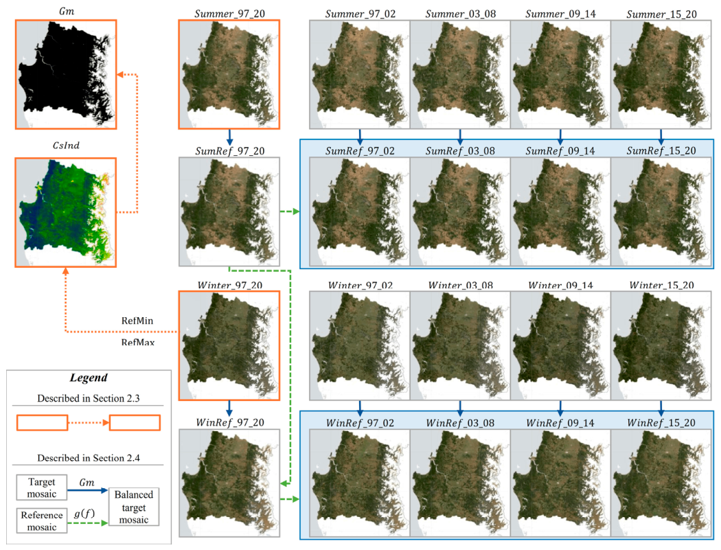
Two full-period mosaics, W i n t e r _ 97 _ 20 and S u m m e r _ 97 _ 20 , were created from scenes with less than 10% metadata cloudiness using median compositing; pixels represented by fewer than seven images were discarded. W i n t e r _ 97 _ 20 was used to calibrate one regional R e f M i n and R e f M a x value per sub-index. A single C s I n d threshold was then selected by visually comparing masked and unmasked versions of W i n t e r _ 97 _ 20 , prioritizing removal of cloud- or snow-contaminated pixels over retention of ambiguous pixels. The global mask ( G m ) was derived from C s I n d ( W i n t e r _ 97 _ 20 ) by removing values above the selected threshold and isolating low-coverage patches smaller than 2.7 ha. W i n t e r _ 97 _ 20 , S u m m e r _ 97 _ 20 , G m , and the calibrated C s I n d were retained for subsequent image and mosaic processing.

2.4. Radiometric Harmonization by Histogram Matching

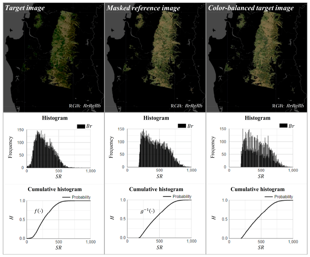
Per-band histogram matching, here termed color balancing, was used to reduce residual cross-sensor and cross-period radiometric differences [12,13,38,39,40]. This method defined transformation functions to map surface-reflectance values ( S R ) to cumulative histograms ( H ) and vice versa. For each target band B T a r , the forward function f is defined as H T a r = f ( S R T a r ) ; for a reference band B R e f , the backward function g is S R R e f = g ( H R e f ) . Both f and g were modeled as continuous, non-monotonic curves using RF regression—a secondary application distinct from the main RF described later. Applying f to the B T a r yields a cumulative-histogram band, B H T a r = f ( B T a r ) . The color-balanced target band is then obtained by applying g to align it with the reference histogram:
B T a r , R e f = g ( B H T a r ) = g ( f ( B T a r ) )
S u m m e r _ 97 _ 20 masked by G m formed the global summer reference, S u m R e f _ 97 _ 20 , whereas W i n t e r _ 97 _ 20 was first masked by G m and then balanced against S u m R e f _ 97 _ 20 to form the global winter reference, W i n R e f _ 97 _ 20 . The radiometric-reference mosaics were centered near 2011 rather than the 2009.3 midpoint.
Winter and summer mosaics were also produced for four six-year intervals: 1997–2002, 2003–2008, 2009–2014, and 2015–2020. They were balanced against the global radiometric references and served as partial references for shorter periods. Individual images were balanced only over pixels overlapping the appropriate partial reference, providing spatially adaptive matching. Hierarchical reference construction, local overlap matching, and RF-regression implementation are reported in Appendix A.1, Figure A1 and Figure A2.

2.5. Biennial Mosaics

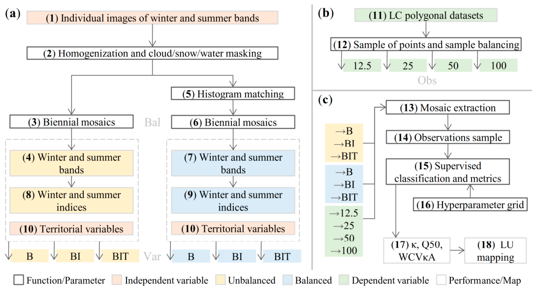
For each biennial period, winter and summer collections were filtered to less than 75% metadata cloudiness (Figure 2a, step 1). This threshold balanced spatial coverage and computation; higher thresholds added mostly unusable images. Each image was masked using the predefined quality masks, G m , and the corresponding C s I n d mask (step 2). Images with less than 5000 ha of unmasked area or average patch size were excluded because they did not support reliable histogram matching.

2.5.1. Color-Balancing Treatment Axis (Bal)

Color-unbalanced mosaics (“No” level) were produced as per-band medians without radiometric adjustment (steps 3–4). Color-balanced mosaics (“Yes” level) were generated by balancing each image against its partial reference before compositing, calculating the per-band median, and balancing the complete mosaic once more against the corresponding reference (steps 5–7).

2.5.2. Predictor-Set Treatment Axis (Var)

The winter and summer bands were supplemented with six seasonal indices and eight territorial variables (steps 8–10). The indices represented vegetation features ( E v i , G c i , and S i p i ) and LC-related features ( B s i , N b r i , and N d w i ). Territorial predictors represented terrain ( A s p e c t E , A s p e c t N , C h i l , and M t p i ), climate ( P r e p 06 , and T e m p 02 ), surface flow ( W b I n d ), and human accessibility ( A c c e s C i t y ). Definitions, equations, sources, and access links are reported in Table A2 and Table A3 (Appendix A.1).
Each predictor X was normalized to the 0–1 range according to: X n o r m a l i z e d = ( X m i n i m u m ( X ) ) / ( m a x i m u m ( X ) m i n i m u m ( X ) ) . For bands and indices, minimum and maximum values were calculated across periods to preserve temporal comparability; for invariant territorial variables, they were calculated by variable. This produced 12 biennial mosaics each containing 34 predictor layers (Table 2). Three nested predictor sets were used: B, seasonal bands; BI, B plus seasonal indices; and BIT, BI plus territorial variables.
Mean valid temporal coverage across the 12 mosaics was 85.5% and nearly complete in the core agroforestry area. Most missing data formed high-elevation fringes associated with persistent winter cloud or snow; fixed gaps also occurred over large water bodies and urban areas. Coastal limitations reflected the 1 km resolution of climatic predictors. Remaining gaps were addressed during post-classification processing in Section 2.9.

2.6. LC Reference Data and Observation Sampling

LC reference observations were extracted from Land-Use Change Monitoring polygons produced by the National Forest Corporation (CONAF) [41,42,43] (Figure 2b, step 11). Three nested legends served different purposes: C0 comprised 27 detailed LC classes used for classification; C1 pooled them into 12 classes for sample balancing; and C2 aggregated them into seven LU classes for transition analysis. Harmonization rules, category definitions, dataset links, and temporal references are in Table A5 and Table A6 (Appendix A.2).
Two temporal modes were used (step 12). In static mode, inventory dates matched the target period and all eligible polygons were retained. In dynamic mode, only polygons whose C0 class remained unchanged between the surrounding static inventories were used. P12 lacked reference data and was excluded from sampling and balancing, but it remained in the final LU reconstruction.
Random points were generated by period, with lower point density in large polygons and higher density in small polygons, and then merged into one dataset. Category and period frequencies were ranked to identify overrepresentation. No points were removed from the rarest category; category-based discard rates increased with frequency, and observations from overrepresented periods were removed above a predefined threshold. Appendix A.2 provides the point-generation, ranking, and discard rules.

Observation-Percentage Treatment Axis (Obs)

Four observation levels represented 12.5%, 25%, 50%, and 100% of the maximum available sample. Each level used a distinct random seed and was drawn from the full observation dataset before intersection with biennial mosaics to extract predictors and period identifiers (Figure 2c, 13). The computational limit was tested using large samples, the full predictor set, and extreme RF-hyperparameter values. Before percentage subsampling, seed-specific datasets averaged 10,922 points, with 140–2547 observations per C0 category and 245–1143 per period. Random subsets were then selected for each Obs level (step 14). Training and validation counts are reported in Table 3 (defined in Section 2.7).

2.7. RF Classification and Performance Metrics

The Obs, Bal, and Var axes generated 24 ungrouped treatments (Figure 2c, step 14). For each treatment, observations were divided into three parts: two for training and one for validation. Alternating the held-out part produced three sample variations.
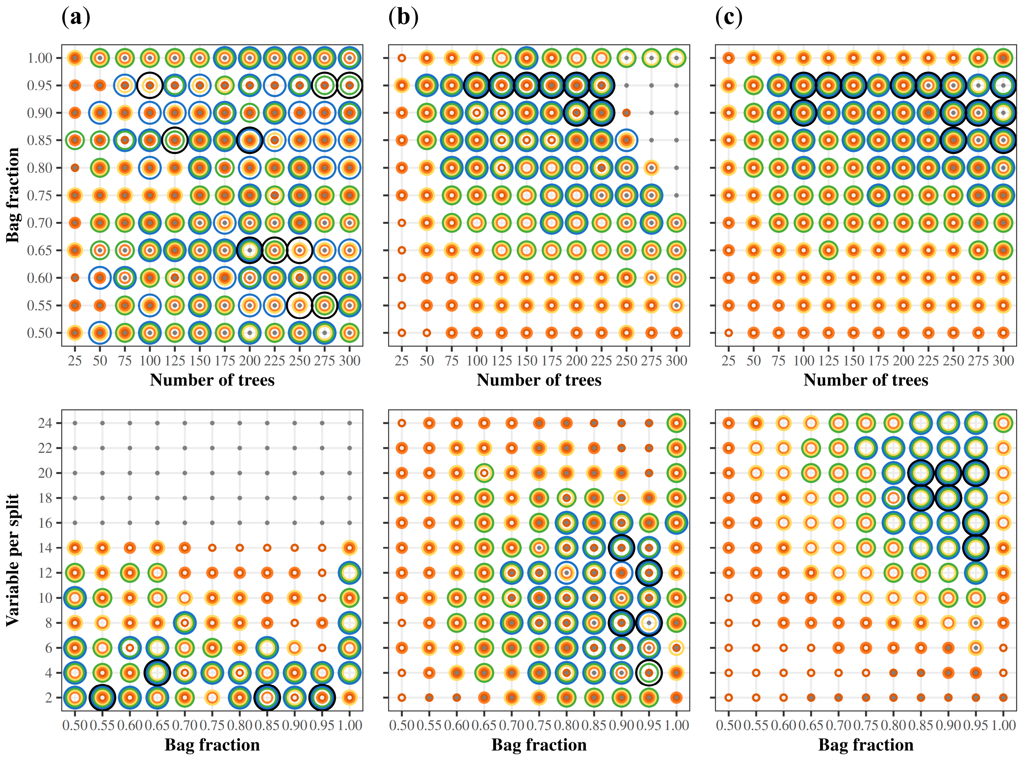
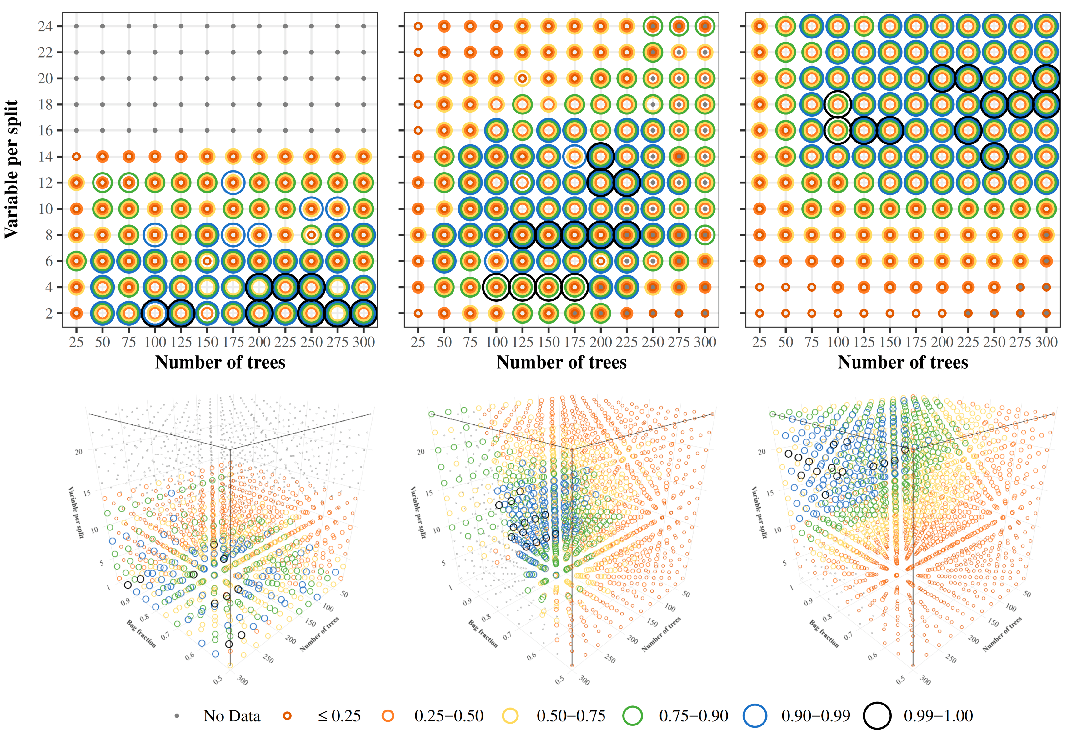
RF classification used ee-Classifier-smileRandomForest in GEE [44] and predicted the 27 C0 classes (step 15). RF hyperparameters were tuned using a grid search [45]. The grid evaluated bag fraction from 0.50 to 1.00 in 0.05 increments, number of trees from 25 to 300 in 25 increments, and variables per split from 2 to 24 in 2 increments (step 16). Minimum leaf population and maximum leaf nodes were unconstrained, allowing retention of rare classes. Across treatments, sample variations, and grid combinations, 31,944 classification measurements were obtained, with 757–1584 per ungrouped treatment.
Training and validation κ were averaged across the three sample variations (Figure 2c, step 17). For interpretation, κ was classified as poor (≤0.4), moderate (0.41–0.60), good (0.61–0.75), excellent (0.76–0.80), or almost perfect (>0.80) [46]. Training κ above 0.60 indicated low underfitting risk; a training–validation gap above 0.40 indicated high overfitting risk, whereas a gap below 0.15 indicated acceptable fit.
RF-hyperparameter dispersion was summarized using a custom metric, the weighted coefficient of variation by κ averaged (WCVκA):
W C V κ A = 1 / 3   · h 3 ( W S D κ h / W M N κ h )
For each hyperparameter ( h ), κ-weighted means and standard deviations ( W M N κ and W S D κ ) were calculated from configurations at or above the treatment-specific validation-κ median (Q50); the three resulting coefficients of variation were averaged.
Validation-κ Q50 and validation-WCVκA were analyzed jointly, representing median predictive performance and RF-hyperparameter dispersion among high-performing configurations. Low-, moderate-, and high-performance zones were defined using the existing Euclidean-distance equation based on each treatment’s deviation from the across-treatment means of both metrics. This criterion complemented context-dependent fixed κ thresholds and compared treatment accuracy and sensitivity to hyperparameter choice.

2.8. Treatment Comparisons, Selection, and Complementary Analyses

Normality, homoscedasticity, κ-comparison tests, paired κ differences, and effect-size procedures are detailed in Appendix A.3. Treatment evaluation proceeded from grouped to ungrouped analyses. Individual Obs, Bal, and Var axes and the combined Obs-Bal and Obs-Var groups were compared first. For ungrouped analyses, Obsi, Balj, and Vark denoted the respective axis levels. All ungrouped treatments, denoted Obsi-Balj-Vark, were then ranked by validation-κ Q50.
Ranking guided selection of contrasting Obs-No-BI and Obs-Yes-BIT series across Obs levels. They examined balancing and predictor-set effects, summarized RF-hyperparameter optima, and assessed training- and validation-κ stability. Hyperparameter statistics were calculated from classifications above the 99th percentile of validation κ. The highest three-fold validation-κ configuration per selected treatment was reevaluated in a new three-fold round, yielding six replications for standard deviation (SD) estimation.
Predictor importance was evaluated using RF mean decrease impurity [47,48]. Observation percentage and balancing state were fixed at their strongest levels, and the 100-Yes-Var series compared B, BI, and BIT. Mean decrease impurity values from six replications were averaged, ranked, and divided by the maximum within each predictor set.
The highest-ranked ungrouped treatment by validation-κ Q50 was selected for LU reconstruction.

2.9. LU Mapping and Change-Rate Analysis

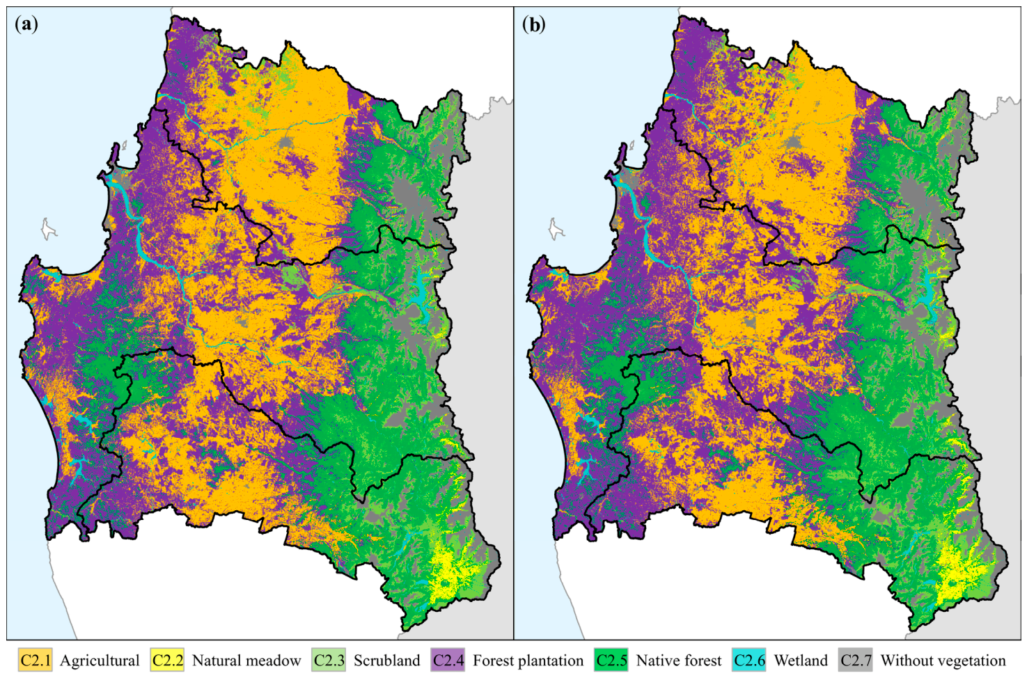
For the selected treatment, the model with the highest mean κ across the three sample variations was applied to all 12 biennial mosaics, producing three C0 classification series. For each period, the three maps were combined by pixel-wise statistical mode. Missing pixels were filled using adjacent-period classifications, index-based masks, and one-pixel local-mode extrapolation; Appendix A.4 provides the complete heuristics. Final maps were aggregated from C0 to C1 and C2 (Figure 2c, step 18).
Annual exponential LU-change rates (% year−1, base e) were compiled from studies overlapping the study area [5,6,30,32,49,50,51,52,53]. Literature-derived values were solved for r a t e using a two-point formulation, ln ( A r e a L a s t / A r e a F i r s t ) = ( r a t e / 100 ) · ( P e r i o d L a s t P e r i o d F i r s t ) ; whereas for this study were obtained across all periods using a continuous formulation, ln ( A r e a ) = ( r a t e / 100 ) · P e r i o d + c o n s t a n t . Published areas, calculations, and categories were harmonized or recalculated when required to match the C2 scheme.

2.10. Software

GEE (API REST v1) was used for image processing, random point sampling, RF classification, and post-classification analysis [3]; QGIS (version 3.38) was used to harmonize polygon datasets and prepare maps [54]; and R (version 4.3.1) was used for statistical analyses and performance graphics [55].

3. Results

3.1. Color-Unbalanced and Color-Balanced Biennial Mosaics

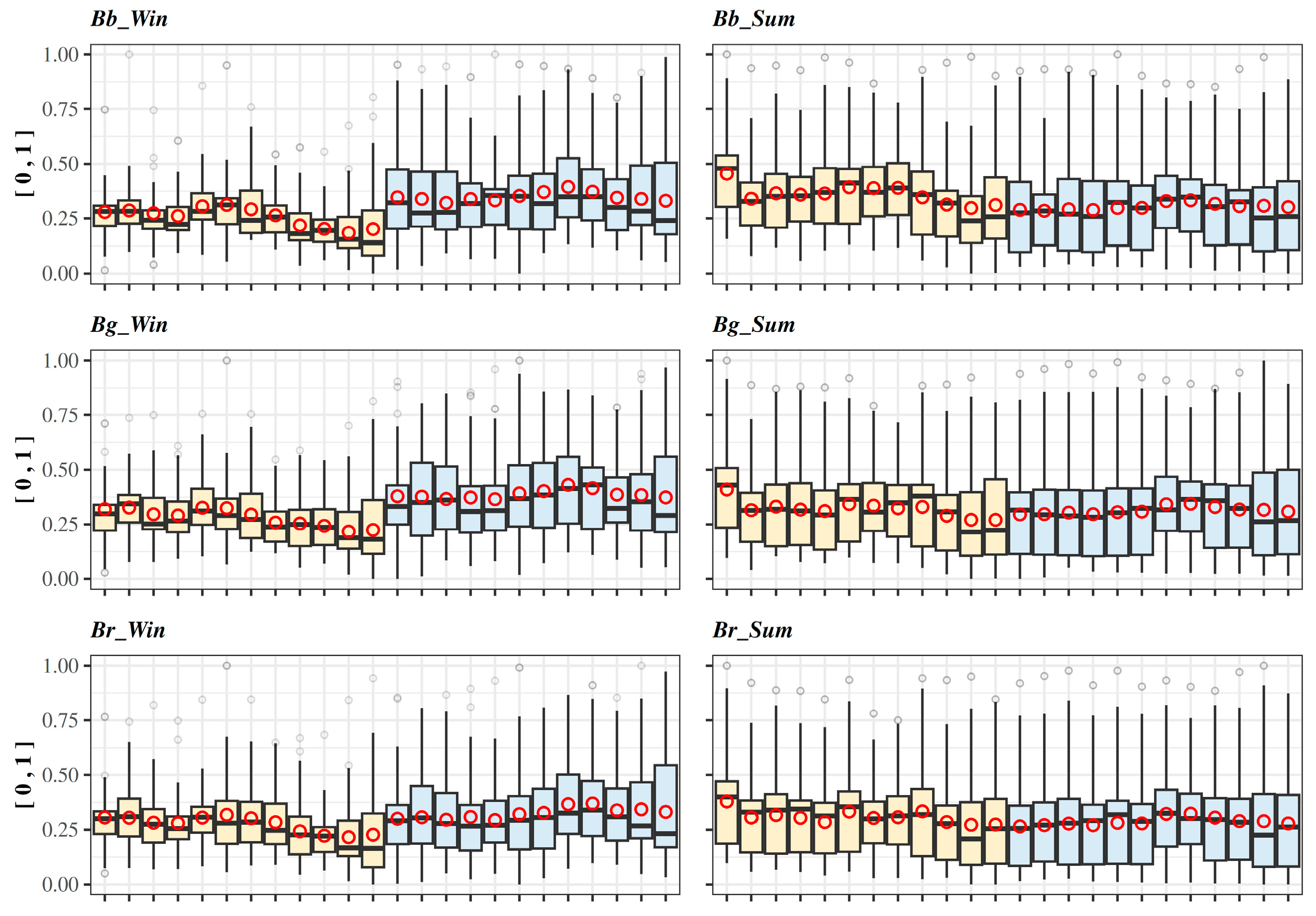
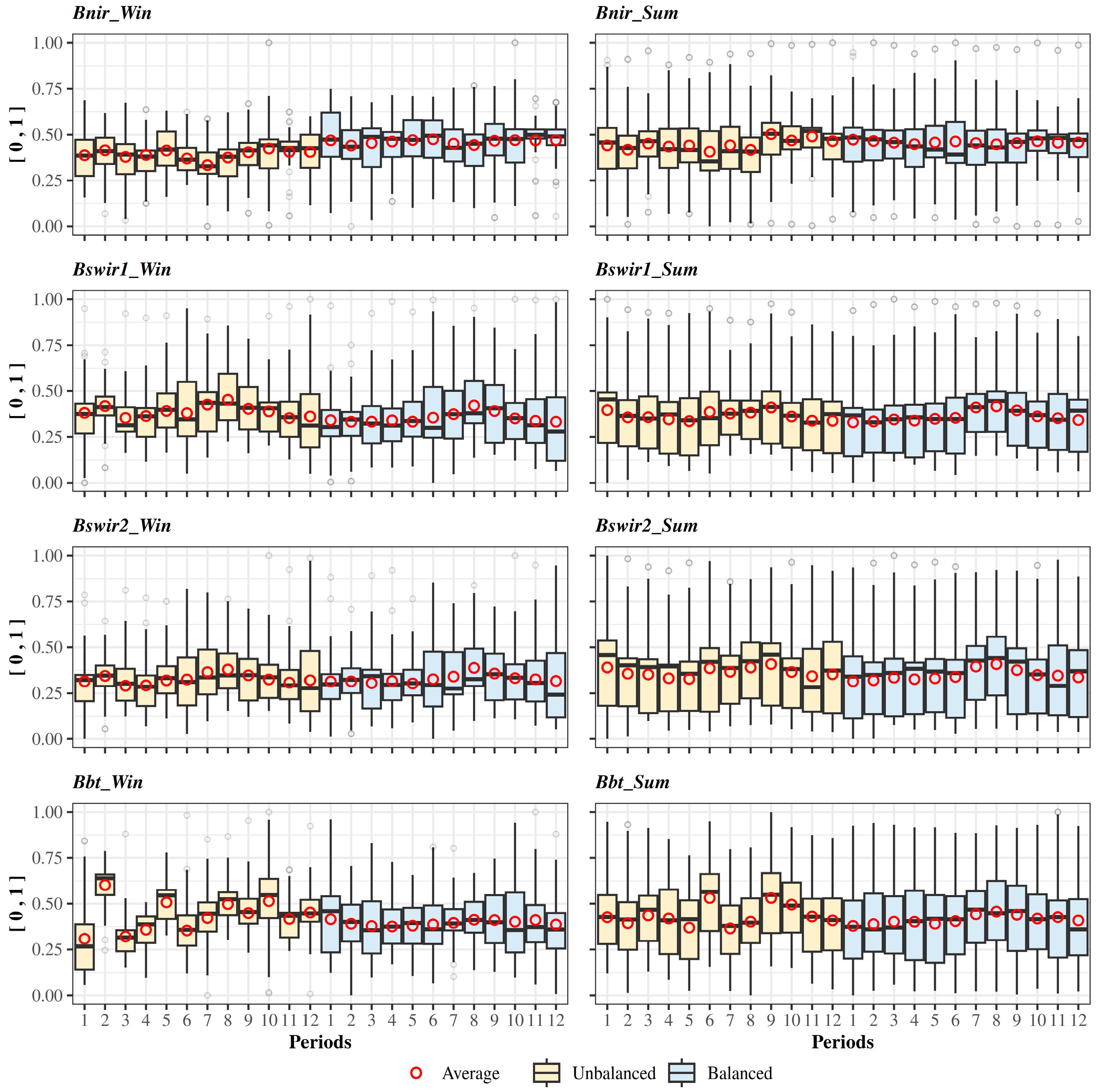
Color-unbalanced and color-balanced biennial mosaics were compared across periods and seasons to assess whether per-band histogram matching improved the consistency of spectral predictors before classification. The comparison used winter and summer Landsat composites generated under the balancing-axis treatments.
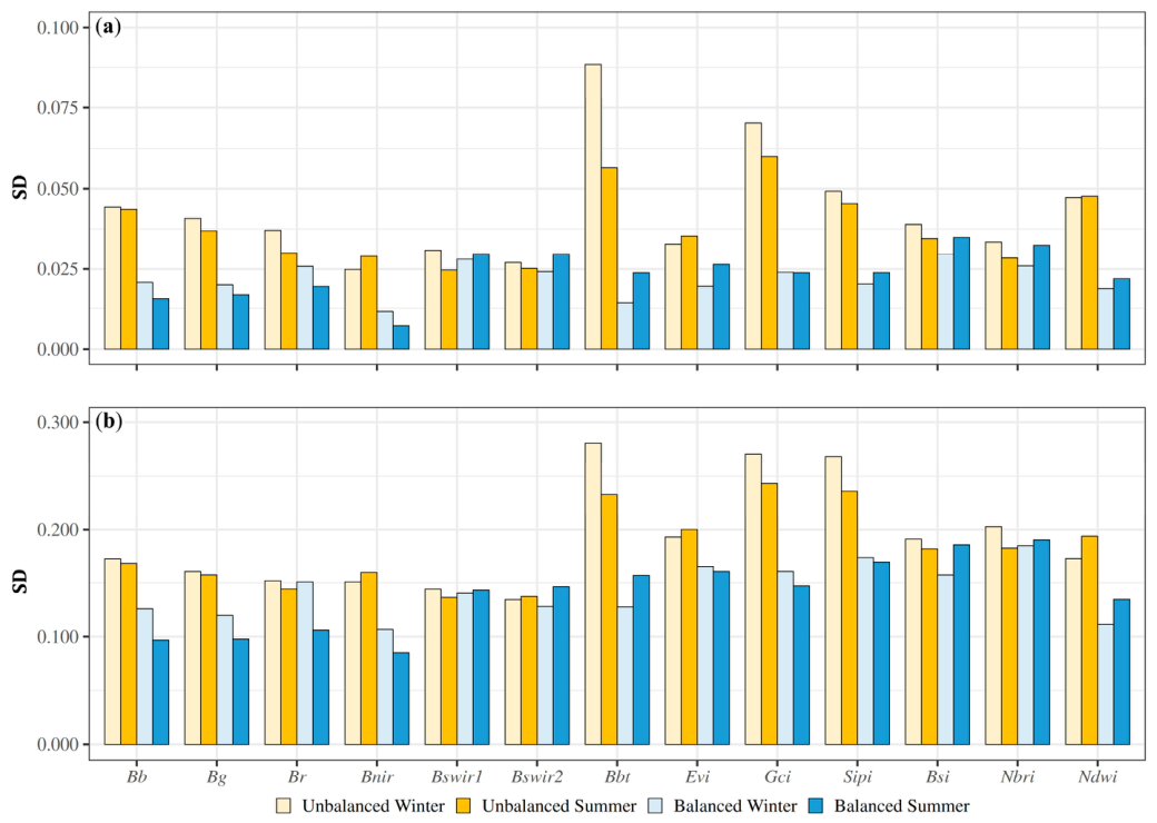
Figure 3 shows that summer variables had more stable distributions than winter variables in both central tendency and internal variability. Most spectral bands and indices also showed lower temporal dispersion after color balancing. Minor exceptions occurred for B s w i r 1 _ S u m , B s w i r 2 _ S u m , B s i _ S u m , and N b r i _ S u m , for which color-balanced values showed slightly higher variability. These exceptions were limited and did not alter the overall pattern of greater stability under summer conditions and after color balancing.
Period-level differences were also evident. P1 showed the greatest spectral misalignment, coinciding with low image availability and the inclusion of out-of-season imagery. P8 remained comparatively stable despite the dominance of L7 imagery affected by scan-line errors. Variability increased after P9, coinciding with the incorporation of L8 imagery and its different wavelength ranges and atmospheric-correction characteristics. Overall, residual spectral differences were period-specific and coincided with image availability, seasonal coverage, and sensor composition. These findings provide the empirical basis for the subsequent discussion of the effectiveness and limitations of color balancing.

3.2. Sample Distribution and Imbalance Across LC Categories and Periods

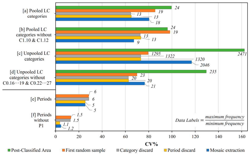
The post-classified area and observation-point distributions revealed substantial inherent imbalance across the landscape (Figure 4). Observation-point distributions remained imbalanced across LC categories and periods even after sampling and discarding. Each discarding rule also affected the opposite dimension: abundant categories were penalized most, wetlands remained unaffected, and native forests showed notable reductions. Period-based discarding reduced temporal overrepresentation, although data scarcity in P1 persisted.
Mosaic extraction affected categories unevenly and partially reintroduced category imbalance. C1.10-riverbank-and-shore and C1.12-without-vegetation showed the largest proportional reductions, mainly due to masking from snow, water, and adjacent pixels. C1.11-urban-and-industrial declined where high-reflectance urban surfaces overlapped spectrally with cloud–snow index responses. Natural meadows, scrubland, and native forests were also disproportionately reduced because of their concentration in mountainous terrain. The residual imbalance was concentrated mainly in rare or highly masked categories, including water-related (C0.16–C0.19), industrial-mining, and without-vegetation (C0.22–C0.27) classes. Overall, the sampling design controlled temporal imbalance more effectively than category imbalance.

3.3. Performance Zones Based on Validation-κ Q50 and WCVκA

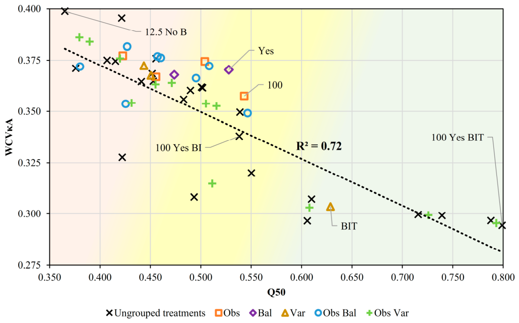
Validation-κ Q50 and validation-WCVκA were analyzed jointly to evaluate median classification performance and RF-hyperparameter dispersion among high-performing configurations. Figure 5 shows an inverse, roughly linear relationship among ungrouped treatments: as validation-κ Q50 increased, validation-WCVκA decreased. Thus, higher-performing treatments were associated with lower RF-hyperparameter dispersion. Grouped and combined grouped treatments followed the same trend, indicating consistency across analysis levels. Because training-κ values were consistently high, later comparisons focused on validation-related metrics and their variation across treatments.
Across grouped and combined grouped treatments, increasing the observation percentage or applying color balancing alone improved treatment position but was insufficient to reach the high-performance zone. The grouped 100%, color-balanced, and combined 100-Yes treatments reached only moderate performance. In contrast, the grouped BIT treatment produced the largest shift and entered the high-performance zone; among Obs-BIT combinations, only 12.5-BIT remained in the moderate zone.
Among ungrouped treatments, 100-Balj-B and 100-Balj-BI reached the moderate zone, but only their Yes versions did so consistently. Even 12.5-Balj-BIT treatments reached the moderate zone under both No and Yes conditions, while 25-, 50-, and 100-Balj-BIT treatments advanced progressively toward the high-performance zone. Validation-κ Q50 exceeded 0.75 for the 100-Balj-BIT treatments, indicating well-fitting configurations (Figure 5). This pattern extended the BIT advantage observed in the grouped analysis across balancing states and observation levels.

3.4. Validation-κ Across Grouped Treatments and Selected Ungrouped Series

Classification performance based on validation-κ differed clearly across treatment configurations, with predictor-set design producing the strongest overall contrast. Grouped treatments were first evaluated to identify the effects of each treatment axis. The complete ungrouped-treatment ranking was then used to select Obs-No-BI and Obs-Yes-BIT as contrasting series for assessing how color balancing and predictor-set design interacted across observation levels.
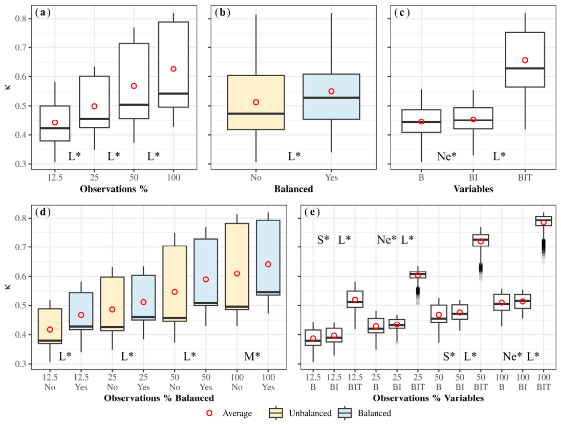
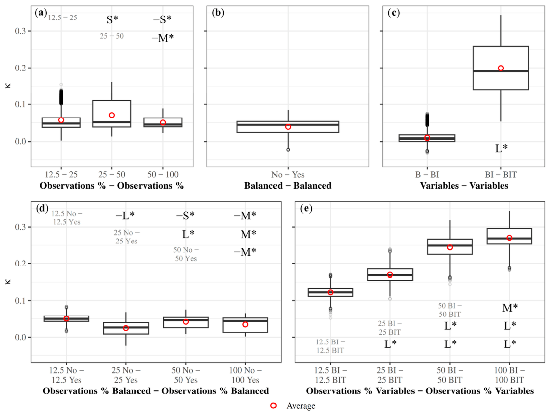
Increasing the observation percentage generally improved validation-κ (Figure 6a). However, paired κ differences alternated in sign between adjacent observation levels, indicating that the increase was weak and not consistently monotonic (Figure 7a).
Color balancing produced more symmetric distributions and reduced variability (Figure 6b). Paired κ differences confirmed a positive but modest effect relative to the predictor-set axis (Figure 7b,c). Combined Obs-Bal treatments showed a similar pattern, with generally lower dispersion after color balancing, particularly at lower observation levels (Figure 6d and Figure 7d).
Within the predictor-set axis, the transition from B to BI generated negligible κ changes, indicating that spectral indices added limited information beyond the original bands. In contrast, the transition from BI to BIT produced large improvements, representing the strongest gain among the single-axis analyses (Figure 6c and Figure 7c). Obs-Var combinations reinforced this pattern: differences remained limited from Obs-B to Obs-BI but were consistently positive from Obs-BI to Obs-BIT (Figure 6e and Figure 7e). These differences remained positive across all observation levels, although their magnitude decreased at higher levels.
The complete ranking of ungrouped treatments followed the same overall trends identified in the grouped analyses and revealed no additional major patterns. One minor pattern was that Obsi-Balj-BI treatments generally showed lower validation-κ dispersion than their Obsi-Balj-B counterparts, although this did not consistently translate into higher performance. Detailed results are provided in Appendix B.2.
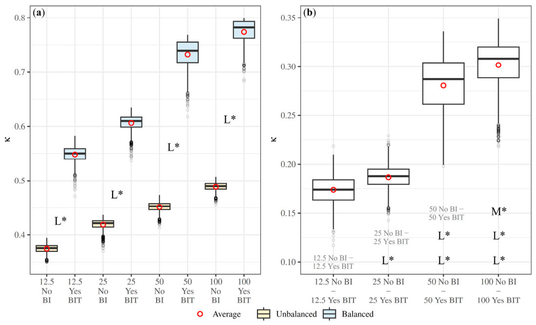
Within the contrasting Obs-No-BI and Obs-Yes-BIT series, performance followed a consistent ranking from 12.5-No-BI to 100-Yes-BIT (Figure 8). At each observation level, Obsi-Yes-BIT outperformed the corresponding Obsi-No-BI treatment. The Obsi-No-BI series increased gradually, whereas Obsi-Yes-BIT showed a stronger shift after the 25% level, widening the separation between the two series.
Overall, the grouped and selected ungrouped analyses consistently identified predictor-set design as the principal source of performance differences, while observation percentage and color balancing produced smaller and less uniform effects.

3.5. Predictor Importance

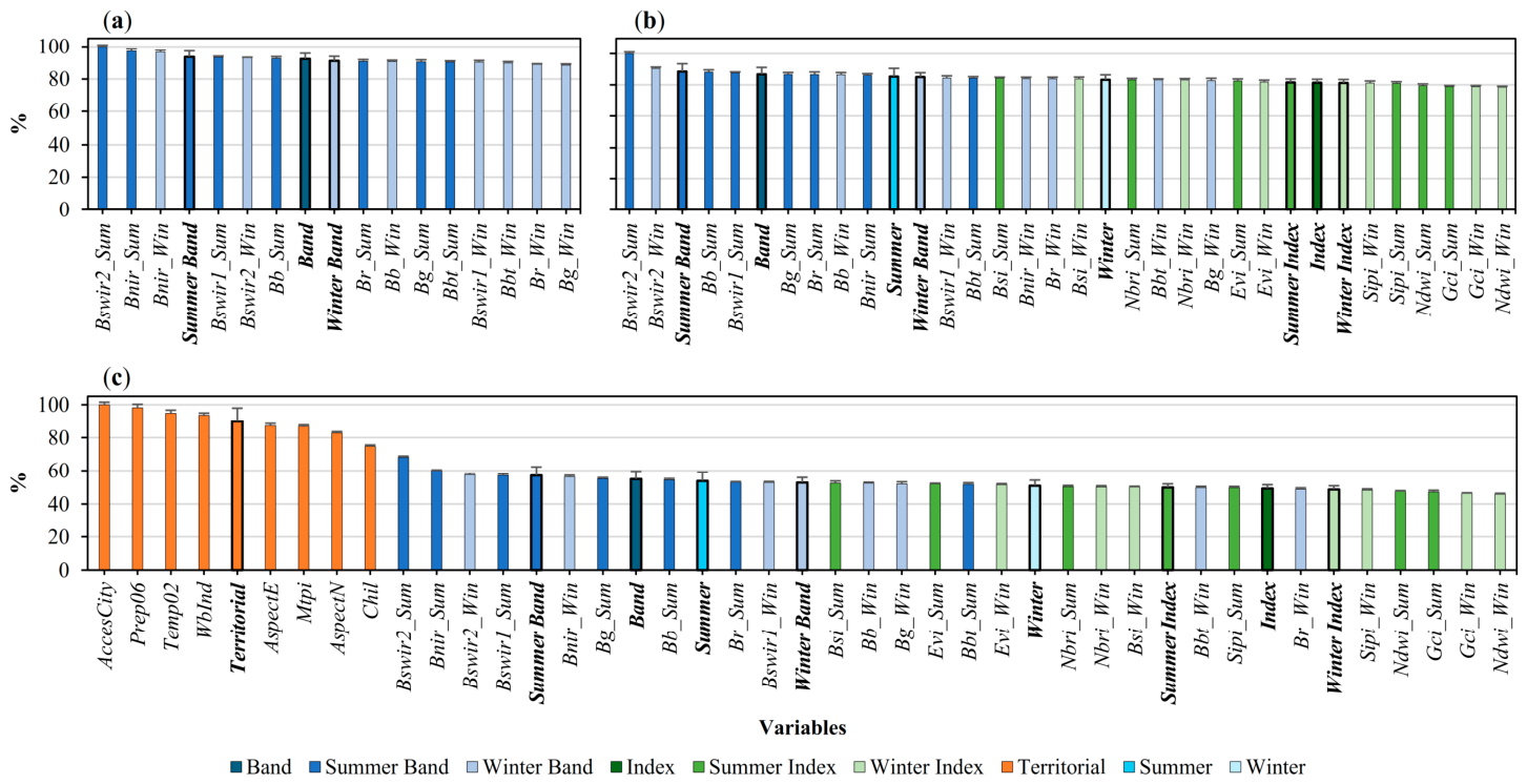
Based on the treatment comparisons, the best-performing levels within the Obs and Bal axes, 100% observations and color balancing, were held constant to compare predictor importance across the B, BI, and BIT predictor sets. Figure 9 shows a clear hierarchy in the full predictor set: territorial variables generally ranked highest, followed by spectral bands, whereas spectral indices ranked lowest. Spectral-predictor rankings were otherwise broadly consistent across the 100-Yes-B, 100-Yes-BI, and 100-Yes-BIT treatments.
Among spectral predictors, summer variables generally ranked above their winter counterparts. B s w i r 2 _ S u m and B s w i r 2 _ W i n ranked highest, followed by B n i r _ S u m and B n i r _ W i n , although these predictors shifted toward intermediate positions in 100-Yes-BI. B s w i r 1 _ S u m ranked comparably to other summer bands, whereas B s w i r 1 _ W i n shifted toward the lower range. Visible bands occupied intermediate positions, except B r _ W i n and B g _ W i n , which ranked among the lowest together with the thermal bands. Among spectral indices, E v i , B s i , and N b r i showed moderate importance, whereas G c i , S i p i , and N d w i consistently ranked lowest. Among territorial variables, accessibility to cities and water bodies and climatic factors occupied several of the highest-ranking positions, followed by terrain metrics. Overall, the predictor-importance results reproduced the performance hierarchy observed among the B, BI, and BIT treatments.

3.6. RF Hyperparameters

RF-hyperparameter distributions differed between the Obs-No-BI and Obs-Yes-BIT series, although the contrast varied among parameters (Table 4). Bag fraction and number of trees showed limited or inconsistent series-level patterns, whereas variables per split produced the clearest between-series differences.
For bag fraction, 12.5-No-BI showed the broadest range, followed by 25-No-BI, whereas the remaining treatments had similar Q50 and Opt values. High bag-fraction values were common among high-performing configurations but did not vary systematically with performance.
For number of trees, Q50 values ranged from 163 to 250, and maximum values reached 300 in most treatments. Opt values ranged from 100 to 300 but did not increase systematically with performance. Moreover, 100-Yes-BIT showed the highest number-of-trees dispersion despite being the best-performing treatment. Thus, number of trees showed no consistent series-level pattern.
Variables per split showed the clearest contrast between the two series in both dispersion and central values. In Obs-No-BI, CV was consistently higher and generally declined as observation percentage increased, while Q50 and Opt values decreased markedly from 12.5–25% to 50–100%. In contrast, Obs-Yes-BIT showed lower overall dispersion, with Q50 and Opt values increasing from 12.5–25% to 50–100%.
Overall, variables per split distinguished the two treatment series more clearly than bag fraction or number of trees.

3.7. Land-Use Areas and Transitions

Based on the ungrouped-treatment ranking, 100-Yes-BIT was identified as the highest-performing treatment and selected for LU reconstruction. Its optimal configuration– bag fraction = 0.90, number of trees = 250, and variables per split = 18 (Table 4)– achieved κ = 0.820 for Code 0 and κ = 0.910 for Code 2. Additional performance values for the contrasting series are reported in Table A15 (Appendix B.2); for example, 100-No-BI achieved κ = 0.507–0.743 as the pooling code increased.
Two complementary criteria were used to examine LU areas: first-to-last changes between P1 and P12 and all-period transitions across P1–P12. Table 5 shows that forest plantations and agricultural land jointly dominate the landscape, accounting for approximately 60% of the study area. Native forest and scrubland together accounted for approximately 28%, confirming the mixed agroforestry character of the region. Differences between temporal averages were generally small.
Regarding change rates and temporal consistency, agriculture and wetlands showed the strongest declines and a high R2 value of approximately 0.90, indicating consistent downward trajectories. Forest plantations showed a relatively consistent expansion (R2 = 0.77), while without-vegetation areas showed a smaller but similar regular increase. Natural meadows and scrubland had weaker consistency (R2 ≈ 0.4) although opposite directions of change; whereas native forest combined little rate with the lowest R2, reflecting irregular inter-period dynamics.
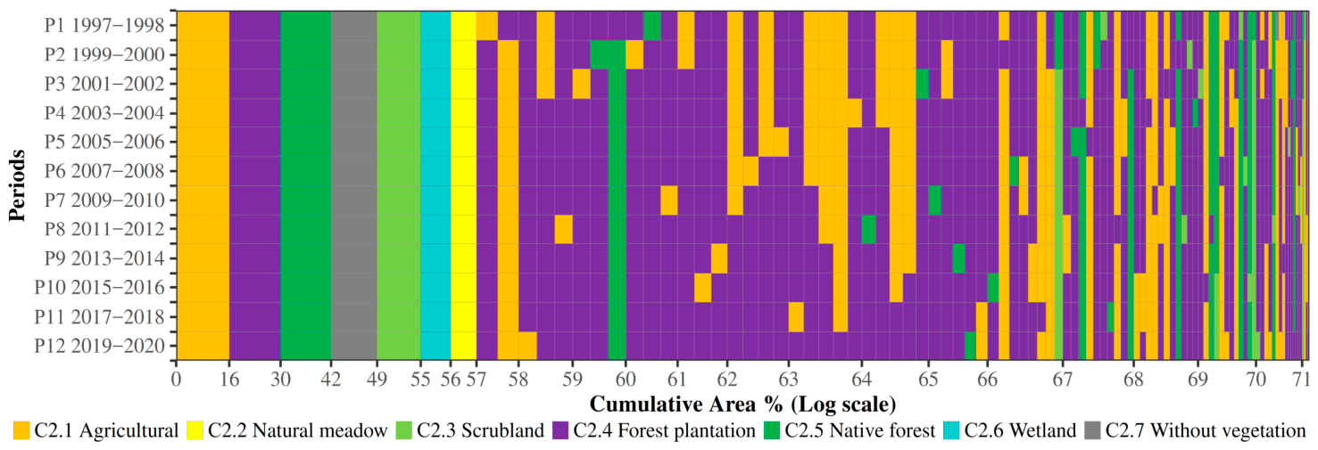
Categories remaining unchanged throughout P1–P12 accounted for 57.1% of the study area (Figure 10). The 22% difference between unchanged areas under the two criteria indicates substantial intermediate dynamics not captured by first-to-last comparisons. Intermediate dynamics were concentrated mainly in forest plantations and agricultural land, producing differences in losses, gains, net change, and annual rates. All-period estimates showed faster declines in agriculture and wetlands and faster forest-plantation expansion than first-to-last estimates (Table 5). Spatially, the dominant transition was from agricultural land to forest plantations, mainly within established forestry zones of the Coastal Range and Central Depression and, to a lesser extent, into native-forest patches along the Coastal Range. Among smaller categories, natural meadows expanded mainly over degraded scrubland and native forest, whereas wetlands declined through conversion to agriculture and forest plantations.
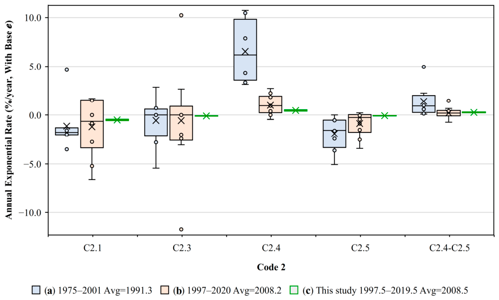
To compare the estimated LU-change rates with literature-derived values, Figure 11 summarizes annual exponential rates for the LU categories with the greatest data availability. The compiled rates were grouped into an earlier period, 1975–2001, and a more recent period, 1997–2020, and compared with the first-to-last and all-period estimates from this study.
Agricultural rates were predominantly negative across the literature, and the estimates from this study (−0.43 and −0.57) were similar to those reported for comparable spatial extents (−0.83 to −0.54 [51,52,53]). Forest-plantation rates were predominantly positive but generally lower in the recent literature group. The estimates from this study (0.39 and 0.52) were comparable to similar-area values of 0.30–0.38 [5,51], although a higher value of 0.95 was also reported [52]. Native-forest rates remained negative but approached zero in the recent group, consistent with the estimates from this study (−0.10 and −0.07) and regional values of −0.06 to −0.05 [5]. When native forests and forest plantations were pooled, the estimates from this study (0.21 and 0.31) were also consistent with the recent-group average and regional values of 0.21–0.38 [5,52].
Other categories showed less consistent evidence. Scrubland rates remained generally close to zero without a clear direction, while values for natural meadows and without-vegetation areas were scarce and variable. Wetland rates also varied substantially, although the estimates from this study (−0.62 and −0.74) closely matched the value reported for the same spatial extent (−0.60 [51]).
Overall, the reconstructed series and literature-derived comparisons identified agricultural decline and forest-plantation expansion as the clearest regional patterns, while smaller categories showed more variable trajectories.

4. Discussion

4.1. Data Quality, Harmonization, and Sample Imbalance

Integrating imagery from multiple satellites and territorial zones extends coverage but requires homogenization to limit sensor-, season-, and period-related artifacts [56,57]. Histogram matching did not fully correct spectral differences, but it reduced mismatches that could otherwise be interpreted as LC/LU change. Stable distributions despite L7 scan-line errors also supported the compositing and smoothing strategy. The limited response of B s w i r 1 and B s w i r 2 suggests that these bands were stable before harmonization, while the remaining exceptions show that improvements were not uniform. Shortwave-infrared and thermal predictors are relatively resistant to atmospheric scattering and capture vegetation structure, moisture, and surface-temperature gradients [58], which may improve discrimination of spectrally ambiguous categories. The procedure nevertheless assumes that bands can be harmonized independently. Future refinements could account for inter-band correlations using multidimensional histograms or color-space transformations [14]. Reliance on a master reference image is another limitation, while direct image-fusion methods remain difficult to adapt to multispectral data [59]. Color balancing should therefore be treated as a harmonization aid, not a universal correction.
Sample imbalance poses a related problem because equal representation cannot usually be achieved without information loss. Downsampling to the rarest class discards useful observations, whereas oversampling adds no information and may create artificial spatial dependence. Slightly imbalanced samples can outperform perfectly balanced ones [16,17], and studies have mainly addressed class imbalance rather than temporal or territorial imbalance [7,16,17]. Although category-based CVs were high, the pooled maximum-to-minimum ratio (18) was close to Zhu et al. [17] (13), and the unpooled ratio (2026) fell within the 1101–15,922 range reported by Hermosilla et al. [7]. Thus, residual imbalance was comparable to previous studies and was a practical rather than exceptional constraint. It nevertheless increased uncertainty for rare, masked, or spectrally ambiguous categories. Leaving min-leaf-population unconstrained allowed individual observations to define leaf nodes and preserved rare-class signatures, although at greater overfitting risk.
Its independent effect on accuracy could not be isolated, but RF remains suitable because of its tolerance to imbalanced and noisy training data [16,20,60,61,62]. Overall, radiometric harmonization reduced spectral inconsistencies, while controlled imbalance preserved rare-category information. These measures mitigate different input-data biases without eliminating uncertainty.

4.2. Treatment Effects and Predictor Design

Increasing the number of observations generally improved performance by providing broader class representation, but gains diminished at higher levels, suggesting an emerging saturation pattern rather than a precise sample threshold. Some computationally demanding classifications were unavailable because of GEE limits, although the small gains at the upper observation levels suggest that this missingness did not materially alter the general pattern. Future studies should test finer sample increments using less restrictive computing environments.
Color balancing addressed a different constraint by improving temporal spectral consistency rather than adding class information. Its declining marginal contribution as sample size increased suggests a partial trade-off between radiometric harmonization and observation availability. It may therefore be most valuable when reference data are limited or further sampling is impractical, while remaining complementary to predictor design rather than replacing informative variables.
The limited improvement from adding spectral indices is mainly due to redundancy. Because the seasonal indices are algebraic transformations of the same winter and summer bands already included in the baseline predictor set, they emphasize spectral relationships but add limited independent information. Moreover, the two seasonal band sets already expose RF to winter–summer differences, while RF can capture nonlinear relationships and interactions directly from the original bands and tolerate multicollinearity [20,21,63,64]. Thus, the ecological interpretability of indices does not necessarily translate into additional predictive information. Bera et al. [18] likewise found no consistent hierarchy between bands and indices, indicating that their value is context-dependent. The low importance of G c i , S i p i , and N d w i likely reflects information already represented by B n i r and the visible band. However, as predictor sets were cumulative, comparisons with indices-only configurations are needed to isolate their independent contribution.
In contrast, territorial variables produced stronger gains because they introduced nonredundant spatial context not derivable directly from the seasonal spectral bands. Previous work has similarly shown that elevation, slope, and proximity to water can equal or exceed spectral predictors [7]. Although Level-2 surface-reflectance products correct major physical effects [33,34,35], they do not encode landscape position, accessibility, or environmental gradients associated with LC/LU patterns. Variables such as W b I n d and A c c e s C i t y therefore helped distinguish spectrally similar categories, including wetlands with variable vegetation and natural versus artificial bare soil.
These contextual gradients were also consistent with established LU distributions, including agriculture on gentle, irrigated terrain, forestry on steeper slopes near roads, and native forest in higher, rugged areas [6,28,65]. These associations are explanatory rather than causal, and predictor rankings based on mean decrease impurity remain sensitive to RF stochasticity, tree number, and calibration [22,66]. Nevertheless, the results imply that informative predictor design can partly compensate for limited samples, whereas additional observations and color balancing provide complementary but smaller benefits.

4.3. Performance Zones and RF-Hyperparameter Tuning

Performance zones complemented fixed κ thresholds by combining median validation performance with RF-hyperparameter dispersion. Although κ remains useful for multi-class and imbalanced classification because it adjusts agreement for chance [45], fixed thresholds are context-dependent [45,67]. RF fit also reflects model complexity, noise, irrelevant predictors, and the bias–variance trade-off, while its ability to prevent overfitting remains debated [16,20,45,64,68,69]. Low variability across cross-validation replications further suggests that treatment configuration, rather than random sample splits, drove the main performance differences.
To place these results in broader quantitative context, Sun and Ongsomwang [23], using Sentinel-2 spectral and auxiliary data with RF, obtained κ = 0.91 (6 classes), consistent with the optimal 100-Yes-BIT configuration here (κ = 0.82–0.91; 27–7 classes). Nguyen et al. [70] compared parametric multinomial logistic regression with conventional machine-learning classifiers (k-nearest neighbors, support vector machine, and RF) using multi-season Sentinel-2 bands and obtained κ = 0.61–0.81 (11 classes). Sentinel-2 deep-learning approaches achieved κ = 0.71–0.76 (23–7 classes) with Swin-UNet [71] and κ = 0.87 (8 classes) with a multi-year IRUNet ensemble [72]. These values slightly exceeded the optimal spectral-only 100-No-BI configuration here (κ = 0.51–0.74; 27–7 classes).
Beyond numerical performance, these models illustrate an interpretability–flexibility continuum rather than a hierarchy. Parametric models offer direct parameter-level interpretation but impose stronger functional assumptions, whereas deep-learning architectures provide greater flexibility but rely on latent features less directly linked to physical predictors. Conventional machine-learning approaches such as RF occupy an intermediate position, capturing nonlinear interactions while retaining partial interpretability through predictor-set comparisons and variable importance [64]. Because study designs differ, these κ values are contextual benchmarks rather than direct model rankings.
Within this study, however, interpretation of WCVκA remains exploratory because it depends on its weighting scheme and on κ values above Q50. Alternative weighting and scaling approaches should therefore be tested. Nevertheless, the inverse relationship supports jointly using validation-κ Q50 and validation-WCVκA to select treatments based on median performance and convergence, rather than on a single optimal configuration.
The tuning results translate this convergence pattern into parameter-specific recommendations. Bag fraction was highly data-dependent, consistent with reported optimal ranges of 0.1–0.9 [18,23,44,73], and therefore requires at least coarse tuning. A value of 1.0 may be suboptimal because it removes bagging stochasticity. Number of trees showed similarly broad behavior. Studies have tested 10–5000 trees and commonly reported optima of 150–1000 [18,20,23,73], while Svoboda et al. [73] identified 150 trees as optimal after testing up to 400. Increasing ensemble size may promote stabilization, but the maximum tested value should not be assumed optimal.
The variables-per-split parameter was more sensitive to predictor composition. Common starting rules include the square root, one-third, or all predictors [18,20,44,74,75], with the one-third rule supported here as a practical baseline rather than a universal optimum. However, the two series showed opposite trends as observation percentage increased. In Obs-No-BI, variables per split decreased, possibly because smaller predictor subsets reduced redundancy among indices that largely recombined spectral-band information. In contrast, variables per split increased in Obs-Yes-BIT, potentially allowing the model to exploit the nonredundant context provided by territorial variables. This parameter should therefore be calibrated according to both predictor composition and observation availability, whereas bag fraction and number of trees may be tuned more coarsely.

4.4. Reliability and Comparability of LU Change

The LU patterns should be interpreted through classification uncertainty and temporal consistency. Agriculture and forest-plantation changes are better supported by broad spatial representation and clear regional patterns. Wetlands, natural meadows, scrubland, and small native-forest patches are sensitive to spectral confusion, limited representation, and temporal inconsistency. Sample imbalance and spectral confusion may interact because fewer observations reduce representation of within-class variability, while spectral overlap with more abundant classes can increase omission and commission errors. When independently classified periods are compared, these errors may propagate into apparent gains or losses, particularly for small categories. Their estimates are therefore more reliable for indicating direction and relative magnitude than exact pixel-level conversions.
These category-level limitations also constrain cross-study comparison despite harmonization and recalculation. Previous studies merged wetlands with agriculture or scrubland [6,30], natural meadows with agriculture and scrubland [5,50,53], and scrubland with native forest [6,32]. These differences may reflect grazing on degraded land, weak separation of managed and natural grasslands, and inconsistent scrubland definitions. Small categories were also frequently omitted or merged. Literature-derived rates should therefore be treated as contextual references rather than direct validation.
Within these constraints, reliability depended on agreement between internal temporal consistency and external evidence. Agriculture and forest plantations provided the strongest support because their trajectories were consistent and broadly agreed with studies covering comparable areas. Wetland decline was internally consistent, but small extent, spectral ambiguity, limited literature, and frequent category merging reduced broader confidence. Native forest showed a generally declining direction consistent with regional studies, although irregular inter-period dynamics weakened support for a continuous trend. Scrubland, natural meadows, and without-vegetation areas showed more variable trajectories and weaker comparative evidence. Some were also concentrated in mountainous areas with limited imagery, where residual gaps required heuristic post-classification filling. Thus, dominant and consistently defined categories support more reliable change directions than small, ambiguous, or inconsistently classified ones.
Beyond category-level limitations, the generally lower estimated rates may partly reflect the classification design. Persistent areas dominated the landscape so that sampling may have represented persistence more strongly than change. In addition, invariant territorial predictors emphasized stable spatial contrasts rather than temporal dynamics. Together, these mechanisms may have favored persistent classifications and reduced estimated change magnitudes. Future work should balance observations by change versus persistence and, where feasible, transition type, in addition to category and period. Transition-based approaches such as Land-Use 2.0 could classify transitions and persistence directly rather than infer them from independently classified periods [15], strengthening change estimates.
A further limitation is that spatial transition uncertainty was not quantified. The final LU reconstruction used the modal class of three classification series generated from the three sample variations of the single optimal RF-hyperparameter configuration in 100-Yes-BIT. Variation among these series therefore reflects sensitivity to the three-fold sample variation for that configuration, rather than variability across the high-performing RF-hyperparameter configurations evaluated for the treatment. A broader uncertainty assessment should consider both sources of variation before deriving spatial, category-level, or transition-level uncertainty for LU transitions.

5. Conclusions

This study provides four conclusions and practical recommendations for multi-decadal LC/LU mapping under limited spatial and temporal data.
First, mapping reliability depended more on observation quality, seasonal coverage, and temporal representativeness than on archive size, while radiometric harmonization improved cross-sensor and cross-period consistency. Multi-temporal workflows should therefore prioritize high-quality, seasonally consistent imagery and explicit harmonization rather than maximizing image quantity.
Second, perfect sample balance was neither feasible nor desirable because it would discard information from dominant classes or artificially replicate rare ones. However, retaining very small samples increased uncertainty and overfitting risk. Sampling designs should seek controlled balance and explicitly report uncertainty for rare, masked, and spectrally ambiguous categories.
Third, predictor design was the main determinant of performance: spectral indices contributed limited new information, color balancing improved temporal consistency, and territorial variables added nonredundant environmental and spatial context that improved class discrimination. Data-limited applications should therefore prioritize relevant territorial predictors, using color balancing and additional observations as complementary measures rather than substitutes for informative predictor design.
Fourth, model selection should jointly consider validation accuracy and RF-hyperparameter dispersion because high-performing treatments showed greater convergence across plausible configurations, whereas weaker treatments depended more strongly on specific settings. Treatments should therefore be selected using high median accuracy and low dispersion, with coarse tuning for bag fraction and tree number and predictor-dependent calibration of variables per split.
The reconstructed LU series supported the regional importance of agricultural decline and forest-plantation expansion, but transition reliability was higher for dominant, consistently classified categories than for small or spectrally ambiguous ones. Transition-specific spatial uncertainty was not quantified; future work should consider both three-fold sample variation and variability among high-performing RF-hyperparameter configurations. Literature-derived rates should be treated as contextual comparisons rather than direct validation, and future studies should balance observations by change versus persistence and, where feasible, by transition type.

Author Contributions

Conceptualization, methodology, resources, project administration, and funding acquisition, M.A. and L.V.O.; software, validation, formal analysis, investigation, data curation, writing—original draft preparation, and visualization, L.V.O.; writing—review and editing, and supervision, M.A. All authors have read and agreed to the published version of the manuscript.

Funding

This research was funded by the National Agency for Research and Development (ANID) National Doctorate Scholarship 2018, grant number 21181447, and by ANID National Fund for Scientific and Technological Development (FONDECYT), grant number 1231382.

Data Availability Statement

The data supporting the findings of this study are contained within the article. Additional LC/LU data products may be made available upon reasonable request.

Acknowledgments

The authors acknowledge the Environmental Remote-Sensing Laboratory, EULA-Chile Centre, University of Concepción, for providing materials and a supportive working environment.

Conflicts of Interest

The authors declare no conflicts of interest. The funders had no role in the design of the study; in the collection, analyses, or interpretation of data; in the writing of the manuscript; or in the decision to publish the results.

Abbreviations

The following abbreviations, codes, symbols, and mathematical notations are used in this manuscript:
A c c e s C i t y Accessibility to cities
ANID National Agency for Research and Development of Chile
A s p e c t E East-aspect component
A s p e c t N North-aspect component
Avg Average
B Predictor-set level containing seasonal spectral bands
Bal|Balj Color-balancing axis|jth Bal level
B b Blue band
B b t Brightness-temperature band
B g Green band
BI Predictor-set level containing B + spectral indices
BIT Predictor-set level containing BI + territorial variables
B n i r Near-infrared band
B r Red band
B R e f Reference band
B s i Bare soil index
B s w i r 1 Shortwave-infrared band 1
B s w i r 2 Shortwave-infrared band 2
B T a r Target band
B T a r , R e f Target band color-balanced to the reference
B H Cumulative-histogram band
C0.1–C0.27 Unpooled land-cover category codes
C1.1–C1.12 Pooled land-cover category codes
C2.1–C2.7 Pooled land-use category codes
C h i l Continuous heat-insolation load index
CI Confidence interval
CONAF National Forest Corporation of Chile
C s I n d Cloud–snow index
CV Coefficient of variation (%)
DOY Day of year
E v i Enhanced vegetation index
f Forward cumulative-histogram function
FONDECYT National Fund for Scientific and Technological Development of Chile
g Backward cumulative-histogram function
G c i Green chlorophyll index
GEE Google Earth Engine
G m Global mask
H Cumulative histogram
L Large effect size
L5, L7, L8 Landsat 5, 7, 8
LC Land cover
LU Land use
M Moderate effect size
Max Maximum
Max.SD Maximum of compared standard deviations
Min Minimum
Min.SD Minimum of compared standard deviations
M t p i Multi-scale topographic position index
Number of cases included in the corresponding analysis
N b r i Normalized burned ratio index
N d w i Normalized difference water index
Ne Negligible effect size
N.Max Theoretical maximum number of measurements
N % Non-missing measurements (%)
No Color-unbalanced Bal level
Obs | Obsi Observation-percentage axis | ith Obs level
Opt Optimal value achieving maximum performance
P1–P12 Biennial period codes
P r e p 06 June precipitation
Q50 50th percentile (median)
Q 50 Median of paired differences
QGIS Geographic information system software
R Statistical computing environment
R2 Coefficient of determination
R e f M a x Local reference maximum
R e f M i n Local reference minimum
RF Random Forest
RGB Red–green–blue display
S Small effect size
SD Standard deviation
S i p i Structure-insensitive pigment index
SR   ( S R ) Surface reflectance
S u m Summer mosaic
S u m R e f Summer radiometric-reference mosaic
T1–T7 Temporal reference codes for LC polygon datasets
T e m p 02 February temperature
Var | Vark Predictor-set axis | kth Var level
W b I n d Water-body index
WCV κ A   ( W C V κ A ) Weighted coefficient of variation by kappa averaged
W i n Winter mosaic
W i n R e f Winter radiometric-reference mosaic
W M N κ κ-weighted mean
W S D κ κ-weighted standard deviation
Q 50 Difference between two Q50 values
κ Cohen’s kappa agreement statistic
Yes Color-balanced Bal level
* Statistical significance (probability < 0.001)

Appendix A

Appendix A.1. Histogram Matching and Independent Variables

Figure A1 summarizes the hierarchical radiometric harmonization workflow used to generate color-balanced global and partial reference mosaics for the histogram-matching procedure. Figure A2 shows the histogram-matching procedure for one Landsat 8 winter image.
Table A1 shows the spectral bands used for each satellite and their corresponding wavelength ranges [33,34,35]. These bands were accessed directly from GEE through the following links:
Table A2 shows the spectral indices (dimensionless) used to capture distinct differentiating attributes of vegetation and other LC classes. Table A3 summarizes the territorial variables and provides direct access links to GEE datasets and Chilean institutional sources, where applicable. Own elaboration equations:
  • A s p e c t E = cos ( A s p e c t ) · S l o p e .
  • A s p e c t N = sin ( A s p e c t ) · S l o p e .
  • W b I n d = m a x { d i s t a n c e ( A l l L i n e a r W b ) · d i s t a n c e ( M a j o r L i n e a r W b ) , d i s t a n c e ( A l l A r e a l W b ) · d i s t a n c e ( M a j o r A r e a l W b ) } . This equation is based on various distances applied to vector databases (river, lake, reservoir, and other natural wetlands) and scaled to range from far (0) to near (1). These distances were applied separately to line vectors and areal polygonal vectors, and to all elements and only major elements.

Table A1. Surface-reflectance and brightness-temperature bands.
CodeDescriptionL5 and L7 Wavelength (μm)L8 Wavelength (μm)
B b Blue band0.45–0.520.452–0.512
B g Green band0.52–0.600.533–0.590
B r Red band0.63–0.690.636–0.673
B n i r Near-infrared band0.77–0.900.851–0.879
B s w i r 1 Shortwave-infrared band 11.55–1.751.566–1.651
B s w i r 2 Shortwave-infrared band 22.08–2.352.107–2.294
B b t Brightness-temperature band10.4–12.510.60–12.51
L5, L7, L8 = Landsat 5, 7, 8; B b t = average of two bands.
Table A2. Spectral indices.
TypeCodeDescriptionEquationScaleSource
Vegetation E v i Enhanced vegetation index 2.5 · ( B n i r B r ) / ( B n i r + 6 · B r + 7.5 · B b + 1 ) ≈(−1, 1)[76]
G c i Green chlorophyll index B n i r / B g 1 [−1, ∞)[77]
S i p i Structure-insensitive pigment index ( B n i r B b ) / ( B n i r + B r ) ≈(−1, 1)[78]
Other LC B s i Bare soil index ( B s w i r 1 + B r B n i r B b ) / ( B s w i r 1 + B r + B n i r + B b ) ≈(−1, 1)[79]
N b r i Normalized burned ratio index ( B n i r B s w i r 2 ) / ( B n i r + B s w i r 2 ) [−1, 1][80]
N d w i Normalized difference water index ( B g B n i r ) / ( B g + B n i r ) [−1, 1][81]
Band codes follow Table A1; all indices are dimensionless.
Figure A1. Hierarchical workflow for generating global and partial radiometric-reference mosaics used in histogram matching. S u m R e f , WinRef = summer, winter reference mosaic; RefMin, RefMax = reference minimum, maximum; CsInd = cloud–snow index; Gm = global mask; f, g = forward, backward cumulative-histogram functions.
Remotesensing 18 02969 g0a1
Figure A2. Histogram-matching example for a Landsat 8 winter image acquired on 4 July 2020 (LC08_233086_20200704, DOY 185). B r , Bg, and Bb were processed as RGB; Br is shown in the graphs. DOY = day of year; Bb, Bg, Br = blue, green, red bands; RGB = red–green–blue; SR = surface reflectance; H = cumulative histogram. Target and overlapping WinRef _15_20 histograms were used to fit f and g. WinRef, f and g follow Figure A1.
Remotesensing 18 02969 g0a2
Table A3. Territorial variables.
TypeCodeDescriptionResolutionScale/UnitSourceDirect Link
Terrain A s p e c t E East aspect multiplied by slope30 m[−1, 1][82,83]
https://developers.google.com/earth-engine/datasets/catalog/JAXA_ALOS_AW3D30_V3_2
A s p e c t N North aspect multiplied by slope30 m[−1, 1][82,83]
https://developers.google.com/earth-engine/datasets/catalog/NASA_NASADEM_HGT_001
C h i l Continuous heat-insolation load index90 m[−1, 1][84]
https://developers.google.com/earth-engine/datasets/catalog/CSP_ERGo_1_0_Global_ALOS_CHILI
M t p i Multi-scale topographic position index270 m[−1, 1][84]
https://developers.google.com/earth-engine/datasets/catalog/CSP_ERGo_1_0_Global_ALOS_mTPI
Climate P r e p 06 June average monthly precipitation1 kmmm[85]https://developers.google.com/earth-engine/datasets/catalog/OpenLandMap_CLM_CLM_PRECIPITATION_SM2RAIN_M_v01
T e m p 02 February average monthly temperature1 km°C[86]
§
https://developers.google.com/earth-engine/datasets/catalog/OpenLandMap_CLM_CLM_LST_MOD11A2-DAY_M_v01
Surface flow W b I n d Water-body distance index180 m[0, 1][87,88]
https://geoportal.cl/geoportal/catalog/35252/Catastro%20de%20Lagos
https://geoportal.cl/geoportal/catalog/34955/Humedales
Human A c c e s C i t y Accessibility to cities (travel time)928 mMinute[89]https://developers.google.cn/earth-engine/datasets/catalog/Oxford_MAP_accessibility_to_cities_2015_v1_0
† = calculated using the corresponding equation above; ‡ = normalized to 0–1; § = scaled to °C.
Table A4 summarizes the descriptive statistics of the independent variables across all mosaics before normalization. Terrain indicators—including AspectE, AspectN and Mtpi—showed symmetric distributions centered around relatively flat terrain, with extreme values in hilly areas. Climatic variables included a median Prep06 of 219 mm, and Bbt ranged from ≈11 °C in winter to ≈22 °C in summer. Temp02 and Prep06 displayed opposing latitudinal and altitudinal gradients, with higher temperatures in valley zones and greater precipitation at higher altitudes. The WbInd exhibited both Q50 and Avg values near 0.9, while AccesCity times typically ranged from 1 to 2 h.
Table A4. Descriptive statistics of independent variables.
VariableUnitMinQ50MaxAvgSD
B b _ W i n SR101271805281129
B g _ W i n SR2004251067444147
B r _ W i n SR1874421147450182
B n i r _ W i n SR1173196931541951278
B s w i r 1 _ W i n SR511125324311258355
B s w i r 2 _ W i n SR2037111754712280
B b t _ W i n ºC3.411.120.710.93.3
B b _ S u m SR109309672312116
B g _ S u m SR2395071094514163
B r _ S u m SR1705671425557242
B n i r _ S u m SR1601235633062366344
B s w i r 1 _ S u m SR751155229201543420
B s w i r 2 _ S u m SR3159331882886343
B b t _ S u m °C15.522.231.522.43.5
A s p e c t E [−1, 1]−0.2140.0010.219−0.0020.071
A s p e c t N [−1, 1]−0.378−0.0100.296−0.0120.090
C h i l [−1, 1]0.1690.5760.7100.5330.111
M t p i [−1, 1]−0.325−0.0050.300−0.0080.094
P r e p 06 mm10921932422144.0
T e m p 02 °C19.425.532.425.53.4
W b I n d [0, 1]0.6310.9370.9990.9100.071
A c c e s C i t y Minute471511112116
SR = surface reflectance; Min = minimum; Q50 = median; Max = maximum; Avg = average; SD = standard deviation. Variable codes follow Table 2.
Figure A3 summarizes the spatial behavior of territorial predictors and effective data availability, respectively, supporting predictor context and data-gap patterns.
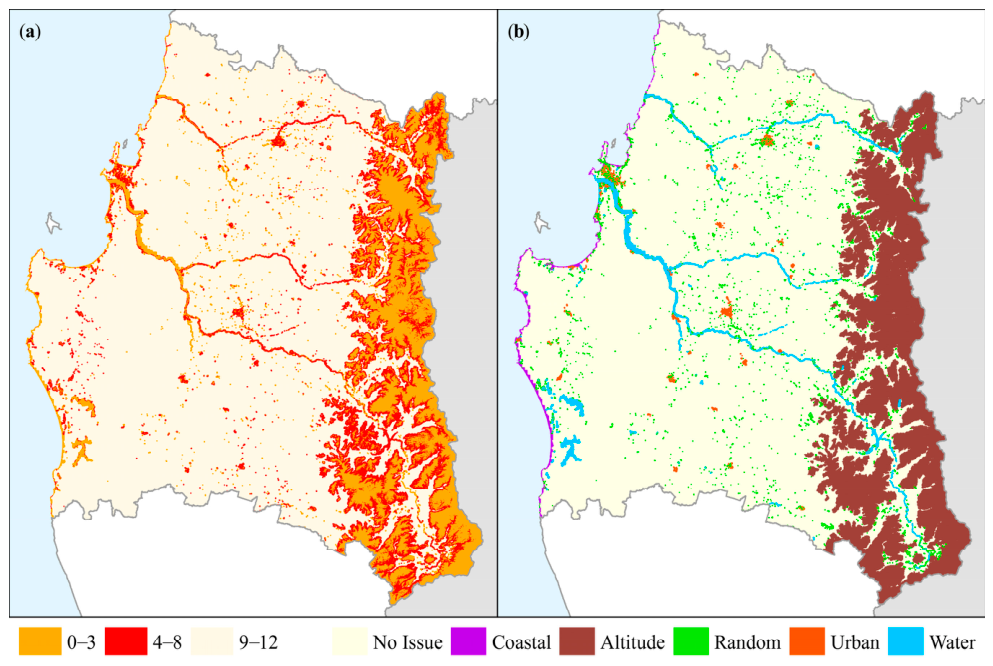
Figure A3. Effective data availability after mosaic assembly. (a) Number of periods with valid data; (b) Main causes of data gaps.
Remotesensing 18 02969 g0a3

Appendix A.2. Dependent Variables

Table A5 presents the homogenization and categorization of 27 unpooled LC classes, 12 pooled LC classes, and seven LU classes used in this study. Table A6 reports the temporal reference of each dataset, including direct links to CONAF institutional sources, and the feature labeled as year. Because temporal references were not homogeneous, each labeled year was assigned a likely two-year period aligned with the biennial mosaics, assuming minimal change. Each period was used in two modes: static, using all LC polygons; and dynamic, using only polygons with unchanged LC categories between temporal references.
Table A5. Land-cover (LC) and land-use (LU) categories.
Code 0:
C0.
Unpooled LC categoryCode 1:
C1.
Pooled
LC Category
Code 2:
C2.
Pooled
LU Category
1Permanent agricultural1Permanent agricultural1Agricultural
2Rotating agricultural2Rotating agricultural
3Annual grassland3Improved agricultural
grassland
4Perennial grassland
5Meadow4Natural
meadow
2Natural
meadow
6Meadow steppe
7Scrubland5Scrubland3Scrubland
8Arborescent scrubland
9Undefined adult forest plantation: adult forest plantation; forest plantation with feral forest plantation6Adult forest plantation4Forest
plantation
10Young or harvested forest plantation7Young or harvested f. p.
11Adult native forest8Native
forest
5Native
forest
12Secondary native renewal forest
13Scrubby native forest
14Undefined native forest: native forest; adult native forest with secondary native renewal forest
15Undefined wetland: wetland; Marsh wetland; Ñadi wetland; Vega wetland; another wetland9Wetland6Wetland
16Beach and dune10Water, riverbank
and shore
17Riverbank
18River
19Lentic water body: water body; lake, lagoon, reservoir and dam
20Urban and industrial11Urban
and industrial
7Without
vegetation
21City, town and industrial zone
22Industrial mining
23Rocks without vegetation12Without
vegetation
24Altitudinal gradient without vegetation
25Scoria without vegetation
26Landslide without vegetation
27Snow and glacier: snow and glacier; snow; glacier
To clean polygon datasets and reduce edge-related confusion, polygons smaller than 0.5 ha were discarded and inner borders were removed over 45 m. Each dataset version (Table A6) was divided into four polygon subsets with progressively smaller minimum areas (i.e., 100, 10, 1, and 0 ha). In parallel, four random point subsamples were generated across the study area using progressively smaller minimum distances (i.e., 900, 600, 400, and 300 m), excluding points near previous subsamples. Each point subsample was intersected with its corresponding polygon subset to extract LC features. The four resulting subsamples were then merged and coded by time reference. Table A7 summarizes the static and dynamic subdataset combinations used to extract observations. Finally, all biennial samples were merged into a complete point sample and labeled by period.
Table A6. Land-cover (LC) polygonal datasets.
Dataset Name
or Source
Labeled
Year
Likely
Characterized
Period
Static Assumed Period
(Recent Past)
Dynamic Assumed Period
(Inter-Statics Periods)
YearsCodeYearsCode
“...period 2013–2016”
[42]
https://ide.minagri.gob.cl/descarga-de-capas-shp/planificacion-catastral
19971995–19961995–1996T1 (not used)
1997–2004T1-T2
20082006–20072005–2006 †T2
2007–2010T2-T3
20142012–20132011–2012 †T3 (not used)
2013–2014Not used
20172015–20162015–2016Not used
“...period 2001–2019”
[43]
https://ide.minagri.gob.cl/descarga-de-capas-shp/planificacion-catastral
20011999–20001999–2000T4
2001–2010T4-T5
20132011–20122011–2012T5
2013–2013Not used
20162014–20152014–2015Not used
2013–2014T5-T6
20172015–20162015–2016T6
20192017–20182017–2018T7
† = assumed lag; T1–T7 = temporal reference codes. Static periods use one reference; dynamic periods use LC polygons unchanged between two references.
Table A7. Biennial periods and samples.
Biennial PeriodAssumed Period Code
P1 1997–1998T1–T2
P2 1999–2000T1–T2 and T4
P3 2001–2002T1–T2 and T4–T5
P4 2003–2004T1–T2 and T4–T5
P5 2005–2006T2 and T4–T5
P6 2007–2008T2–T3 and T4–T5
P7 2009–2010T2–T3 and T4–T5
P8 2011–2012T5
P9 2013–2014T5–T6
P10 2015–2016T6
P11 2017–2018T7
P12 2019–2020No data
T1–T7 = temporal reference codes defined in Table A6.
To assess LC-category distribution, pooled categories were ranked by abundance using the complete point sample and assigned discard percentages. An exponential function connected the least and most abundant categories, assigned 0% and 35% discard, respectively. Within each pooled category, this discard was distributed among unpooled categories using a linear function anchored at the least abundant category, with decreasing slope until the group-specific discard target was reached. If the line became horizontal before reaching the target, it was shifted vertically. Thus, more abundant categories were preferentially reduced until equalization, after which further discard was proportional. Assigned points were then randomly removed from each unpooled category. Period distribution was subsequently assessed using a histogram. The average period abundance was rounded to 500 and multiplied by 1.2 to define a maximum target, ensuring that no period exceeded the average by more than 20%. Points exceeding this target were randomly removed from each period.

Appendix A.3. Comparison Tests

Table A8 summarizes the statistical tests used to analyze the results. Measurements within treatments resemble paired experiments; however, complete pairing is not possible when combinations differ (i.e., B versus BI or BIT) or data are missing. Non-normality detected by Lilliefors tests favored non-parametric tests (Mann–Whitney U or Wilcoxon). Because these tests do not explicitly address heteroscedasticity, Welch or paired t-tests were additionally used when significant heteroscedasticity occurred. Tests assumed their corresponding null conditions of normality, homoscedasticity, no difference, and Ne effect size. Probabilities below 0.001 indicated the corresponding alternatives, including non-normality, heteroscedasticity, significant differences, or S, M, and L effect sizes.
Table A8. Statistical tests.
TypeTestPairedRequires
Normality
Requires
Homoscedasticity
Addresses
Heteroscedasticity
Source
NormalityLilliefors[90]
HomoscedasticityLevene (median-centered)[91]
Fligner–Killeen (median-centered)[92]
ComparisonWelch t (two-sample)[93]
Mann–Whitney U (two-sample rank-sum)[94]
Pairwise t (two-sided)[93]
Wilcoxon (paired two-sample signed-rank)[94]
Effect sizeWelch t (Cohen’s d)[95]
Mann–Whitney U[96]
Pairwise t (Cohen’s d)[95]
Wilcoxon[96]
✓ = applies; ✗ = does not apply; – = not applicable.
This appendix provides detailed results, presenting extensive tables for various performance metrics related to κ. To guide the selection of statistical tests summarized in tables, the following metrics were conducted:
  • The number of total observations (Nº), number of theoretical maximum measurements (N.Max), and percentage of non-missing data ( N % = N º / N . M a x ) were employed as criteria for the selection of paired or unpaired tests.
  • Homoscedasticity assessments: (a) The maximum-to-minimum of SD ratio (Max.SD–Min.SD: max ( S D 1 , S D 2 ) / min ( S D 1 , S D 2 ) ) was employed as a preliminary measure of the variance difference; (b) The Levene and Fligner–Killeen tests were employed as formal tests. They were marked with asterisks indicating statistical significance (*: Probability < 0.001).
  • The difference in the κ Q50 ( Q 50 = Q 50 ( κ 2 ) Q 50 ( κ 1 ) ) was employed as a preliminary measure of treatment difference. Subsequently, when the pairwise difference was calculated, its Q50 ( Q 50 = Q 50 ( κ 2 κ 1 ) ) was employed as well.
  • Comparison (difference) tests: The Welch T, Mann–Whitney U, Pairwise T, and Wilcoxon tests were employed as formal tests. They were marked with a symbol (⁂: best test; **: better test; ·~: less test; ···: least test), indicating the degree of suitability with the data. This suitability is based on normality, homoscedasticity, and non-missing data levels.
  • Test selection and suitability:
    • When complete pairing cannot be achieved due to combinations differing (i.e., B versus BI or B versus BIT), or when any N% is less than 80%, an unpaired test (Welch T or Mann–Whitney U) is employed;
    • When combinations do not differ, and both N% values are greater than or equal to 90%, a paired test (Pairwise T or Wilcoxon) is employed;
    • When combinations do not differ and either N% is at least 80% but below 90%, the paired test is accompanied by the corresponding unpaired test (Welch T or Mann–Whitney U, respectively). The unpaired test is considered less suitable;
    • When both the Levene and Fligner–Killeen tests suggest homoscedasticity, a non-parametric test is employed (Mann–Whitney U or Wilcoxon);
    • When both the Levene and Fligner–Killeen tests suggest heteroscedasticity and the Max.SD–Min.SD ratio is less than or equal to 1.5, the non-parametric test is accompanied by the corresponding parametric test (Welch T or Pairwise T, respectively). The parametric test is considered less suitable;
    • When both the Levene and Fligner–Killeen tests suggest heteroscedasticity and the Max.SD–Min.SD ratio is greater than 1.5, it is considered that a parametric test is equally suitable as a non-parametric test.
  • The confidence interval (CI) lower-limit magnitude was employed as a conservative formal measure of the difference between treatments. Derived from corresponding effect size tests (Table A8), its statistical significance was marked with an asterisk (*: Probability < 0.001). When multiple suitable tests suggested different magnitudes, the smallest effect size was chosen for inclusion in the summary tables.

Appendix A.4. Post-Classification Heuristics

Gaps were filled using a hierarchical approach based on multiple heuristic criteria, without altering previously classified values.
  • First, classifications from temporally adjacent periods were used (when available), following this sequence: from the immediate previous period; from the immediate subsequent period; from the second previous period; from the second subsequent period;
  • Next, index- and threshold-based masks were applied using distances from vector features. Water-feature polygons defined C0.19-lentic-water-body at a distance of zero and C0.15-undefined-wetland below a specified threshold. Glacier polygons were defined as C0.27-snow-and-glacier at a distance of zero. City polygons were defined as C0.20-urban-and-industrial at a distance of zero and C0.21-city-town-and-industrial-zone below a specified threshold;
  • Then, index- and threshold-based masks were applied to elevation and slope. Values close to zero defined C0.16-beach-and-dune. Increasing values progressively defined C0.13-scrubby-native-forest, C0.7-scrubland, C0.24-altitudinal-gradient-without-vegetation, and C0.27-snow-and-glacier;
  • Finally, gaps were filled using extrapolation with a one-pixel local mode.

Appendix B

Appendix B.1. Color Balancing and RF Hyperparameters

Figure A4 shows color-balancing effects on spectral bands across periods and seasons.
Figure A4. Boxplots of normalized winter and summer spectral bands by periods and color-balancing treatment. Band panels follow Table 2.
Remotesensing 18 02969 g0a4aRemotesensing 18 02969 g0a4b
To provide insight into the challenges associated with calibrating RF hyperparameters, the κ grid was explored (Figure A5).
Figure A5. Validation-κ quantiles across RF-hyperparameter combinations for three representative treatments. Columns: (a) 12.5-No-B, lowest-performing; (b) 100-Yes-BI, nearest the overall average; (c) 100-Yes-BIT, highest-performing. Grid dimensions are bag fraction, number of trees, and variables per split. 12.5, 100 = 12.5%, 100% observations; No, Yes = color-unbalanced, -balanced; B = bands; BI = B + indices; BIT = BI + territorial variables.
Remotesensing 18 02969 g0a5aRemotesensing 18 02969 g0a5b

Appendix B.2. Treatment Performances

Table A9 provides validation statistics for grouped treatments, showing the effect-size magnitudes between neighboring groups. Theoretically, combining RF hyperparameters results in a maximum of 924 combinations for the B version treatments and 1584 combinations for the BI and BIT versions. To explain the calculation of N.Max for the grouped treatments, consider the following example for the Obs 12.5 group: 2|color-balanced version| × (924|observation B| + 2 × 1584|observation BI or BIT|) = 8184. As all individual training measurements exceeded 0.9 and no significant overall or group variability was observed, only training-κ Q50 is reported.
Table A9. Statistics of validation-κ for grouped treatments.
ObsBalVarComparisonMinQ50MaxAvgSDN.MaxN%WCVκATraining-κ Q50
12.5 L * 0.3060.4230.5820.4420.068818481841000.3770.996
25 L *0.3480.4560.6350.4990.086818481841000.3670.995
50 L *0.3740.5040.7690.5690.124818481841000.3740.991
100 0.4270.5430.8200.6260.13873928184900.3580.985
No L * 0.3060.4740.8140.5120.1321592216368970.3680.984
Yes 0.3390.5280.8200.5510.1191602216368980.3700.981
BNe * 0.3060.4440.5580.4460.05470957392960.3720.990
BIL *0.3280.4510.5550.4530.0491224812672970.3680.990
BIT 0.4180.6290.8200.6560.1061260112672990.3040.995
12.5No L * 0.3060.3800.5180.4170.060409240921000.3720.997
12.5Yes 0.3390.4270.5820.4680.066409240921000.3820.997
25No L * 0.3480.4260.6330.4860.093409240921000.3540.998
25Yes 0.3850.4600.6350.5110.077409240921000.3760.995
50No L * 0.3740.4570.7490.5480.129409240921000.3770.990
50Yes 0.4290.5080.7690.5900.115409240921000.3720.991
100No L * 0.4270.4950.8140.6100.14636464092890.3660.985
100Yes 0.4730.5470.8200.6420.12737464092920.3490.985
12.5 BS * 0.3060.3800.4420.3870.028184818481000.3860.997
12.5 BIL *0.3280.3900.4400.3970.025316831681000.3840.997
12.5 BIT 0.4180.5110.5820.5200.032316831681000.3150.997
25 BNe * 0.3480.4200.4820.4280.029184818481000.3760.998
25 BIL *0.3710.4310.4670.4340.018316831681000.3540.998
25 BIT 0.5050.6080.6350.6040.019316831681000.3030.998
50 BS * 0.3740.4550.5260.4680.033184818481000.3630.990
50 BIL *0.4130.4710.5180.4760.026316831681000.3640.990
50 BIT 0.5890.7260.7690.7200.032316831681000.2990.990
100 BNe * 0.4270.5050.5580.5090.03015511848840.3540.985
100 BIL *0.4550.5160.5550.5130.02627443168870.3530.982
100 BIT 0.6480.7930.8200.7850.02830973168980.2950.985
Obs = observation %; Bal = color balancing (No, Yes = unbalanced, balanced); Var = predictor set (B = bands, BI = B + indices, BIT = BI + territorial variables); Comparison = adjacent-treatment effect size (* = statistical significance, Ne, S, M, L = negligible, small, moderate, large); Min = minimum; Q50 = median; Max = maximum; Avg = average; SD = standard deviation; Nº, N.Max, N% = available, theoretical maximum, non-missing % measurements; WCVκA = weighted coefficient of variation by κ averaged.
Table A10 summarizes the comparisons of validation-κ for grouped treatments.
Table A10. Comparison tests of validation-κ among grouped treatments.
Comparison Groups12N%1N%2Homoscedastic∆Q50
Q50∆
DifferenceCI Lower-Limit
Magnitude
12.5–2581848184100100(1) 1.272
(2) * (3) *
0.033
0.047
(6) **Large *
(7) ⁂
25–5081848184100100(1) 1.438
(2) * (3) *
0.048
0.051
(6) **Large *
(7) ⁂
50–100739273929090(1) 1.110
(2) * (3) *
0.039
0.044
(6) **Large *
(7) ⁂
No–Yes15922159229797(1) 1.103
(2) * (3) *
0.054
0.044
(6) **Large *
(7) ⁂
B–BI7095122489697(1) 1.094
(2) * (3) *
0.007
0.008
(4) **Negligible *
(5) ⁂Small *
BI–BIT12248122489797(1) 2.163
(2) * (3) *
0.178
0.191
(6) ⁂Large *
(7) ⁂
12.5-No–12.5-Yes40924092100100(1) 1.090
(2) * (3) *
0.047
0.050
(6) **Large *
(7) ⁂
25-No–25-Yes40924092100100(1) 1.209
(2) * (3) *
0.035
0.026
(6) **Large *
(7) ⁂
50-No–50-Yes40924092100100(1) 1.122
(2) * (3) *
0.051
0.046
(6) **Large *
(7) ⁂
100-No–100-Yes364637468992(1) 1.156
(2) * (3) *
0.051
0.044
(4) ···Negligible *
(5)·~Moderate *
364636468989(6) **Large *
(7) ⁂
12.5-B–12.5-BI18483168100100(1) 1.156
(2) * (3) *
0.010
0.009
(4) **Small *
(5) ⁂
25-B–25-BI18483168100100(1) 1.575
(2) * (3) *
0.011
0.007
(4) ⁂Negligible *
(5) ⁂Small *
50-B–50-BI18483168100100(1) 1.281
(2) * (3) *
0.016
0.010
(4) **Small *
(5) ⁂
100-B–100-BI155127448487(1) 1.173
(2) * (3) *
0.010
0.005
(4) **Negligible *
(5) ⁂Small *
12.5-BI–12.5-BIT31683168100100(1) 1.307
(2) * (3) *
0.122
0.123
(6) **Large *
(7) ⁂
25-BI–25-BIT31683168100100(1) 1.046
(2) * (3) *
0.177
0.168
(6) **Large *
(7) ⁂
50-BI–50-BIT31683168100100(1) 1.212
(2) (3)
0.255
0.249
(7) ⁂Large *
100-BI–100-BIT274430978798(1) 1.104
(2) * (3) *
0.278
0.269
(4) ···Large *
(5)·~
274427448787(6) **
(7) ⁂
Treatment codes follow Table A9. Subscripts 1 and 2 identify the compared groups. Nº, N% = available, non-missing % measurements; ΔQ50 = difference between medians; Q50Δ = median paired difference; CI = confidence interval; * = statistical significance. Test: (1) Max.SD–Min.SD ratio; (2) Levene; (3) Fligner–Killeen; (4) Welch T; (5) Mann–Whitney U; (6) Pairwise T; (7) Wilcoxon. Suitability: ⁂ = Best; ** = Better; ·~ = Less; ··· = Least.
Table A11 summarizes the comparisons of differences in validation-κ for grouped treatments.
Table A11. Comparison test of validation-κ differences among grouped treatments.
Comparison Groups12N%1N%2Homoscedastic∆Q50DifferenceCI Lower-Limit
Magnitude
[12.5–25]–[25–50]81848184100100(1) 1.338
(2) * (3) *
0.003(6) **Small *
(7) ⁂
[12.5–25]–[50–100]739273929090(1) 2.121
(2) * (3) *
−0.003(6) ⁂−Small *
(7) ⁂
[25–50]–[50–100]739273929090(1) 2.839
(2) * (3) *
−0.006(6) ⁂−Moderate *
(7) ⁂−Large *
[B–BI]–[BI–BIT]7089122489697(1) 4.375
(2) * (3) *
0.183(4) ⁂Large *
(5) ⁂
[12.5-No–12.5-Yes]–
[25-No–25-Yes]
40924092100100(1) 1.807
(2) * (3) *
−0.024(6) ⁂−Large *
(7) ⁂
[12.5-No–12.5-Yes]–
[50-No–50-Yes]
40924092100100(1) 1.426
(2) * (3) *
−0.004(6) **−Small *
(7) ⁂
[12.5-No–12.5-Yes]–
[100-No–100-Yes]
4092364610089(1) 1.844
(2) * (3) *
−0.006(4)·~−Large *
(5)·~−Moderate *
364636468989(6) ⁂
(7) ⁂
[25-No–25-Yes]–
[50-No–50-Yes]
40924092100100(1) 1.267
(2) * (3) *
0.020(6) **Large *
(7) ⁂
[25-No–25-Yes]–
[100-No–100-Yes]
4092364610089(1) 1.020
(2) * (3) *
0.018(4) ···Small *
(5)·~
364636468989(6) **Large *
(7) ⁂
[50-No–50-Yes]–
[100-No–100-Yes]
4092364610089(1) 1.293
(2) * (3) *
−0.002(4) ···−Small *
(5)·~
364636468989(6) **−Moderate *
(7) ⁂−Large *
[12.5-BI–12.5-BIT]–
[25-BI–25-BIT]
31683168100100(1) 1.371
(2) * (3) *
0.045(6) **Large *
(7) ⁂
[12.5-BI–12.5-BIT]–
[50-BI–50-BIT]
31683168100100(1) 2.033
(2) * (3) *
0.126(6) ⁂Large *
(7) ⁂
[12.5-BI–12.5-BIT]–
[100-BI–100-BIT]
3168274410087(1) 2.019
(2) * (3) *
0.146(4)·~Large *
(5)·~
274427448787(6) ⁂
(7) ⁂
[25-BI–25-BIT]–
[50-BI–50-BIT]
31683168100100(1) 1.483
(2) * (3) *
0.081(6) ⁂Large *
(7) ⁂
[25-BI–25-BIT]–
[100-BI–100-BIT]
3168274410087(1) 1.473
(2) * (3) *
0.101(4)·~Large *
(5)·~
274427448787(6) ⁂
(7) ⁂
[50-BI–50-BIT]–
[100-BI–100-BIT]
3168274410087(1) 1.007
(2) (3)
0.020(5)·~Moderate *
274427448787(7) ⁂Large *
Follows Table A10 format.
Table A12 provides validation statistics for ungrouped treatments and follows Table A9 format.
Table A13 summarizes the comparisons of validation-κ between neighboring ungrouped treatments; both arranged according to their Q50 values.
Table A12. Statistics of validation-κ for ungrouped treatments ordered by Q50.
ObsBalVarComparisonMinQ50MaxAvgSDN.MaxN%WCVκATraining-κ
Q50
12.5NoBM* 0.3060.3650.3890.3630.0139249241000.3990.994
12.5NoBIL*0.3280.3760.3940.3740.009158415841000.3710.994
25NoBL*0.3480.4070.4330.4040.0139249241000.3750.998
12.5YesBS*0.3390.4150.4420.4120.0169249241000.3750.997
12.5YesBINe0.3760.4210.4400.4200.010158415841000.3960.997
25NoBIL*0.3710.4220.4370.4190.010158415841000.3280.998
50NoBM*0.3740.4410.4570.4380.0139249241000.3650.988
25YesBIS*0.4020.4520.4670.4500.010158415841000.3680.995
50NoBIS*0.4130.4530.4740.4510.009158415841000.3650.990
25YesBL*0.3850.4560.4820.4530.0169249241000.3760.995
100NoBM*0.4270.4830.5000.4810.011757924820.3560.984
100NoBINe*0.4550.4900.5070.4890.00813461584850.3600.985
12.5NoBITS*0.4180.4930.5180.4910.014158415841000.3080.997
50YesBNe*0.4290.5010.5260.4980.0159249241000.3620.991
50YesBIL*0.4590.5020.5180.5000.008158415841000.3620.990
100YesBINe0.5010.5380.5550.5370.00913981584880.3380.985
100YesBM*0.4730.5390.5580.5370.012794924860.3500.984
12.5YesBITL*0.4710.5500.5820.5480.015158415841000.3200.997
25NoBITS*0.5050.6060.6330.6010.022158415841000.2970.998
25YesBITL*0.5370.6100.6350.6060.015158415841000.3070.995
50NoBITL*0.5890.7160.7490.7080.030158415841000.3000.990
50YesBITL*0.6180.7390.7690.7320.028158415841000.2990.991
100NoBITL*0.6480.7880.8140.7790.03015431584970.2970.985
100YesBIT 0.6840.7990.8200.7910.02515541584980.2940.984
Follows Table A9 format.
Table A13. Comparison tests of validation-κ among ungrouped treatments ordered by Q50.
Comparison Groups12N%1N%2Homoscedastic∆Q50DifferenceCI Lower-Limit
Magnitude
12.5-No-B–12.5-No-BI9241584100100(1) 1.415
(2) * (3) *
0.011(4) **Large *
(5) ⁂Moderate *
12.5-No-BI–25-No-B9241584100100(1) 1.430
(2) * (3) *
0.031(4) **Large *
(5) ⁂
25-No-B–12.5-Yes-B924924100100(1) 1.223
(2) * (3) *
0.008(6) **Large *
(7) ⁂
12.5-Yes-B–12.5-Yes-BI9241584100100(1) 1.638
(2) * (3) *
0.006(4) ⁂Moderate *
(5) ⁂Small *
12.5-Yes-BI–25-No-BI15841584100100(1) 1.041
(2) (3)
0.001(7) ⁂Negligible or Small
25-No-BI–50-No-B9241584100100(1) 1.301
(2) * (3) *
0.019(4) **Large *
(5) ⁂
50-No-B–25-Yes-BI9241584100100(1) 1.326
(2) * (3) *
0.011(4) **Large *
(5) ⁂Moderate *
25-Yes-BI–50-No-BI15841584100100(1) 1.069
(2) (3)
0.001(7) ⁂Small *
50-No-BI–25-Yes-B1584924100100(1) 1.697
(2) * (3) *
0.003(4) ⁂Negligible
(5) ⁂Small *
25-Yes-B–100-No-B75792482100(1) 1.453
(2) * (3) *
0.027(4)·~Large *
(5)·~
7577578282(6) ⁂
(7) ⁂
100-No-B–100-No-BI75713468285(1) 1.371
(2) * (3) *
0.007(4) **Moderate *
(5) ⁂
100-No-BI–12.5-No-BIT1346158485100(1) 1.754
(2) * (3) *
0.004(4)·~Negligible *
(5)·~Small *
134613468585(6) ⁂Negligible *
(7) ⁂Small *
12.5-No-BIT–50-Yes-B1584924100100(1) 1.040
(2) (3)
0.007(5) ⁂Small *
50-Yes-B–50-Yes-BI9241584100100(1) 1.784
(2) * (3) *
0.001(4) ⁂Negligible *
(5) ⁂Small
50-Yes-BI–100-Yes-BI1584139810088(1) 1.060
(2) (3)
0.036(5)·~Large *
139813988888(7) ⁂
100-Yes-BI–100-Yes-B79413988688(1) 1.384
(2) * (3) *
0.001(4) ⁂Negligible
(5) ⁂
100-Yes-B–12.5-Yes-BIT794158486100(1) 1.199
(2) * (3) *
0.011(4) **Moderate *
(5) ⁂
12.5-Yes-BIT–25-No-BIT15841584100100(1) 1.516
(2) * (3) *
0.056(6) ⁂Large *
(7) ⁂
25-No-BIT–25-Yes-BIT15841584100100(1) 1.437
(2) * (3) *
0.004(6) **Small *
(7) ⁂Moderate *
25-Yes-BIT–50-No-BIT15841584100100(1) 1.988
(2) * (3) *
0.106(6) ⁂Large *
(7) ⁂
50-No-BIT–50-Yes-BIT15841584100100(1) 1.106
(2) (3)
0.024(7) ⁂Large *
50-Yes-BIT–100-No-BIT154315439797(1) 1.093
(2) (3)
0.049(7) ⁂Large *
100-No-BIT–100-Yes-BIT154315439797(1) 1.195
(2) * (3) *
0.011(6) **Large *
(7) ⁂
Follows Table A10 format.
Table A14. Comparison test of differences in validation-κ among selected treatments.
Comparison Groups12N%1N%2Homoscedastic∆Q50DifferenceCI Lower-Limit
Magnitude
[12.5-No-BI–12.5-Yes-BIT]–
[25-No-BI–25-Yes-BIT]
15841584100100(1) 1.105
(2) * (3) *
0.014(6) **Large *
(7) ⁂
[12.5-No-BI–12.5-Yes-BIT]–
[50-No-BI–50-Yes-BIT]
15841584100100(1) 2.075
(2) * (3) *
0.113(6) ⁂Large *
(7) ⁂
[12.5-No-BI–12.5-Yes-BIT]–
[100-No-BI–100-Yes-BIT]
1584134610085(1) 1.831
(2) * (3) *
0.134(4)·~Large *
(5)·~
134613468585(6) ⁂
(7) ⁂
[25-No-BI–25-Yes-BIT]–
[50-No-BI–50-Yes-BIT]
15841584100100(1) 2.294
(2) * (3) *
0.099(6) ⁂Large *
(7) ⁂
[25-No-BI–25-Yes-BIT]–
[100-No-BI–100-Yes-BIT]
1584134610085(1) 2.023
(2) * (3) *
0.120(4)·~Large *
(5)·~
134613468585(6) ⁂
(7) ⁂
[50-No-BI–50-Yes-BIT]–
[100-No-BI–100-Yes-BIT]
1584134610085(1) 1.134
(2) * (3) *
0.021(4)···Moderate *
(5)·~
134613468585(6) **Large *
(7)⁂
Follows Table A10 format.
The comparisons of validation-κ for the selected treatments were deemed unnecessary. Observing the treatments within the selected, it can be concluded that the differences between these treatments are all significantly large (Large*). As for the comparisons of differences in validation-κ, Table A14 summarizes them for selected treatments.
To explore the differences between training and validation performance and the impact of pooling categories on performance measurement, Table A15 displays the Q50 and Max values for the selected ungrouped treatments.
Table A15. Q50 and Max of training-κ and validation-κ by category-pooling code.
ObsBalVarTraining-κ Q50 CodeValidation-κ Q50 CodeTraining-κ Max CodeValidation-κ Max Code
012012012012
12.5NoBI0.9940.9970.9980.3760.5000.6700.9971.0001.0000.3940.5080.680
25NoBI0.9981.0001.0000.4220.5200.6560.9981.0001.0000.4370.5360.672
50NoBI0.9900.9970.9970.4530.5500.7110.9900.9970.9970.4740.5630.721
100NoBI0.9850.9970.9970.4900.5860.7350.9850.9970.9970.5070.5980.743
12.5YesBIT0.9970.9990.9990.5500.6360.7520.9970.9990.9990.5820.6630.762
25YesBIT0.9950.9990.9990.6100.6820.7900.9950.9990.9990.6350.7030.807
50YesBIT0.9910.9970.9970.7390.7780.8580.9910.9970.9970.7690.8030.871
100YesBIT0.9840.9970.9970.7990.8480.8990.9850.9970.9970.8200.8680.910
Obs = observation %; Bal = color balancing (No, Yes = color-unbalanced, -balanced); Var = predictor set (BI = bands + indices, BIT = BI + territorial variables); Q50 = median; Max = maximum; Code 0, 1 = unpooled, pooled LC categories; Code 2 = pooled LU categories.

Appendix B.3. Land Use

Table A16 presents the transition matrix between P1 and P12.
Table A16. Transition matrix from P1 to P12.
Period P1 P12
Code 2C2.1C2.2C2.3C2.4C2.5C2.6C2.7Total
C2.120.730.050.433.390.170.250.2325.24
C2.20.060.970.160.010.150.010.051.41
C2.30.330.066.880.511.130.090.069.06
P12C2.45.920.040.9625.652.190.230.0935.07
C2.50.230.050.612.3915.610.030.0218.93
C2.60.120.000.050.120.051.490.021.85
C2.70.360.040.110.140.050.037.728.44
P1Total27.741.209.2132.2119.342.128.18100.00
P1 = 1997–1998; P12 = 2019–2020; C2.1 = agricultural; C2.2 = natural meadow; C2.3 = scrubland; C2.4 = forest plantation; C2.5 = native forest; C2.6 = wetland; C2.7 = without vegetation. Rows represent P12 and columns represent P1. Values are % of the study area.
In Table A17, values underwent varying degrees of processing: some were directly extracted, others were visually approximated from figures, and others were recalculated from gridded datasets.
Table A17. Annual exponential land-use (LU) change rates (% year−1, base e ).
Group (a, b, c),
Zone or
Statistic
Intersection
/Union
Area %
Year MinYear MaxAvg
Year
C2.1
Rate
C2.2
Rate
C2.3
Rate
C2.4
Rate
C2.5
Rate
C2.6
Rate
C2.7
Rate
C2.4-C2.5
Rate
Source
(a) 1975–2001
Our north coast2 †197519901982.5−1.98 0.707.90−5.06 0.15[49]
Our north-central coast6 †197519981986.5−1.96 3.12−1.51 0.97[32]
Our central area48 †197920001989.5−1.320.00−2.8010.5−1.60 2.24[30]
South-central Chile24198620011993.5−1.580.26 4.30−0.51 0.57[5]
Biobío Region73198620011993.5−3.51 2.854.51−2.41 0.87[5] †
Araucanía Region23198620011993.5−2.02 0.3110.7−0.53 1.29[5] †
Our north coast2 †199020001995.04.65 −5.447.83−3.63 4.95[49]
All Chile7199220011996.5−1.28 3.31 0.08[6]
Avg (group a)231983.61999.01991.3−1.130.13−0.886.52−2.18 1.39
Nº (group a)888882587008
(b) 1997–2020
South-central Chile24199720112004.0 0.970.12 0.38[5]
Our same area100 ‡199720152006.0−0.83−0.150.31 −3.391.130.17[53] ‡
Our north-central coast6 †199820142006.0−2.75 0.94−2.52 −0.02[32]
South-central Chile24200120112006.01.60 −2.422.24−0.06 0.67[5]
Biobío Region73200120112006.01.67 −3.050.38−0.05 0.21[5] †
Araucanía Region23200120112006.01.50 −2.011.82−0.87 0.00[5] †
Our same area100 ‡199920182008.5−0.72−2.272.650.30−1.51−0.600.69−0.73[51] ‡
Our same area100 ‡200020202010.0−0.540.000.270.95−0.460.13−0.370.22[52] ‡
Andalién river basin2200820152011.5−6.64 10.2−0.450.218.450.49−0.30[50]
Andalién river basin2201520202017.5−5.22 −11.72.71−3.42−13.717.31.46[50]
Avg (group b)452001.72014.62008.2−1.32−0.81−0.721.10−0.95−1.813.850.21
Nº (group b)10101010938995510
(c) 1997.5–2019.5
Our area (P1, P12)1001997.52019.52008.5−0.430.71−0.070.39−0.10−0.620.140.21This study
Our area (P1, ···, P12)1001997.52019.52008.5−0.570.62−0.130.52−0.07−0.740.100.31This study
Intersection/Union Area = spatial intersection divided by spatial union; Min = minimum; Max = maximum; Avg = average; C2.1 = agricultural; C2.2 = natural meadow; C2.3 = scrubland; C2.4 = forest plantation; C2.5 = native forest; C2.6 = wetland; C2.7 = without vegetation; Nº = number of estimates; † = visually approximated; ‡ = derived directly from gridded datasets.
Figure A6 illustrates these two periods to visualize the first-to-last criterion.
Figure A6. LU maps for the first and last biennial periods. (a) P1, 1997–1998; (b) P12, 2019–2020.
Remotesensing 18 02969 g0a6

References

  1. Hansen, M.C.; Loveland, T.R. A Review of Large Area Monitoring of Land Cover Change Using Landsat Data. Remote Sens. Environ. 2012, 122, 66–74. [Google Scholar] [CrossRef] [Scilit]
  2. Wulder, M.A.; Roy, D.P.; Radeloff, V.C.; Loveland, T.R.; Anderson, M.C.; Johnson, D.M.; Healey, S.; Zhu, Z.; Scambos, T.A.; Pahlevan, N.; et al. Fifty Years of Landsat Science and Impacts. Remote Sens. Environ. 2022, 280, 113195. [Google Scholar] [CrossRef] [Scilit]
  3. Gorelick, N.; Hancher, M.; Dixon, M.; Ilyushchenko, S.; Thau, D.; Moore, R. Google Earth Engine: Planetary-Scale Geospatial Analysis for Everyone. Remote Sens. Environ. 2017, 202, 18–27. [Google Scholar] [CrossRef] [Scilit]
  4. Zhu, Z.; Wang, S.; Woodcock, C.E. Improvement and Expansion of the Fmask Algorithm: Cloud, Cloud Shadow, and Snow Detection for Landsats 4–7, 8, and Sentinel 2 Images. Remote Sens. Environ. 2015, 159, 269–277. [Google Scholar] [CrossRef] [Scilit]
  5. Heilmayr, R.; Echeverría, C.; Fuentes, R.; Lambin, E.F. A Plantation-Dominated Forest Transition in Chile. Appl. Geogr. 2016, 75, 71–82. [Google Scholar] [CrossRef] [Scilit]
  6. Benavidez-Silva, C.; Jensen, M.; Pliscoff, P. Future Scenarios for Land Use in Chile: Identifying Drivers of Change and Impacts over Protected Area System. Land 2021, 10, 408. [Google Scholar] [CrossRef] [Scilit]
  7. Hermosilla, T.; Wulder, M.A.; White, J.C.; Coops, N.C. Land Cover Classification in an Era of Big and Open Data: Optimizing Localized Implementation and Training Data Selection to Improve Mapping Outcomes. Remote Sens. Environ. 2022, 268, 112780. [Google Scholar] [CrossRef] [Scilit]
  8. Gupta, R.; Nanda, S.J. Cloud Detection in Satellite Images with Classical and Deep Neural Network Approach: A Review. Multimed. Tools Appl. 2022, 81, 31847–31880. [Google Scholar] [CrossRef] [Scilit]
  9. Li, Z.; Shen, H.; Weng, Q.; Zhang, Y.; Dou, P.; Zhang, L. Cloud and Cloud Shadow Detection for Optical Satellite Imagery: Features, Algorithms, Validation, and Prospects. ISPRS J. Photogramm. Remote Sens. 2022, 188, 89–108. [Google Scholar] [CrossRef] [Scilit]
  10. Google. Landsat Algorithms|Landsat Processing Methods|Simple Cloud Score. Available online: https://developers.google.com/earth-engine/guides/landsat#simple-cloud-score (accessed on 31 December 2020).
  11. Google. Ee.Algorithms.Landsat.SimpleCloudScore. Available online: https://developers.google.com/earth-engine/apidocs/ee-algorithms-landsat-simplecloudscore (accessed on 31 December 2021).
  12. Helmer, E.H.; Ruefenacht, B. Cloud-Free Satellite Image Mosaics with Regression Trees and Histogram Matching. Photogramm. Eng. Remote Sens. 2005, 71, 1079–1089. [Google Scholar] [CrossRef] [Scilit]
  13. Chang, S.-K.; Wong, Y.-W. Optimal Histogram Matching by Monotone Gray Level Transformation. Commun. ACM 1978, 21, 835–840. [Google Scholar] [CrossRef] [Scilit]
  14. Grundland, M.; Dodgson, N.A. Color Histogram Specification by Histogram Warping. In Color Imaging X: Processing, Hardcopy, and Applications; Eschbach, R., Marcu, G.G., Eds.; SPIE: Bellingham, WA, USA, 2005; Volume 5667, pp. 610–621. [Google Scholar] [CrossRef] [Scilit]
  15. Wulder, M.A.; Coops, N.C.; Roy, D.P.; White, J.C.; Hermosilla, T. Land Cover 2.0. Int. J. Remote Sens. 2018, 39, 4254–4284. [Google Scholar] [CrossRef] [Scilit]
  16. Mellor, A.; Boukir, S.; Haywood, A.; Jones, S. Exploring Issues of Training Data Imbalance and Mislabelling on Random Forest Performance for Large Area Land Cover Classification Using the Ensemble Margin. ISPRS J. Photogramm. Remote Sens. 2015, 105, 155–168. [Google Scholar] [CrossRef] [Scilit]
  17. Zhu, Z.; Gallant, A.L.; Woodcock, C.E.; Pengra, B.; Olofsson, P.; Loveland, T.R.; Jin, S.; Dahal, D.; Yang, L.; Auch, R.F. Optimizing Selection of Training and Auxiliary Data for Operational Land Cover Classification for the LCMAP Initiative. ISPRS J. Photogramm. Remote Sens. 2016, 122, 206–221. [Google Scholar] [CrossRef] [Scilit]
  18. Bera, D.; Das Chatterjee, N.; Bera, S.; Ghosh, S.; Dinda, S. Comparative Performance of Sentinel-2 MSI and Landsat-8 OLI Data in Canopy Cover Prediction Using Random Forest Model: Comparing Model Performance and Tuning Parameters. Adv. Space Res. 2023, 71, 4691–4709. [Google Scholar] [CrossRef] [Scilit]
  19. Chen, B.; Huang, B.; Xu, B. Multi-Source Remotely Sensed Data Fusion for Improving Land Cover Classification. ISPRS J. Photogramm. Remote Sens. 2017, 124, 27–39. [Google Scholar] [CrossRef] [Scilit]
  20. Belgiu, M.; Drăgu, L. Random Forest in Remote Sensing: A Review of Applications and Future Directions. ISPRS J. Photogramm. Remote Sens. 2016, 114, 24–31. [Google Scholar] [CrossRef] [Scilit]
  21. Rodriguez-Galiano, V.F.; Ghimire, B.; Rogan, J.; Chica-Olmo, M.; Rigol-Sanchez, J.P. An Assessment of the Effectiveness of a Random Forest Classifier for Land-Cover Classification. ISPRS J. Photogramm. Remote Sens. 2012, 67, 93–104. [Google Scholar] [CrossRef] [Scilit]
  22. Behnamian, A.; Millard, K.; Banks, S.N.; White, L.; Richardson, M.; Pasher, J. A Systematic Approach for Variable Selection with Random Forests: Achieving Stable Variable Importance Values. IEEE Geosci. Remote Sens. Lett. 2017, 14, 1988–1992. [Google Scholar] [CrossRef] [Scilit]
  23. Sun, J.; Ongsomwang, S. Optimal Parameters of Random Forest for Land Cover Classification with Suitable Data Type and Dataset on Google Earth Engine. Front. Earth Sci. 2023, 11, 1188093. [Google Scholar] [CrossRef] [Scilit]
  24. Casanova, M.; Salazar, O.; Seguel, O.; Luzio, W. General Chile Overview. In The Soils of Chile; Springer: Dordrecht, The Netherlands, 2013; pp. 1–24. [Google Scholar]
  25. Fernández, B.; Gironás, J. (Eds.) Water Resources of Chile; Springer International Publishing: Cham, Switzerland, 2021; Volume 8. [Google Scholar]
  26. Cecioni, A.; Pineda, V. Geology and Geomorphology of Natural Hazards and Human-Induced Disasters in Chile. In Developments in Earth Surface Processes; Latrubesse, E.M., Ed.; Elsevier: Amsterdam, The Netherlands, 2009; Volume 13, pp. 379–413. [Google Scholar]
  27. Barry, R.G. The Wet Andes. In Mountain Weather and Climate; Cambridge University Press: New York, NY, USA, 2008; pp. 425–426. [Google Scholar]
  28. Miranda, A.; Altamirano, A.; Cayuela, L.; Pincheira, F.; Lara, A. Different Times, Same Story: Native Forest Loss and Landscape Homogenization in Three Physiographical Areas of South-Central of Chile. Appl. Geogr. 2015, 60, 20–28. [Google Scholar] [CrossRef] [Scilit]
  29. Zhao, Y.; Feng, D.; Yu, L.; Wang, X.; Chen, Y.; Bai, Y.; Hernández, H.J.; Galleguillos, M.; Estades, C.; Biging, G.S.; et al. Detailed Dynamic Land Cover Mapping of Chile: Accuracy Improvement by Integrating Multi-Temporal Data. Remote Sens. Environ. 2016, 183, 170–185. [Google Scholar] [CrossRef] [Scilit]
  30. Aguayo, M.; Pauchard, A.; Azócar, G.; Parra, O. Land Use Change in the South Central Chile at the End of the 20th Century. Understanding the Spatio-Temporal Dynamics of the Landscape. Rev. Chil. Hist. Nat. 2009, 82, 361–374. [Google Scholar] [CrossRef] [Scilit]
  31. Torres, R.; Azócar, G.; Rojas, J.; Montecinos, A.; Paredes, P. Vulnerability and Resistance to Neoliberal Environmental Changes: An Assessment of Agriculture and Forestry in the Biobio Region of Chile (1974–2014). Geoforum 2015, 60, 107–122. [Google Scholar] [CrossRef] [Scilit]
  32. Uribe, S.V.; Estades, C.F.; Radeloff, V.C. Pine Plantations and Five Decades of Land Use Change in Central Chile. PLoS ONE 2020, 15, e0230193. [Google Scholar] [CrossRef] [Scilit]
  33. USGS. USGS Landsat 5 Surface Reflectance Tier 1 [Data Set Deprecated]. Available online: https://developers.google.com/earth-engine/datasets/catalog/LANDSAT_LT05_C01_T1_SR (accessed on 31 December 2020).
  34. USGS. USGS Landsat 7 Surface Reflectance Tier 1 [Data Set Deprecated]. Available online: https://developers.google.com/earth-engine/datasets/catalog/LANDSAT_LE07_C01_T1_SR (accessed on 31 December 2020).
  35. USGS. USGS Landsat 8 Surface Reflectance Tier 1 [Data Set Deprecated]. Available online: https://developers.google.com/earth-engine/datasets/catalog/LANDSAT_LC08_C01_T1_SR (accessed on 31 December 2020).
  36. Potapov, P.; Hansen, M.C.; Kommareddy, I.; Kommareddy, A.; Turubanova, S.; Pickens, A.; Adusei, B.; Tyukavina, A.; Ying, Q. Landsat Analysis Ready Data for Global Land Cover and Land Cover Change Mapping. Remote Sens. 2020, 12, 426. [Google Scholar] [CrossRef] [Scilit]
  37. Lavender, S.; Lavender, A. Basic Remote Sensing Using Landsat Data. In Practical Handbook of Remote Sensing; CRC Press: Boca Raton, FL, USA, 2023; pp. 33–51. [Google Scholar]
  38. Richards, J.A. Histogram Matching. In Remote Sensing Digital Image Analysis; Springer: Cham, Switzerland, 2022; pp. 122–126. [Google Scholar]
  39. Liu, J.G.; Mason, P.J. Point Operations (Contrast Enhancement). In Image Processing and GIS for Remote Sensing: Techniques and Applications; Wiley-Blackwell: Chichester, UK, 2016; pp. 9–19. [Google Scholar]
  40. Neumann, L.; Neumann, A. Color Style Transfer Techniques Using Hue, Lightness and Saturation Histogram Matching. In Computational Aesthetics 2005. EG Workshop on Computational Aesthetics in Graphics, Visualization and Imaging, Girona, Spain, 18–20 May 2005; Neumann, L., Sbert, M., Gooch, B., Purgathofer, W., Eds.; The Eurographics Association: Aire-la-Ville, Switzerland, 2005; pp. 111–122. [Google Scholar]
  41. Albornoz, A.; Alegría, D.; Cortés, F.; Moya, J. Protocolo Metodológico Para La Elaboración de Cartografías de Usos Y Cambios de Usos de La Tierra; FAO & MINAGRI: Santiago, Chile, 2021. [Google Scholar]
  42. CONAF. Planificación Catastral | Monitoreos de Cambios de Usos de La Tierra|Cartografía Temática de Cambio de Uso de La Tierra (Regiones Del Biobío y La Araucanía) Para El Periodo 2013–2016 [Data Sets: Cambio_uso_tierra_periodo_2013_2016_reg08; Cambio_uso_tierra_periodo_2013_2016_reg09]. Available online: https://web.archive.org/web/20200811092310/http://ide.minagri.gob.cl/geoweb/2019/11/22/planificacion-catastral (accessed on 31 December 2020).
  43. CONAF. Planificación Catastral|Monitoreos de Cambios de Usos de La Tierra|Cartografía Temática de Cambio de Uso de La Tierra (Regiones Del Biobío, La Araucanía y Ñuble) Para El Periodo 2001–2019 [Data Sets: Mh_cambio_uso_tierra_reg08; Mh_cambio_uso_tierra_reg09; Mh_cambio_uso_tierra_reg16]. Available online: https://web.archive.org/web/20210613203949/https://ide.minagri.gob.cl/geoweb/2019/11/22/planificacion-catastral (accessed on 30 June 2021).
  44. Google. Ee.Classifier.SmileRandomForest. Available online: https://developers.google.com/earth-engine/apidocs/ee-classifier-smilerandomforest (accessed on 30 June 2022).
  45. Montesinos López, O.A.; Montesinos López, A.; Crossa, J. Overfitting, Model Tuning, and Evaluation of Prediction Performance. In Multivariate Statistical Machine Learning Methods for Genomic Prediction; Springer: Cham, Switzerland, 2022; pp. 109–139. [Google Scholar]
  46. Richards, J.A. Image Classification in Practice. In Remote Sensing Digital Image Analysis; Springer: Cham, Switzerland, 2022; pp. 447–502. [Google Scholar]
  47. Haifeng, L. Smile.Classification|Class RandomForest. Available online: https://haifengl.github.io/api/java/smile/classification/RandomForest.html (accessed on 31 August 2025).
  48. Loecher, M. Unbiased Variable Importance for Random Forests. Commun. Stat. Theory Methods 2022, 51, 1413–1425. [Google Scholar] [CrossRef] [Scilit]
  49. Echeverria, C.; Coomes, D.; Salas, J.; Rey-Benayas, J.M.; Lara, A.; Newton, A. Rapid Deforestation and Fragmentation of Chilean Temperate Forests. Biol. Conserv. 2006, 130, 481–494. [Google Scholar] [CrossRef] [Scilit]
  50. Pereira, C.O.; Escanilla-Minchel, R.; González, A.C.; Alcayaga, H.; Aguayo, M.; Arias, M.A.; Flores, A.N. Assessment of Future Land Use/Land Cover Scenarios on the Hydrology of a Coastal Basin in South-Central Chile. Sustainability 2022, 14, 16363. [Google Scholar] [CrossRef] [Scilit]
  51. Galleguillos, M.; Ceballos-Comisso, A.; Gimeno, F.; Zambrano-Bigiarini, M. CLDynamicLandCover [Data Set Version 3]. Zenodo. Available online: https://zenodo.org/records/13153631 (accessed on 31 May 2025).
  52. MapBiomas. MapBiomas Chile Project—Collection 2.0 of the Annual Series of Land Cover and Land Use Maps of Chile [Data Set]. Available online: https://chile.mapbiomas.org (accessed on 30 June 2025).
  53. C3S. Land Cover Classification Gridded Maps from 1992 to Present Derived from Satellite Observation [Data Set Global Land Cover Maps Version 2.0.7]. Copernicus Climate Change Service (C3S), Climate Data Store (CDS). Available online: https://cds.climate.copernicus.eu/datasets/satellite-land-cover?tab=overview (accessed on 30 June 2025).
  54. QGIS.org. QGIS Geographic Information System, version 3.38; QGIS Association: Grüt, Switzerland, 2024. [Google Scholar]
  55. R Core Team. R: A Language and Environment for Statistical Computing, version 4.3.1.; R Foundation for Statistical Computing: Vienna, Austria, 2023. [Google Scholar]
  56. Zhu, Z.; Woodcock, C.E. Continuous Change Detection and Classification of Land Cover Using All Available Landsat Data. Remote Sens. Environ. 2014, 144, 152–171. [Google Scholar] [CrossRef] [Scilit]
  57. Ghamisi, P.; Gloaguen, R.; Atkinson, P.M.; Benediktsson, J.A.; Rasti, B.; Yokoya, N.; Wang, Q.; Hofle, B.; Bruzzone, L.; Bovolo, F.; et al. Multisource and Multitemporal Data Fusion in Remote Sensing: A Comprehensive Review of the State of the Art. IEEE Geosci. Remote Sens. Mag. 2019, 7, 6–39. [Google Scholar] [CrossRef] [Scilit]
  58. Chuvieco, E. Physical Principles of Remote Sensing. In Fundamentals of Satellite Remote Sensing: An Environmental Approach; CRC Press: Boca Raton, FL, USA, 2020; pp. 21–58. [Google Scholar]
  59. Li, L.; Li, Y.; Xia, M.; Li, Y.; Yao, J.; Wang, B. Grid Model-Based Global Color Correction for Multiple Image Mosaicking. IEEE Geosci. Remote Sens. Lett. 2021, 18, 2006–2010. [Google Scholar] [CrossRef] [Scilit]
  60. More, A.S.; Rana, D.P. Performance Enrichment through Parameter Tuning of Random Forest Classification for Imbalanced Data Applications. Mater. Today Proc. 2022, 56, 3585–3593. [Google Scholar] [CrossRef] [Scilit]
  61. Ramezan, C.A.; Warner, T.A.; Maxwell, A.E.; Price, B.S. Effects of Training Set Size on Supervised Machine-Learning Land-Cover Classification of Large-Area High-Resolution Remotely Sensed Data. Remote Sens. 2021, 13, 368. [Google Scholar] [CrossRef] [Scilit]
  62. Pelletier, C.; Valero, S.; Inglada, J.; Champion, N.; Marais Sicre, C.; Dedieu, G. Effect of Training Class Label Noise on Classification Performances for Land Cover Mapping with Satellite Image Time Series. Remote Sens. 2017, 9, 173. [Google Scholar] [CrossRef] [Scilit]
  63. Breiman, L. Random Forests. Mach. Learn. 2001, 45, 5–32. [Google Scholar] [CrossRef] [Scilit]
  64. Sheykhmousa, M.; Mahdianpari, M.; Ghanbari, H.; Mohammadimanesh, F.; Ghamisi, P.; Homayouni, S. Support Vector Machine versus Random Forest for Remote Sensing Image Classification: A Meta-Analysis and Systematic Review. IEEE J. Sel. Top. Appl. Earth Obs. Remote Sens. 2020, 13, 6308–6325. [Google Scholar] [CrossRef] [Scilit]
  65. Díaz, G.I.; Nahuelhual, L.; Echeverría, C.; Marín, S. Drivers of Land Abandonment in Southern Chile and Implications for Landscape Planning. Landsc. Urban Plan. 2011, 99, 207–217. [Google Scholar] [CrossRef] [Scilit]
  66. Wang, H.; Yang, F.; Luo, Z. An Experimental Study of the Intrinsic Stability of Random Forest Variable Importance Measures. BMC Bioinform. 2016, 17, 60. [Google Scholar] [CrossRef] [Scilit]
  67. Landis, J.R.; Koch, G.G. The Measurement of Observer Agreement for Categorical Data. Biometrics 1977, 33, 159. [Google Scholar] [CrossRef] [Scilit]
  68. Feizizadeh, B.; Omarzadeh, D.; Kazemi Garajeh, M.; Lakes, T.; Blaschke, T. Machine Learning Data-Driven Approaches for Land Use/Cover Mapping and Trend Analysis Using Google Earth Engine. J. Environ. Plan. Manag. 2023, 66, 665–697. [Google Scholar] [CrossRef] [Scilit]
  69. Rajvanshi, S.; Kaur, G.; Dhatwalia, A.; Arunima; Singla, A.; Bhasin, A. Research on Problems and Solutions of Overfitting in Machine Learning. In Advances in Artificial-Business Analytics and Quantum Machine Learning. COMITCON 2023. Lecture Notes in Electrical Engineering; Santosh, K., Sood, S.K., Pandey, H.M., Virmani, C., Eds.; Springer: Singapore, 2024; Volume 1191, pp. 637–651. [Google Scholar]
  70. Nguyen, H.T.T.; Doan, T.M.; Tomppo, E.; McRoberts, R.E. Land Use/Land Cover Mapping Using Multitemporal Sentinel-2 Imagery and Four Classification Methods—A Case Study from Dak Nong, Vietnam. Remote Sens. 2020, 12, 1367. [Google Scholar] [CrossRef] [Scilit]
  71. Zhang, W.; Yang, X.; Yuan, Z.; Chen, Z.; Xu, Y. A Framework for Fine-Grained Land-Cover Classification Using 10 m Sentinel-2 Images. Remote Sens. 2024, 16, 390. [Google Scholar] [CrossRef] [Scilit]
  72. Jagannathan, J.; Vadivel, M.T.; Divya, C. Land Use Classification Using Multi-Year Sentinel-2 Images with Deep Learning Ensemble Network. Sci. Rep. 2025, 15, 29047. [Google Scholar] [CrossRef] [Scilit]
  73. Svoboda, J.; Štych, P.; Laštovička, J.; Paluba, D.; Kobliuk, N. Random Forest Classification of Land Use, Land-Use Change and Forestry (LULUCF) Using Sentinel-2 Data—A Case Study of Czechia. Remote Sens. 2022, 14, 1189. [Google Scholar] [CrossRef] [Scilit]
  74. Gislason, P.O.; Benediktsson, J.A.; Sveinsson, J.R. Random Forests for Land Cover Classification. Pattern Recognit. Lett. 2006, 27, 294–300. [Google Scholar] [CrossRef] [Scilit]
  75. Zheng, X.; Jia, J.; Guo, S.; Chen, J.; Sun, L.; Xiong, Y.; Xu, W. Full Parameter Time Complexity (FPTC): A Method to Evaluate the Running Time of Machine Learning Classifiers for Land Use/Land Cover Classification. IEEE J. Sel. Top. Appl. Earth Obs. Remote Sens. 2021, 14, 2222–2235. [Google Scholar] [CrossRef] [Scilit]
  76. Huete, A.R.; Liu, H.Q.; Batchily, K.; van Leeuwen, W. A Comparison of Vegetation Indices over a Global Set of TM Images for EOS-MODIS. Remote Sens. Environ. 1997, 59, 440–451. [Google Scholar] [CrossRef] [Scilit]
  77. Gitelson, A.A.; Viña, A.; Arkebauer, T.J.; Rundquist, D.C.; Keydan, G.; Leavitt, B. Remote Estimation of Leaf Area Index and Green Leaf Biomass in Maize Canopies. Geophys. Res. Lett. 2003, 30, 1248. [Google Scholar] [CrossRef] [Scilit]
  78. Peñuelas, J.; Baret, F.; Filella, I. Semi-Empirical Indices to Assess Carotenoids/Chlorophyll a Ratio from Leaf Spectral Reflectance. Photosynthetica 1995, 31, 221–230. [Google Scholar]
  79. Rikimaru, A.; Roy, P.S.; Miyatake, S. Tropical Forest Cover Density Mapping. Trop. Ecol. 2002, 43, 39–47. [Google Scholar]
  80. Key, C.H.; Benson, N.C. Remote Sensing of Severity: The Normalized Burn Ratio. In FIREMON: Fire Effects Monitoring and Inventory System; Lutes, D.C., Keane, R.E., Caratti, J.F., Key, C.H., Benson, N.C., Sutherland, S., Gangi, L.J., Eds.; Department of Agriculture, Forest Service, Rocky Mountain Research Station: Fort Collins, CO, USA, 2006; pp. LA25–LA41. [Google Scholar] [CrossRef] [Scilit]
  81. McFeeters, S.K. The Use of the Normalized Difference Water Index (NDWI) in the Delineation of Open Water Features. Int. J. Remote Sens. 1996, 17, 1425–1432. [Google Scholar] [CrossRef] [Scilit]
  82. Takaku, J.; Tadono, T.; Tsutsui, K.; Ichikawa, M. Validation of “AW3D” Global DSM Generated from ALOS PRISM. ISPRS Ann. Photogramm. Remote Sens. Spat. Inf. Sci. 2016, III–4, 25–31. [Google Scholar] [CrossRef] [Scilit]
  83. NASA JPL. NASADEM Merged DEM Global 1 Arc Second V001 [Data Set]. NASA Land Processes Distributed Active Archive Center. Available online: https://www.earthdata.nasa.gov/data/catalog/lpcloud-nasadem-hgt-001 (accessed on 31 December 2022).
  84. Theobald, D.M.; Harrison-Atlas, D.; Monahan, W.B.; Albano, C.M. Ecologically-Relevant Maps of Landforms and Physiographic Diversity for Climate Adaptation Planning. PLoS ONE 2015, 10, e0143619. [Google Scholar] [CrossRef] [Scilit]
  85. Hengl, T.; Parente, L. Monthly Precipitation in Mm at 1 Km Resolution (Multisource Average) Based on SM2RAIN-ASCAT 2007–2021, CHELSA Climate and WorldClim [Data Set Version 0.3]. Zenodo. Available online: https://zenodo.org/records/6458580 (accessed on 22 March 2023).
  86. Hengl, T.; Parente, L. Long-Term MODIS LST Day-Time and Night-Time Temperatures, SD and Differences at 1 Km Based on the 2000–2020 Time Series [Data Set Version 1.1]. Zenodo. Available online: https://zenodo.org/records/6458406 (accessed on 31 December 2022).
  87. DGA. Catastro de Lagos [Data Set Catastro_de_lagos]. Gobierno de Chile, Ministerio de Obras Públicas, Dirección General de Aguas (DGA), Mapoteca. Available online: https://geoportal.cl/geoportal/catalog/35252/Catastro%20de%20Lagos (accessed on 31 December 2021).
  88. MMA. Inventario de Humedales [Data Set Inventario_humedales_publico]. Programa Inventario Nacional de Humedales. Available online: https://geoportal.cl/geoportal/catalog/34955/Humedales (accessed on 31 December 2019).
  89. Weiss, D.J.; Nelson, A.; Gibson, H.S.; Temperley, W.; Peedell, S.; Lieber, A.; Hancher, M.; Poyart, E.; Belchior, S.; Fullman, N.; et al. A Global Map of Travel Time to Cities to Assess Inequalities in Accessibility in 2015. Nature 2018, 553, 333–336. [Google Scholar] [CrossRef] [Scilit]
  90. Thode, H.C. Testing for Normality, 1st ed.; CRC Press: Boca Raton, FL, USA, 2002. [Google Scholar]
  91. Fox, J.; Weisberg, S. An R Companion to Applied Regression, 3rd ed.; SAGE Publications: Thousand Oaks, CA, USA, 2019. [Google Scholar]
  92. Conover, W.J.; Johnson, M.E.; Johnson, M.M. A Comparative Study of Tests for Homogeneity of Variances, with Applications to the Outer Continental Shelf Bidding Data. Technometrics 1981, 23, 351–361. [Google Scholar] [CrossRef] [Scilit]
  93. Cohen, J. Statistical Power Analysis for the Behavioral Sciences, 2nd ed.; Routledge: New York, NY, USA, 1988. [Google Scholar]
  94. Hollander, M.; Wolfe, A.; Chicken, D. Nonparametric Statistical Methods, 3rd ed.; Wiley: Hoboken, NJ, USA, 2015. [Google Scholar]
  95. Lakens, D. Calculating and Reporting Effect Sizes to Facilitate Cumulative Science: A Practical Primer for t-Tests and ANOVAs. Front. Psychol. 2013, 4, 863. [Google Scholar] [CrossRef] [Scilit]
  96. Tomczak, M.; Tomczak, E. The Need to Report Effect Size Estimates Revisited. An Overview of Some Recommended Measures of Effect Size. Trends Sport Sci. 2014, 1, 19–25. [Google Scholar]
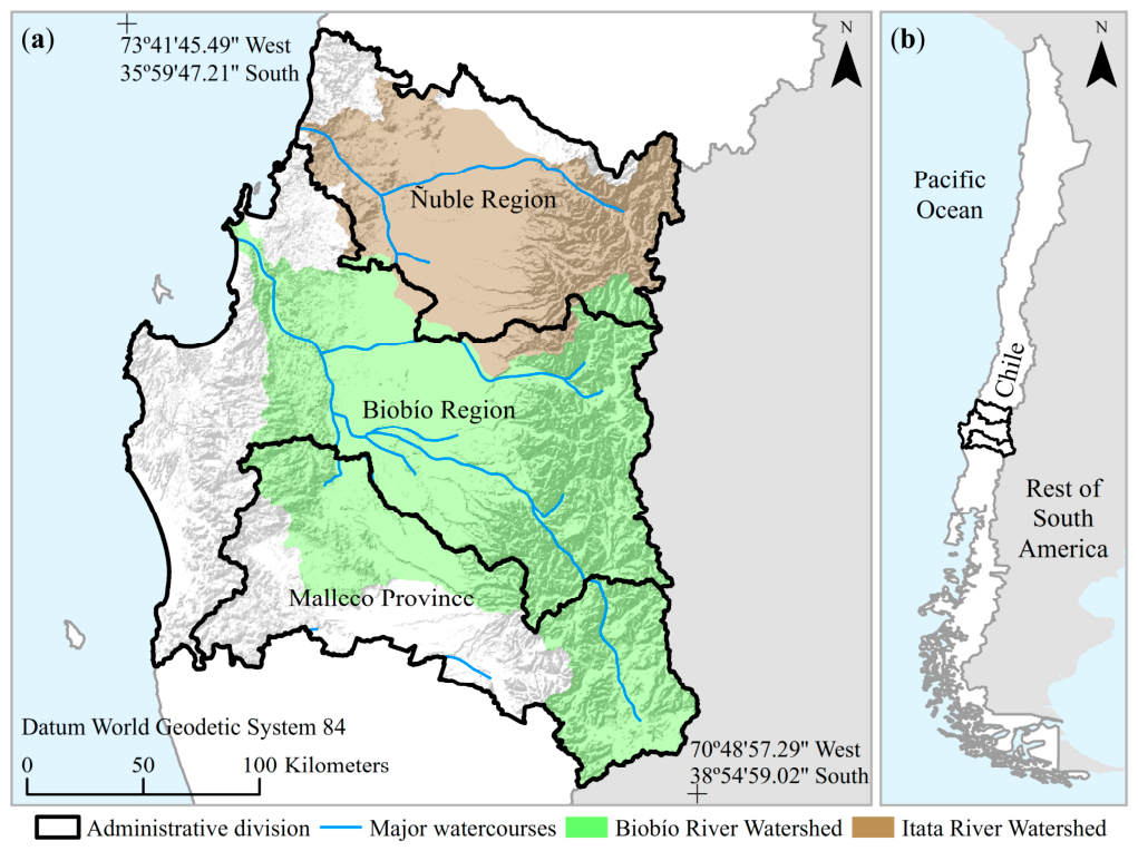
Figure 1. Study area. (a) Administrative and watershed boundaries; (b) Location in Chile.
Remotesensing 18 02969 g001
Figure 2. Methods workflow. (a) Predictor processing; (b) Reference-data processing; (c) Random Forest (RF) classification and evaluation. Obs = observation-percentage axis (12.5, 25, 50, 100); Bal = color-balancing axis (No, Yes = unbalanced, balanced); Var = predictor-set axis (B = bands, BI = B + indices, BIT = BI + territorial variables); LC = land cover; κ = kappa statistic; Q50 = median; WCVκA = weighted coefficient of variation by κ averaged; LU = land use.
Remotesensing 18 02969 g002
Figure 3. Temporal stability of normalized spectral predictors by season and balancing treatment. (a) Standard deviation (SD) of period averages; (b) SD of period-level SDs. Lower values indicate greater stability. Bands: B b , B g , B r = blue, green, red; B n i r = near-infrared; B s w i r 1 , B s w i r 2 = shortwave-infrared 1, 2; B b t = brightness-temperature. Indices: E v i , G c i , S i p i = enhanced vegetation, green chlorophyll, structure-insensitive pigment; B s i , N b r i , N d w i = bare soil, burned ratio, difference water. Period-level band distributions are shown in Figure A4 (Appendix B.1).
Remotesensing 18 02969 g003
Figure 4. Sample imbalance in period-averaged classified area and observation frequencies across sample stages. Metrics are the coefficient of variation (CV, %) and maximum-to-minimum ratio as labels. Observation frequencies average four random-seed versions before subsampling; lower values indicate greater balance. The y-axis shows pooled and unpooled LC categories (a–d) and periods (e,f). LC = land cover; C1.10 = riverbank and shore; C1.12 = without vegetation; C0.16–C0.19 = water-related classes; C0.22–C0.27 = industrial-mining and without-vegetation classes; P1 = 1997–1998.
Remotesensing 18 02969 g004
Figure 5. Relationship between validation-WCVκA and validation-κ Q50 for grouped, combined grouped, and ungrouped treatments. Q50 = median; WCVκA = weighted coefficient of variation by κ averaged; Orange, Yellow, Green = low-, moderate-, high-performance zones. Higher Q50 and lower WCVκA indicate better performance and RF-configuration convergence. Treatments: Obs-Bal-Var; Obs = observation %; Bal = color balancing (No, Yes = unbalanced, balanced); Var = predictor set (B = bands, BI = B + indices, BIT = BI + territorial variables). R2 = coefficient of determination.
Remotesensing 18 02969 g005
Figure 6. Distributions of validation-κ by grouped treatment. (a) Obs; (b) Bal; (c) Var; (d) Obs-Bal; (e) Obs-Var. Obs = observation %; Bal = color balancing (No, Yes = unbalanced, balanced); Var = predictor set (B = bands, BI = B + indices, BIT = BI + territorial variables). * = statistical significance; Ne, S, M, L = negligible, small, moderate, large effect sizes.
Remotesensing 18 02969 g006
Figure 7. Distributions of validation-κ differences by grouped treatment. (a) Obs–Obs; (b) Bal–Bal; (c) Var–Var; (d) Obs-Bal–Obs-Bal; (e) Obs-BI–Obs-BIT. Obs = observation %; Bal = color balancing (No, Yes = unbalanced, balanced); Var = predictor set (B = bands, BI = B + indices, BIT = BI + territorial variables). Obs-B–Obs-BI comparisons are omitted for S or Ne effects. * = statistical significance; S, M, L = small, moderate, large effect sizes; negative values indicate decreases between paired levels.
Remotesensing 18 02969 g007
Figure 8. Distributions of validation-κ for the Obs-No-BI and Obs-Yes-BIT series across observation levels. (a) Validation-κ values; (b) Validation-κ differences. Obs = observation %; No, Yes = color-unbalanced, -balanced; BI = bands + indices; BIT = BI + territorial variables. * = statistical significance; M, L = moderate, large effect sizes.
Remotesensing 18 02969 g008
Figure 9. Relative predictor importance based on RF mean decrease impurity by treatment. (a) 100-Yes-B; (b) 100-Yes-BI; (c) 100-Yes-BIT. Higher values indicate greater within-treatment importance; error bars show standard deviation across six replications. 100 = 100% observations; Yes = color-balanced; B = bands; BI = B + indices; BIT = BI + territorial variables. Variable codes follow Table 2.
Remotesensing 18 02969 g009
Figure 10. Rectangular representation of the 100 largest LU transitions, ordered by area. Rectangle area is proportional to transition area. The first seven columns show unchanged across P1–P12 (57.1% of the study area); remaining columns show intermediate transition pathways.
Remotesensing 18 02969 g010
Figure 11. Annual exponential LU-change rates by category and study-period group. C2.1 = agricultural; C2.3 = scrubland; C2.4 = forest plantation; C2.5 = native forest. (a) Literature-derived, 1975–2001 (centered on 1991.3); (b) Literature-derived, 1997–2020 (centered on 2008.2); (c) This study. Avg = average midpoint year. Supporting information is reported in Table A17 (Appendix B.3).
Remotesensing 18 02969 g011
Table 1. Landsat image availability and potential captures by period, season, and maximum-cloudiness threshold.
Period or
Statistic
Landsat
Satellites
Overpasses per
Season
Captures per
Season
Winter
10%
Winter
75%
Winter
100%
Summer
10%
Summer
75%
Summer
100%
Winter
Capture
Rate (%)
Summer Capture Rate (%)
P1 1997–1998 †5232061435404577831940
P2 1999–20005, 7343082974881171681752957
P3 2001–20025, 734308341251531111681835059
P4 2003–20045, 7 ‡34308411121321602582654386
P5 2005–20065, 7 ‡34308391571721332082185671
P6 2007–20085, 7 ‡34308571251361752372434479
P7 2009–20105, 7 ‡343083486981182012173270
P8 2011–20125 §, 7 ‡, 8 §343084197103881511563351
P9 2013–20147 ‡, 834308622032352102842947695
P10 2015–20167 ‡, 834308481772251642682847392
P11 2017–20187 ‡, 834308671842171712612807091
P12 2019–20207 ‡, 834308671762061712652816791
Total 400359753315501805166325452679592882
† = more extended period; ‡ = L7 scan-line gaps; § = few images. P8 assumes two satellites because L7 was fully available and L5 and L8 operated partially. Overpasses = estimated acquisition dates under 16-day repeat cycle; Captures = estimated scene captures assuming nine scenes per overpass; Capture rate = images at 100% cloudiness/Captures; L5, L7, L8 = Landsat 5, 7, 8.
Table 2. Independent variables.
Winter BandSummer BandWinter IndexSummer IndexTerritorial
B b _ W i n B b _ S u m E v i _ W i n E v i _ S u m A s p e c t E
B g _ W i n B g _ S u m G c i _ W i n G c i _ S u m A s p e c t N
B r _ W i n B r _ S u m S i p i _ W i n S i p i _ S u m C h i l
B n i r _ W i n B n i r _ S u m B s i _ W i n B s i _ S u m M t p i
B s w i r 1 _ W i n B s w i r 1 _ S u m N b r i _ W i n N b r i _ S u m P r e p 06
B s w i r 2 _ W i n B s w i r 2 _ S u m N d w i _ W i n N d w i _ S u m T e m p 02
B b t _ W i n B b t _ S u m W b I n d
A c c e s C i t y
Bands: B b , B g , B r = blue, green, red; B n i r = near-infrared; B s w i r 1 , B s w i r 2 = shortwave-infrared 1, 2; B b t = brightness-temperature. Indices: E v i , G c i , S i p i = enhanced vegetation, green chlorophyll, structure-insensitive pigment; B s i , N b r i , N d w i = bare soil, burned ratio, difference water. W i n , S u m = winter, summer. A s p e c t E , A s p e c t N = east-, north-aspects; C h i l = continuous heat-insolation load; M t p i = multi-scale topographic position; P r e p 06 = June precipitation; T e m p 02 = February temperature; W b I n d = water-body index; A c c e s C i t y = city accessibility.
Table 3. Training and validation point counts by observation level and summary group.
GroupItems12.5%
Train
12.5%
Validate
25%
Train
25%
Validate
50%
Train
50%
Validate
100%
Train
100%
Validate
(a) Total188644318829413621181172663632
(b) Periods11814017186329165661330
(c) Pooled LC categories12743715778302151606303
(d) Pooled LC categories–periods1327314727145528
LC = land cover; Train = training points; Validate = validation points.
Table 4. RF-hyperparameter statistics above the 99th percentile of validation-κ within the Obs-No-BI and Obs-Yes-BIT series.
ObsBalVarBag FractionNumber of TreesVariables per SplitAvg
CV
MinQ50MaxOptCVMinQ50MaxOptCVMinQ50MaxOptCV
12.5NoBI0.551.001.001.0020100163300100306182424441631
25NoBI0.750.901.000.90101252383001502669188341623
50NoBI0.800.900.950.904125225300225232342341620
100NoBI0.800.830.950.807125175225225184686301418
12.5YesBIT0.800.900.950.808100225300225288121212141617
25YesBIT0.850.950.950.95412525030030023810148181615
50YesBIT0.850.900.950.9531502503003001914162014171613
100YesBIT0.850.950.950.9041002503002503314182018111516
Obs = observation %; Bal = color balancing (No, Yes = unbalanced, balanced); Var = predictor set (BI = bands + indices, BIT = BI + territorial variables); Min = minimum; Q50 = median; Max = maximum; Opt = optimal value; CV = coefficient of variation (%); Nº = selected configurations; Avg CV = average across the three hyperparameters (%). Lower CV indicates greater convergence.
Table 5. LU area, persistence, transitions, and annual change under first-to-last (P1, P12) and all-period (P1, ···, P12) criteria.
C2P1P12(P1
+ P12)
⁄2
(P1 + ···
+ P12)
⁄12
(d)
− (e)
Un-changed
(P1, P12)
Un-changed
(P1, ···, P12)
(g)
− (h)
P1
− (g)
P12
− (g)
P12
− P1
Rate
(P1, P12)
Rate
(P1,···, P12)
(m)
− (n)
Log-trend R2
(P1,···, P12)
(a)(b)(c)(d)(e)(f)(g)(h)(i)(j)(k)(l)(m)(n)(o)(p)
C2.127.725.226.526.30.220.716.24.67.04.5−2.5−0.43−0.570.140.90
C2.21.21.41.31.4−0.11.00.80.20.20.40.20.710.620.090.44
C2.39.29.19.19.2−0.16.95.71.22.32.2−0.1−0.07−0.130.060.38
C2.432.235.133.633.9−0.325.713.412.36.69.42.90.390.52−0.130.77
C2.519.318.919.118.80.315.612.33.33.73.3−0.4−0.10−0.07−0.030.04
C2.62.11.82.02.00.01.51.30.20.60.4−0.3−0.62−0.740.110.91
C2.78.28.48.38.30.07.77.50.20.50.70.30.140.100.040.70
Total100.0100.0100.0100.00.079.057.122.021.021.00.00.000.000.000.00
(a) = code 2 (C2.1 = agricultural, C2.2 = natural meadow, C2.3 = scrubland, C2.4 = forest plantation, C2.5 = native forest, C2.6 = wetland, C2.7 = without vegetation); (bc) = P1, P12 areas; (df) = temporal averages, difference; (gi) = unchanged areas, difference; (jl) = loss, gain, net change; (mo) = annual exponential change rates; (p) coefficient of determination. Values are % of the study area, except rates (% year−1, base e ) and R2. Higher/lower R2 shows more/less consistent trend.
Disclaimer/Publisher’s Note: The statements, opinions and data contained in all publications are solely those of the individual author(s) and contributor(s) and not of MDPI and/or the editor(s). MDPI and/or the editor(s) disclaim responsibility for any injury to people or property resulting from any ideas, methods, instructions or products referred to in the content.