Article

Geospatial Foundation Models Improve Atoll Island Ecosystem Mapping: A Case Study Using AlphaEarth Embeddings


1
College of Science and Engineering, James Cook University, Douglas, QLD 4814, Australia
2
Ministry of Tourism and Environment, Malé 20096, Maldives
*
Author to whom correspondence should be addressed.
Remote Sens. 2026, 18(17), 2964; https://doi.org/10.3390/rs18172964
Submission received: 15 June 2026 / Revised: 14 August 2026 / Accepted: 26 August 2026 / Published: 2 September 2026
(This article belongs to the Section AI Remote Sensing)

Highlights

What are the main findings?
  • The use of AlphaEarth embeddings as predictor layers in spatial models improves ecosystem mapping in atoll islands for the majority of ecosystem classes found in the Maldives compared to the use of single-date Sentinel-2 satellite data alone.
  • Annual Croplands are mapped to a particularly high accuracy using AlphaEarth embeddings (user’s accuracy = 86.36%; producer’s accuracy = 65.52%) compared to using Sentinel-2 data (user’s accuracy = 36.36%; producer’s accuracy = 25.00%)
What are the implications of the main findings?
  • Ecosystem mapping will likely become more accessible, repeatable, and accurate into the future as embedding-based remote sensing spatial models continue to advance.
  • We recommend that the scale of satellite embedding production be expanded further into marine environments and that their performance be further tested.

Abstract

Ecosystems and the services they provide are essential for life but continue to undergo degradation worldwide. Satellite remote sensing has been essential for environmental mapping for decades, but can suffer poor accuracy when applied to mapping terrestrial ecosystems. Geospatial Foundation Models (GeoFMs) integrate diverse spatial data, including image data, spatial context, and temporal dynamics, and output readily available covariates called embeddings. GeoFM embeddings likely possess an improved ability to detect ecosystems over traditional approaches. In this study, we investigate whether the use of embeddings from Google’s AlphaEarth Foundations model yields improvements to ecosystem maps developed in the Republic of Maldives compared to single-date Sentinel-2 satellite imagery. We compare (1) per-class accuracies, (2) the effect of decreasing numbers of map classes on overall accuracy, and (3) the relationships between confidence, accuracy, and the number of training samples for each class. AlphaEarth outperforms Sentinel-2 (1) for individual ecosystems, (2) with increasing numbers of classes, and (3) with fewer training data samples while also being more confident in its classifications. We expect that these advantages will promote rapid uptake and expansion in the use of GeoFMs to address challenging spatial analyses, such as mapping global ecosystems and landscapes with limited available data.

1. Introduction

Ecosystems regulate climate [1], store carbon [2], control floods [3], and provide critical natural resources that underpin human wellbeing and livelihoods worldwide [4]. Ecosystems are commonly defined according to their biota and the specific interactions and dynamics of biotic assemblages, abiotic conditions, and the functional processes that link them [5,6]. Together, these characteristics influence ecosystem structure, resilience, and the services they provide. Knowledge of the spatial distributions and conditions of specifically defined ecosystems is therefore central to environmental management and conservation planning.
Despite their importance, ecosystems are degrading globally at unprecedented rates. Severe degradation has been documented across forests [7], mangroves [8], grasslands and savannahs [9], polar ecosystems [10], wetlands [11], coral reefs [12], and kelp forests [13]. Drivers of this widespread degradation are typically reported as climate change [14], land-use change [15], pollution [16], and invasive species [17], but are also compounded by direct anthropogenic stressors such as disturbance [18], overexploitation [19,20], and habitat modification [21]. In some cases, ecosystem degradation poses an existential risk to the communities that depend directly on ecosystem services, such as the over 700,000 people living on low-lying atoll islands globally [22]. Despite extensive evidence of global ecosystem decline, our ability to map and describe ecosystem distributions remains limited, constraining efforts to monitor change and guide effective conservation and restoration actions.
Satellite remote sensing, for example from the Sentinel-2 and Landsat satellites [23,24], has become a cornerstone of broad-scale environmental monitoring over recent decades, enabling repeated observations of the Earth’s surface and supporting analyses of, for example, deforestation [25], urban expansion [21], natural disasters [26], and glacial retreat [27]. Remote sensing has been widely applied to ecosystem-related studies, including assessments of tidal wetlands [28], mangroves [8], coral reefs [29], agricultural plantations [30], and land use and land cover [31]. However, the majority of satellite sensors typically focus on collecting data on electromagnetic reflectance and topography, which can then be used to infer important ecosystem properties such as vegetation abundance [32]. Different ecosystems can exhibit similar spectral signatures, limiting the ability of classification analyses to distinguish between different ecosystem types. For example, plantations and natural forests may appear similar in satellite imagery while performing fundamentally different ecological functions [30]. Additionally, training datasets developed for spatial modelling of ecosystem distributions are often sparse or unevenly distributed across classes or space, due to logistical, financial, or geographic constraints, further limiting the performance and repeatability of analytical approaches.
Recent advances in artificial intelligence (AI) offer new opportunities to address these challenges by integrating diverse spatial data sources and learning complex, non-linear patterns that can be difficult to capture using traditional methods. Deep-learning models can extract hierarchical representations of spatial information by analysing data across multiple spatial and temporal scales. Foundation Models, which are pre-trained on very large and heterogeneous datasets, have demonstrated strong performance in classification tasks even with limited task-specific training data [33]. When applied to spatially referenced data, Geospatial Foundation Models (GeoFMs), such as Google’s recently published AlphaEarth Foundations, incorporate information from a diverse range of sources, including satellite imagery, topography, climate data, species records, and other georeferenced sources of information [34]. The GeoFM learns an internal representation of these multiple input sources, and feature vectors are surfaced as an embedding dataset. These embeddings are rich representations of the Earth’s surface that overcome classical limitations in the number of spatial datasets that can effectively be used in a geospatial classification model [35,36]. Importantly, these embeddings do not require expertise or advanced understanding of satellite imagery to use, and can be loaded as easily as loading a single-date Sentinel-2 image. Thus, geospatial embedding datasets have the potential to improve ecosystem mapping by enabling straightforward access to a wealth of data from a vast array of relevant geospatial information sources. However, they may be limited in the transferability of the data they are trained on, for example in their application to marine ecosystems.
Here, we investigate whether the use of learned geospatial embeddings can improve terrestrial and shallow-marine ecosystem mapping relative to a simple traditional remote sensing approach, using an atoll archipelago, the Republic of Maldives (hereafter, the Maldives), as a case study. Atoll islands are formed from the deposition of coral-derived sediments on carbonate structures that have grown around the rims of subsiding oceanic volcanoes [37,38]. Atoll islands are typically low-lying, with maximum elevations often less than one metre above sea level, making them highly vulnerable to sea level rise. Although projections of sea level rise exceeding two metres by 2100 [39,40] raise concerns about total land loss on atoll islands [41], these features are dynamic systems that are known to respond to physical drivers of change through complex interactions between ecosystems and physical island-forming processes [42,43]. The persistence of these dynamics depends on the continued functioning of natural atoll ecosystems. However, accelerating sea level rise [44], declining coral reef accretion rates [12], and increasing human modification [45] threaten to compromise these processes into the future.
We compared the performance of embeddings generated by Google’s AlphaEarth Foundations model with that of single-date Sentinel-2 satellite imagery for mapping ecosystems across marine, terrestrial, freshwater, and transitional realms in the Maldives. Specifically, we aimed to:
  • Compare the accuracy of ecosystem maps produced using AlphaEarth Foundations embeddings and Sentinel-2 satellite imagery for randomly selected case study islands.
  • Investigate the effect of the number of ecosystem classes on overall accuracies of AlphaEarth-based and Sentinel-2-based classifications by merging classes incrementally.
  • Investigate the relationships between classification confidence, accuracy and the number of training samples for each ecosystem class between the AlphaEarth-based and Sentinel-2-based classifications.

2. Materials and Methods

2.1. Study Sites

The Maldives is an archipelagic chain of ~1192 low-lying islands [46] distributed over 20 administrative atolls and located around a central point of 3.2028°N, 73.2207°E [47]. The Maldives is ~870 km in length and ~128 km in width with a maximum natural height of 2.4 m above mean sea level [46]. It has a total land surface area of ~160 km2 [48] but a total marine sovereignty of ~922,000 km2 [49]. The country supports a population of 526,000 people as of 2023 [22]. The main sources of income in 2016 were tourism (30%), agriculture (1.6%), and fisheries (1.3%) [46]. There is a strong monsoonal cycle, with two monsoons per year [46]. The main forces shaping the geography and climate are oceanic, with strong seasonally reversing winds and large waves [50], with these waves being dissipated at the reef crest and directing sediment to form islands [43]. As a low-lying oceanic atoll nation, the Maldives is particularly vulnerable to tsunamis [51] and sea level rise [46].
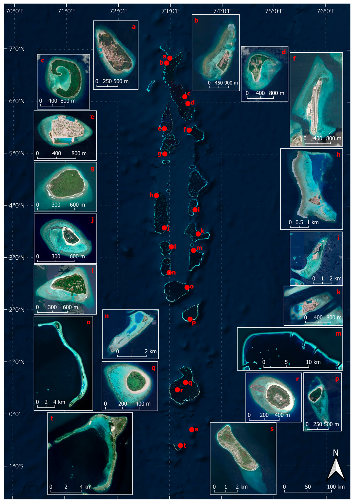
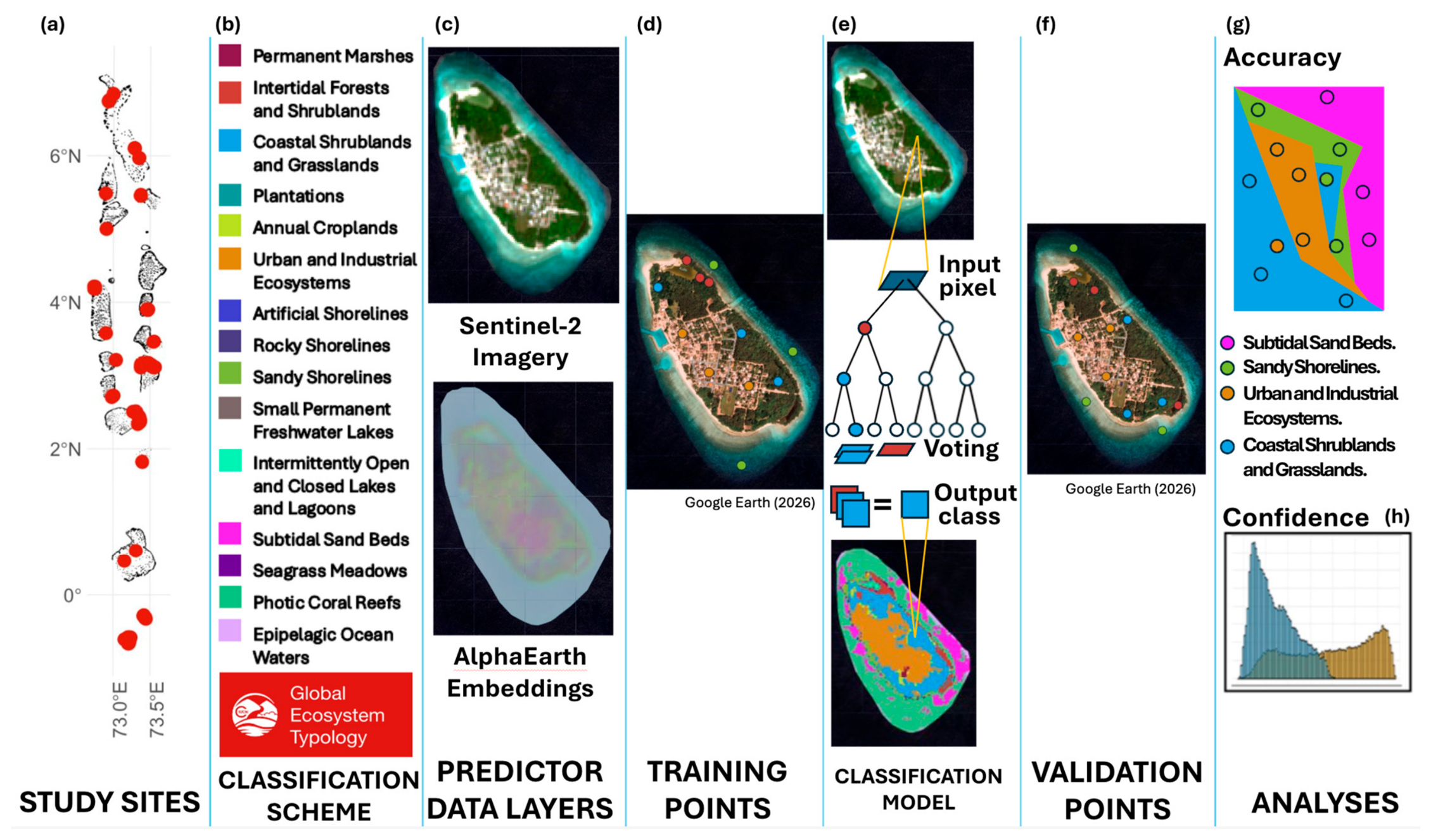
We selected 20 sites across the country, with each site representing each of the 20 administrative atoll divisions officially recognised by the Government of Maldives (Figure 1 and Figure 2a; Table A1). The stratification by administrative atoll served to maximise representation of conditions observed across the Maldives. Large differences in latitude may influence the distribution of ecosystems via its effect on, for example, climatic, socioeconomic, or oceanographic conditions. Before filtering, 2573 reefs were available as candidates. Study sites were selected at the unit of reef platforms and, to ensure that each site possessed adequately large instances of marine and terrestrial ecosystems, only those reef platforms with islands larger than five ha were considered for selection. In addition, to prevent any one single island dominating the spatial analysis, we applied a maximum threshold reef platform size of 5000 ha. These thresholds were attained through informal trial and error to ensure that they only removed extreme cases of site geomorphology. After this filtering, 404 reefs were available as candidates, of which we picked one randomly on each administrative atoll using a random seed. Data representing island coastlines and reef extents were acquired from www.onemap.mv (accessed on 15 April 2025), a map product authorised and managed by the Maldivian government.

2.2. Ecosystem Classification Scheme

Our focus was to develop a map of ecosystems, and we opted to use the current global standard classification scheme for ecosystems, the International Union for Conservation of Nature (IUCN) Global Ecosystem Typology (GET) [5,6]. Previous work in the Maldives [52] identified 33 present, or potential, ecosystem functional groups (hereafter referred to as ‘ecosystems’) (Table 1). From this candidate set we excluded ecosystems that were suspected but not confirmed in the Maldives or that are impossible to identify from satellite imagery: Coastal Saltmarshes and Reedbeds (IUCN code MFT1.3), Muddy Shorelines (MT1.2), all aphotic ocean ecosystems, and subterranean ecosystems. Oceanic areas in which the ocean floor could not be directly observed in satellite imagery (i.e., deeper than ~20 m) were classified as Epipelagic Ocean Waters (Deep Water) (M2.1). Lastly, we merged Subtidal Rocky Reefs (M1.6) with Photic Coral Reefs (M1.3) due to difficulties differentiating these two ecosystems during image interpretation (see Section 2.4). The final classification scheme for this study therefore included 15 ecosystems, of which nine were predominantly terrestrial and six were aquatic (Figure 2c, Table 1).

2.3. Predictor Data Layers

In remote sensing classification analyses, predictor data layers that comprehensively cover the region of interest are required to enable comprehensive spatial predictions of each map class. The two sources of predictor data used in this analysis are Sentinel-2 satellite imagery [24] and embeddings from Google’s AlphaEarth Foundations model [36] (Figure 2b).
The Sentinel-2 mission currently operates a set of two Earth observation satellites as part of the European Space Agency’s Copernicus programme. On each satellite is a MultiSpectral Imager (MSI) sensor that records reflected electromagnetic radiation from the Earth’s surface in 13 spectral bands. The Sentinel-2 satellites have a swath width of 290 km and a revisit time of five days, and deliver satellite images with a minimum 10 m pixel resolution. As predictor data layers, we used data values from Sentinel-2 data bands 2 through to 12, excluding 9 and 10, and layers processed to Normalised Difference Water Index (NDWI) and Normalised Difference Vegetation Index (NDVI). NDWI and NDVI are widely used indices that exploit the consistent, known differences in reflection between green and near-infrared radiation from water (NDWI) [53] and red and near-infrared radiation from vegetation (NDVI) [32]:
N D W I   =   G   −   N I R G   +   N I R
N D V I   =   N I R   −   R N I R   +   R
where G = green radiation (Sentinel-2 MSI band 3), NIR = near-infrared radiation (Sentinel-2 MSI band 8), and R = red radiation (Sentinel-2 MSI band 4). We filtered the Sentinel-2 Level 2 image collection for all images acquired that intersected our 20 study sites between 1 January 2023 and 29 September 2025. The most cloud-free image was selected for each study area and the images were stitched together into a single mosaic. The dates acquired for each study island can be found in Table A1. A mosaic of images from multiple different dates was necessary due to the high cloud cover commonly present in the Maldives. Different conditions between sites are not deemed an issue as temporal trends and processes are written into the ecosystem definitions (for example, Sandy Shorelines are defined as being shaped predominantly by intertidal action and Annual Croplands are defined by their annual cycle of harvest and regrowth).
AlphaEarth embeddings are analysis-ready outputs from Google’s AlphaEarth Foundations model [36]. The data inputs into the AlphaEarth embedding model includes satellite optical (from the Sentinel-2 and Landsat 8/9 satellite image archives), radar (from the Sentinel-1 and PALSAR2 satellites), LiDAR (from the GEDI satellite), environmental (from the GLO-30, ERA5-Land, and GRACE models), labelled land cover datasets (USGS National Land Cover Database [54] and United States Department of Agriculture Cropland Data Layer [55]), and geospatial text data (Wikipedia and the Global Biodiversity Information Facility [36,56]). These data are collected over multiple time periods and used to develop annual time-series embedding outputs. Thus, each annual AlphaEarth embedding layer represents a full year of information and is therefore useful for integrating temporal dynamics into data layers suitable for use in spatial models, such as crop harvesting cycles or deciduous phenology of ecosystems. In addition, AlphaEarth embeddings include kernels for each pixel that enable pixel values to be influenced by information from around that pixel, enabling representation of some spatial context at the pixel scale. The result of the GeoFM is a 64-dimensional, information rich set of satellite embedding data layers at 10 m spatial resolution with global coverage which can be analysed in the same way as standard satellite data [36]. As recommended by [36], we use all 64 embedding data bands in our analysis. AlphaEarth embeddings covering the year 2023 were used in this analysis.

2.4. Sampling and Annotating Training Points

To train a classification model to estimate class membership of pixels within each study site, we developed a set of training data points to represent occurrences of the 15 ecosystems addressed in this study. We developed a stratified random sample of 1000 training data points across the study sites, limiting our sampling to the selected site polygons expanded by a standard 10 m buffer to ensure the inclusion of the deep-water class (see above). As the areal extent of reefs (10,900 ha) in the Maldives exceeds that of islands (1660 ha), we employed stratified sampling over areas of land and water with a ratio of 60:40 (according to the proportion of land-based ecosystems (nine) to aquatic ecosystems (six)) to ensure adequate sample size over land areas. To achieve this stratification, we developed land and water masks using the NDWI calculated with Sentinel-2 MSI data. During annotation, additional points were sampled interactively to ensure representations of rare ecosystems, such as Rocky Shorelines (MT1.1), Intermittently Open and Closed Lakes and Lagoons (FM1.3), and Plantations (T7.3) that may not have been adequately sampled during the random stratified sampling procedure. Interactive points were opportunistically gathered and focused on ecosystems deemed insufficiently sampled after the first round of annotation. The search area for the interactive points was based around the initial, randomly sampled points and so they were effectively randomly distributed across the islands. A total of 201 interactive points were gathered, yielding a total of 1201 points for annotation.
Annotation (i.e., labelling) of each point with its most-likely ecosystem type was conducted according to the most recent cloud-free Sentinel-2 satellite imagery by a single trained interpreter (G.L.). For points at which the ecosystem type was not clear from the Sentinel-2 satellite imagery, additional sources of information were employed to aid interpretation, including time-series of very-high-resolution MAXAR satellite imagery accessed through Google Earth Pro between the years 2004 and 2025 [47], relevant publicly available geospatial datasets (e.g., the Allen Coral Atlas [29]) and, opportunistically, using information from Google Street View and publicly uploaded images on Google Maps. For the island of Fuvahmulah, a map developed from high-resolution drone imagery was provided by the fifth author that allowed image interpretation and calibration of each class among the different information sources. The drone map was especially useful for Annual Croplands, an ecosystem which is concentrated largely in Fuvahmulah across our study sites and which are difficult to annotate from satellite imagery due to their small scale and frequent interspersion with other classes. Each training point was a 10 × 10 m square, and labels collected included dominant ecosystem, homogeneity (recorded as the percentage cover of the dominant ecosystem within each square), and a confidence score collected on a scale of 1–5 from lowest to highest confidence. Points were reviewed once after the initial round of annotation. Once the full set of 1201 points were annotated with their most-likely dominant ecosystem, they were filtered to remove points with a homogeneity of less than 60% and a confidence of less than 4. The final training dataset then consisted of 902 points (Figure 2d, Table 1).

2.5. Classification Model

Two Random Forest classifiers were trained with one set of predictor layers each (Sentinel-2 bands/indices or AlphaEarth embeddings) and the same set of training and validation points. Random Forest is a machine learning algorithm that uses multiple, deep decision trees to reach a consensus on pixel classification [57]. Due to its ability to handle complex and highly correlated input data, Random Forest is a commonly employed model in remote sensing analyses [57,58]. In this study, a Random Forest with 500 trees was employed to estimate the ecosystem class that each pixel belongs to within the study area (Figure 2e). This number was chosen to maximise accuracy as the analysis was run remotely in Google Earth Engine and so there was minimal computational limitation [59]. Aside from the number of trees, default parameters were employed. The square root of the number of covariates were allowed for each decision node, and half the training data was sampled to grow each tree (bag fraction of 0.5). Ten more Random Forest models were run, with the same parameters, for the reduced stages developed for the class reduction analysis (see Section 2.8). Five of these ten models employed the 64 AlphaEarth embedding data layers as predictors, while the other five employed the Sentinel-2 data bands and indices as predictors. For purposes of readability, the maps produced will hereafter be referred to according to the predictor layers used to create them, ‘AlphaEarth’ and ‘Sentinel-2’.

2.6. Sampling and Annotating Validation Points

To support validation of our ecosystem map outputs, we developed an independent set of annotated validation points. The strong variation in extent of each ecosystem posed an issue here, as a simple random sample would produce a heavy skew towards more common ecosystems (as noted in Section 2.4). To address this issue, we developed and combined three sets of sample points to aim for at least 20 unbiased validation points to be acquired for each ecosystem as follows.
The initial sample set was 280 randomly distributed points, split 60:40 between land and water (as described in Section 2.4). These points were overlaid on a preliminary map of ecosystems developed using AlphaEarth embeddings and assessed for class balance. To supplement samples for rare ecosystems, we generated a minimum of 20 randomly sampled validation points per ecosystem using an oversampling procedure. A total of 5000 points were randomly sampled across all study sites, intersected with the preliminary map and randomly reduced until each ecosystem was represented by a minimum of 20 points. Once this was achieved, the second sample was combined with the first sample: points from the first sample were kept if they belonged to an ecosystem that was represented by more than 20 points in the first sample, and points from the second sample were kept if they belonged to an ecosystem that was represented by less than 20 points in the first sample. This created a semi-final sample set with a minimum of 20 points per ecosystem, with proportionally more points for ecosystems with greater area. To remove potential bias towards AlphaEarth, a second oversampling procedure was conducted according to a preliminary Sentinel-2 map, adding an additional 260 points to the validation set, which were filtered down to an additional 206 points as some were within 1 metre of other points. The validation set was then sorted by longitude to shuffle the sample set for interpretation and annotated to the pinpoint according to MAXAR imagery. Each sample was annotated with the same fields as the training data, and all points with a confidence < 2 were removed. The different threshold for inclusion was chosen as there were fewer validation points. Owing to a lack of suitable occurrences, Intermittently Open and Closed Lakes and Lagoons (FM1.3) were removed from subsequent analyses. The final validation dataset consisted of 545 points over the 14 classes, though unfortunately several rare ecosystems were ultimately represented by less than 20 points each (Figure 2f, Table 1). Rocky Shorelines, for example, are extremely rare in the Maldives. Beaches with large pieces of coral rubble are defined as Sandy Shorelines under the IUCN GET.

2.7. Per-Class Accuracy

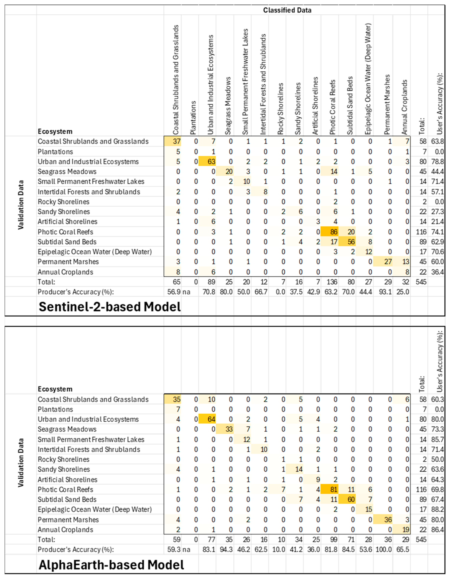
To comparatively assess the accuracy of the classified maps produced from the 12 models, the validation dataset was used to calculate a range of standard accuracy assessment metrics. Confusion matrices were used to calculate user’s accuracy (UA) and producer’s accuracy (PA) per map [60], along with F-1 scores and area-adjusted UAs and PAs.
UAs and PAs are calculated as functions of the number of correctly classified points against the total number of points either classified to a class or that are labelled within the validation point set:
U A   =   n i i n + i   ×   100
P A   =   n i i n i +   ×   100
where nii = the number of points correctly classified in a class, n+i = the total number of validation points in the class, and ni+ = the total number of points classified to the class in the model. F-1 scores are calculated as a function of UA and PA:
F 1   =   2   ×   U A × P A U A + P A
Finally, area-adjusted accuracies require the calculation of area weights:
W i = A i A T
where Wi = area weight, Ai = the area of the ecosystem (per model), AT = the total area of ecosystems (per model). Then, adjusted cell proportions are calculated:
p i j   =   W i   ×   n i j n i +
where pij = adjusted cell proportion at cell position i, j. Area-adjusted UAs and PAs are then calculated in much the same way as normal UA and PA:
A r e a   a d j u s t e d   U A =   p i i ∑ j p j i
A r e a   a d j u s t e d   P A = p i i ∑ j p i j
Overall accuracy, which was used to investigate the impact of class reduction on map accuracies, was calculated as the proportion of validation points with an annotated class that matches the model-classified class over the full validation dataset (Figure 2g). A McNemar’s test was employed to test for statistical differences between the performance of the two maps, and a Wilcoxon’s Signed-Rank test was employed to test for a statistical difference between the UA and PA of the two models.

2.8. Class Reduction Analysis

To investigate the effect of the number of classes on the accuracy of classification maps produced using AlphaEarth embeddings and using Sentinel-2 satellite imagery (objective two), we incrementally combined the total list of 15 ecosystems according to spectral or ecological similarity and produced six classification scenarios (I–VI) with incrementally decreasing numbers of classes (Table 2). The merging of classes between scenarios III and IV was opportunistically designed to provide insight into the capabilities of the predictor layers for mapping shallow marine ecosystems, where the only change was the merging of Subtidal Sand Beds (M1.7), Seagrass Meadows (M1.1), and Photic Coral Reefs (M1.3) into one Shallow Water Ecosystems class, and the exclusion of Small Permanent Freshwater Lakes (F2.2) and Intermittently Open and Closed Lakes and Lagoons (FM1.3) (represented by ‘NA’ in Table 2). The freshwater classes were removed here specifically to focus on shallow marine ecosystems. Overall accuracy was calculated on each scenario and a Wilcoxon signed-rank test was used to test for statistical significance between the models. Importantly, as the validation sample was not entirely random due to the applied floor for rare ecosystems, the overall accuracy acts as a sample-level comparison. This better represents performance on the variety of ecosystems present and reduces the dominance of large-area ecosystems such as Photic Coral Reefs or Urban and Industrial Ecosystems.

2.9. Confidence, Accuracy, and Training Sample Size

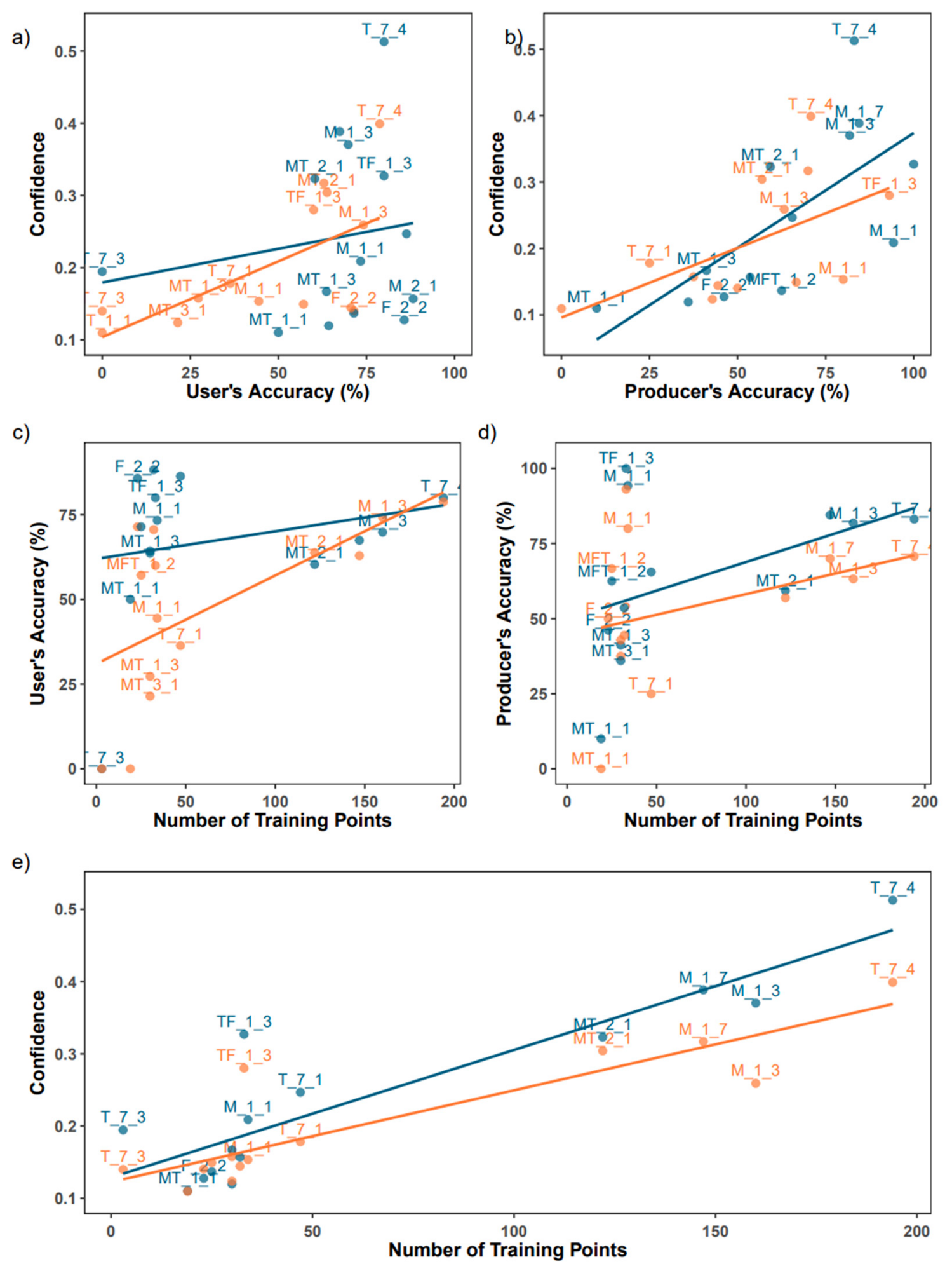
For objective 3, we intend to investigate the confidence of the classified maps. Here, the proportion of trees in the random forest that assigned a pixel to each class is referred to as a model ‘confidence’. Higher values of confidence indicate more trees agreed on the class. This term is used for simplicity as a way to communicate model reliability [61], noting that high confidence is not always synonymous with high accuracy [62] (Figure 2h). As there was variation in the extent of ecosystems and, as a consequence, the number of training points for each ecosystem, the effect of training dataset size on confidence and accuracy could be assessed. We compared (i) the confidence of each ecosystem classification against UA and PA; (ii) UA and PA against the number of training points for each ecosystem; and (iii) the confidence of each ecosystem classification against the number of training points for each ecosystem.

2.10. Landscape Metrics

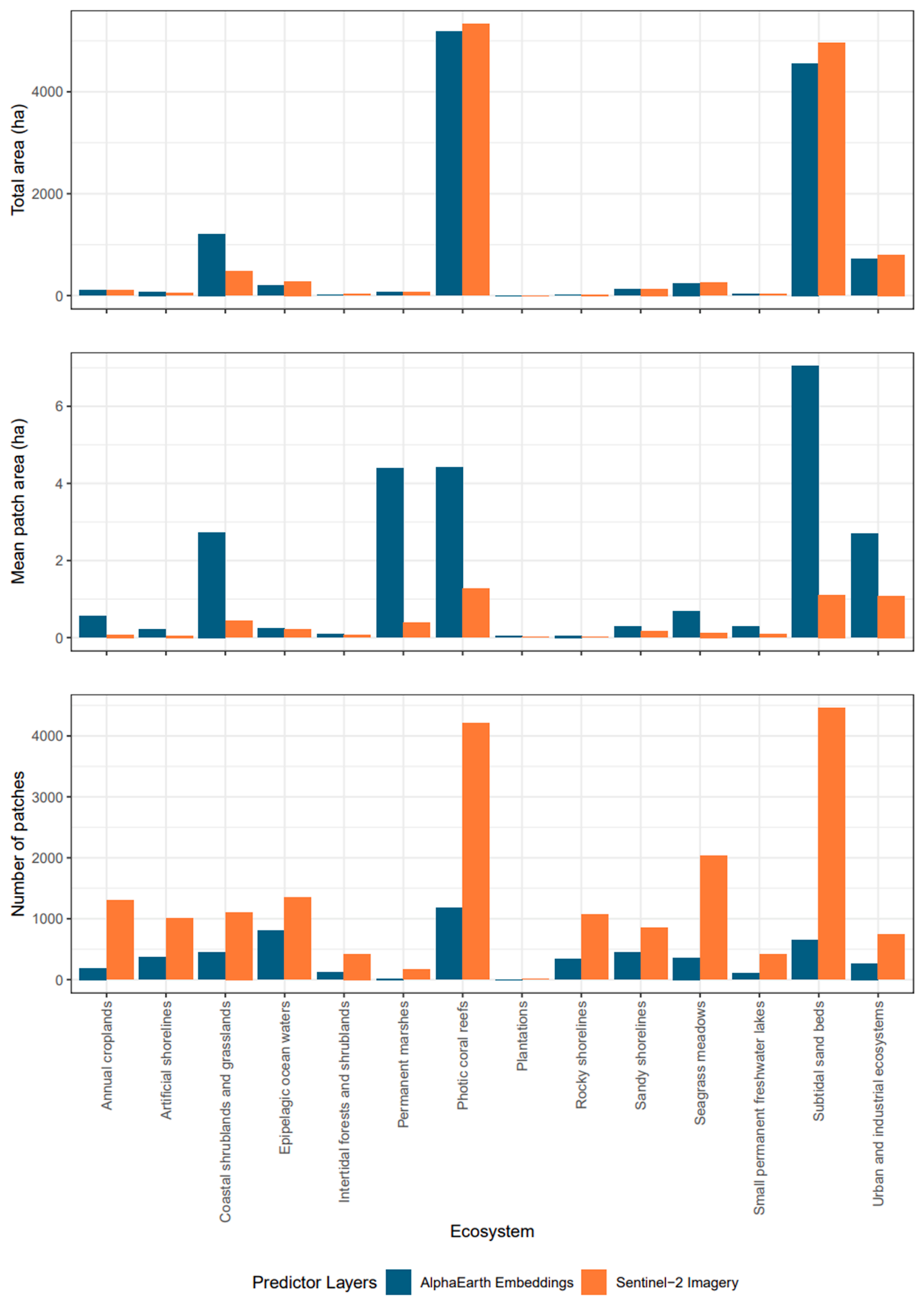
To quantify spatial differences between the Sentinel-2 and AlphaEarth predictions, we calculated three landscape metrics for each ecosystem type: total area, number of patches, and mean patch area. Patches were defined as one or more touching pixels from the same ecosystem, including touching on the diagonal.

2.11. Software

Analyses were conducted in R using Rstudio (version 1.2.418), with the packages ggplot2 (version 4.0.3), dplyr (version 1.2.1), tidyr (version 1.3.2), stringr (version 1.6.0), terra (version 1.9.46), tidyterra (version 1.3.0), ggspatial (version 1.1.10), beepr (version 2.0), scales (version 1.4.0), broom (version 1.0.13), tidyverse (version 2.0.0), sf (version 1.1.2), archive (version 1.1.14), ggrepel (version 0.9.8), gridExtra (version 2.3.1), and patchwork (version 1.3.2) (all code available in Supplementary Material) [63,64] and Microsoft Excel (2024) [65], and map generation was conducted in Google Earth Engine (version 1.7.41) [59]. Point annotation was conducted in OlmoEarth [66]. The workflow was entirely scripted for purposes of repeatability.

2.12. Generative Artificial Intelligence Statement

Generative Artificial Intelligence (GenAI) was used for support in coding and understanding complex concepts in deep-learning technology.

3. Results

3.1. Per-Class Accuracy

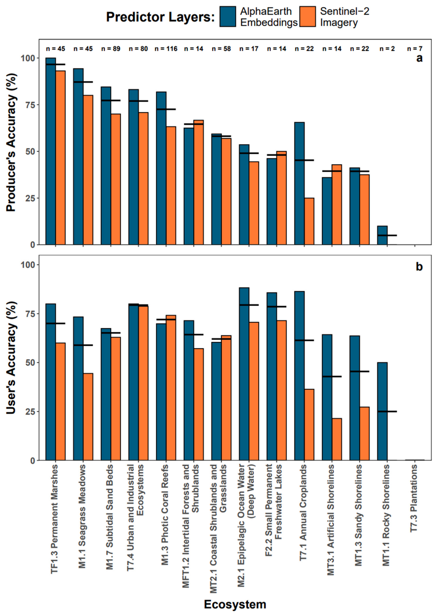
AlphaEarth achieved higher accuracies than Sentinel-2 for the majority of the 14 classes in all five accuracy metrics (UA: 11 classes; PA: 10 classes; F-1 score: 12 classes; Area-adjusted UA: 11 classes; Area-adjusted PA: 10 classes) with the greatest difference being in UA and area-adjusted UA for Annual Croplands (UAAlphaEarth = 86.36%; UASentinel-2 = 36.36%), Artificial Shorelines (UAAlphaEarth = 64.29%; UASentinel-2 = 21.43%), and Sandy Shorelines (UAAlphaEarth = 63.64%; UASentinel-2 = 27.27%). UA and area-adjusted UA are identical for all classes and both models, so we will only report UA here for purposes of readability. The smallest differences are in F-1 Score for Coastal Shrublands and Grasslands (F-1 ScoreAlphaEarth = 59.83%; F-1 ScoreSentinel-2 = 60.16%), UA and area-adjusted PA for Urban and Industrial Ecosystems (UAAlphaEarth = 80.00%; UASentinel-2 = 78.75%; area-adjusted PAAlphaEarth = 71.99%; area-adjusted PASentinel-2 = 70.91%), and in F-1 Score for Small Permanent Freshwater Lakes (F-1 ScoreAlphaEarth = 60.00%; F-1 ScoreSentinel-2 = 58.82%) (Figure 3 and Figure 4, Table 3).
The highest UA reported was 88.24% for AlphaEarth for Epipelagic Ocean Waters (Deep Water) and 78.75% for Sentinel-2 for Urban and Industrial Ecosystems. Urban and Industrial Ecosystems, Photic Coral Reefs, Permanent Marshes, Subtidal Sand Beds, and Seagrass Meadows were consistently mapped to a high accuracy between models and under different accuracy metrics (Figure 3 and Figure 4, Table 3). The highest PA reported in both models was for permanent marshes, which was 100% and 93.10% for AlphaEarth and Sentinel-2, respectively.
A McNemar’s Chi-squared test with continuity correction reveals a significant difference between the performance of the two models (NcNemar’s chi-squared = 18.395, d.f. = 1, p = 1.796 × 10⁻⁵). Similarly, two Wilcoxon signed rank exact tests reveal a significantly higher performance of AlphaEarth for PA (V = 79/91, p = 0.01709) and for UA (V = 86/91, p = 0.005169) between the two models.

3.2. Class Reduction Analysis

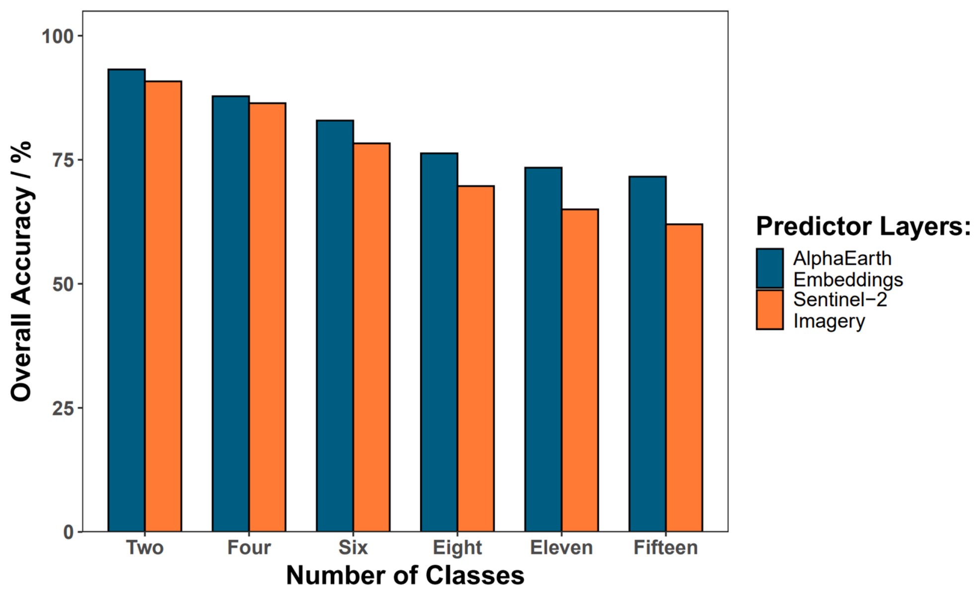
Our results indicate that overall accuracy of the ecosystem maps decreases as the number of classes increase in both AlphaEarth and Sentinel-2 (Figure 5, Table 4), with AlphaEarth consistently achieving higher accuracies than Sentinel-2 (Wilcoxon’s Signed-Rank Exact Test: V = 21/21, p = 0.03125). When the classification scheme was reduced to only two or four classes, the two models achieved similar overall accuracy (AlphaEarth: 93.2% (two classes), 87.8% (four classes); Sentinel-2: 90.8% (two classes), 86.4% (four classes). Accuracy continues to drop for both as the class numbers increase. Moving from six to eight classes results in a considerable drop in accuracy for both maps (6.7% drop for AlphaEarth and 8.7% for Sentinel-2), corresponding with the splitting of Shallow Water Ecosystems into Seagrass Meadows, Subtidal Sand Beds and Photic Coral Reefs. Following this, the difference grows larger with each increase in the number of classes. AlphaEarth drops in accuracy by 4.7% between 8 and 15 classes from 76.3 to 71.6%, but Sentinel-2 drops by 7.7% from 69.7 to 62.0% (Table 2).

3.3. Confidence, Accuracy, and Training Sample Size

AlphaEarth had a higher overall confidence, but it had a weak relationship between UA and confidence while Sentinel-2 had a positive relationship (AlphaEarth: R2 = 0.0282; Sentinel-2: R2 = 0.389) (Figure 6a). For PA against confidence, AlphaEarth had a stronger positive relationship than Sentinel-2 (AlphaEarth: R2 = 0.487; Sentinel-2: R2 = 0.316) (Figure 6b). As the number of training points increased, UA increased for Sentinel-2 (AlphaEarth: R2 = 0.0522; Sentinel-2: R2 = 0.372) (Figure 6c), while PA increased for both AlphaEarth and Sentinel-2 (AlphaEarth: R2 = 0.214; Sentinel-2: R2 = 0.121) (Figure 6d). Finally, confidence increased in a positive linear trend that was stronger for AlphaEarth than with Sentinel-2 (AlphaEarth: R2 = 0.801; Sentinel-2: R2 = 0.780) (Figure 6e).

3.4. Landscape Metrics

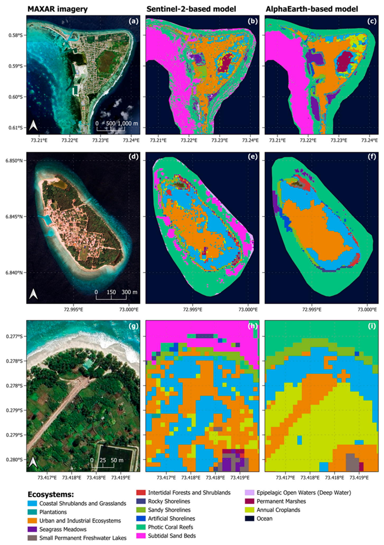
AlphaEarth produces a more spatially coherent map that appears to better represent the distribution of ecosystems in the study islands (Figure 7). AlphaEarth consistently predicted larger and fewer patches across all ecosystems compared to Sentinel-2 (Figure 8, Table 5). AlphaEarth predicted larger total areas of Coastal Shrublands and Grasslands (diff = 729.36 ha), whereas Sentinel-2 predicted larger total areas of Subtidal Sand Beds (diff = 404.69 ha), Photic Coral Reefs (149.05 ha), Epipelagic Ocean Water (Deep Water) (84.01 ha) and Urban and Industrial Ecosystems (82.10 ha) (Figure 8, Table 5). For example, the island of Hulhudhoo possesses continuous croplands in its North-East corner (Figure 7a) which is classified predominantly as Urban and Industrial Ecosystems and Coastal Shrublands and Grasslands with Sentinel-2 (Figure 7b), but as Annual Croplands with AlphaEarth (Figure 7c). Similarly, the mangroves present in the North and South-East of the island of Thakandhoo (Figure 7d) are interspersed with Permanent Marshes and Annual Croplands with Sentinel-2 (Figure 7e), but appear as smooth continuous Intertidal Forests and Shrublands features with AlphaEarth (Figure 7f). In the Northern point of Fuvahmulah, a clear separation of croplands and roads is observed (Figure 7g), which is indiscernible with Sentinel-2 (Figure 7h), but clear with AlphaEarth (Figure 7i).

4. Discussion

4.1. AlphaEarth Outperformed Sentinel-2

Our study indicates that AlphaEarth outperforms single-date Sentinel-2 imagery for ecosystem mapping in the Republic of Maldives. To our knowledge, this is the first analysis that compares the performance of a geospatial foundational model to that of a traditional image-based remote sensing classification for the task of spatially mapping ecosystems on oceanic atoll islands. We found that the majority of ecosystems in this study were mapped to a higher accuracy using AlphaEarth embeddings than using predictors derived from the Sentinel-2 satellite imagery archive. Decreases in accuracy due to increasing class complexity were also reduced with AlphaEarth compared to Sentinel-2. Finally, our results indicated that AlphaEarth, on average, increased in per-pixel classification confidence with increased size of the training dataset, though only marginally, but still achieved high accuracies even with small training datasets. These results are in agreement with other studies on AlphaEarth that find it outperforms traditional methods for mapping wetlands [67], mangroves [68], tree species [69,70], native grasslands [71], and urban air quality [72]. We are therefore confident in our result that AlphaEarth is more effective at mapping atoll ecosystems in the Maldives than Sentinel-2.

4.2. Croplands

Annual Croplands were mapped to a particularly higher accuracy with AlphaEarth (UAAlphaEarth = 86.36%; PAAlphaEarth = 65.52%) than with Sentinel-2 (UASentinel-2 = 36.36%; PASentinel-2 = 25.00%) (Figure 3, Table 3). Our results broadly correspond to studies such as [73,74], which found that cropland maps produced using AlphaEarth embeddings achieved overall accuracies in excess of 90% (91.4% and 99.1%, respectively). These cropland maps are, however, at a much larger scale than the crops considered here. While accuracies of map classifications are known to be affected by a broad range of variables such as the accuracy and amount of training data [75], class balance of the training data [76], feature size [77], and class phenology [78], we note that croplands in Maldives are typically small-scale landholder farms that occur as small-patch fields of taro, sweet potato, and eggplant, among others (Figure 7g), while refs. [73,74] consider extensive wheat, soybean, and corn crops across Japan, Europe, and the United States. Small-scale crops are known to be challenging to map accurately, especially due to difficulties identifying them from satellite imagery [79]. However, extreme care was taken differentiating cropland from other similar classes, which was aided by the high resolution drone map which covered a large portion of annual croplands present across our study sites, and we are confident in the accurate annotation of Annual Croplands in this study. Our finding that AlphaEarth achieved class accuracies for mapping small-scale croplands that exceed well published rules-of-thumb suggests it is promising for the future of monitoring these essential island ecosystems.

4.3. Shorelines

Our AlphaEarth-based model consistently achieved higher UA than Sentinel-2 for mapping shoreline ecosystems, though absolute accuracy was low (UAAlphaEarth = 50.00–64.29%; PAAlphaEarth = 10.00–41.18%; UASentinel-2 = 0.00–27.27%; PASentinel-2 = 0.00–42.86%) (Figure 3, Table 3). The difference in UA is likely because shoreline ecosystems tend to be linear features and no more than a few pixels wide (e.g., Figure 7g–i). Also, it is worth noting that Rocky Shorelines only possessed 2 validation points, so this single result should be treated with caution. Satellites are commonly used for mapping shorelines only as one-dimensional lines delineating the land from the sea using a range of proxies such as the vegetation line (e.g., [80]) or wet–dry line [81], though in the Maldives shoreline change has predominantly been mapped using field-based methods (e.g., [82,83]). The GET defines shorelines as “naturally formed, intertidal abiogenic habitats situated at the interface of land and sea” and as ecosystems they are vital to the dynamics of atoll islands. Duvat and Magnan (2019) documented shoreline types in the Maldives to assess the degree of anthropogenic shoreline modification in the country [45], but, to the authors’ knowledge, no other study has explicitly mapped shorelines as ecosystems on atoll islands. Being difficult to map due to their small size, we recommend that higher resolution imagery is needed for mapping shoreline ecosystems in the Maldives.

4.4. Urban Areas

Our results indicated that the AlphaEarth-based model slightly outperformed the Sentinel-2-based model for mapping Urban and Industrial Ecosystems (PAAlphaEarth = 83.12%; PASentinel-2 = 70.79%; UAAlphaEarth = 80.00%; UASentinel-2 = 78.75%) (Figure 3, Table 3). Urban expansion is a major contributor to loss of natural land around the world [84], and this effect is pronounced in areas where total land area is limited, such as in the Maldives [85]. Greater spatial coherence is observed in the AlphaEarth-based model indicating an improved capacity to recognise spatially continuous ecosystem types. Other studies have mapped urban areas in the Maldives, including [31,45,85]. The latter study manually delineated images from very-high-resolution MAXAR imagery, creating a detailed map (overall accuracy: 85%; urban area accuracy: 100%), but one that is not easily repeated or up-scaled to broader areas [31]. While our study showed that urban areas can be detected to a slightly higher accuracy using AlphaEarth embeddings, both models performed well and either would be appropriate for regular monitoring of urban expansion in the Maldives.

4.5. Marine Ecosystems

Shallow water marine ecosystems were mapped to a higher accuracy with AlphaEarth than with Sentinel-2. A current global map of shallow-water coral reef ecosystems, the Allen Coral Atlas, possesses an overall accuracy of 69% and 66% for its geomorphic and benthic maps, respectively [29], which are both lower than the average accuracies for all marine ecosystems reported here using AlphaEarth (UA = 74.7%; PA = 78.5%) (Figure 3, Table 3). In addition, when the water classes were split into shallow marine ecosystems between scenarios II and III of the class reduction analysis, Sentinel-2 dropped in accuracy by a greater degree than AlphaEarth (Scenario II: OAAlphaEarth = 87.8%, OASentinel-2 = 86.4%; Scenario III: OAAlphaEarth = 82.9%, OASentinel-2 = 78.3%) (Figure 5, Table 4). Considering that AlphaEarth embeddings are trained primarily on terrestrial data [36], this result suggests that AlphaEarth is capable of transfer-learning, a capability much sought-after in the remote sensing field [33,86]. However, marine data from satellite imagery is limited, as light can only penetrate the upper layer of the ocean. In addition, deep-water ecosystems remain very data deficient—a situation that requires addressing before GeoFMs can become useful tools for mapping these ecosystems. More work is therefore required to obtain and organise the marine spatial data required to train GeoFMs.

4.6. Confidence, Accuracy, and Training Sample Size

An important finding of this study is that AlphaEarth generally reaches higher accuracies than Sentinel-2 with the same numbers of training points (Figure 6c,d). For user’s accuracy, we also see that the number of training points has less of an effect on the accuracy outcome (Figure 6c). Further, as the number of training points increases, AlphaEarth’s confidence increases more than Sentinel-2’s (Figure 6e). These results are in agreement with [33] and [34]. Tian et al. (2025) also found that the GeoFM SAMSR performs well for mapping forest disturbance with limited training data [87]. This finding is important for scenarios in which data is limited, for AlphaEarth can be used to generate high-accuracy maps that can be immediately useful, and further training would simply increase their confidence. We recommend that a future study investigate whether AlphaEarth maps change much with increasing numbers of training points, or whether the increase in confidence is the main outcome.

4.7. Limitations of GeoFMs

Although AlphaEarth outperforms Sentinel-2 for ecosystem mapping in the Maldives, its abstract nature raises a potential issue. Each AlphaEarth embedding acts as a 64-dimensional coordinate and, while it is trained on real world data, these coordinates do not represent any measurable real-world value [36]. However, by analysing the embeddings, ref. [88] discovered that these bands do map onto physically interpretable variables. These variables should be made clear in the information associated with AlphaEarth. We also recommend greater transparency in the model creation process and suggest the provision of information on the relative influence of different data sources in model training. Momentum in this direction is occurring; for example, the recent GeoFM TESSERA was designed carefully by purposefully inputting data for specific roles [89]. While GeoFMs may appear complex and uninterpretable for now, we are sure to develop a greater understanding of their inner workings over time.

4.8. Study Limitations

Some limitations are present in our study, which are important to discuss. Firstly, the use of single-date Sentinel-2 imagery may bias the analysis in AlphaEarth’s favour, as the latter incorporates data from multiple dates and multiple information streams into its embeddings, including information based in the Maldives and Sentinel-2 imagery itself. However, while Sentinel-2 may have the capacity to perform on a similar level to AlphaEarth, both covariate layers were loaded in the same way in this analysis—as single layers possessing information within their bands. Refs. [69,70] compare AlphaEarth against traditional multisource features and find that AlphaEarth still performs better, with the former noting that the use of AlphaEarth reduces work-time by approximately 83%. Improving the performance of Sentinel-2 by incorporating multiple dates and information sources would require an advanced knowledge of coding and satellite imagery. AlphaEarth, by contrast, presents an advanced model that is able to be used and exploited with minimal coding expertise. Such an advantage is important for conservation efforts in parts of the globe that possess limited funding or resources. Similarly, while the incorporation of data from the Maldives is used in training AlphaEarth, we do not believe this is as much a limitation of this study as it is a feature of the model. AlphaEarth is an advanced model that can be accessed and exploited for real-world conservation efforts by anyone, anywhere in the world. For this reason, we do not believe our analysis to be imbalanced in favour of AlphaEarth, but rather believe that it demonstrates exactly the advantage of the GeoFM.
Another potential limitation is the labelling of annotation points by a single trained interpreter. The interpretation may thus be subjective and not reflect exactly the conditions at each point. However, for the purposes of this analysis, consistency is more important than accuracy. Even in a case where a large proportion of training and validation points were inaccurately classified, both models were still trained and validated on points with the same level of error, as the error itself would be consistent to the annotator. Therefore, while this may limit conclusions on the ecosystem distributions across the study sites, the model comparison remains valid.
Finally, the small sample size presents a limitation on the strength of conclusions drawn for the rarer ecosystem classes such as Rocky Shorelines and Plantations. Increasing the number of validation points here was, unfortunately, difficult as they possessed a miniscule areal coverage over our study sites. The comparison between the detection of Coastal Shrublands and Grasslands and Plantations would have been interesting due to their visual similarity but different ecological roles, so it is disappointing that this was not possible. Refs. [69,70] find that AlphaEarth is effective for differentiating different tree species, highlighting its potential to perform well here. Nevertheless, we believe that the minimum of 14 validation points for all other classes is sufficient to draw conclusions on the performance of both models.

4.9. Implications for Atolls

Atoll island dynamics are only recently becoming well-understood to science [43,90] and beginning to be modelled [91]. AlphaEarth, with its high accuracy, robustness to increasing numbers of classes, and ability to deal with small training data sample sizes, in comparison to the well-used Sentinel-2, provides an exciting possibility to further our understanding of atoll systems globally. A recommended future study is to generate a full map of the world’s atoll islands using AlphaEarth embeddings and according to the IUCN Global Ecosystem Typology, similar to that of [92], and then compare ecosystem proportions and areas with changes in individual island size and shape. This will require the acquisition of labelled training data on atolls around the world, and might enable large-scale analyses of the relative influence of different ecosystems on island dynamics and assist in the development of resilience strategies. Protecting and restoring atoll ecosystems is crucial for atoll islands to persist long enough for rapid sea level rise and coral degradation to be halted by climate change mitigation efforts, including the total and immediate cessation of global anthropogenic fossil fuel emissions [93].

4.10. Implications for Global Conservation

In addition to their role in supporting adaptation of island communities, AlphaEarth embeddings, and other geospatial foundation models, might help to improve our ability to map the world’s ecosystems to a high accuracy. The IUCN Red List of Ecosystems recommends that ecosystem risk assessments should be updated every 5–10 years [5]. High thematic resolution maps have been created of individual countries or regions, but these have required exceptional effort and are rarely consistent between countries [94]. Through its higher accuracy, ease-of-use, and lower training data requirements in comparison to traditional satellite imagery, AlphaEarth expresses potential to streamline the map creation processes. We recommend that its potential be explored for creating ecosystem maps in other parts of the world according to the IUCN GET.

4.11. Conclusions

Embeddings generated by Google’s AlphaEarth Foundations model clearly outperform Sentinel-2 satellite imagery for mapping atoll island ecosystems in the Republic of Maldives. Their use will boost monitoring capabilities for maintaining ecosystem dynamics and assisting atoll nations to persist in the face of ongoing sea level rise. More broadly, AlphaEarth should be tested and applied to ecosystem mapping in other biomes to aid conservation efforts globally. However, its abstract nature raises a potential issue of interpretability; thus, we recommend more transparency in the model creation process. We also recommend further training of the model on less-represented ecosystems, such as marine environments.

Supplementary Materials

The following supporting information can be downloaded at: https://github.com/GeorgeLucas217/Geospatial-Foundation-Models-Improve-Atoll-Island-Ecosystem-Mapping...---Lucas-et-al.-2026-.git, Code and files for the entire analysis can be found here (accessed on 25 August 2026).

Author Contributions

Conceptualisation, N.J.M., G.W.L., B.J.C. and S.D.; methodology, N.J.M., G.W.L. and B.J.C.; software, G.W.L., B.J.C., N.J.M. and A.R.Y.; validation, G.W.L. and A.S.; formal analysis, G.W.L., B.J.C. and A.R.Y.; investigation, G.W.L.; resources, N.J.M. and B.J.C.; data curation, G.W.L. and B.J.C.; writing—original draft preparation, G.W.L.; writing—review and editing, G.W.L., N.J.M., B.J.C., S.D., A.R.Y. and A.S.; visualisation, G.W.L.; supervision, N.J.M., B.J.C. and S.D.; project administration, N.J.M. and G.W.L.; funding acquisition, N.J.M. All authors have read and agreed to the published version of the manuscript.

Funding

This research received no external funding.

Data Availability Statement

All analyses are scripted and can be repeated by using the code provided in the Supplementary Material.

Acknowledgments

The authors acknowledge all of the members of the Global Ecology Lab for their support and ideas during the course of this research: Dhruv Narayan, William Masson, Tess Harmer, Rebecca Saunders, Naema Gros-Dubois, Tina Corradi, Thomas Lloyd, Allison Lynn, Sophia Irvin, Robert Canto, Benjamin Steer, Natali Lazzari, José A. Sanabria-Fernández, and Frankie. We thank Ai2 for making OlmoEarth available for this project. We also thank Valerie Pasquarella for invaluable guidance in preparing the manuscript. During the preparation of this manuscript/study, the lead author used ChatGPT version 4 and Gemini version 3 Flash for the purposes of developing code and understanding deep learning technology concepts only—no writing was assisted or proofed by any Large Language Model AIs. The authors have reviewed and edited the output and take full responsibility for the content of this publication.

Conflicts of Interest

The authors declare no conflict of interest.

Abbreviations

The following abbreviations are used in this manuscript:
GeoFMGeospatial Foundation Model

Appendix A

Table A1. List of the location of study sites used in this research alongside the Sentinel-2 acquisition dates. Two dates are provided as these formed the candidates for the mosaicking on every island.
AtollReef NameLargest Island NameArea (Ha)LatitudeLongitudeSentinel-2 Acquisition Dates
FirstSecond
Alifu AlifuMathiveriMathiveri843.24°11′57.017″N72°44′41.330″E16/01/2024 5:376/03/2025 5:38
Alifu DhaaluUnknownVakarufalhi51.03°34′42.356″N72°54′4.396″E16/01/2024 5:376/03/2025 5:38
BaaOlhugiree FalhuOlhugiri49.25°0′2.629″N72°54′19.418″E19/02/2025 5:376/03/2025 5:38
DhaaluUnknownVaanee412.22°43′3.728″N72°59′37.017″E16/03/2024 5:385/04/2025 5:38
FaafuUnknownFilitheyo60.03°12′44.825″N73°2′13.082″E5/04/2025 5:3815/02/2024 5:38
Gaafu AlifuUnknownDhevva Laabadhoo21.30°36′16.202″N73°18′31.489″E10/05/2025 5:3815/07/2023 5:38
Gaafu DhaaluUnknownKonotta28.70°27′46.269″N73°9′14.479″E1/11/2024 5:3816/03/2025 5:39
GnaviyaniUnknownFuvahmulah979.60°18′11.307″S73°25′44.141″E16/03/2025 5:394/07/2025 5:39
Haa AlifuThakandhoo FaruThakandhoo81.56°50′37.920″N72°59′43.940″E19/01/2024 5:4718/02/2023 5:47
Haa DhaaluNaivaadhoo FaruNaavaidhoo331.56°45′1.857″N72°55′58.262″E19/01/2024 5:4718/02/2023 5:47
KaafuUnknownDhigu340.63°58′23.477″N73°30′9.191″E6/03/2025 5:3826/05/2023 5:37
LaamuUnknownHulhimendhoo44.51°49′17.202″N73°23′42.137″E20/02/2023 5:3816/03/2024 5:38
LhaviyaniMadivaru FaruMadivaru188.55°27′38.792″N73°22′14.024″E19/02/2025 5:376/03/2025 5:37
MeemuDhiggaru FalhuDhiggaru2921.93°8′48.376″N73°27′45.495″E4/02/2025 5:3813/09/2023 5:38
NoonuKalhaidhoo FalhuBomasdhoo109.25°58′16.736″N73°20′47.917″E19/02/2025 5:376/03/2025 5:37
RaaMaduvvaree FalhuMaduvvari57.95°29′8.387″N72°53′43.043″E6/03/2025 5:3719/02/2025 5:37
SeenuUnknownHulhumeedhoo2488.10°36′35.909″S73°12′44.994″E16/03/2025 5:391/11/2024 5:39
ShaviyaniEriyadhoo FalhuEriyadhoo172.16°6′12.660″N73°17′10.803″E19/02/2025 5:376/03/2025 5:37
ThaaUnknownVilufushi3029.42°26′0.598″N73°20′13.553″E20/02/2023 5:3816/03/2024 5:38
VaavuKeyodhoo FalhuKeyodhoo78.53°27′45.470″N73°33′0.865″E4/02/2025 5:3813/09/2023 5:38

References

  1. Smith, P.; Ashmore, M.R.; Black, H.I.; Burgess, P.J.; Evans, C.D.; Quine, T.A.; Thomson, A.M.; Hicks, K.; Orr, H.G. The Role of Ecosystems and Their Management in Regulating Climate, and Soil, Water and Air Quality. J. Appl. Ecol. 2013, 50, 812–829. [Google Scholar] [CrossRef] [Scilit]
  2. Derner, J.D.; Boutton, T.W.; Briske, D.D. Grazing and Ecosystem Carbon Storage in the North American Great Plains. Plant Soil 2006, 280, 77–90. [Google Scholar] [CrossRef] [Scilit]
  3. Menéndez, P.; Losada, I.J.; Torres-Ortega, S.; Narayan, S.; Beck, M.W. The Global Flood Protection Benefits of Mangroves. Sci. Rep. 2020, 10, 4404. [Google Scholar] [CrossRef] [Scilit] [PubMed]
  4. Theodoridis, S.; Drakou, E.G.; Hickler, T.; Thines, M.; Nogues-Bravo, D. Evaluating Natural Medicinal Resources and Their Exposure to Global Change. Lancet Planet. Health 2023, 7, e155–e163. [Google Scholar] [CrossRef] [Scilit] [PubMed]
  5. Nicholson, E.; Andrade, A.; Brooks, T.M.; Driver, A.; Ferrer-Paris, J.R.; Grantham, H.; Gudka, M.; Keith, D.A.; Kontula, T.; Lindgaard, A.; et al. Roles of the Red List of Ecosystems in the Kunming-Montreal Global Biodiversity Framework. Nat. Ecol. Evol. 2024, 8, 614–621. [Google Scholar] [CrossRef] [Scilit] [PubMed]
  6. Keith, D.; Ferrer-Paris, J.; Nicholson, E.; Kingsford, R. The IUCN Global Ecosystem Typology 2.0: Descriptive Profiles for Biomes and Ecosystem Functional Groups; IUCN: Gland, Switzerland, 2020. [Google Scholar]
  7. Keenan, R.J.; Reams, G.A.; Achard, F.; de Freitas, J.V.; Grainger, A.; Lindquist, E. Dynamics of Global Forest Area: Results from the FAO Global Forest Resources Assessment 2015. For. Ecol. Manag. 2015, 352, 9–20. [Google Scholar] [CrossRef] [Scilit]
  8. Bunting, P.; Rosenqvist, A.; Hilarides, L.; Lucas, R.M.; Thomas, N.; Tadono, T.; Worthington, T.A.; Spalding, M.; Murray, N.J.; Rebelo, L.-M. Global Mangrove Extent Change 1996–2020: Global Mangrove Watch Version 3.0. Remote Sens. 2022, 14, 3657. [Google Scholar] [CrossRef] [Scilit]
  9. Dudley, N.; Eufemia, L.; Fleckenstein, M.; Periago, M.E.; Petersen, I.; Timmers, J.F. Grasslands and Savannahs in the UN Decade on Ecosystem Restoration. Restor. Ecol. 2020, 28, 1313–1317. [Google Scholar] [CrossRef] [Scilit]
  10. Huntington, H.P.; Danielson, S.L.; Wiese, F.K.; Baker, M.; Boveng, P.; Citta, J.J.; De Robertis, A.; Dickson, D.M.S.; Farley, E.; George, J.C.; et al. Evidence Suggests Potential Transformation of the Pacific Arctic Ecosystem Is Underway. Nat. Clim. Change 2020, 10, 342–348. [Google Scholar] [CrossRef] [Scilit]
  11. Fluet-Chouinard, E.; Stocker, B.D.; Zhang, Z.; Malhotra, A.; Melton, J.R.; Poulter, B.; Kaplan, J.O.; Goldewijk, K.K.; Siebert, S.; Minayeva, T.; et al. Extensive Global Wetland Loss over the Past Three Centuries. Nature 2023, 614, 281–286. [Google Scholar] [CrossRef] [Scilit] [PubMed]
  12. Hughes, T.P.; Kerry, J.T.; Álvarez-Noriega, M.; Álvarez-Romero, J.G.; Anderson, K.D.; Baird, A.H.; Babcock, R.C.; Beger, M.; Bellwood, D.R.; Berkelmans, R.; et al. Global Warming and Recurrent Mass Bleaching of Corals. Nature 2017, 543, 373–377. [Google Scholar] [CrossRef] [Scilit] [PubMed]
  13. Filbee-Dexter, K.; Wernberg, T. Rise of Turfs: A New Battlefront for Globally Declining Kelp Forests. BioScience 2018, 68, 64–76. [Google Scholar] [CrossRef] [Scilit]
  14. Malhi, Y.; Franklin, J.; Seddon, N.; Solan, M.; Turner, M.G.; Field, C.B.; Knowlton, N. Climate Change and Ecosystems: Threats, Opportunities and Solutions. Philos. Trans. R. Soc. B Biol. Sci. 2020, 375, 20190104. [Google Scholar] [CrossRef] [Scilit] [PubMed]
  15. Baude, M.; Meyer, B.C.; Schindewolf, M. Land Use Change in an Agricultural Landscape Causing Degradation of Soil Based Ecosystem Services. Sci. Total Environ. 2019, 659, 1526–1536. [Google Scholar] [CrossRef] [Scilit] [PubMed]
  16. Freedman, B. Environmental Ecology: The Impacts of Pollution and Other Stresses on Ecosystem Structure and Function; Elsevier: Amsterdam, The Netherlands, 2013; ISBN 1-4832-7811-5. [Google Scholar]
  17. Peller, T.; Altermatt, F. Invasive Species Drive Cross-Ecosystem Effects Worldwide. Nat. Ecol. Evol. 2024, 8, 1087–1097. [Google Scholar] [CrossRef] [Scilit] [PubMed]
  18. Moreno-Mateos, D.; Barbier, E.B.; Jones, P.C.; Jones, H.P.; Aronson, J.; López-López, J.A.; McCrackin, M.L.; Meli, P.; Montoya, D.; Rey Benayas, J.M. Anthropogenic Ecosystem Disturbance and the Recovery Debt. Nat. Commun. 2017, 8, 14163. [Google Scholar] [CrossRef] [Scilit] [PubMed]
  19. Barnosky, A.D.; Koch, P.L.; Feranec, R.S.; Wing, S.L.; Shabel, A.B. Assessing the Causes of Late Pleistocene Extinctions on the Continents. Science 2004, 306, 70–75. [Google Scholar] [CrossRef] [Scilit] [PubMed]
  20. Jackson, J.B.C.; Kirby, M.X.; Berger, W.H.; Bjorndal, K.A.; Botsford, L.W.; Bourque, B.J.; Bradbury, R.H.; Cooke, R.; Erlandson, J.; Estes, J.A.; et al. Historical Overfishing and the Recent Collapse of Coastal Ecosystems. Science 2001, 293, 629–637. [Google Scholar] [CrossRef] [Scilit] [PubMed]
  21. Mundia, C.N.; Aniya, M. Analysis of Land Use/Cover Changes and Urban Expansion of Nairobi City Using Remote Sensing and GIS. Int. J. Remote Sens. 2005, 26, 2831–2849. [Google Scholar] [CrossRef] [Scilit]
  22. United Nations World Population Prospects 2024. 2024. Available online: https://population.un.org/wpp/ (accessed on 15 April 2025).
  23. Wulder, M.A.; Roy, D.P.; Radeloff, V.C.; Loveland, T.R.; Anderson, M.C.; Johnson, D.M.; Healey, S.; Zhu, Z.; Scambos, T.A.; Pahlevan, N.; et al. Fifty Years of Landsat Science and Impacts. Remote Sens. Environ. 2022, 280, 113195. [Google Scholar] [CrossRef] [Scilit]
  24. Phiri, D.; Simwanda, M.; Salekin, S.; Nyirenda, V.R.; Murayama, Y.; Ranagalage, M. Sentinel-2 Data for Land Cover/Use Mapping: A Review. Remote Sens. 2020, 12, 2291. [Google Scholar] [CrossRef] [Scilit]
  25. Saatchi, S.S.; Soares, J.V.; Alves, D.S. Mapping Deforestation and Land Use in Amazon Rainforest by Using SIR-C Imagery. Remote Sens. Environ. 1997, 59, 191–202. [Google Scholar] [CrossRef] [Scilit]
  26. Tralli, D.M.; Blom, R.G.; Zlotnicki, V.; Donnellan, A.; Evans, D.L. Satellite Remote Sensing of Earthquake, Volcano, Flood, Landslide and Coastal Inundation Hazards. ISPRS J. Photogramm. Remote Sens. 2005, 59, 185–198. [Google Scholar] [CrossRef] [Scilit]
  27. Soto Carrión, C.; Zuñiga Negron, J.J.; Paucar Ancco, J.; Jiménez Mendoza, W.; Ibarra Cabrera, M.J.; Narváez Liceras, A.; Paucar Ancco, S. Multi-Temporal Analysis of the Glacier Retreat Using Landsat Satellite Images in the Nevado of the Ampay National Sanctuary, Peru. J. Sustain. Dev. Energy Water Environ. Syst. 2022, 10, 1–15. [Google Scholar] [CrossRef] [Scilit]
  28. Murray, N.J.; Worthington, T.A.; Bunting, P.; Duce, S.; Hagger, V.; Lovelock, C.E.; Lucas, R.; Saunders, M.I.; Sheaves, M.; Spalding, M.; et al. High-Resolution Mapping of Losses and Gains of Earth’s Tidal Wetlands. Science 2022, 376, 744–749. [Google Scholar] [CrossRef] [Scilit] [PubMed]
  29. Lyons, M.B.; Murray, N.J.; Kennedy, E.V.; Kovacs, E.M.; Castro-Sanguino, C.; Phinn, S.R.; Acevedo, R.B.; Alvarez, A.O.; Say, C.; Tudman, P.; et al. New Global Area Estimates for Coral Reefs from High-Resolution Mapping. Cell Rep. Sustain. 2024, 1, 100015. [Google Scholar] [CrossRef] [Scilit]
  30. Burnett, M.W.; French, R.; Jones, B.; Fischer, A.; Holland, A.; Roybal, I.; White, T.; Steibl, S.; Anderegg, L.D.L.; Young, H.; et al. Satellite Imagery Reveals Widespread Coconut Plantations on Pacific Atolls. Environ. Res. Lett. 2024, 19, 124095. [Google Scholar] [CrossRef] [Scilit]
  31. Fallati, L.; Savini, A.; Sterlacchini, S.; Galli, P. Land Use and Land Cover (LULC) of the Republic of the Maldives: First National Map and LULC Change Analysis Using Remote-Sensing Data. Environ. Monit. Assess. 2017, 189, 417. [Google Scholar] [CrossRef] [Scilit] [PubMed]
  32. Huang, S.; Tang, L.; Hupy, J.P.; Wang, Y.; Shao, G. A Commentary Review on the Use of Normalized Difference Vegetation Index (NDVI) in the Era of Popular Remote Sensing. J. For. Res. 2021, 32, 1–6. [Google Scholar] [CrossRef] [Scilit]
  33. Bommasani, R. On the Opportunities and Risks of Foundation Models. arXiv 2021, arXiv:210807258. [Google Scholar]
  34. Vatsavai, R.R. Geospatial Foundation Models: Recent Advances and Applications. In Proceedings of the 12th ACM SIGSPATIAL International Workshop on Analytics for Big Geospatial Data; ACM: New York, NY, USA, 2024; pp. 30–33. [Google Scholar]
  35. Hu, Y.; Mai, G.; Cundy, C.; Choi, K.; Lao, N.; Liu, W.; Lakhanpal, G.; Zhou, R.Z.; Joseph, K. Geo-Knowledge-Guided GPT Models Improve the Extraction of Location Descriptions from Disaster-Related Social Media Messages. Int. J. Geogr. Inf. Sci. 2023, 37, 2289–2318. [Google Scholar] [CrossRef] [Scilit]
  36. Brown, C.F.; Kazmierski, M.R.; Pasquarella, V.J.; Rucklidge, W.J.; Samsikova, M.; Zhang, C.; Shelhamer, E.; Lahera, E.; Wiles, O.; Ilyushchenko, S. Alphaearth Foundations: An Embedding Field Model for Accurate and Efficient Global Mapping from Sparse Label Data. arXiv 2025, arXiv:250722291. [Google Scholar]
  37. Darwin, C. The Structure and Distribution of Coral Reefs; Being the First Part of the Geology of the Voyage of the Beagle under the Command of Capt. Fitzroy, RN during the Years 1832 to 1836: Naturalist to the Expedition; Smith Elder and Co.: London, UK, 1845. [Google Scholar]
  38. Terry, J.P.; Goff, J. One Hundred and Thirty Years since Darwin: ‘Reshaping’ the Theory of Atoll Formation. Holocene 2013, 23, 615–619. [Google Scholar] [CrossRef] [Scilit]
  39. Nicholls, R.J.; Cazenave, A. Sea-Level Rise and Its Impact on Coastal Zones. Science 2010, 328, 1517–1520. [Google Scholar] [CrossRef] [Scilit] [PubMed]
  40. Oppenheimer, M.; Alley, R.B. How High Will the Seas Rise? Science 2016, 354, 1375–1377. [Google Scholar] [CrossRef] [Scilit] [PubMed]
  41. Amores, A.; Marcos, M.; Le Cozannet, G.; Hinkel, J. Coastal Flooding and Mean Sea-Level Rise Allowances in Atoll Island. Sci. Rep. 2022, 12, 1281. [Google Scholar] [CrossRef] [Scilit] [PubMed]
  42. Duvat, V.K. A Global Assessment of Atoll Island Planform Changes over the Past Decades. Wiley Interdiscip. Rev. Clim. Change 2019, 10, e557. [Google Scholar] [CrossRef] [Scilit]
  43. Steibl, S.; Bunbury, N.; Young, H.S.; Russell, J.C. A Renaissance of Atoll Ecology. Annu. Rev. Ecol. Evol. Syst. 2024, 55, 301–322. [Google Scholar] [CrossRef] [Scilit]
  44. Beckley, B.; Yang, X.; Zelensky, N.P.; Holmes, S.A.; Lemoine, F.G.; Ray, R.D.; Mitchum, G.T.; Desai, S.; Brown, S.T. Global Mean Sea Level Trend from Integrated Multi-Mission Ocean Altimeters TOPEX/Poseidon, Jason-1, OSTM/Jason-2, Jason-3, and Sentinel-6 Version 5.2; NASA Physical Oceanography Distributed Active Archive Center (DAAC) Data Set; PO.DAAC: Pasadena, CA, USA, 2020. [Google Scholar] [CrossRef]
  45. Duvat, V.K.E.; Magnan, A.K. Rapid Human-Driven Undermining of Atoll Island Capacity to Adjust to Ocean Climate-Related Pressures. Sci. Rep. 2019, 9, 15129. [Google Scholar] [CrossRef] [Scilit] [PubMed]
  46. Stevens, G.M.W.; Froman, N. Chapter 10—The Maldives Archipelago. In World Seas: An Environmental Evaluation, 2nd ed.; Sheppard, C., Ed.; Academic Press: Cambridge, MA, USA, 2019; pp. 211–236. ISBN 978-0-08-100853-9. [Google Scholar]
  47. Google. Republic of Maldives. Google Earth. Available online: https://earth.google.com/web/ (accessed on 25 August 2026).
  48. Godfrey, T. Atlas of the Maldives, (2018); Atoll Editions: Apollo Bay, Australia, 2018; ISBN 1-876410-03-5. [Google Scholar]
  49. Chan, N. “Large Ocean States”: Sovereignty, Small Islands, and Marine Protected Areas in Global Oceans Governance. Glob. Gov. Rev. Multilater. Int. Organ. 2018, 24, 537–555. [Google Scholar] [CrossRef] [Scilit]
  50. Anoop, T.R.; Kumar, V.S.; Shanas, P.R.; Johnson, G. Surface Wave Climatology and Its Variability in the North Indian Ocean Based on ERA-Interim Reanalysis. J. Atmos. Ocean. Technol. 2015, 32, 1372–1385. [Google Scholar] [CrossRef] [Scilit]
  51. Pardasani, M. Tsunami Reconstruction and Redevelopment in the Maldives: A Case Study of Community Participation and Social Action. Disaster Prev. Manag. Int. J. 2006, 15, 79–91. [Google Scholar]
  52. Toor, M.; Dryden, C.; Basheer, A.; Razee, N.J.; Habeeb, S.; Perkin, S.; Murray, N.J. Applying the IUCN Global Ecosystem Typology to the Maldives; IUCN Maldives and Government of Maldives: Malé, Maldives, 2022. [Google Scholar]
  53. McFeeters, S.K. The Use of the Normalized Difference Water Index (NDWI) in the Delineation of Open Water Features. Int. J. Remote Sens. 1996, 17, 1425–1432. [Google Scholar] [CrossRef] [Scilit]
  54. United States Geological Survey (USGS). National Land Cover Database (NLCD). 2016. Available online: https://www.usgs.gov/data/nlcd-2016 (accessed on 15 April 2025).
  55. Lark, T.J.; Schelly, I.H.; Gibbs, H.K. Accuracy, Bias, and Improvements in Mapping Crops and Cropland across the United States Using the USDA Cropland Data Layer. Remote Sens. 2021, 13, 968. [Google Scholar] [CrossRef] [Scilit]
  56. Telenius, A. Biodiversity Information Goes Public: GBIF at Your Service. Nord. J. Bot. 2011, 29, 378–381. [Google Scholar] [CrossRef] [Scilit]
  57. Breiman, L. Random Forests. Mach. Learn. 2001, 45, 5–32. [Google Scholar] [CrossRef] [Scilit]
  58. Belgiu, M.; Drăguţ, L. Random Forest in Remote Sensing: A Review of Applications and Future Directions. ISPRS J. Photogramm. Remote Sens. 2016, 114, 24–31. [Google Scholar] [CrossRef] [Scilit]
  59. Gorelick, N.; Hancher, M.; Dixon, M.; Ilyushchenko, S.; Thau, D.; Moore, R. Google Earth Engine: Planetary-Scale Geospatial Analysis for Everyone. Remote Sens. Environ. 2017, 202, 18–27. [Google Scholar] [CrossRef] [Scilit]
  60. Congalton, R.G. A Review of Assessing the Accuracy of Classifications of Remotely Sensed Data. Remote Sens. Environ. 1991, 37, 35–46. [Google Scholar] [CrossRef] [Scilit]
  61. Young, A.R.; Murray, N.; Elith, J.; Bryan, B.A.; Davies, H.F.; Nicholson, E. Evaluating Modelling Decisions and Spatial Predictions in Ecosystem Mapping. EcoEvoRxiv 2025. [Google Scholar] [CrossRef] [Scilit]
  62. Stehman, S.V.; Foody, G.M. Key Issues in Rigorous Accuracy Assessment of Land Cover Products. Remote Sens. Environ. 2019, 231, 111199. [Google Scholar] [CrossRef] [Scilit]
  63. R Studio Team. RStudio: Integrated Development Environment for R; R Studio Team: Boston, MA, USA, 2025. [Google Scholar]
  64. R Core Team. R: A Language and Environment for Statistical Computing; R Studio Team: Boston, MA, USA, 2025. [Google Scholar]
  65. Microsoft Corporation. Excel (Microsoft 365 Subscription); [Computer Software]; Microsoft Corporation: Redmond, WA, USA, 2024. [Google Scholar]
  66. Herzog, H.; Bastani, F.; Zhang, Y.; Tseng, G.; Redmon, J.; Sablon, H.; Park, R.; Morrison, J.; Buraczynski, A.; Farley, K.; et al. OlmoEarth: Stable Latent Image Modeling for Multimodal Earth Observation. arXiv 2025, arXiv:2511.13655. [Google Scholar]
  67. Ryan, S.; Powell, M.; Ling, J.; Wen, L. Streamlining Wetland Vegetation Mapping with AlphaEarth Embeddings: Comparable Accuracy to Traditional Methods with Cleaner Maps and Minimal Preprocessing. Remote Sens. 2026, 18, 293. [Google Scholar] [CrossRef] [Scilit]
  68. Chaiyana, A.; Sarvia, F.; Nuthammachot, N.; Som-ard, J. A Scalable Potential of Alpha Earth and Multisensor Datasets for Assessing Mangrove Intactness and Degradation Using Deep and Machine Learning Algorithms. IEEE J. Sel. Top. Appl. Earth Obs. Remote Sens. 2026, 19, 8346–8358. [Google Scholar] [CrossRef] [Scilit]
  69. Ball, J.G.; Wicklein, J.A.; Feng, Z.; Knezevic, J.; Jaffer, S.; Madhavapeddy, A.; Atzberger, C.; Dalponte, M.; Coomes, D. Geospatial Foundation Models Enable Data-Efficient Tree Species Mapping in Temperate Mountain Forests. Sci. Remote Sens. 2026, 14, 100466. [Google Scholar] [CrossRef] [Scilit]
  70. Wang, Y.; Zhang, X.; Gao, G.; Liu, L. Evaluating the Efficacy of AlphaEarth Embeddings for Tree Species Mapping in Complex Terrain. IEEE J. Sel. Top. Appl. Earth Obs. Remote Sens. 2026, 19, 19719–19733. [Google Scholar] [CrossRef] [Scilit]
  71. Fernández San Juan, M.R.; Berkunsky, I. Mapping Threatened Native Grasslands Using AlphaEarth Satellite Embeddings:A Robust Alternative to Optical-Based Workflows in Fragmented Agro-Natural Landscapes. SSRN 2026. [Google Scholar] [CrossRef] [Scilit]
  72. Alvarez, C.I.; Ulloa Vaca, C.A.; Echeverria Llumipanta, N.A. Machine Learning for Urban Air Quality Prediction Using Google AlphaEarth Foundations Satellite Embeddings: A Case Study of Quito, Ecuador. Remote Sens. 2025, 17, 3472. [Google Scholar] [CrossRef] [Scilit]
  73. Fang, J.; Wu, M.; Zhang, Z.; Luo, W. Leveraging AlphaEarth Foundations Embeddings for High-Accuracy County-Scale Corn and Soybean Yield Estimation. TechRxiv 2025. [Google Scholar] [CrossRef] [Scilit] [PubMed]
  74. Murakami, K. Within- and Cross-Regional Crop Classification for Cool Climate Upland Agriculture Using AlphaEarth. agriRxiv 2025. [Google Scholar] [CrossRef] [Scilit]
  75. Foody, G.M.; Pal, M.; Rocchini, D.; Garzon-Lopez, C.X.; Bastin, L. The Sensitivity of Mapping Methods to Reference Data Quality: Training Supervised Image Classifications with Imperfect Reference Data. ISPRS Int. J. Geo-Inf. 2016, 5, 199. [Google Scholar] [CrossRef] [Scilit]
  76. Ustuner, M.; Sanli, F.B.; Abdikan, S. Balanced Vs Imbalanced Training Data: Classifying Rapideye Data with Support Vector Machines. Int. Arch. Photogramm. Remote Sens. Spat. Inf. Sci. 2016, XLI-B7, 379–384. [Google Scholar] [CrossRef] [Scilit]
  77. Lechner, A.M.; Stein, A.; Jones, S.D.; Ferwerda, J.G. Remote Sensing of Small and Linear Features: Quantifying the Effects of Patch Size and Length, Grid Position and Detectability on Land Cover Mapping. Remote Sens. Environ. 2009, 113, 2194–2204. [Google Scholar] [CrossRef] [Scilit]
  78. Gao, F.; Zhang, X. Mapping Crop Phenology in Near Real-Time Using Satellite Remote Sensing: Challenges and Opportunities. J. Remote Sens. 2021, 2021, 8379391. [Google Scholar] [CrossRef] [Scilit]
  79. Azzari, G.; Jain, S.; Jeffries, G.; Kilic, T.; Murray, S. Understanding the Requirements for Surveys to Support Satellite-Based Crop Type Mapping: Evidence from Sub-Saharan Africa. Remote Sens. 2021, 13, 4749. [Google Scholar] [CrossRef] [Scilit]
  80. Carruthers, L.; East, H.; Ersek, V.; Suggitt, A.; Campbell, M.; Lee, K.; Naylor, V.; Scurrah, D.; Taylor, L. Coral Reef Island Shoreline Change and the Dynamic Response of the Freshwater Lens, Huvadhoo Atoll, Maldives. Front. Mar. Sci. 2023, 10, 1070217. [Google Scholar] [CrossRef] [Scilit]
  81. Vos, K.; Splinter, K.D.; Palomar-Vázquez, J.; Pardo-Pascual, J.E.; Almonacid-Caballer, J.; Cabezas-Rabadán, C.; Kras, E.C.; Luijendijk, A.P.; Calkoen, F.; Almeida, L.P.; et al. Benchmarking Satellite-Derived Shoreline Mapping Algorithms. Commun. Earth Environ. 2023, 4, 345. [Google Scholar] [CrossRef] [Scilit]
  82. Kench, P.; Mclean, R.; Brander, R.; Nichol, S.; Smithers, S.; Ford, M.; Parnell, K.; Aslam, M. Geological Effects of Tsunami on Mid-Ocean Atoll Islands: The Maldives before and after the Sumatran Tsunami. Geology 2006, 34, 177–180. [Google Scholar] [CrossRef] [Scilit]
  83. Shimozono, T.; Shibata, R.; Onaka, S.; Mori, T.; Awazu, Y. Variability of Shoreline Water Levels on an Atoll in the Maldives. J. Geophys. Res. Ocean. 2022, 127, e2021JC017880. [Google Scholar] [CrossRef] [Scilit]
  84. van Vliet, J. Direct and Indirect Loss of Natural Area from Urban Expansion. Nat. Sustain. 2019, 2, 755–763. [Google Scholar] [CrossRef] [Scilit]
  85. Duvat, V.K.E. Human-Driven Atoll Island Expansion in the Maldives. Anthropocene 2020, 32, 100265. [Google Scholar] [CrossRef] [Scilit]
  86. Zhang, C.; Kerner, H.; Wang, S.; Hao, P.; Li, Z.; Hunt, K.A.; Abernethy, J.; Zhao, H.; Gao, F.; Di, L.; et al. Remote Sensing for Crop Mapping: A Perspective on Current and Future Crop-Specific Land Cover Data Products. Remote Sens. Environ. 2025, 330, 114995. [Google Scholar] [CrossRef] [Scilit]
  87. Tian, Y.; Zhao, F.; Meng, R.; Sun, R.; Zhang, Y.; Shen, Y.; Wang, B.; Liu, J.; Li, M. A Vision Foundation Model-Based Method for Large-Scale Forest Disturbance Mapping Using Time Series Sentinel-1 SAR Data. Remote Sens. Environ. 2025, 325, 114775. [Google Scholar] [CrossRef] [Scilit]
  88. Rahman, M. Physically Interpretable AlphaEarth Foundation Model Embeddings Enable LLM-Based Land Surface Intelligence. Remote Sens. Appl. Soc. Environ. 2026, 42, 102045. [Google Scholar] [CrossRef] [Scilit]
  89. Feng, Z.; Atzberger, C.; Jaffer, S.; Knezevic, J.; Sormunen, S.; Young, R.; Lisaius, M.C.; Immitzer, M.; Jackson, T.; Ball, J. Tessera: Temporal Embeddings of Surface Spectra for Earth Representation and Analysis. arXiv 2025, arXiv:250620380. [Google Scholar]
  90. Kench, P.S.; Sengupta, M.; Ford, M.R.; Owen, S.D. Island Change Framework Defines Dominant Modes of Atoll Island Dynamics in Response to Environmental Change. Commun. Earth Environ. 2024, 5, 585. [Google Scholar] [CrossRef] [Scilit]
  91. Roelvink, F.E.; Masselink, G.; Stokes, C.; McCall, R.T. Climate Adaptation for a Natural Atoll Island in the Maldives-predicting the Long-term Morphological Response of Coral Islands to Sea Level Rise and the Effect of Hazard Mitigation Strategies. Earth’s Future 2025, 13, e2024EF005576. [Google Scholar] [CrossRef] [Scilit]
  92. Andréfouët, S.; Paul, M. Atolls of the World: A Reappraisal from an Optical Remote Sensing and Global Mapping Perspective. Mar. Pollut. Bull. 2023, 194, 115400. [Google Scholar] [CrossRef] [Scilit] [PubMed]
  93. Schaeffer, M.; Hare, W.; Rahmstorf, S.; Vermeer, M. Long-Term Sea-Level Rise Implied by 1.5 °C and 2 °C Warming Levels. Nat. Clim. Change 2012, 2, 867–870. [Google Scholar] [CrossRef] [Scilit]
  94. Owers, C.J.; Lucas, R.M.; Clewley, D.; Planque, C.; Punalekar, S.; Tissott, B.; Chua, S.M.T.; Bunting, P.; Mueller, N.; Metternicht, G. Living Earth: Implementing National Standardised Land Cover Classification Systems for Earth Observation in Support of Sustainable Development. Big Earth Data 2021, 5, 368–390. [Google Scholar] [CrossRef] [Scilit]
Figure 1. The 20 selected sites: one reef platform and corresponding island(s) randomly selected per each of the 20 administrative atolls of the Maldives (a–t) (Table A1). Satellite data obtained from the Google Satellite basemap, Bing Virtual Earth, and ESRI World Imagery.
Remotesensing 18 02964 g001
Figure 2. Overview and flow of the study’s methods: (a) Twenty study sites were randomly selected across the Maldives, stratified by administrative atoll to gain an appropriate geographic spread. (b) The classification scheme followed the IUCN Global Ecosystem Typology with 15 classes after removing unmappable classes from [52]’s identification of 33 ecosystems in the Maldives. (c) The predictor layers used were Sentinel-2 satellite imagery with 10 bands plus two calculated metrics (NDWI and NDVI) and AlphaEarth embeddings with 64 bands. (d) Across the islands, 1201 points were generated and annotated for use as training data. After filtering for points with a confidence of four out of five or higher and a homogeneity of over 60%, 902 points were left for training. (e) A Random Forest classifier was used in this study. Random Forest uses multiple decision trees to vote on a class for each pixel, and the final class is chosen by consensus. (f) Across the study islands, 658 validation points were generated, with an ideal minimum floor of 20 points per ecosystem. After filtering for points with a confidence of over two out of five, 545 annotated points remained for use in validation. (g) Accuracy assessment was achieved by performing calculations on the number of validation points that correctly match the class assigned by the Random Forest algorithm. UAs were calculated as the number of points correctly classified in a class divided by the total number of validation points belonging to that class, while PAs were calculated as the number of points correctly classified in a class divided by the total number of points classified to that class in the model, and overall accuracy was calculated for the class reduction analysis by simply counting the proportion of correctly classified validation points against the total number of validation points. (h) Probabilities are extracted from the Random Forest algorithm which calculates, for each pixel, the number of trees that voted for each class. By taking the proportion of trees that voted for the final chosen class of each pixel, a proxy for classification confidence is acquired.
Remotesensing 18 02964 g002
Figure 3. (a) PAs and (b) UAs for each ecosystem and model, ordered largest to smallest by average UA between the models (represented by the black bars).
Remotesensing 18 02964 g003
Figure 4. Confusion matrices showing the label of the validation points for each ecosystem along the rows against the ecosystem classified by the models at each validation point along the columns. Yellow colours are scaled by number and act as a visual aid for counting the numbers in each cell. NAs refer to situations in which accuracy could not be calculated due to divide-by-zero errors.
Remotesensing 18 02964 g004
Figure 5. Overall accuracy of AlphaEarth and Sentinel-2 with incrementally decreasing numbers of classes, starting with the full class list of 15 ecosystems and ending with just two classes.
Remotesensing 18 02964 g005
Figure 6. Figures showing, between AlphaEarth (blue) and Sentinel-2 (orange) and for each class: (a) confidence against UA; (b) confidence against PA; (c) UA against the number of training points; (d) PA against the number of training points; and (e) confidence against the number of training points. Labels on each point refer to the ecosystem as described in Table 1.
Remotesensing 18 02964 g006
Figure 7. Examples of ecosystem maps on the islands of Hulhudhoo (a–c), Thakandhoo (d–f), and Fuvahmulah (g–i) showing very-high-resolution MAXAR imagery (a,d,g), the ecosystem classification map produced using Sentinel-2 satellite imagery (b,e,h), and the ecosystem classification map produced using AlphaEarth embeddings (c,f,i). Colours, which are assigned by the IUCN, represent the ecosystems Coastal Shrublands and Grasslands (light blue), Plantations (turqoise), Urban and Industrial Ecosystems (orange), Seagrass Meadows (purple), Small Permanent Freshwater Lakes (grey), Intertidal Forests and Shrublands (maroon), Rocky Shorelines (navy blue), Sandy Shorelines (green-yellow), Artificial Shorelines (blue), Photic Coral Reefs (blue-green), Subtidal Sand Beds (hot pink), Epipelagic Open Waters (Deep Water) (light pink), Permanent Marshes (dark purple), Annual Croplands (light green), Ocean (dark blue). Ocean is not an ecosystem as defined by the GET and classified in this study, but simply represents areas outside of the study areas.
Remotesensing 18 02964 g007
Figure 8. Total area (ha), mean patch area (ha), and number of patches of each ecosystem classified according to AlphaEarth embeddings and Sentinel-2 imagery.
Remotesensing 18 02964 g008
Table 1. Number of training and validation points annotated to each ecosystem.
EcosystemCount
TrainingValidation
T7.4 Urban and Industrial Ecosystems19480
M1.3 Photic Coral Reefs160116
M1.7 Subtidal Sand Beds14789
MT2.1 Coastal Shrublands and Grasslands12258
T7.1 Annual Croplands4722
M1.1 Seagrass Meadows3445
TF1.3 Permanent Marshes3345
M2.1 Epipelagic Ocean Water (Deep Water)3217
MT1.3 Sandy Shorelines3022
MT3.1 Artificial Shorelines3014
MFT1.2 Intertidal Forests and Shrublands2514
F2.2 Small Permanent Freshwater Lakes2314
MT1.1 Rocky Shorelines192
T7.3 Plantations37
Total:902545
Table 2. The incremental merging of classes from the list of 15 ecosystems to two simple classes according to ecological or spectral similarity and to test the accuracy of the models on decreasing numbers of classes and when more detail is added to the marine realm (between scenarios III and IV).
Classification ScenarioIIIIIIIVVVI
Number of Classes:TwoFourSixEightElevenFifteen
Ecosystem:LandVegetated LandNatural Vegetated LandNatural Vegetated LandTF1.3 Permanent MarshesTF1.3 Permanent Marshes
ForestMFT1.2 Intertidal Forests and Shrublands
MT2.1 Coastal Shrublands and Grasslands
FarmlandFarmlandT7.3 PlantationsT7.3 Plantations
T7.1 Annual CroplandsT7.1 Annual Croplands
T7.4 Urban and Industrial Ecosystems (MT3.1 Artificial Shorelines Removed)T7.4 Urban and Industrial EcosystemsT7.4 Urban and Industrial EcosystemsT7.4 Urban and Industrial EcosystemsT7.4 Urban and Industrial Ecosystems
MT3.1 Artificial Shorelines
ShorelinesShorelinesShorelinesShorelinesMT1.1 Rocky Shorelines
MT1.3 Sandy Shorelines
WaterWaterShallow Water EcosystemsNALand-enclosed Water BodiesF2.2 Small Permanent Freshwater Lakes
FM1.3 Intermittently Open and Closed Lakes and Lagoons
M1.7 Subtidal Sand BedsM1.7 Subtidal Sand BedsM1.7 Subtidal Sand Beds
M1.1 Seagrass MeadowsM1.1 Seagrass MeadowsM1.1 Seagrass Meadows
M1.3 Photic Coral ReefsM1.3 Photic Coral ReefsM1.3 Photic Coral Reefs
M2.1 Epipelagic Ocean Water (Deep Water)M2.1 Epipelagic Ocean Water (Deep Water)M2.1 Epipelagic Ocean Water (Deep Water)M2.1 Epipelagic Ocean Water (Deep Water)
Table 3. UAs, PAs, F-1 scores, and area-adjusted UAs and PAs for each ecosystem classified according to AlphaEarth embeddings and Sentinel-2 imagery. NA refers to situations in which the accuracy could not be calculated due to divide-by-zero errors.
User’s AccuracyProducer’s AccuracyF-1 ScoreArea-Adjusted
User’s Accuracy
Area-Adjusted
Producer’s Accuracy
EcosystemSentinel-2AlphaEarthSentinel-2AlphaEarthSentinel-2AlphaEarthSentinel-2AlphaEarthSentinel-2AlphaEarth
Urban and Industrial Ecosystems78.7580.0070.7983.1274.5681.5378.7580.0070.9171.99
Photic Coral Reefs74.1469.8363.2481.8268.2575.3574.1469.8377.0085.49
Small Permanent Freshwater Lakes71.4385.7150.0046.1558.8260.0071.4385.7132.4818.87
Epipelagic Ocean Water (Deep Water)70.5988.2444.4453.5754.5566.6770.5988.2425.8321.60
Coastal Shrublands and Grasslands63.7960.3456.9259.3260.1659.8363.7960.3471.4285.58
Subtidal Sand Beds62.9267.4270.0084.5166.2775.0062.9267.4276.4286.22
Permanent Marshes60.0080.0093.10100.0072.9788.8960.0080.0077.59100.00
Intertidal Forests and Shrublands57.1471.4366.6762.5061.5466.6757.1471.4333.235.13
Seagrass Meadows44.4473.3380.0094.2957.1482.5044.4473.3350.3666.62
Annual Croplands36.3686.3625.0065.5229.6374.5136.3686.3625.7239.72
Sandy Shorelines27.2763.6437.5041.1831.5850.0027.2763.649.4112.63
Artificial Shorelines21.4364.2942.8636.0028.5746.1521.4364.297.9910.08
Plantations0.000.00NANANANA0.000.00NANA
Rocky Shorelines0.0050.000.0010.00NA16.670.0050.000.002.62
Table 4. Overall accuracy of each scenario as shown in Figure 5.
Accuracy (%)
Predictor Layers
Number of ClassesAlphaEarthSentinel-2Difference
Two93.290.82.4
Four87.886.41.3
Six82.978.34.6
Eight76.369.76.6
Eleven73.465.08.4
Fifteen71.662.09.5
Table 5. Total area (ha), number of patches, and mean patch area (ha) of the different ecosystem classes as calculated by the AlphaEarth and Sentinel-2 classification models and the differences between these.
Total Area (ha)Mean Patch Area (ha)Number of Patches
EcosystemAlphaEarthSentinel-2DifferenceAlphaEarthSentinel-2DifferenceAlphaEarthSentinel-2Difference
Coastal Shrublands and Grasslands1211.8482.4−729.42.7350.436−2.299443.01106.0663.0
Plantations0.20.1−0.10.0360.013−0.0235.07.02.0
Urban and Industrial Ecosystems722.9805.082.12.6971.083−1.614268.0743.0475.0
Seagrass Meadows243.2257.514.40.6720.127−0.545362.02027.01665.0
Small Permanent Freshwater Lakes29.835.55.80.2780.085−0.193107.0416.0309.0
Intertidal Forests and Shrublands10.527.016.50.0850.064−0.022123.0424.0301.0
Rocky Shorelines17.421.43.90.0510.020−0.031340.01072.0732.0
Sandy Shorelines128.8132.33.60.2860.156−0.130450.0849.0399.0
Artificial Shorelines75.453.3−22.10.2070.053−0.153365.01003.0638.0
Photic Coral Reefs5181.25330.3149.14.4171.265−3.1521173.04213.03040.0
Subtidal Sand Beds4558.44963.1404.77.0451.113−5.932647.04458.03811.0
Epipelagic Ocean Water (Deep Water)195.6279.684.00.2440.208−0.036800.01344.0544.0
Permanent Marshes70.462.7−7.74.3990.389−4.01016.0161.0145.0
Annual Croplands106.1101.5−4.70.5610.078−0.484189.01304.01115.0
Disclaimer/Publisher’s Note: The statements, opinions and data contained in all publications are solely those of the individual author(s) and contributor(s) and not of MDPI and/or the editor(s). MDPI and/or the editor(s) disclaim responsibility for any injury to people or property resulting from any ideas, methods, instructions or products referred to in the content.