Figure 1.
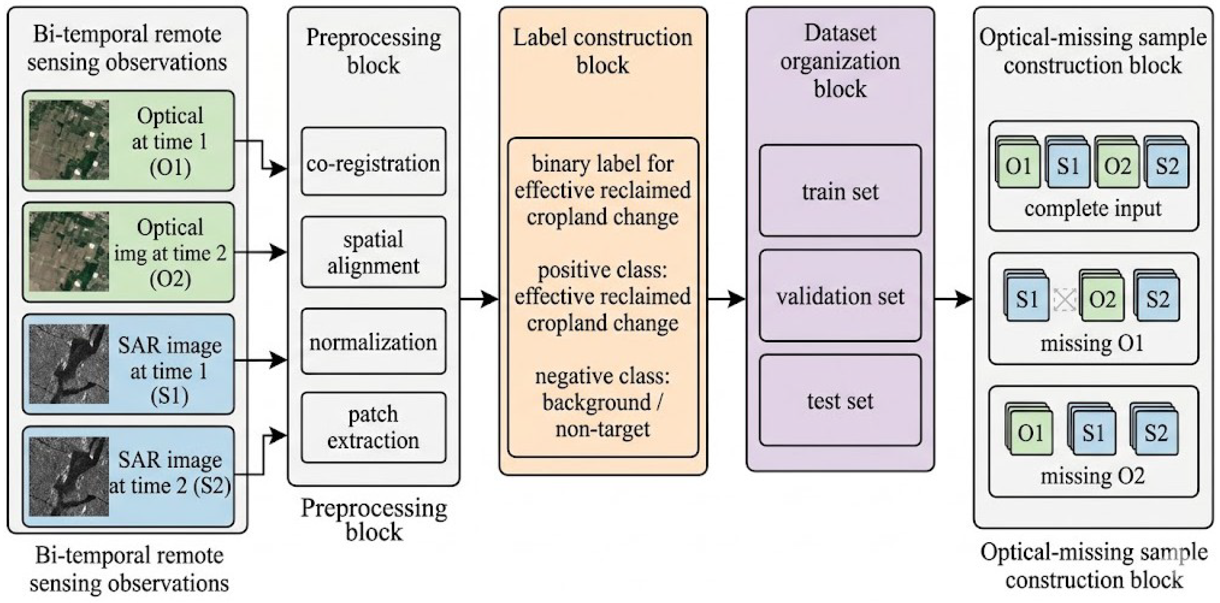
Dataset construction pipeline for effective reclaimed cropland change detection. The figure illustrates the organization of , , , and , the construction of binary reclaimed-cropland change labels, patch generation, and the training/validation/test split.
Figure 1.
Dataset construction pipeline for effective reclaimed cropland change detection. The figure illustrates the organization of , , , and , the construction of binary reclaimed-cropland change labels, patch generation, and the training/validation/test split.
Figure 2.
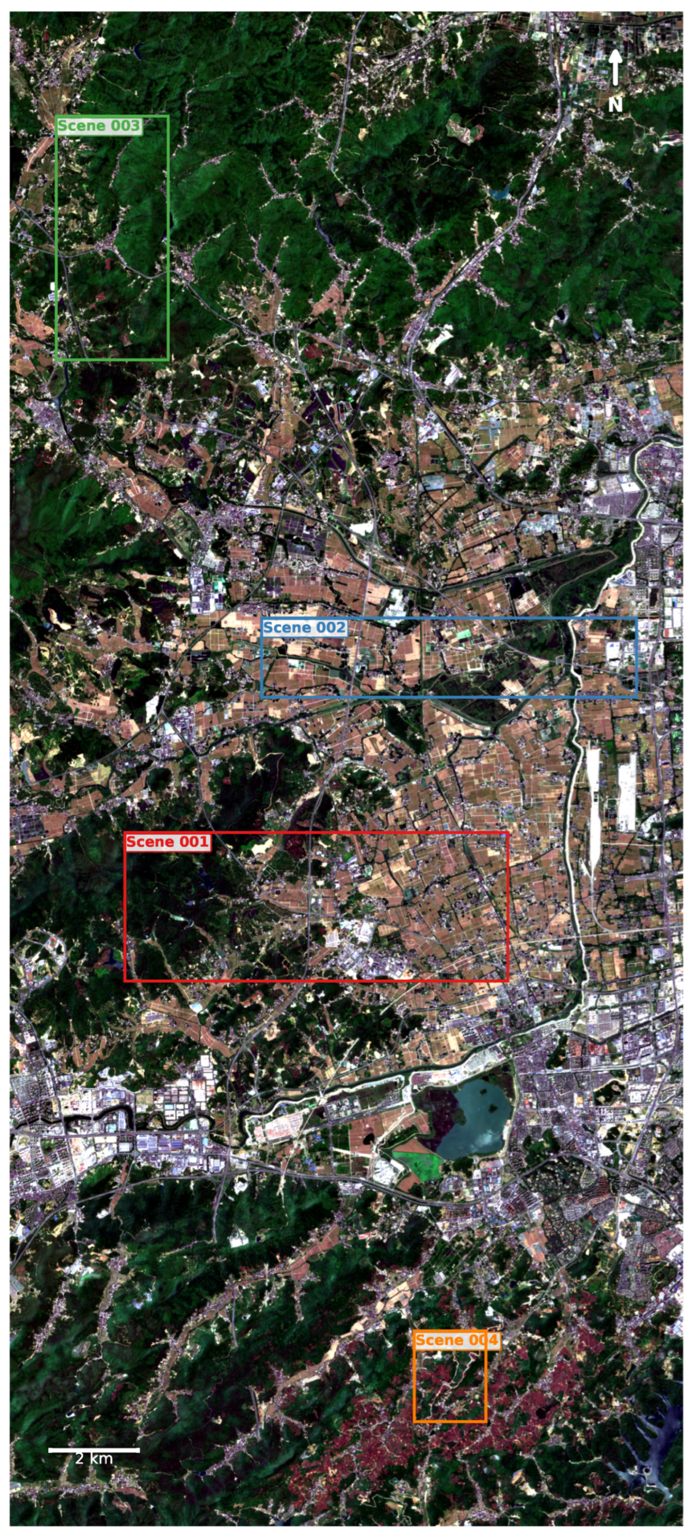
Geographic overview of the study area and the four dataset scenes. A Sentinel-2 true-color image acquired on 17 May 2024 serves as the background. The red, blue, green, and orange rectangles denote Scenes 001, 002, 003, and 004, respectively. The four labeled rectangles indicate the spatial extent of each scene, covering a total area of approximately 13 km (east–west) by 30 km (north–south) in the Hangzhou region, Zhejiang Province, China.
Figure 2.
Geographic overview of the study area and the four dataset scenes. A Sentinel-2 true-color image acquired on 17 May 2024 serves as the background. The red, blue, green, and orange rectangles denote Scenes 001, 002, 003, and 004, respectively. The four labeled rectangles indicate the spatial extent of each scene, covering a total area of approximately 13 km (east–west) by 30 km (north–south) in the Hangzhou region, Zhejiang Province, China.
Figure 3.
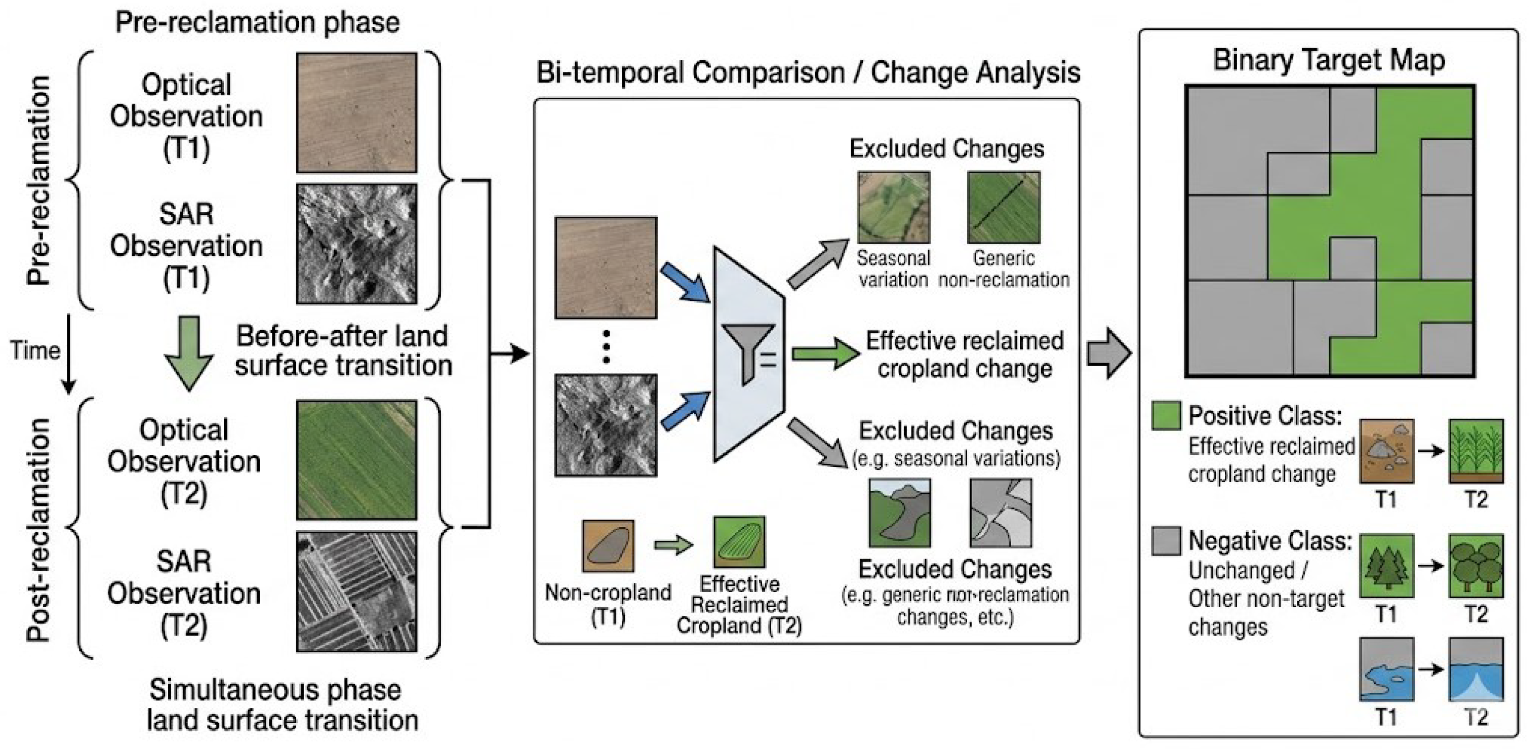
Task definition for effective reclaimed cropland detection. The figure shows how bi-temporal optical–SAR observations support the identification of effective reclaimed cropland change, and how the binary target map Y is derived from the task definition. Blue arrows indicate the optical–SAR observations entering the change-analysis module, green arrows and regions indicate effective reclaimed-cropland transitions and the positive class, and gray arrows and regions indicate excluded changes and the negative class.
Figure 3.
Task definition for effective reclaimed cropland detection. The figure shows how bi-temporal optical–SAR observations support the identification of effective reclaimed cropland change, and how the binary target map Y is derived from the task definition. Blue arrows indicate the optical–SAR observations entering the change-analysis module, green arrows and regions indicate effective reclaimed-cropland transitions and the positive class, and gray arrows and regions indicate excluded changes and the negative class.
Figure 4.
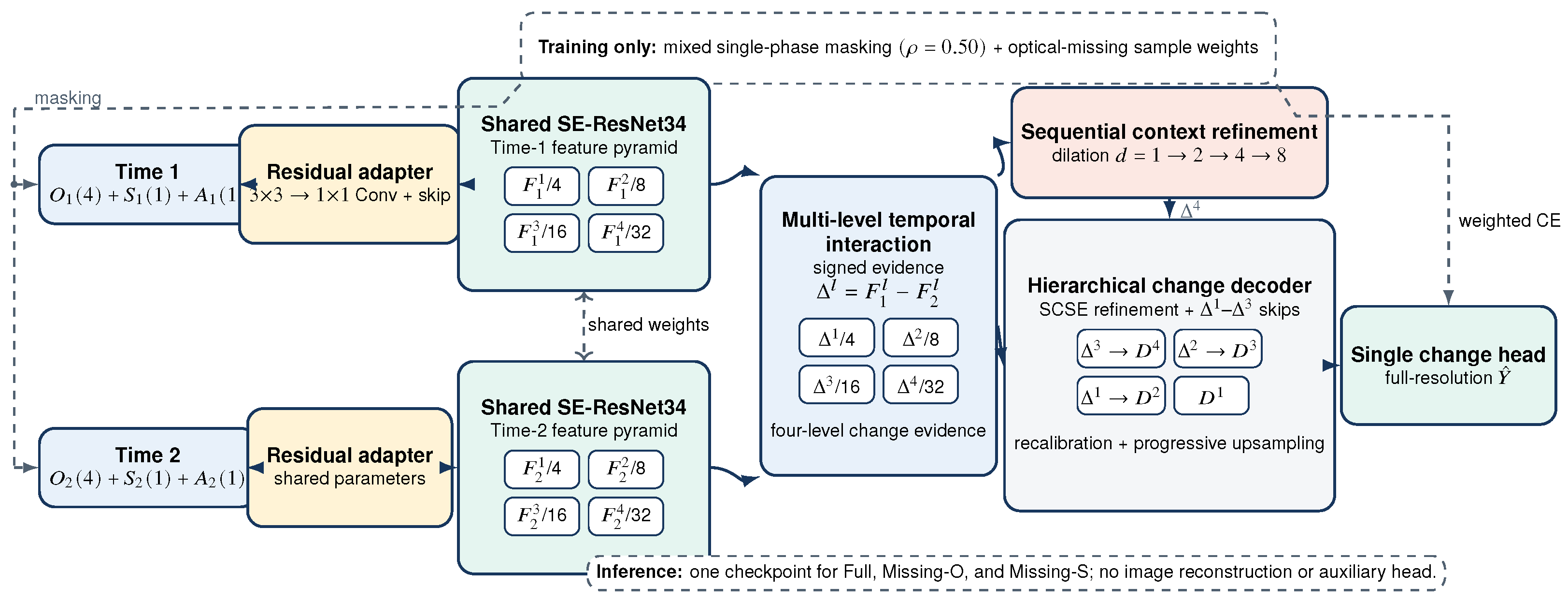
Architecture of MARC-Net. Each time point is represented by four optical channels, one SAR channel, and one availability channel. When a single phase is unavailable, condition-aware temporal proxy stabilization uses only the corresponding available observation from the other date before shared residual adaptation. The shared SE-ResNet34 encoder produces four feature levels; signed bi-temporal differences are refined by sequential dilated convolution and decoded through hierarchical SCSE blocks with multi-level difference skips. A single head predicts the full-resolution change map, while mixed missing simulation and the condition-balanced multi-state objective are used only during training.
Figure 4.
Architecture of MARC-Net. Each time point is represented by four optical channels, one SAR channel, and one availability channel. When a single phase is unavailable, condition-aware temporal proxy stabilization uses only the corresponding available observation from the other date before shared residual adaptation. The shared SE-ResNet34 encoder produces four feature levels; signed bi-temporal differences are refined by sequential dilated convolution and decoded through hierarchical SCSE blocks with multi-level difference skips. A single head predicts the full-resolution change map, while mixed missing simulation and the condition-balanced multi-state objective are used only during training.
Figure 5.
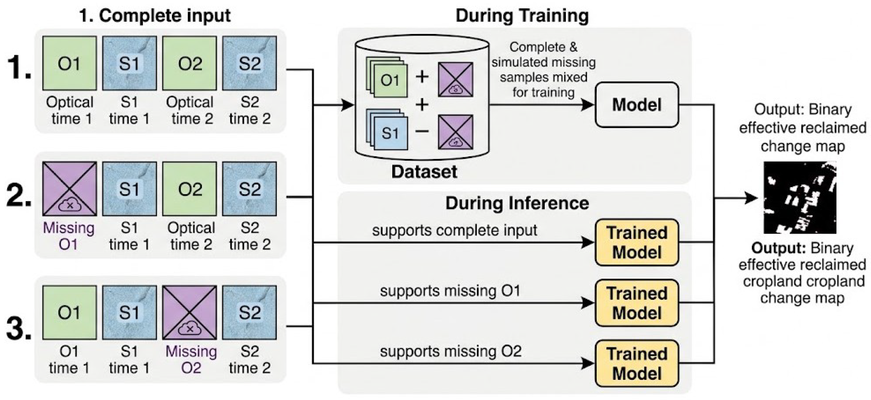
Training and inference protocol. Complete samples are mixed with single-phase optical-missing and SAR-missing samples during training. The primary evaluation removes or while retaining both SAR observations; missing-SAR inference is reported as a complementary stress test. No missing image is reconstructed.
Figure 5.
Training and inference protocol. Complete samples are mixed with single-phase optical-missing and SAR-missing samples during training. The primary evaluation removes or while retaining both SAR observations; missing-SAR inference is reported as a complementary stress test. No missing image is reconstructed.
Figure 6.
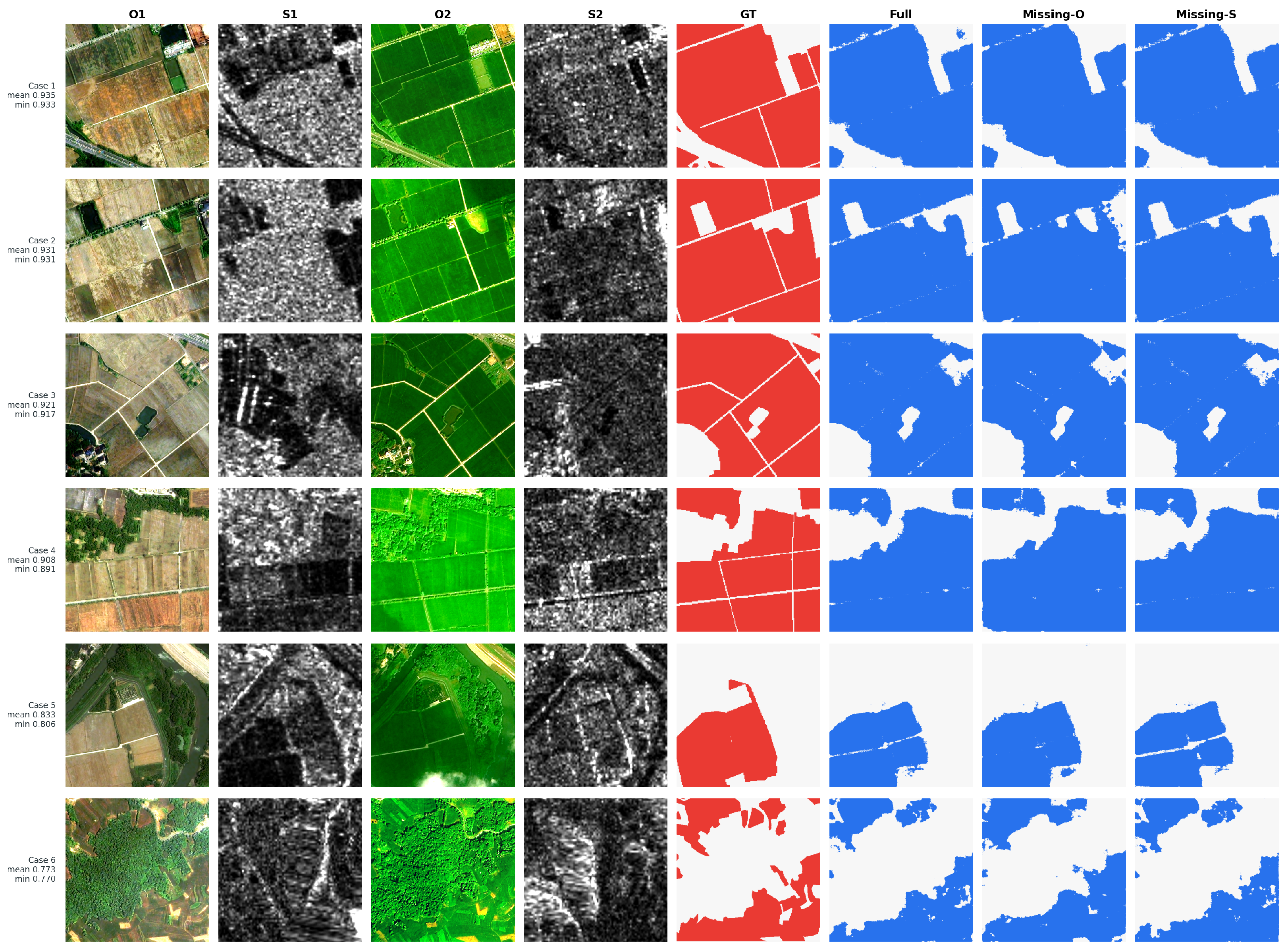
Spatially diverse robust examples from the reported MARC-Net checkpoint under Full, Missing-O, and Missing-S inference. Each row shows , , , , the ground truth, and the three predictions.
Figure 6.
Spatially diverse robust examples from the reported MARC-Net checkpoint under Full, Missing-O, and Missing-S inference. Each row shows , , , , the ground truth, and the three predictions.
Figure 7.
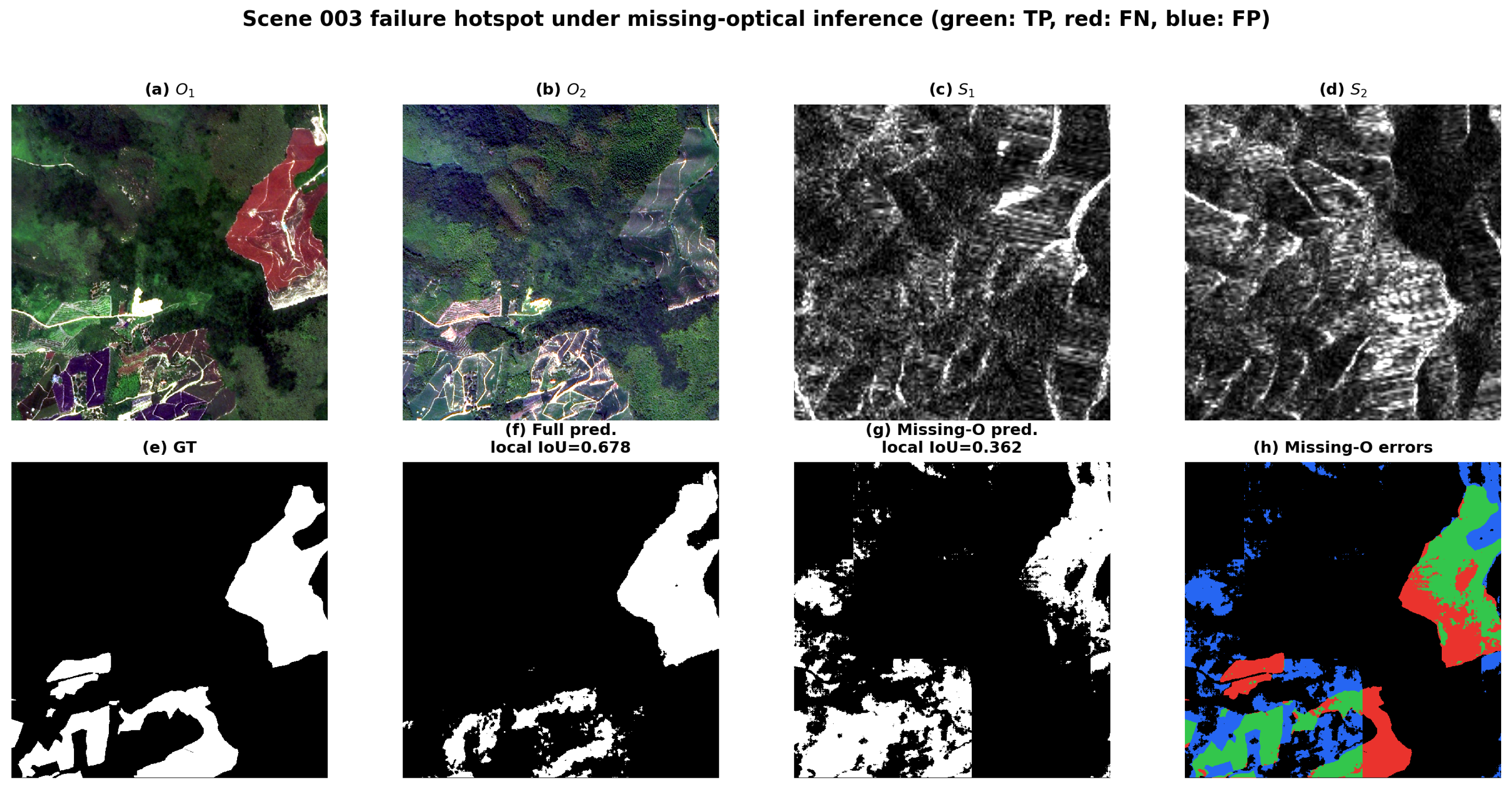
Focused challenging-case analysis for Scene 003. The panels show , , , , the ground truth, the Full prediction, the Missing-O prediction, and the Missing-O error map. Green, red, and blue denote true positives, false negatives, and false positives. Full-scene IoUs are 0.6900, 0.1410, and 0.6798 under Full, Missing-O, and Missing-S inference.
Figure 7.
Focused challenging-case analysis for Scene 003. The panels show , , , , the ground truth, the Full prediction, the Missing-O prediction, and the Missing-O error map. Green, red, and blue denote true positives, false negatives, and false positives. Full-scene IoUs are 0.6900, 0.1410, and 0.6798 under Full, Missing-O, and Missing-S inference.
Figure 8.
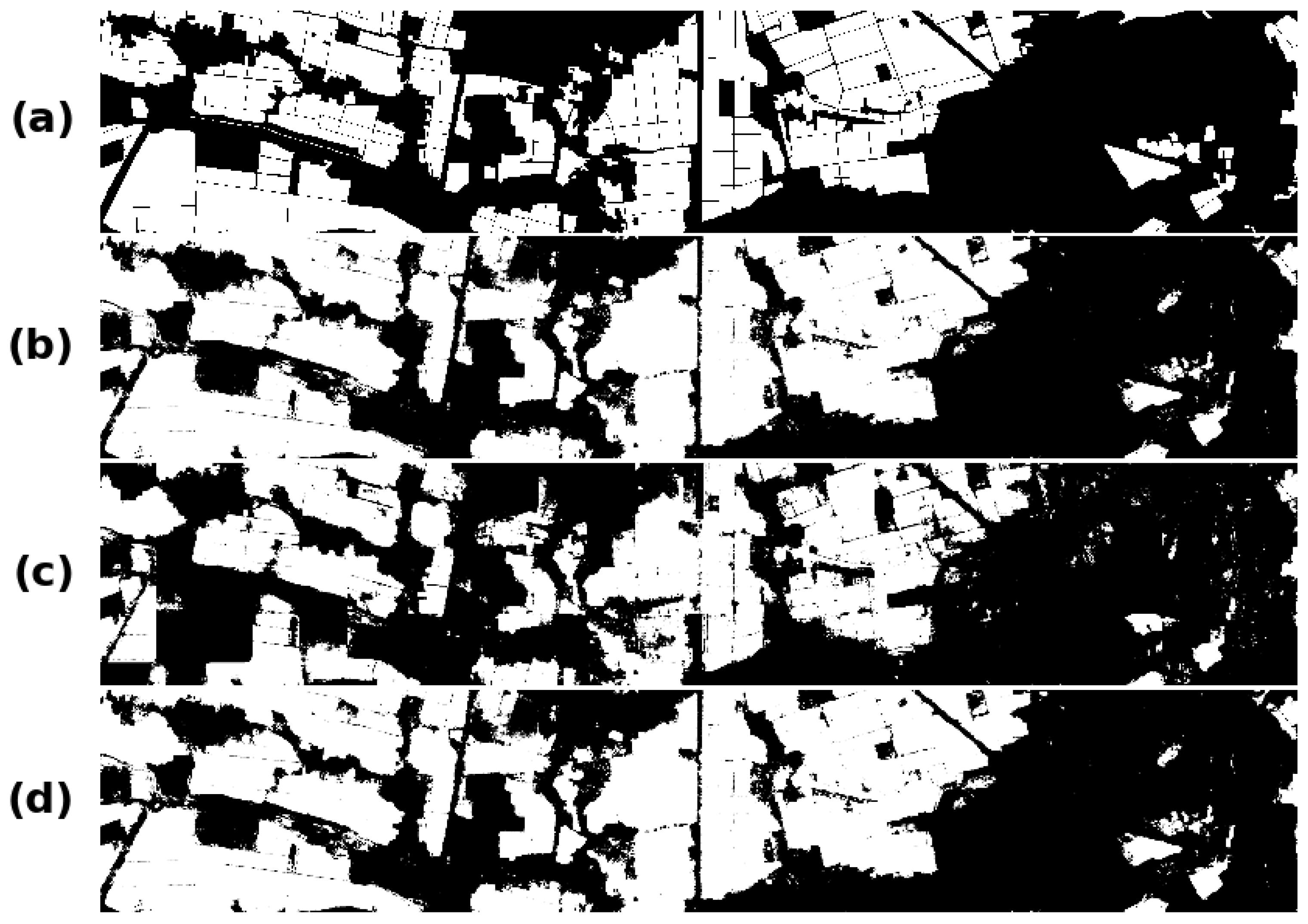
Full-scene prediction maps for Scene 002: (a) ground truth; (b) Full prediction; (c) Missing-O prediction; and (d) Missing-S prediction. White denotes detected change, and black denotes background.
Figure 8.
Full-scene prediction maps for Scene 002: (a) ground truth; (b) Full prediction; (c) Missing-O prediction; and (d) Missing-S prediction. White denotes detected change, and black denotes background.
Table 1.
Summary of the four dataset scenes. Scene IDs are used consistently throughout the experiments.
Table 1.
Summary of the four dataset scenes. Scene IDs are used consistently throughout the experiments.
| Scene | Size (Pixels) | Label Ratio (%) |
|---|
| 001 | 11,500 × 4200 | 27.0 |
| 002 | 11,300 × 2100 | 41.7 |
| 003 | | 3.9 |
| 004 | | 25.9 |
Table 2.
Dataset organization used for bi-temporal optical–SAR reclaimed cropland change detection.
Table 2.
Dataset organization used for bi-temporal optical–SAR reclaimed cropland change detection.
| Subset | Pairs | Patch Size | Modalities | Split Protocol/Description |
|---|
| Training | 1104 | | | Mixed-scene training with complete and simulated single-phase optical- or SAR-missing samples. |
| Validation | 184 | | | Complete-input model selection on the fixed mixed-scene validation split. |
| Testing | 184 | | with controlled missing settings | The same fixed test pairs are evaluated under Full, Missing-O, and Missing-S conditions. |
Table 3.
Training and implementation settings of the reported MARC-Net.
Table 3.
Training and implementation settings of the reported MARC-Net.
| Item | Setting |
|---|
| Time-point input | 4 optical + 1 SAR + 1 joint-availability channel |
| Shared encoder | SE-ResNet34, layer configuration |
| Deep context | Sequential dilated convolutions, rates |
| Decoder | Four SCSE upsampling blocks with three difference skips |
| Prediction heads | One two-class full-resolution head |
| Patch size | |
| Representation-learning phase | Adam, , 25 epochs, mixed single-phase missing simulation |
| Condition-balanced phase | FP32 AdamW, , 5 epochs |
| Condition-balanced stabilization | Weight decay ; gradient clip 2; EMA 0.995; frozen BN statistics |
| Batch sizes | Train 2/validation 8 |
| Random seed | 2022 |
| Missing target/mode | Mixed optical+SAR/single-phase either |
| // | 0.5/0.6/0.6 |
| Condition weights | Full 1.15/Missing-O 1.60/Missing-S 1.25 |
| Temporal-proxy coefficients | / |
| Checkpoint rule | Highest three-condition validation mean IoU |
| Data augmentation | Random horizontal and vertical flips |
Table 4.
Base-phase LOSO scene-level IoU and matched mixed-scene test result for MARC-Net. LOSO averages are arithmetic means over the four held-out scenes. Bold values indicate the highest IoU in each inference-condition column.
Table 4.
Base-phase LOSO scene-level IoU and matched mixed-scene test result for MARC-Net. LOSO averages are arithmetic means over the four held-out scenes. Bold values indicate the highest IoU in each inference-condition column.
| Protocol | Evaluation Set | Full IoU | Missing-O IoU | Missing-S IoU |
|---|
| LOSO | Scene 001 | 0.6970 | 0.3750 | 0.7215 |
| LOSO | Scene 002 | 0.7776 | 0.5864 | 0.7734 |
| LOSO | Scene 003 | 0.2819 | 0.1150 | 0.1812 |
| LOSO | Scene 004 | 0.6027 | 0.4904 | 0.5860 |
| LOSO | Average | 0.5898 | 0.3917 | 0.5655 |
| Mixed scene | Official test split | 0.7760 | 0.6049 | 0.7659 |
Table 5.
Base-phase training-protocol comparison of MARC-Net on the mixed-scene test set. Each inference condition reports IoU, Precision (P), and Recall (R). Bold values indicate the highest IoU in each inference-condition column.
Table 5.
Base-phase training-protocol comparison of MARC-Net on the mixed-scene test set. Each inference condition reports IoU, Precision (P), and Recall (R). Bold values indicate the highest IoU in each inference-condition column.
| Training Protocol | Full | Missing-O | Missing-S |
|---|
| | IoU | P | R | IoU | P | R | IoU | P | R |
|---|
| Train Missing Optical | 0.6704 | 0.8406 | 0.7681 | 0.5985 | 0.7849 | 0.7160 | 0.6057 | 0.7684 | 0.7410 |
| Train Missing SAR | 0.6553 | 0.8272 | 0.7592 | 0.2647 | 0.4822 | 0.3698 | 0.6600 | 0.8358 | 0.7583 |
| Train Missing Optical + SAR | 0.7760 | 0.8506 | 0.8984 | 0.6049 | 0.7814 | 0.7281 | 0.7659 | 0.8521 | 0.8833 |
Table 6.
Base-phase component-level ablation of MARC-Net under the mixed-scene protocol. Each condition reports IoU, and Mean is the unweighted average of the three IoUs. Bold values indicate the highest IoU in each column.
Table 6.
Base-phase component-level ablation of MARC-Net under the mixed-scene protocol. Each condition reports IoU, and Mean is the unweighted average of the three IoUs. Bold values indicate the highest IoU in each column.
| Variant | Controlled Change | Full | Missing-O | Missing-S | Mean |
|---|
| w/o availability signal | Availability map fixed to 1 | 0.7667 | 0.6183 | 0.7497 | 0.7116 |
| w/o input adapter | Direct six-channel encoder input | 0.7763 | 0.5106 | 0.7680 | 0.6850 |
| w/o dilated context | No deepest dilated block | 0.7719 | 0.5813 | 0.7569 | 0.7034 |
| w/o difference skips | Deepest difference only | 0.7738 | 0.6092 | 0.7391 | 0.7074 |
| MARC-Net | Complete architecture | 0.7760 | 0.6049 | 0.7659 | 0.7156 |
Table 7.
Base-phase sensitivity of MARC-Net to missing probability , simulated missing phase, and optimization loss. Each entry reports IoU. Bold values indicate the highest IoU in each column.
Table 7.
Base-phase sensitivity of MARC-Net to missing probability , simulated missing phase, and optimization loss. Each entry reports IoU. Bold values indicate the highest IoU in each column.
| Training Setting | Full | Missing-O | Missing-S | Mean |
|---|
| Reference: , either, CE | 0.7760 | 0.6049 | 0.7659 | 0.7156 |
| , either, CE | 0.7478 | 0.5509 | 0.6861 | 0.6616 |
| , either, CE | 0.7732 | 0.6325 | 0.7687 | 0.7248 |
| , fixed , CE | 0.6833 | 0.3516 | 0.6616 | 0.5655 |
| , fixed , CE | 0.7538 | 0.4795 | 0.7530 | 0.6621 |
| , either, CE + Dice | 0.7496 | 0.5716 | 0.7489 | 0.6900 |
Table 8.
Comparison of MARC-Net design variants and external supervised baselines under the mixed-scene protocol. Each inference condition reports IoU, Precision (P), and Recall (R). Bold and underlined IoU values indicate the best and second-best results, respectively, in each inference condition.
Table 8.
Comparison of MARC-Net design variants and external supervised baselines under the mixed-scene protocol. Each inference condition reports IoU, Precision (P), and Recall (R). Bold and underlined IoU values indicate the best and second-best results, respectively, in each inference condition.
| Method | Full | Missing-O | Missing-S |
|---|
| | IoU | P | R | IoU | P | R | IoU | P | R |
|---|
| Initial formulation | 0.7701 | 0.8465 | 0.8950 | 0.2988 | 0.4863 | 0.4367 | 0.7501 | 0.8392 | 0.8760 |
| FC-EF [16] | 0.7332 | 0.8801 | 0.8146 | 0.5092 | 0.8674 | 0.5522 | 0.7651 | 0.8795 | 0.8547 |
| FC-Siam-diff [16] | 0.7504 | 0.8289 | 0.8878 | 0.2869 | 0.9078 | 0.2955 | 0.7348 | 0.8052 | 0.8936 |
| DTCDSCN [17] | 0.7812 | 0.8687 | 0.8858 | 0.4578 | 0.9111 | 0.4792 | 0.7735 | 0.8595 | 0.8854 |
| ChangeFormerV6 [19] | 0.7744 | 0.8513 | 0.8956 | 0.4688 | 0.8024 | 0.5300 | 0.7772 | 0.8620 | 0.8876 |
| BIT [18] | 0.7591 | 0.9057 | 0.8243 | 0.2890 | 0.9214 | 0.2963 | 0.3792 | 0.9149 | 0.3931 |
| SwinSUNet [21] | 0.7761 | 0.8799 | 0.8681 | 0.6722 | 0.8521 | 0.7610 | 0.7659 | 0.8746 | 0.8604 |
|
ChangeMamba [22]
|
0.7434
|
0.8687
|
0.8375
|
0.3038
|
0.5071
|
0.4310
|
0.4468
|
0.7822
|
0.5103
|
| MARC-Net w/o balanced objective | 0.7760 | 0.8506 | 0.8984 | 0.6049 | 0.7814 | 0.7281 | 0.7659 | 0.8521 | 0.8833 |
| MARC-Net + consistency regularization | 0.7728 | 0.8598 | 0.8843 | 0.5397 | 0.7269 | 0.6770 | 0.7720 | 0.8622 | 0.8807 |
|
MARC-Net (proposed)
| 0.7826 |
0.8944
|
0.8622
| 0.7039 |
0.8789
|
0.7795
| 0.7780 |
0.8929
|
0.8581
|
Table 9.
Additional heterogeneous change-detection comparison under Missing-O inference on the 184-sample mixed-scene test set. Bold formatting identifies the proposed method.
Table 9.
Additional heterogeneous change-detection comparison under Missing-O inference on the 184-sample mixed-scene test set. Bold formatting identifies the proposed method.
| Method | Supervision | Available Inference Input | P | R | F1 | IoU |
|---|
| INLPG [60] | Unsupervised | – or – | 0.1944 | 0.0938 | 0.1265 | 0.0675 |
| RIEM [61] | Unsupervised | – or – | 0.2140 | 0.1204 | 0.1541 | 0.0835 |
| MARC-Net (proposed) | Supervised | Remaining optical image + | 0.8789 | 0.7795 | 0.8262 | 0.7039 |
Table 10.
Proposed MARC-Net under controlled single-phase optical degradation on the 184-sample mixed-scene test set. Affected is the mean fraction of modified pixels; the optical availability flag remains 1.
Table 10.
Proposed MARC-Net under controlled single-phase optical degradation on the 184-sample mixed-scene test set. Affected is the mean fraction of modified pixels; the optical availability flag remains 1.
| Condition | Affected (%) | P | R | F1 | IoU |
|---|
| Clean | 0.0 | 0.8944 | 0.8622 | 0.8780 | 0.7826 |
| Cloud 20% | 27.9 | 0.8933 | 0.6439 | 0.7484 | 0.5980 |
| Cloud 40% | 51.0 | 0.9000 | 0.4717 | 0.6190 | 0.4482 |
| Cloud 60% | 71.1 | 0.9095 | 0.3109 | 0.4634 | 0.3016 |
| Haze | 100.0 | 0.8874 | 0.5636 | 0.6894 | 0.5260 |
| Shadow | 40.0 | 0.9105 | 0.7591 | 0.8279 | 0.7064 |
| Radiometric | 100.0 | 0.9414 | 0.4458 | 0.6051 | 0.4338 |
Table 11.
Full-scene sliding-window IoU of the mixed-scene-trained base-phase MARC-Net. Bold formatting indicates the average across the four scenes.
Table 11.
Full-scene sliding-window IoU of the mixed-scene-trained base-phase MARC-Net. Bold formatting indicates the average across the four scenes.
| Scene | Full IoU | Missing-O IoU | Missing-S IoU |
|---|
| 001 | 0.7540 | 0.5797 | 0.7520 |
| 002 | 0.8051 | 0.6980 | 0.7948 |
| 003 | 0.6900 | 0.1410 | 0.6798 |
| 004 | 0.6323 | 0.3553 | 0.6289 |
| Average | 0.7204 | 0.4435 | 0.7139 |




 ,
,