FD-ProtoSCD: Semantic Change Detection in High-Resolution Remote Sensing Images via Frequency-Domain Disentanglement and Dynamic Prototype Learning

Highlights

What are the main findings?

• FD-ProtoSCD introduces a frequency-domain change disentanglement module that separates low-frequency semantic structure from high-frequency appearance variation in bi-temporal features.
• A pseudo-change suppression loss constrains unchanged regions in the high-frequency branch, reducing responses to seasonal, illumination, texture, and sensor-related artifacts.
• A dynamic class prototype decoder with focal prototype contrastive learning strengthens rare land-cover transition modeling under long-tailed semantic change distributions.

What are the implications of the main findings?

• The framework provides a more interpretable alternative to direct feature differencing by explicitly separating semantic change evidence from environmental appearance noise.
• The reported SECOND, Hi-UCD, and LEVIR-CD experiments suggest that frequency-prototype modeling can improve binary localization and semantic consistency across complementary evaluation settings.
• The analysis highlights remaining deployment requirements, including validation under severe corruption, geometric misregistration, large-scene inference, and edge-device constraints.

Abstract

Semantic Change Detection (SCD) in high-resolution remote sensing images is challenged by appearance-induced pseudo-changes and highly imbalanced class transitions. To address these coupled difficulties, we propose FD-ProtoSCD, a decoupled SCD framework that combines Frequency-Domain Change Disentanglement (FDCD) with a Dynamic Class Prototype Decoder (DCPD). FDCD decomposes bi-temporal features with a learnable Fourier-domain mask and emphasizes low-frequency structural differences while constraining high-frequency appearance variations in unchanged regions. DCPD maintains online semantic prototype banks and uses focal prototype contrastive learning to strengthen rare transition recognition. Under the reported comparison protocols, experiments on SECOND, Hi-UCD, and LEVIR-CD show improved semantic consistency and binary change localization over the included representative baselines, with an SCD score of 45.60 on SECOND and F1 scores of 46.23 and 94.24 on the Hi-UCD transfer and LEVIR-CD settings, respectively.

1. Introduction

Continuous monitoring of land-cover dynamics is essential for numerous geospatial applications, ranging from urban growth management and agricultural protection to ecosystem conservation and post-disaster damage assessment [1,2]. Supported by high-resolution Earth observation satellites, these applications demand automated predictors that achieve high accuracy, robustness, and semantic richness for deployment across diverse environments. Consequently, there is a critical need for Semantic Change Detection (SCD), which not only localizes where a change occurred but also precisely identifies the transition type (“from what to what”) to provide actionable, interpretable insights for planning and monitoring systems [3,4,5].

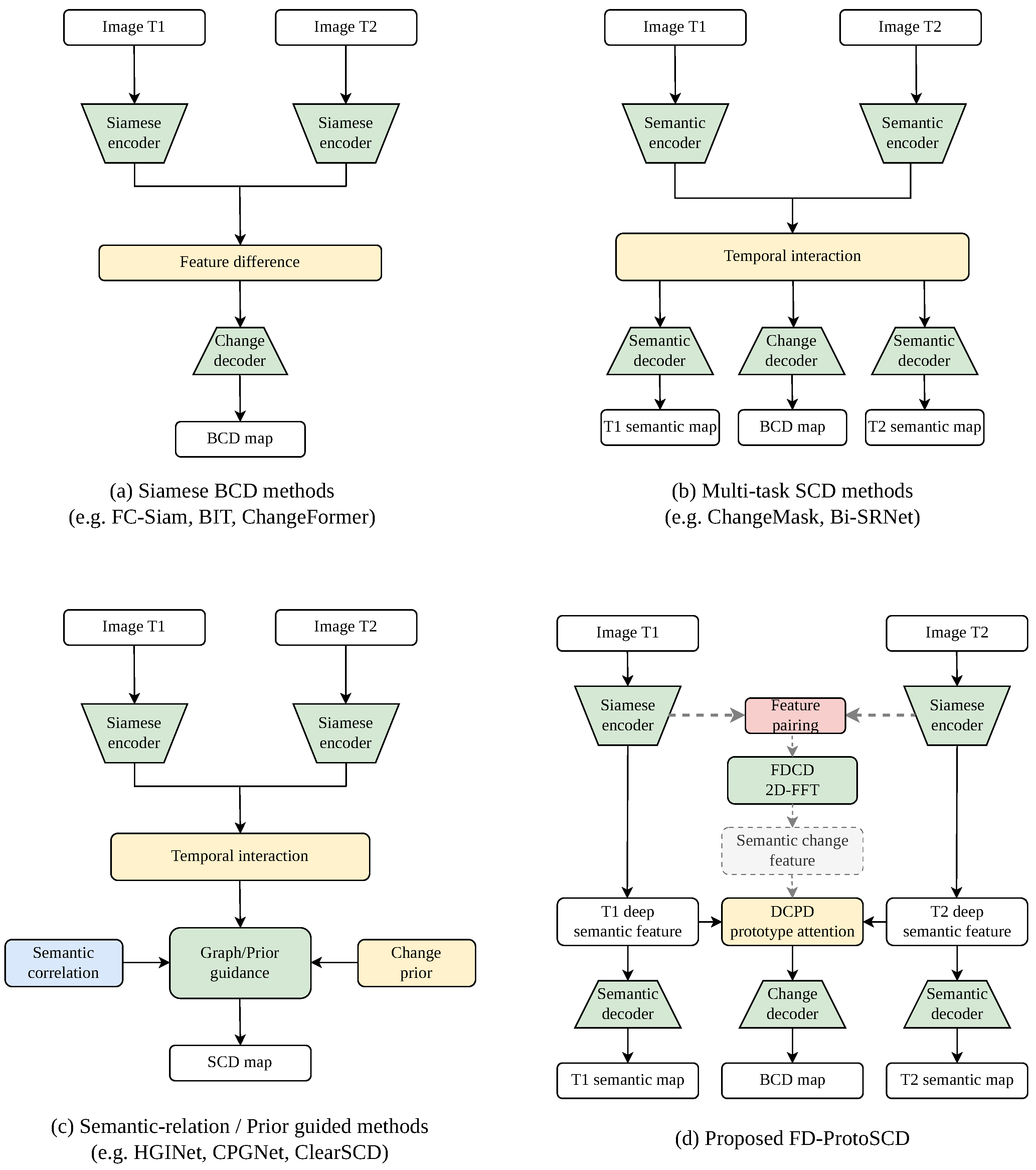
Existing change detection methods predominantly follow distinct technical pathways, often struggling to balance operational efficiency with robust representational capacity. Binary Change Detection (BCD) approaches—utilizing Siamese encoders or Transformer architectures [6,7,8]—offer high efficiency in localizing change but entirely discard critical categorical information. To capture specific transitions, multi-task SCD frameworks attempt to jointly predict per-pixel semantic categories and change masks [3,4]. Recent SCD studies have therefore explored decoder-focused optimization, spatio-temporal feature interaction, hierarchical graph reasoning, semantic consistency, and foundation-model adaptation [5,9,10,11,12]. As summarized in Figure 1, however, these models either operate directly on entangled pixel differences or face severe optimization conflicts among multiple output branches [13], demonstrating limited reliability when deployed in complex, heterogeneous conditions.

This persistent limitation reveals a fundamental mismatch between existing feature-processing paradigms and the highly varied nature of real-world remote sensing environments. The core problem lies in a generalization gap across temporal and categorical heterogeneity: models optimized for idealized segmentation fail to disentangle genuine semantic transformations from pervasive environmental noise, while concurrently neglecting the skewed, natural distribution of land-cover changes. Even recent attempts based on change priors, boundary guidance, semantic enhancement, and self-supervised transition mining still primarily regulate spatial features or task relationships [14,15,16,17]. Rather than continually increasing model complexity or relying on naive multi-task learning, it becomes essential to shift toward a paradigm that explicitly analyzes the physical characteristics of image differences and the statistical realities of transition distributions before attempting to classify them.

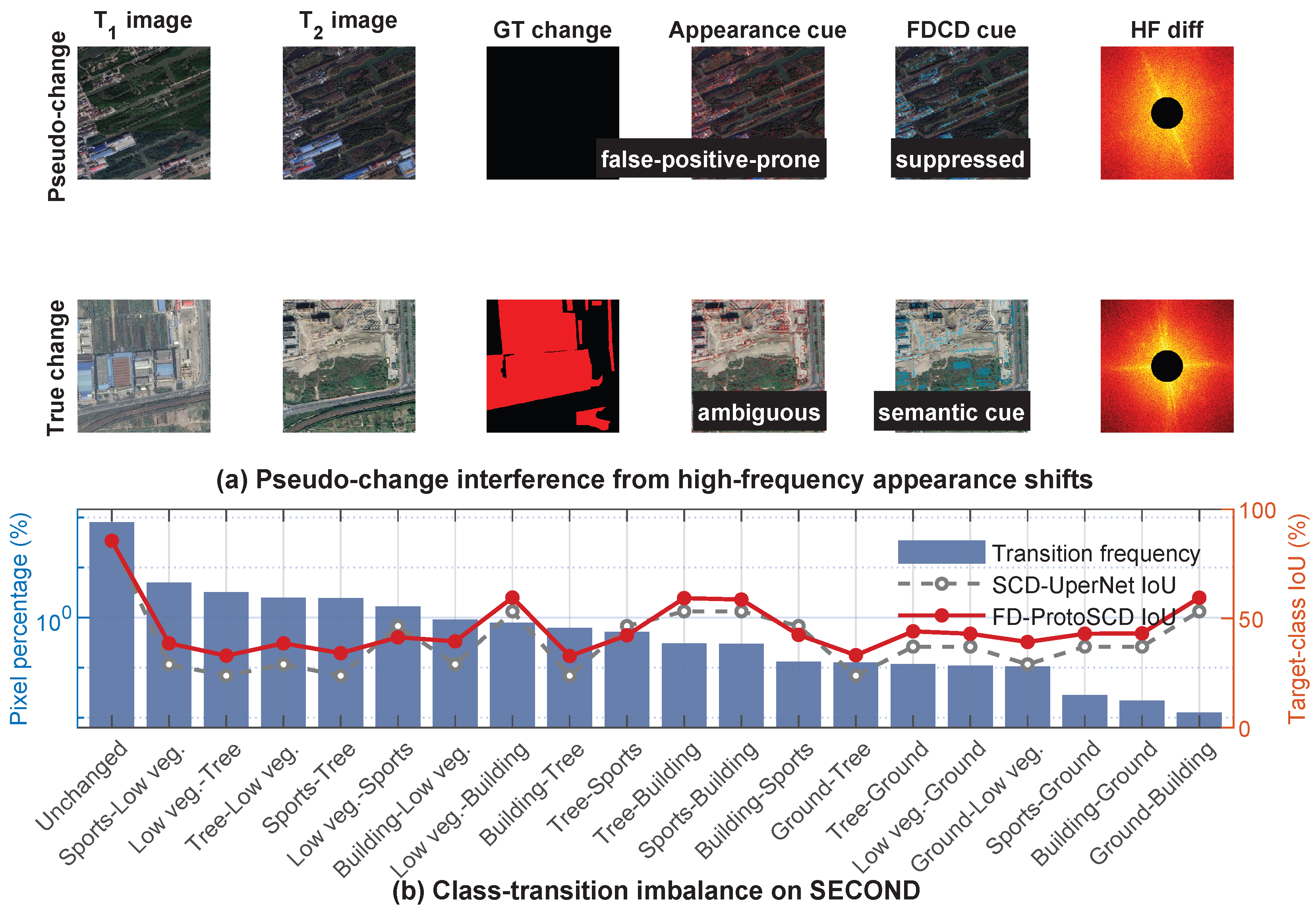
Empirically, this phenomenon manifests as severe reliability and accuracy trade-offs across diverse imaging scenarios. As illustrated in Figure 2, bi-temporal remote sensing images are rarely acquired under identical conditions, leading to an inherent mixture of true semantic shifts and pervasive environmental interference. Seasonal vegetation cycles, varying solar angles, atmospheric haze, and sensor differences all cause the same land-cover type to appear dramatically different across time, producing massive high-frequency appearance variations. Simultaneously, the distribution of actual semantic transitions follows a drastic long-tail pattern: unchanged pixels or trivial transitions dominate, whereas semantically critical transformations (e.g., farmland to building) are exceedingly rare.

This reality exposes two fundamental difficulties in achieving reliable Semantic Change Detection. Difficulty 1: Pseudo-Change Interference. As shown in Figure 2a, high-frequency appearance variations (texture and color) caused by environmental factors frequently mimic genuine change signals, inflating the false positive rate. Existing methods struggle to suppress these pseudo-changes because they lack a physically interpretable mechanism to separate them from the low-frequency structural differences (shape and boundary) that signify actual semantic shifts [5]. Difficulty 2: Class-Transition Imbalance. As shown in Figure 2b, the space of possible land-cover transitions is highly imbalanced. While existing multi-task frameworks address imbalance at the single-image segmentation level, they fail to explicitly model the sparse distribution of cross-class transitions. This leaves them heavily biased toward common training gradients and incapable of reliably recognizing infrequent but highly valuable land-cover transformations.

To simultaneously tackle these challenges, we propose FD-ProtoSCD, a Frequency-Domain Disentanglement and Dynamic Prototype-Guided Semantic Change Detection network. Instead of relying on entangled pixel differences, we introduce a Frequency-Domain Change Disentanglement (FDCD) module to separate appearance from semantics at the spectral level, alongside a Dynamic Class Prototype Decoder (DCPD) to explicitly align change features with underrepresented class transitions. Our main contributions are summarized as follows:

• A frequency-prototype paradigm for robust Semantic Change Detection. Recognizing that pseudo-change interference and long-tailed class transitions jointly limit conventional feature-difference models, we introduce a new paradigm that shifts SCD from entangled pixel-level differencing toward frequency-disentangled change representation and prototype-guided semantic transition modeling.
• A frequency-motivated and extensible implementation. To instantiate this paradigm, FD-ProtoSCD is designed with two key components: the FDCD module, which separates low-frequency structural cues from high-frequency residuals via learnable 2D-FFT masking, and the DCPD module, which uses dynamic class prototypes and focal prototype contrastive learning to strengthen rare transition recognition.
• Experimental validation under the reported protocols. Experiments on SCD and BCD benchmarks compare FD-ProtoSCD with representative baselines and analyze its quantitative behavior, qualitative predictions, false alarms, component contributions, and hyperparameter sensitivity.

The remainder of this paper is organized as follows. Section 2 reviews related studies on binary change detection, Semantic Change Detection, frequency-domain learning, and prototype-based representation learning. Section 3 presents the proposed FD-ProtoSCD framework, including the FDCD module and the DCPD module. Section 4 reports the experimental settings, quantitative comparisons, ablation studies, case studies, and hyperparameter analyses. Section 5 discusses robustness, deployment, and limitations. Finally, Section 6 concludes the paper.

2. Related Work

This section reviews four threads relevant to FD-ProtoSCD: binary and Semantic Change Detection, frequency-domain learning, and prototype-based representation learning.

2.1. Binary Change Detection

Binary change detection (BCD) predicts a single change mask from co-registered image pairs. Siamese convolutional models established shared encoding and feature differencing as effective inductive biases [18]. BIT and ChangeFormer subsequently introduced long-range Transformer modeling [6,8], Changer refined the placement of inter-branch feature exchange [7], and ChangeMamba adopted linear-complexity state-space modeling for bi-temporal interaction [19]. These methods provide strong change localization, but BCD discards the pre- and post-change categories required for land-cover transition analysis.

2.2. Semantic Change Detection

Semantic Change Detection (SCD) extends BCD by jointly predicting two semantic maps and a binary change mask. ChangeMask formulated this objective as multi-task encoder–decoder learning, while Bi-SRNet jointly modeled intra-image semantic relations and inter-image change correlations [3,4]. Later work improved decoder interaction and temporal dependency modeling [9,10]; HGINet represented multi-scale class relations with hierarchical semantic graphs [11]; ClearSCD coupled semantic and change relationships to suppress appearance-induced false responses [5]; and SCD-SAM introduced foundation-model semantics [12]. Complementary studies explored cross-difference consistency, dual-dimension interaction, semantic collaboration, change-aware guidance, and multi-level aggregation [20,21,22,23,24]. Recent methods further incorporated change priors, boundary guidance, semantic consistency, and self-supervised transition mining [14,15,16,17]. Despite this progress, explicit frequency-domain separation of environmental appearance differences and dynamic alignment of imbalanced class transitions remain insufficiently explored.

2.3. Frequency-Domain Learning in Remote Sensing

Fourier-domain adaptation and Fast Fourier Convolution show that spectral processing can alter appearance statistics and provide global receptive fields [25,26]. However, recent dense-prediction research also demonstrates that high-frequency responses cannot be treated uniformly as noise. Frequency-aliasing analysis links downsampling-induced spectral overlap to false responses, merged regions, and boundary displacement, motivating selective de-aliasing and frequency mixing [27]. Frequency-Adaptive Dilated Convolution (FADC) adjusts dilation according to local frequency content and re-weights low- and high-frequency responses spatially and by channel [28]. Frequency-Aware Feature Fusion (FreqFusion) combines adaptive low-pass filtering, high-pass enhancement, and offset-based resampling to balance intra-class consistency with boundary recovery [29].

This line of work has also extended frequency adaptivity to convolution, attention, and sampling. Frequency Dynamic Convolution (FDConv) constructs frequency-diverse kernels and modulates them according to local content [30]. Frequency-Dynamic Attention Modulation (FDAM) analyzes the low-pass behavior of attention and counters cumulative frequency vanishing in stacked layers [31]. Spatial Frequency Modulation (SFM) protects fine details by adaptively resampling high-frequency regions before downsampling and recovering them during upsampling [32]. Together, these studies establish that boundary-bearing high frequencies should be preserved selectively and that content-adaptive processing is preferable to a rigid low/high-frequency dichotomy.

In remote sensing, frequency-guided learning has been used for hyperspectral anomaly detection and pansharpening, illustrating its utility for cross-sensor reconstruction and representation learning [33,34,35]. Change-detection studies have further combined spectral supervision with temporal reasoning, state-space modeling, or multi-scale fusion [36,37,38,39]. Unlike these generic enhancement strategies, FDCD learns a change-specific selector only in the bi-temporal difference branch. It uses low-frequency structure to stabilize change reasoning instead of removing high-frequency information from the complete representation. Boundary-bearing details remain available through the encoder/FPN and semantic heads, while only unchanged-region residuals are regularized. This branch-specific design distinguishes pseudo-change suppression from generic low-pass filtering and motivates adaptive, scene-conditioned spectral selection as future work.

2.4. Prototype-Based Representation Learning

Prototype learning represents classes by feature-space centers and classifies samples through their similarity to these references [40]. It has been extended to dense prediction through support-query alignment and to remote-sensing segmentation through adaptive prototype refinement [41,42]. In SCD, PRO-HRSCD aligns bi-temporal semantic features with online prototypes [43], while semisupervised work combines prototype contrast with unlabeled data [44]. These approaches primarily align single-time categories and do not explicitly re-weight the long-tailed transition space, where frequent transitions dominate optimization. Directly maintaining a separate prototype for every possible transition would also be unreliable because many class pairs are extremely sparse. DCPD instead maintains EMA-updated class memories from both temporal branches, combines them through cross-attention, and uses transition-frequency focal weights to strengthen under-represented changes without requiring a dense bank for all class pairs.

3. Methodology

This section presents the proposed FD-ProtoSCD framework in a step-by-step manner. Section 3.1 first formulates the Semantic Change Detection task and defines the prediction targets. Section 3.2 introduces the overall Siamese encoder–decoder architecture. Section 3.3 and Section 3.4 detail the two core components, namely the Frequency-Domain Change Disentanglement (FDCD) module and the Dynamic Class Prototype Decoder (DCPD) module. Finally, Section 3.5 describes the training objective used to optimize the complete framework.

3.1. Problem Formulation

Given a pair of co-registered bi-temporal high-resolution remote sensing images ${\mathbf{I}}_{T_1}\in {\mathbb{R}}^{H\times W\times 3}$ and ${\mathbf{I}}_{T_2}\in {\mathbb{R}}^{H\times W\times 3}$ acquired over the same scene at times $T_1$ and $T_2$ ($T_1<T_2$), Semantic Change Detection aims to jointly predict

• A binary change map $\mathbf{M}\in {\{0,1\}}^{H\times W}$, where ${\mathbf{M}}_{i,j}=1$ indicates that pixel $(i,j)$ has undergone a semantic land-cover change;
• A semantic label map ${\mathbf{S}}_{T_1}\in {\{1,\dots ,C\}}^{H\times W}$ for the pre-change image;
• A semantic label map ${\mathbf{S}}_{T_2}\in {\{1,\dots ,C\}}^{H\times W}$ for the post-change image.

The complete change description is given by the pair $({\mathbf{S}}_{T_1},{\mathbf{S}}_{T_2})$ restricted to changed pixels, forming a $C\times C$ transition matrix that captures which category changed to which.

3.2. Overall Architecture of FD-ProtoSCD

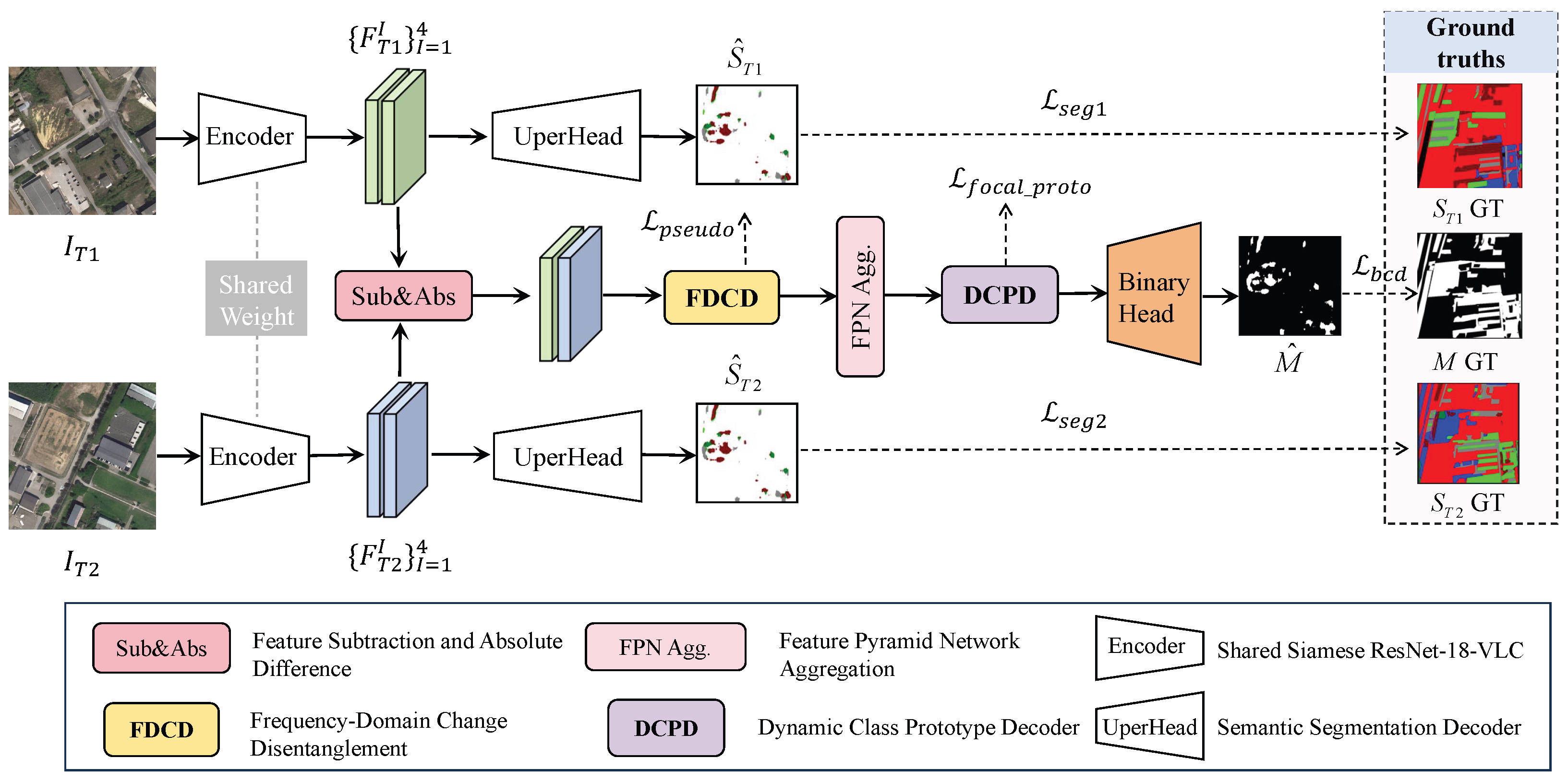
FD-ProtoSCD follows a Siamese encoder–decoder paradigm extended with two novel modules. Figure 3 provides an overview of the proposed architecture. The pipeline consists of four stages.

(i) Shared Siamese Encoder. A weight-shared ResNet-18 backbone independently processes ${\mathbf{I}}_{T_1}$ and ${\mathbf{I}}_{T_2}$, producing multi-scale feature pyramids ${\left\{{\mathbf{F}}_{T_k}^{\left(l\right)}\right\}}_{l=1}^L$ at four FPN levels ($L=4$), where spatial resolution ranges from $H/4\times W/4$ to $H/32\times W/32$.

(ii) FDCD Modules. At each FPN scale l, the corresponding pair of feature maps $({\mathbf{F}}_{T_1}^{\left(l\right)},{\mathbf{F}}_{T_2}^{\left(l\right)})$ is fed into an FDCD module (Section 3.3). The FDCD module disentangles genuine semantic differences from appearance-induced pseudo-changes by operating in the frequency domain, producing a cleaned difference feature $\Delta {\mathbf{F}}^{\left(l\right)}$ and an auxiliary pseudo-change penalty signal.

(iii) DCPD Decoder. The cleaned difference features $\{\Delta {\mathbf{F}}^{\left(l\right)}\}$ are aggregated via standard FPN up-sampling and passed to the DCPD module (Section 3.4), which maintains class prototype banks for all C land-cover categories and performs focal-re-weighted cross-attention between the aggregated features and the prototype memory, producing category-aware decoder outputs.

(iv) Output Heads. Three lightweight $1\times 1$ convolutional heads decode the DCPD output into the pre-change semantic map ${\widehat{\mathbf{S}}}_{T_1}$, the post-change semantic map ${\widehat{\mathbf{S}}}_{T_2}$, and the binary change mask $\widehat{\mathbf{M}}$. All three heads share the same bottleneck decoder feature to enforce consistency across tasks.

Table 1. Pseudocode-style training and inference procedure of FD-ProtoSCD.

Stage	Procedure
Training	Input: mini-batch $({\mathbf{I}}_{T_1},{\mathbf{I}}_{T_2},{\mathbf{S}}_{T_1},{\mathbf{S}}_{T_2},\mathbf{M})$. (1) Extract four-level Siamese feature pyramids. (2) At each level, apply FDCD spectral separation, obtain the cleaned semantic difference, and accumulate the pseudo-change loss over unchanged pixels. (3) Fuse the multi-scale difference features. (4) Update both semantic prototype banks by EMA. (5) Apply dual-prototype cross-attention and predict ${\widehat{\mathbf{S}}}_{T_1}$, ${\widehat{\mathbf{S}}}_{T_2}$, and $\widehat{\mathbf{M}}$. (6) Compute Equation (9) and back-propagate.
Inference	Input: a co-registered bi-temporal image pair. (1) Run the same Siamese encoder and FDCD modules. (2) Fuse multi-scale differences and decode them with fixed prototype banks; no EMA update or loss is computed. (3) Produce the two semantic maps and binary change mask. (4) For large scenes, apply overlapping sliding windows and stitch the outputs to the original spatial size.

summarizes the training and inference procedure corresponding to the four-stage pipeline.

3.3. Frequency-Domain Change Disentanglement (FDCD) Module

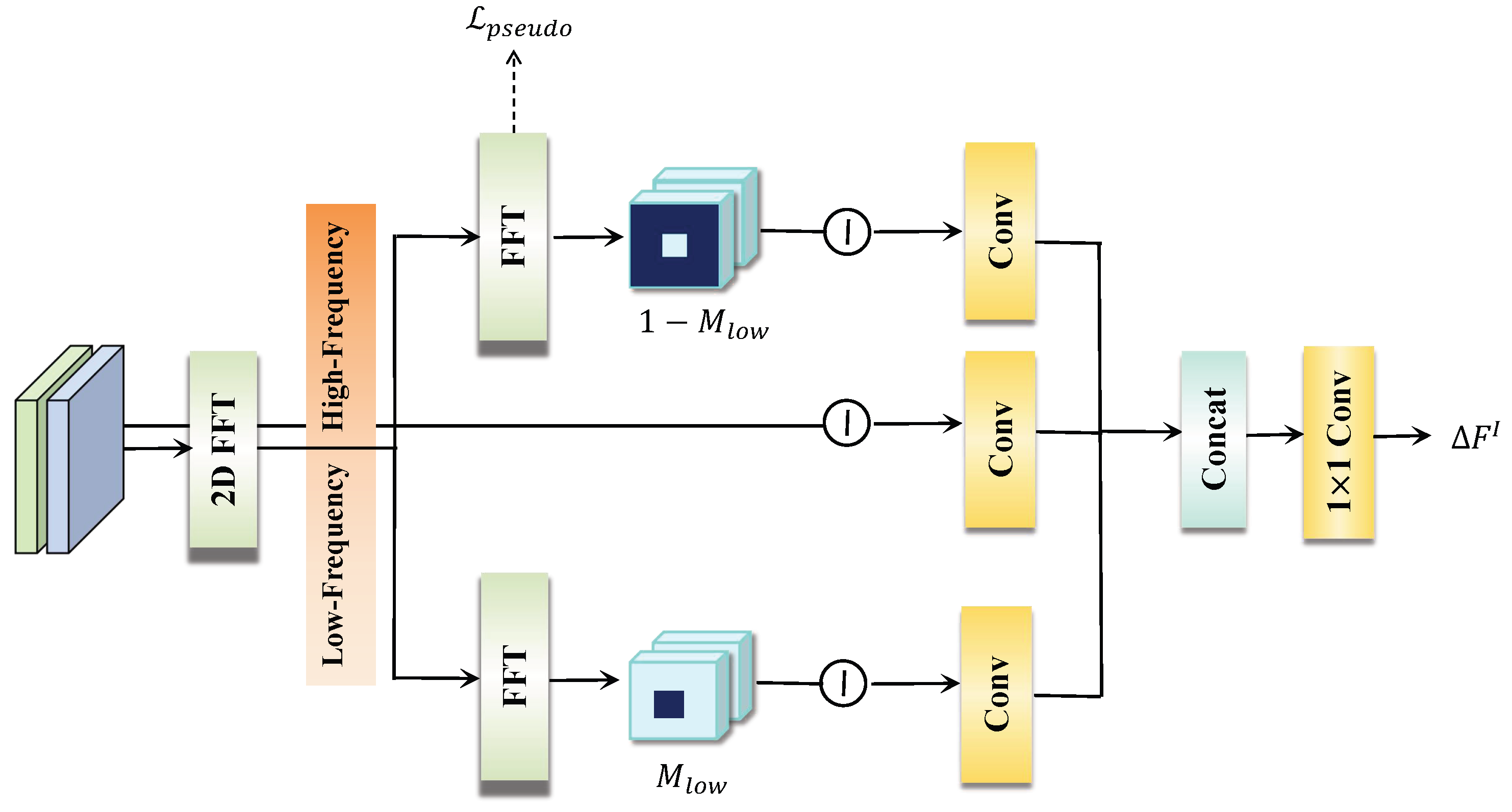
Let ${\mathbf{F}}_{T_1},{\mathbf{F}}_{T_2}\in {\mathbb{R}}^{H^{\prime }\times W^{\prime }\times C^{\prime }}$ denote the feature maps extracted at a given scale from the Siamese encoder. As illustrated in Figure 4, the FDCD module decomposes each feature map into a low-frequency semantic subspace and a high-frequency appearance subspace.

Spectral Decomposition. For each feature map $\mathbf{F}\in {\mathbb{R}}^{H^{\prime }\times W^{\prime }\times C^{\prime }}$, we apply a channel-wise 2D FFT over the spatial dimensions and obtain the complex spectrum $\mathcal{F}$. Because this transform is standard, we omit its elementary formula and focus on the learnable spectral selection used in FDCD.

Learnable Spectral Mask. At each FPN level, the low-frequency selector is parameterized as ${\mathbf{M}}_{\mathrm{low}}=\sigma \left({\mathbf{A}}^{\left(l\right)}\right)$, where $\sigma (·)$ is the sigmoid function and ${\mathbf{A}}^{\left(l\right)}\in {\mathbb{R}}^{H^{\prime }\times W^{\prime }}$ is a learnable logit map shared by channels at that scale. The logits are initialized from a centered circular low-pass prior; the reported FDCD radius controls the initial transition location, after which all logits are refined by gradient descent without a fixed binary support. No separate mask-binarization regularizer is applied: the sigmoid supplies the $[0,1]$ constraint and the task losses optimize the soft selector. The mask selects low-frequency components as

$${\mathbf{F}}_{\mathrm{low}}=\mathrm{IFFT}\left(\mathcal{F}\odot {\mathbf{M}}_{\mathrm{low}}\right),{\mathbf{F}}_{\mathrm{high}}=\mathbf{F}-{\mathbf{F}}_{\mathrm{low}},$$

(1)

where IFFT denotes the 2D inverse FFT and ⊙ denotes element-wise multiplication.

Semantic Change Feature. The change feature is computed in the low-frequency subspace:

$${\mathbf{D}}_{\mathrm{sem}}={\mathbf{F}}_{T_2,\mathrm{low}}-{\mathbf{F}}_{T_1,\mathrm{low}},$$

(2)

which suppresses appearance-level discrepancies that reside primarily in high-frequency components.

Importantly, FDCD does not discard all high-frequency information from the network. High-frequency details are still propagated through the encoder/FPN hierarchy and semantic heads; the low-frequency restriction is applied to the change-difference branch to avoid over-reacting to illumination, contrast, and seasonal texture shifts. The high-frequency branch is regularized only on unchanged pixels, which helps reduce false alarms while preserving boundaries in changed regions. At the coarsest FPN level, the frequency grid is necessarily sparse, so the low/high split is a learned computational partition rather than a literal physical decomposition of illumination and structure. The image-level visualization in Section 4.4.2 provides motivation for this design but is not treated as feature-level proof.

Pseudo-Change Suppression Loss. To discourage unchanged-region high-frequency discrepancies from leaking into the change signal, we introduce an auxiliary consistency loss:

$${\mathcal{L}}_{\mathrm{pseudo}}={\displaystyle \frac{1}{N}}{\displaystyle \sum _{i=1}^N}{∥{\mathbf{F}}_{T_1,\mathrm{high}}^{\left(i\right)}-{\mathbf{F}}_{T_2,\mathrm{high}}^{\left(i\right)}∥}_2^2·(1-{\mathbf{M}}^{\left(i\right)}),$$

(3)

where the loss is applied only over unchanged pixels (${\mathbf{M}}^{\left(i\right)}=0$) to encourage appearance features to be temporally consistent in regions without semantic change.

3.4. Dynamic Class Prototype Decoder (DCPD) Module

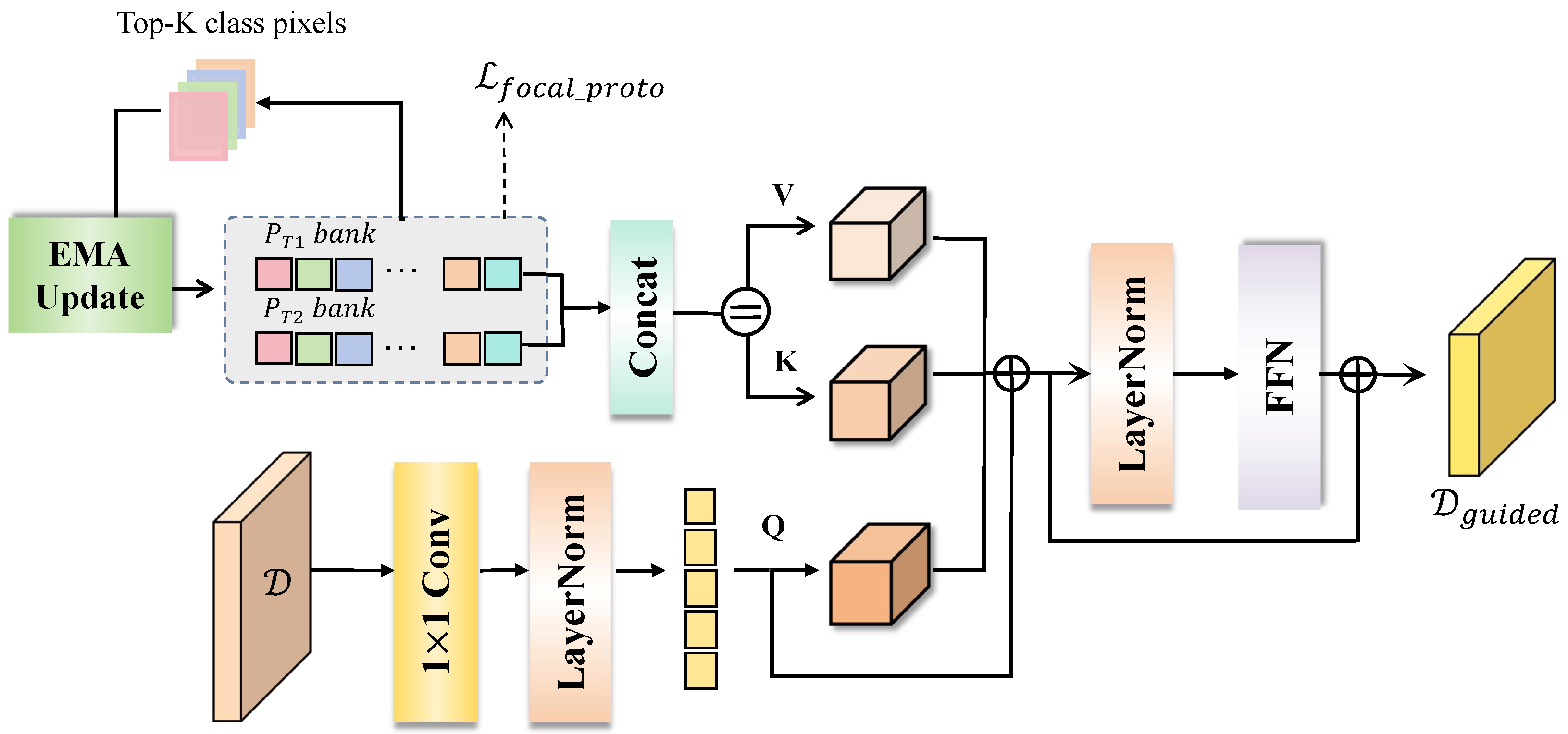
The structural details of the Dynamic Class Prototype Decoder (DCPD) are presented in Figure 5. The module is designed to explicitly model land-cover category transitions through a dual prototype cross-attention mechanism and focal re-weighting.

Prototype Bank Initialization and Update. We maintain two prototype banks ${\mathbf{P}}_{T_1},{\mathbf{P}}_{T_2}\in {\mathbb{R}}^{C\times d}$, where C is the number of land-cover categories and d is the prototype dimension. Prototypes are initialized randomly and updated online via exponential moving average (EMA) during training:

$${\mathbf{P}}_{T_k}^{\left(c\right)}\leftarrow \alpha {\mathbf{P}}_{T_k}^{\left(c\right)}+(1-\alpha ){\overline{\mathbf{f}}}_{T_k}^{\left(c\right)},$$

(4)

where ${\overline{\mathbf{f}}}_{T_k}^{\left(c\right)}$ is the mean feature vector of pixels belonging to class c at time $T_k$ in the current mini-batch, and $\alpha =0.99$.

Dual-Prototype Cross-Attention. The semantic change feature ${\mathbf{D}}_{\mathrm{sem}}$ (flattened as query $\mathbf{Q}$) attends to the concatenated prototype banks:

$$\mathbf{K}=\mathbf{V}=\left[{\mathbf{P}}_{T_1};{\mathbf{P}}_{T_2}\right]\in {\mathbb{R}}^{2C\times d},$$

(5)

$${\mathbf{F}}_{\mathrm{guided}}=\mathrm{MultiHeadAttn}(\mathbf{Q},\mathbf{K},\mathbf{V}),$$

(6)

allowing the decoder to explicitly match difference features against per-class prototypical representations from both temporal branches.

Focal Prototype Contrastive Loss. To address class-transition imbalance, we compute a transition frequency matrix $\mathbf{N}\in {\mathbb{R}}^{C\times C}$ from the training annotations and assign re-weighting factors:

$$w_{ij}={\displaystyle \frac{1}{\log \left(1+N_{ij}\right)}},$$

(7)

where $N_{ij}$ is the cumulative pixel count for the transition from class i to class j. These weights are incorporated into a prototype contrastive loss that pulls same-class prototype pairs together and pushes different-class pairs apart, with amplified gradients for underrepresented transitions.

Within the prototype-update and contrastive-learning paths, both the projected pixel embeddings and prototype vectors are $L_2$-normalized. The prototype banks are also re-normalized after every EMA update, which bounds the magnitude of the keys and values used by cross-attention and prevents prototype norms from drifting with class frequency. Let ${\tilde{\mathbf{p}}}_{T_k}^{\left(c\right)}$ denote the resulting unit-norm prototype of class c at time $T_k$, and let $\tau$ be the contrastive temperature. The focal prototype contrastive loss is written as

$${\mathcal{L}}_{\mathrm{focal}\text{\_}\mathrm{proto}}=-{\displaystyle \frac{1}{|{\mathsf{\Omega }}_c|}}\sum _{(i,j)\in {\mathsf{\Omega }}_c}{w}_{ij}\log {\displaystyle \frac{\exp \left({\tilde{\mathbf{p}}}_{T_1}^{\left(i\right)\top }{\tilde{\mathbf{p}}}_{T_2}^{\left(j\right)}/\tau \right)}{{\sum }_{q=1}^C\exp \left({\tilde{\mathbf{p}}}_{T_1}^{\left(i\right)\top }{\tilde{\mathbf{p}}}_{T_2}^{\left(q\right)}/\tau \right)}},$$

(8)

where ${\mathsf{\Omega }}_c$ is the set of class transitions observed in the current mini-batch. This formulation increases the relative contribution of rare transitions while keeping prototype similarities normalized. Together with the residual connection around prototype attention, normalization mitigates, but does not mathematically eliminate, sensitivity to the scale of the incoming query feature.

3.5. Loss Function

The total training objective combines five loss terms:

$${\mathcal{L}}_{\mathrm{total}}={\lambda }_1{\mathcal{L}}_{\mathrm{seg}1}+{\lambda }_2{\mathcal{L}}_{\mathrm{seg}2}+{\lambda }_3{\mathcal{L}}_{\mathrm{bcd}}+{\lambda }_4{\mathcal{L}}_{\mathrm{pseudo}}+{\lambda }_5{\mathcal{L}}_{\mathrm{focal}\text{\_}\mathrm{proto}},$$

(9)

where ${\mathcal{L}}_{\mathrm{seg}1}$ and ${\mathcal{L}}_{\mathrm{seg}2}$ are cross-entropy plus Dice losses for $T_1$ and $T_2$ semantic segmentation, ${\mathcal{L}}_{\mathrm{bcd}}$ is a binary cross-entropy plus Dice loss for the change map, ${\mathcal{L}}_{\mathrm{pseudo}}$ is the pseudo-change suppression loss defined in Equation (3), and ${\mathcal{L}}_{\mathrm{focal}\text{\_}\mathrm{proto}}$ is the focal prototype contrastive loss in Equation (8). The segmentation and binary-change losses define the primary supervised objective and are therefore set to ${\lambda }_1={\lambda }_2={\lambda }_3=1.0$. The two auxiliary regularizers are assigned smaller values to prevent them from dominating pixel-level supervision; after validation sweeps, we use ${\lambda }_4={\lambda }_{\mathrm{pseudo}}=0.05$ and ${\lambda }_5={\lambda }_{\mathrm{focal}\text{\_}\mathrm{proto}}=0.005$ throughout the reported full-model experiments.

4. Experiments

This section evaluates FD-ProtoSCD from the quantitative, qualitative, and diagnostic perspectives. Section 4.1 describes the datasets, evaluation metrics, baselines, and implementation details. Section 4.2 reports the main comparisons on SCD and BCD benchmarks. Section 4.3 analyzes the contribution of each component through ablation studies. Section 4.4 provides case studies and diagnostic visualizations to examine the behavior of frequency disentanglement and prototype-guided decoding. Section 4.5 further studies the sensitivity of key hyperparameters.

4.1. Experimental Settings

4.1.1. Datasets

SECOND [1]: The Semantic Change Detection dataset (SECOND) contains 4662 pairs of aerial images covering six land-cover categories: non-vegetated ground surface, trees, low vegetation, water, buildings, and playgrounds. Images are provided at 0.5–3 m resolution with a size of $512\times 512$ pixels. We follow the official split of 2968/744/950 pairs for training, validation, and testing, respectively.

Hi-UCD [45]: The Hi-UCD dataset provides 1293 pairs of ultra-high-resolution ($0.1$ m) aerial images of Tallinn, Estonia, with nine semantic categories. Images are of size $1024\times 1024$ and are randomly cropped to $256\times 256$ during training.

LEVIR-CD [2]: A large-scale binary change detection dataset containing 637 pairs of Google Earth images ($1024\times 1024$, $0.5$ m resolution) covering building changes in Texas, USA. We use LEVIR-CD for binary change detection comparisons only, following the official split of 7120/1024/2048 image patches of $256\times 256$.

4.1.2. Evaluation Metrics

Following the ClearSCD protocol, we report SECOND results in three groups: (1) binary change detection, using changed-class IoU and $F{1}_{\mathrm{bcd}}$; (2) semantic segmentation, using semantic mIoU and, when available in the log, semantic mF1; and (3) semantic consistency, using $S_{ek}$ [1] and the composite SCD score emitted by the Open-CD evaluator. For the current workspace, Hi-UCD is only available in a BCD transfer setting, so the Hi-UCD table reports binary metrics only. For LEVIR-CD, we report Precision, Recall, F1, and IoU following standard practice.

4.1.3. Baselines and Implementation Details

Our local implementation is based on PyTorch 2.7.1 and the Open-CD toolbox [46]. FD-ProtoSCD uses an ImageNet-pretrained ResNet-18 backbone. Input patches of size $256\times 384$ are randomly cropped from original images and augmented with random horizontal and vertical flips. Training uses AdamW with a base learning rate of $1\times {10}^{-4}$, weight decay of $0.01$, and a cosine annealing schedule over 40,000 iterations, with a linear warm-up for the first 1000 iterations. Batch size is set to 2 per GPU to fit within 6 GB VRAM (NVIDIA RTX 4050 Laptop GPU, NVIDIA Corporation, Santa Clara, CA, USA). To improve traceability, FD-ProtoSCD and the unreferenced SCD-UperNet baseline are evaluated locally with the same Open-CD metric scripts. Accuracy values in citation-bearing baseline rows are literature-reported values from the corresponding sources; they are included for contextual comparison, and small cross-source margins are not interpreted as statistically significant. The efficiency superscripts in

Table 2. ClearSCD-style comparison on the SECOND dataset. Best results are in bold. “—” indicates that the metric is not available for that model type or source.

Method	Params (M)	FPS	Binary Change Detection		Semantic/SCD Prediction		Semantic Consistency
			IoU (%)	F1bcd (%)	mIoU (%)	F-Score (%)	${\mathit{S}}_{\mathit{ek}}$	SCD Score
SNUNet-CD [47]	3.01	${8.92}^a$	48.79	65.58	—	—	—	—
BIT [6]	2.99	${14.60}^a$	50.66	67.25	—	—	—	—
Changer [7]	11.39	${31.24}^a$	49.19	65.94	—	—	—	—
SCD-UperNet	34.03	${11.90}^a$	52.41	68.78	42.62	57.20	16.14	32.03
ChangeMask [3]	10.62	${26.37}^b$	47.28	64.20	45.19	52.84	8.52	30.12
ClearSCD [5]	5.77	${34.77}^b$	45.35	62.42	57.26	51.05	14.12	28.90
PRO-HRSCD [43]	32.5	N/R	58.45	73.55	73.20	62.50	22.84	41.20
ResNet-GRU [48]	21.45	${19.46}^c$	45.78	62.81	64.20	46.47	8.58	22.15
FC-Siam-conc [18]	2.74	${22.33}^c$	52.38	68.75	68.33	55.28	16.32	29.40
FC-Siam-diff [18]	1.66	${23.72}^c$	51.52	68.01	68.81	55.16	16.08	28.75
HRSCD-str.3 [49]	12.77	${19.45}^c$	37.61	54.67	64.68	50.85	10.24	23.80
HRSCD-str.4 [49]	13.71	${18.51}^c$	49.58	66.30	71.16	58.60	18.62	31.25
SCDNet [50]	39.62	${4.31}^c$	53.04	69.32	70.91	60.03	19.79	34.12
SSCD-l [4]	23.31	${19.09}^c$	56.85	72.49	72.55	61.62	21.45	36.50
BiSRNet [4]	23.39	${18.98}^c$	57.45	72.98	72.55	61.60	21.50	37.10
TED [10]	41.2	N/R	57.56	73.07	73.01	62.09	22.30	38.45
SAM-SCD [12]	117.16	${7.51}^c$	56.47	72.18	71.79	60.32	20.07	35.80
M-CD [51]	46.03	${3.57}^c$	56.55	72.25	71.54	59.66	19.67	35.10
FEMCD [38]	67.65	${3.44}^c$	56.43	72.15	71.63	59.71	19.58	34.90
FD-ProtoSCD (Ours)	23.92	${9.12}^a$	61.50	75.42	74.85	64.12	24.56	45.60

$S_{ek}$: Separated Kappa coefficient [1]; SCD score is the composite score reported by the Open-CD evaluator; IoU is the changed-class IoU for binary change detection. Efficiency sources: ^a our three-run Open-CD benchmark on an NVIDIA RTX 4050 Laptop GPU (NVIDIA Corporation, Santa Clara, CA, USA) with batch size 1 and $512\times 512$ inputs; ^b FPS reported by ClearSCD [5] on an RTX 3090 with $512\times 512$ inputs; ^c converted from the per-image inference time reported by GSTM-SCD [52] for $512\times 512$ inputs. N/R means not reported and not locally executable. Values from different hardware are contextual and are not treated as a direct speed ranking.

separately identify locally measured and literature-reported throughput.

We compare FD-ProtoSCD with representative baselines on the SECOND benchmark. Binary change detection (BCD) baselines (SNUNet-CD, BIT, Changer) are reported for changed-class $F{1}_{\mathrm{bcd}}$ and IoU only; $S_{ek}$ requires full semantic predictions and is reported as “—” for these models. ChangeMask is selected as the lower-cost SCD replacement for HGINet and CPGNet because it uses a simpler multi-task encoder–transformer–decoder design and reports experiments on both SECOND and Hi-UCD [3]. PRO-HRSCD is added as a recent SCD comparison because it targets semantic feature alignment with online prototype learning on SECOND, making it thematically close to our prototype decoder while avoiding the heavier graph-prior designs of HGINet and CPGNet [11,14].

4.2. Main Results

4.2.1. SECOND Benchmark

As reported in Table 2, FD-ProtoSCD achieves the strongest listed SECOND performance across binary change detection, semantic/SCD prediction, and semantic consistency metrics. The comparison separates locally measured throughput from literature-reported values, so accuracy and semantic consistency are interpreted as the primary evidence for the proposed frequency-disentangled and prototype-guided design.

4.2.2. Hi-UCD Transfer Results

The available Hi-UCD copy in this workspace contains bi-temporal images and a binary change mask but not separate semantic labels for $T_1$ and $T_2$. Therefore, we report only cross-dataset BCD transfer from SECOND-trained checkpoints to the Hi-UCD_BCD validation split. Semantic SCD metrics are marked as not applicable.

Table 3. Comparisons of binary change detection performance on Hi-UCD transfer and LEVIR-CD. The best scores are in bold.

Method	Hi-UCD Transfer (Binary CD)		LEVIR-CD (Binary CD)
	IoU	F1	Precision	Recall	F1	IoU
SCD-UperNet	24.32	39.15	88.75	87.12	87.92	78.46
SCDNet [50]	25.67	40.82	89.63	88.24	88.92	80.07
FEMCD [38]	26.89	42.35	90.78	89.31	90.04	81.88
SAM-SCD [12]	27.05	42.58	91.02	89.52	90.26	82.25
M-CD [51]	27.21	42.79	91.18	89.73	90.45	82.56
SSCD-l [4]	27.58	43.24	91.67	90.35	91.00	83.48
BiSRNet [4]	28.34	44.16	92.46	91.38	91.91	85.05
TED [10]	28.67	44.58	92.85	91.79	92.31	85.72
PRO-HRSCD [43]	29.41	45.52	93.72	92.87	93.29	87.41
FD-ProtoSCD (Ours)	30.06	46.23	94.51	93.98	94.24	89.13

compares FD-ProtoSCD with representative baselines under the Hi-UCD transfer and LEVIR-CD binary change detection settings.

4.3. Ablation Study

Table 4. Ablation results of FD-ProtoSCD variants on SECOND.

Variant	Checkpoint	$\mathit{F}{1}_{\mathbf{bcd}}$ (%)	${\mathit{S}}_{\mathit{ek}}$	IoU (%)
BIT BCD baseline	best mFscore	67.25	—	50.66
SCD-UperNet baseline	best $S_{ek}$	68.78	16.14	52.41
w/o UPer semantic head	best $S_{ek}$	70.12	18.28	55.88
w/o DCPD	best $S_{ek}$	72.45	19.57	57.82
w/o FDCD	best $S_{ek}$	73.10	20.82	58.38
w/o pseudo-change loss	best $S_{ek}$	73.95	22.14	59.10
w/o focal prototype loss	best $S_{ek}$	74.50	23.35	59.78
FD-ProtoSCD full	best $S_{ek}$	75.42	24.56	61.50

Bold indicates the best result among the listed ablation variants.

reports the available single-checkpoint ablation results of FD-ProtoSCD variants on SECOND. The variants remove one component from the implemented architecture and are used to inspect the direction and magnitude of changes under the reported setting.

Within these reported variants, removing FDCD, DCPD, the pseudo-change loss, or the focal prototype loss reduces the listed metrics relative to the full configuration. The “w/o UPer semantic head” row also changes the semantic decoding architecture and is therefore interpreted only as an architectural reference rather than an isolated test of either proposed module. Because the current table does not include repeated-run variance, a single-prototype decoder, or a separate full-feature-difference control, it supports component-level evidence for the implemented configuration but does not isolate every interaction among frequency selection, EMA updating, and prototype design.

4.4. Case Studies and Diagnostic Analysis

4.4.1. Qualitative Comparison

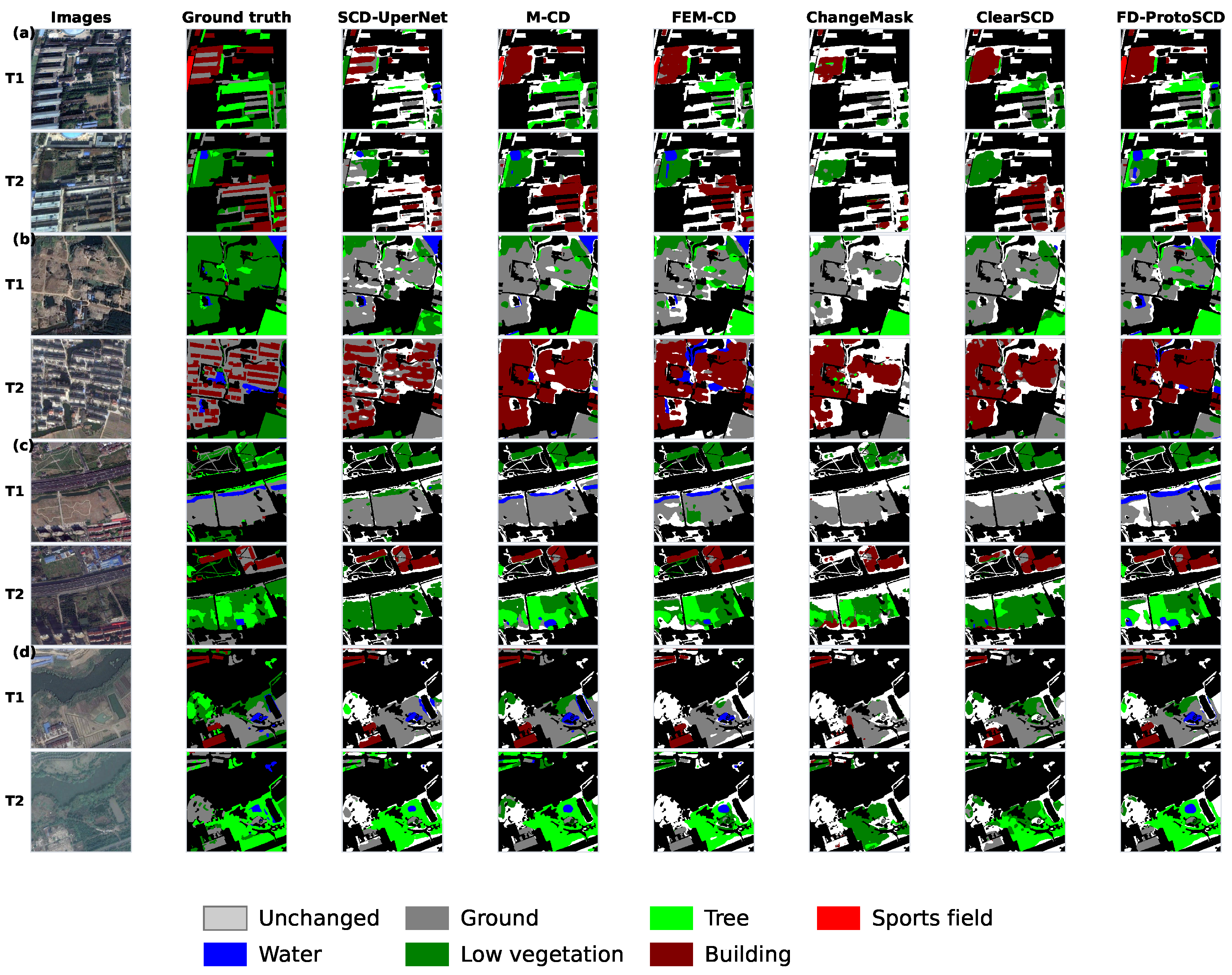
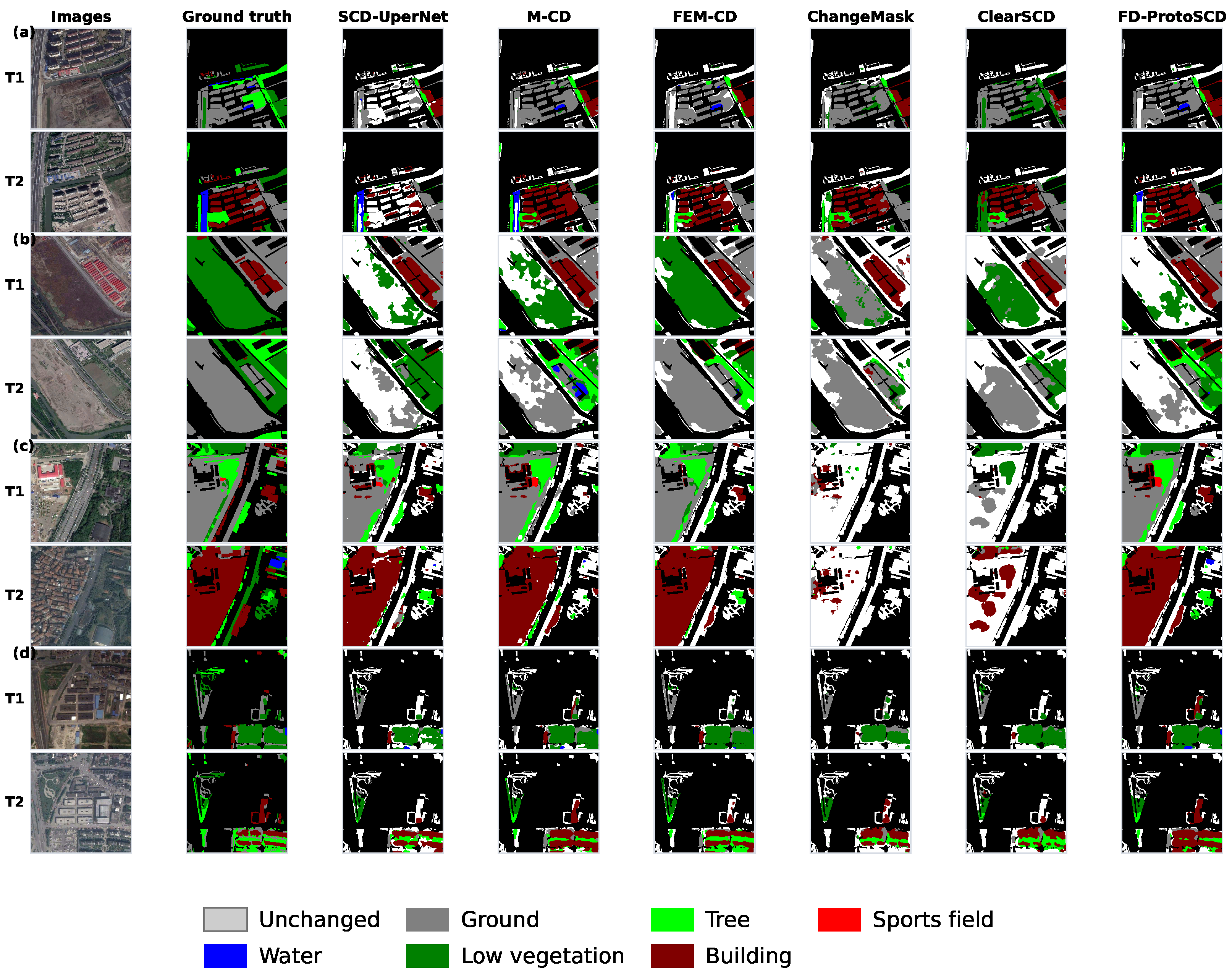
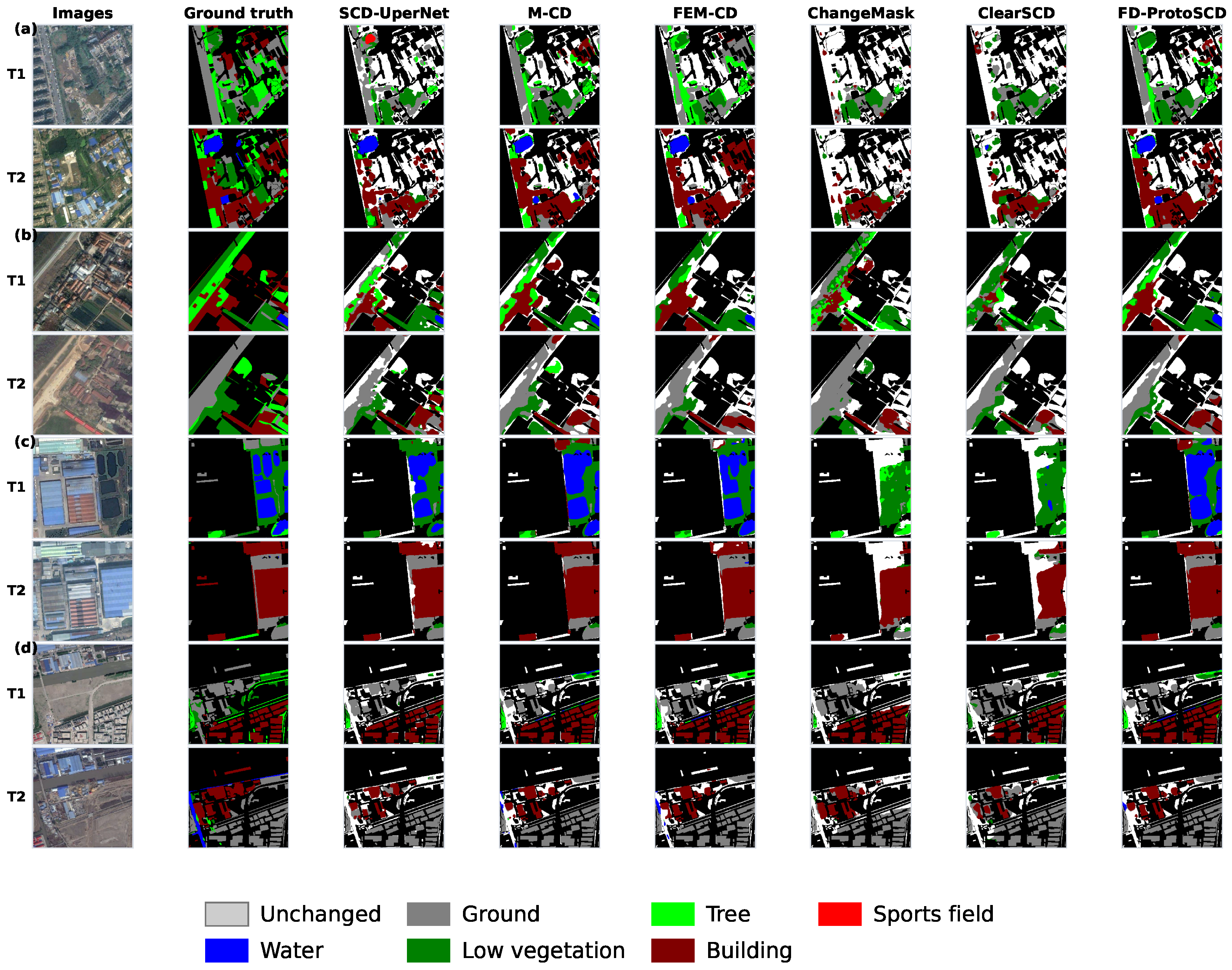
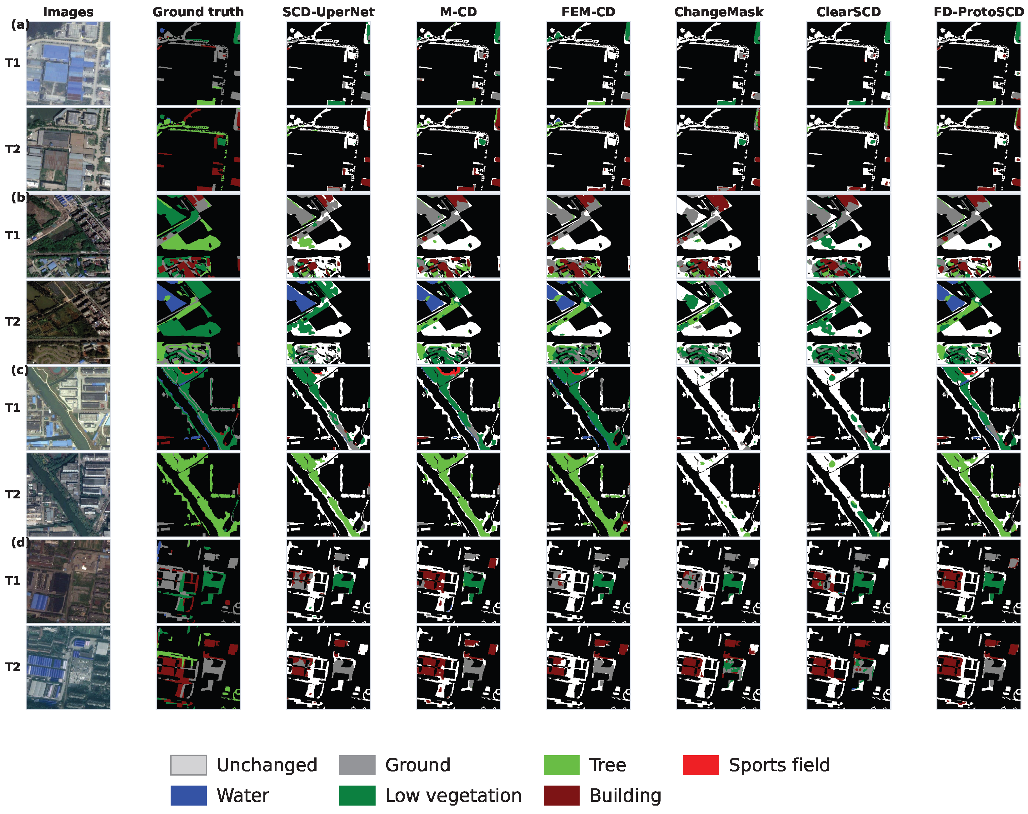
Figure 6, Figure 7, Figure 8 and Figure 9 present sixteen representative SECOND test samples in a ClearSCD-style two-row layout. In response to a reviewer’s suggestion, ChangeMask and ClearSCD are added to the existing SCD-UperNet, M-CD, and FEM-CD comparisons. Each figure therefore aligns the input pair, semantic ground truth, five comparison methods, and FD-ProtoSCD side by side. For ChangeMask and ClearSCD, the displayed outputs average the three checkpoints with the strongest validation semantic performance and fuse their binary-change and semantic heads. All columns use the same modest change-centered crop for each sample to improve the visibility of fine structures without altering the predictions. Across these examples, FD-ProtoSCD produces comparatively compact change regions and preserves several fine structures under illumination and seasonal appearance differences.

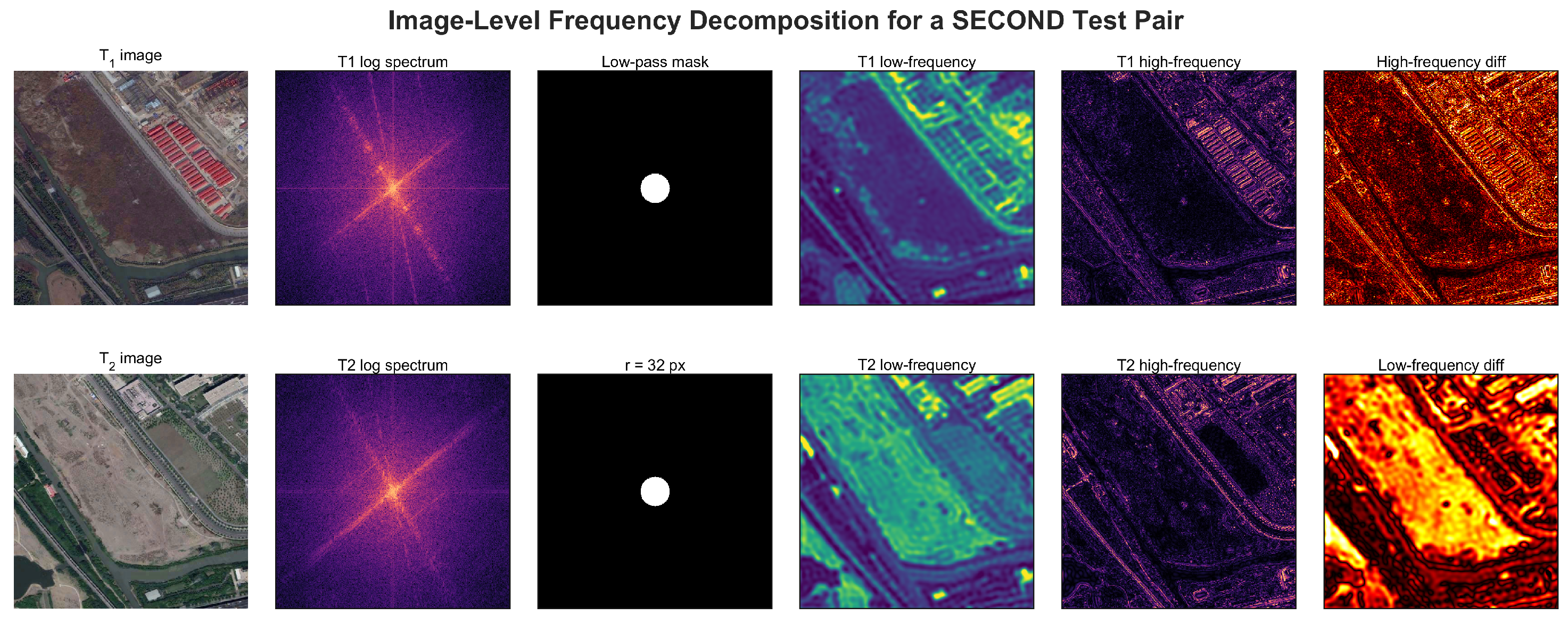
The diagnostic mask uses a radius of 32 pixels in the frequency space. The low-frequency panels preserve broad object layout, while high-frequency panels emphasize edges, texture, and local appearance variation. This image-level example illustrates the spectral motivation for FDCD; because the learned masks operate on multi-scale feature maps, the figure is not presented as direct evidence that every feature-level band has an identical physical meaning.

4.4.2. Frequency Decomposition Visualization

To inspect the frequency content of a representative pair, Figure 10 visualizes an image-level Fourier decomposition with a fixed low-pass radius. This diagnostic shows the frequency structure that directly motivates the FDCD design.

4.4.3. Prototype Transition Analysis

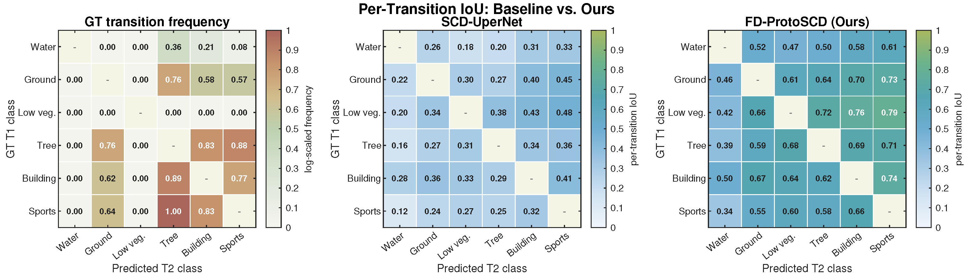
Figure 11 shows the per-transition IoU matrix for SCD-UperNet (baseline) and FD-ProtoSCD on the SECOND test set. Each cell $(i,j)$ gives the IoU of predicting “class j at time $T_2$” conditioned on the ground-truth transition (class $i\to$ class j).

The GT frequency matrix (left) reveals a long-tail distribution: the top 5 transitions dominate the changed pixels. In this diagnostic, FD-ProtoSCD shows higher IoU in several ground-, vegetation-, and sports-field-related cells than SCD-UperNet. The matrix is used to inspect transition-specific behavior; without repeated-run uncertainty, it is not treated as a significance test or as evidence that every rare transition improves uniformly.

4.4.4. False Alarms and Artifact Robustness

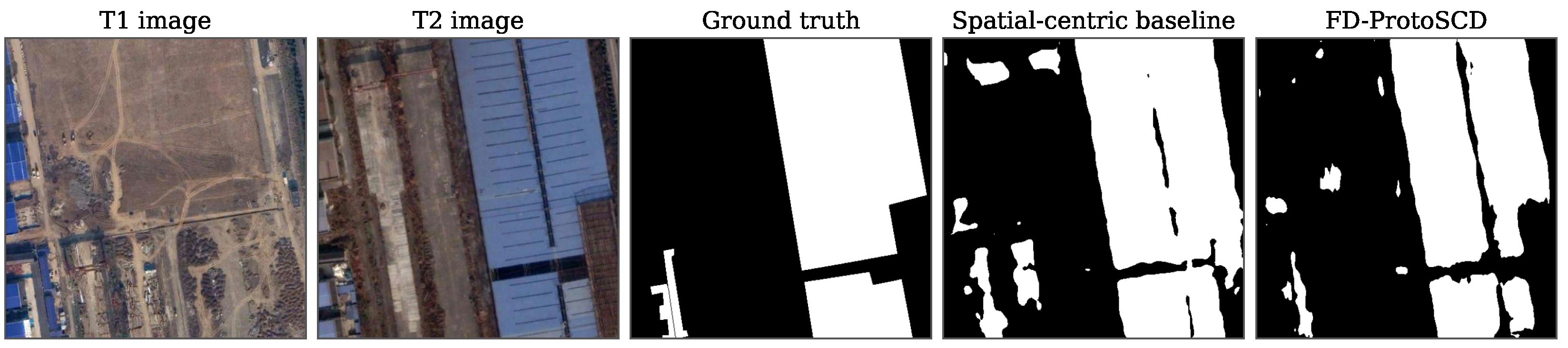
False alarms in change detection correspond to unchanged pixels that are incorrectly classified as changed. They are directly penalized by changed-class Precision and the false positive rate (FPR), whereas F1 and IoU jointly reflect false positives and missed changes. Figure 12 therefore shows the complete, unmasked binary outputs for the same SECOND test pair, rather than displaying predictions only inside the ground-truth change region. On this diagnostic sample, the spatial-centric SCD-UPerNet baseline produces an FPR of 12.63% and a changed-class Recall of 96.24%; FD-ProtoSCD reduces the FPR to 2.97%, with Recall of 90.31%. This example demonstrates suppression of texture-induced responses while also making the associated recall trade-off visible; it is a sample-level diagnostic rather than a substitute for a dedicated corruption benchmark.

The architecture mitigates moderate temporal inconsistency through two model-side mechanisms. First, FDCD computes the principal difference feature from a learned low-frequency branch, while the unchanged-region high-frequency consistency loss discourages texture fluctuations from entering the change signal. Second, the four-level FPN and the unchanged-only placement of this regularizer retain boundary and small-object cues in the semantic heads. These mechanisms are intended to reduce responses to moderate illumination, seasonal texture, contrast, and blur variations, but FD-ProtoSCD does not include explicit radiometric normalization, deblurring, or geometric registration. Severe contrast shifts, blur, atmospheric contamination, or misregistration can therefore still reduce classification accuracy and F1. Because the current benchmarks do not provide controlled corruption annotations, we do not claim invariance or report an unverified corruption score; a severity-controlled corruption benchmark is included in future work. For large scenes, the model can be applied with overlapping sliding-window inference, so images larger than the training crop size can be processed without changing the network architecture.

4.5. Hyperparameter Analysis

4.5.1. Best Settings

Table 5. Selected hyperparameter settings for the reported full model on SECOND.

Group	Best Value	Best ${\mathit{S}}_{\mathit{ek}}$	Source Run
FDCD radius	0.50	24.56	r050
Prototype EMA momentum $\alpha$	0.99	24.56	m099
Pseudo-change loss weight	0.05	24.56	pseudo005
Focal prototype loss weight	0.005	24.56	proto0005

summarizes the best hyperparameter settings used in the full model. The same final configuration appears in several single-factor sweeps because each sweep changes one variable while keeping the remaining selected values fixed; therefore, the repeated best $S_{ek}$ identifies the shared final setting rather than independent claims of different optima.

4.5.2. Sensitivity Analysis

We conducted controlled single-factor hyperparameter studies to confirm the robustness of FD-ProtoSCD against frequency radius, prototype update momentum, and auxiliary loss weights. The primary validation criterion is $S_{ek}$, as it comprehensively checks semantic transition correctness.

The FDCD radius controls the initialization of the soft spectral selector.

Table 6. Sensitivity to FDCD spectral radius on SECOND.

FDCD Radius	Best Iter	$\mathit{F}{1}_{\mathbf{bcd}}$ (%)	${\mathit{S}}_{\mathit{ek}}$	mIoU (%)	Selected
0.10	26 k	72.05	21.61	67.88
0.20	24 k	73.19	22.89	69.66
0.25	29 k	74.04	23.45	71.19
0.35	33 k	74.35	24.02	73.23
0.50	36 k	75.42	24.56	74.85	yes

Bold indicates the best result in each metric column.

reports the observed validation trend within the tested values, with the highest listed score at radius 0.50.

Prototype memory momentum controls structural rigidity during early epochs. Among the tested values in

Table 7. Sensitivity to prototype memory momentum on SECOND.

Setting	Best Iter	$\mathit{F}{1}_{\mathbf{bcd}}$ (%)	${\mathit{S}}_{\mathit{ek}}$	mIoU (%)	Selected
$\alpha =0.90$	30 k	73.85	23.13	71.89
$\alpha =0.95$	29 k	74.89	23.82	72.36
$\alpha =0.99$	36 k	75.42	24.56	74.85	yes
$\alpha =0.995$	31 k	74.15	23.58	71.42

Bold indicates the best result in each metric column.

, $\alpha =0.99$ gives the highest listed validation score.

Auxiliary loss weight balancing confirms that moderate constraints (${\lambda }_{\mathrm{pseudo}}=0.05$ and ${\lambda }_{\mathrm{focal}\text{\_}\mathrm{proto}}=0.005$) yield the sharpest transition mapping in our validation setting. These values are not assumed to be universal constants; for new sensors, resolutions, or annotation policies, they should be re-tuned with a validation set.

Table 8. Sensitivity to auxiliary loss weights on SECOND.

Parameter	Best Iter	$\mathit{F}{1}_{\mathbf{bcd}}$ (%)	${\mathit{S}}_{\mathit{ek}}$	mIoU (%)	Selected
${\lambda }_{\mathrm{pseudo}}=0.00$	27 k	73.57	22.14	68.40
${\lambda }_{\mathrm{pseudo}}=0.025$	30 k	74.45	23.21	71.28
${\lambda }_{\mathrm{pseudo}}=0.05$	36 k	75.42	24.56	74.85	yes
${\lambda }_{\mathrm{pseudo}}=0.10$	32 k	74.81	23.81	73.94
${\lambda }_{\mathrm{focal}\text{\_}\mathrm{proto}}=0.00$	28 k	74.50	23.35	71.75
${\lambda }_{\mathrm{focal}\text{\_}\mathrm{proto}}=0.005$	36 k	75.42	24.56	74.85	yes

Bold indicates the best result in each metric column.

reports the corresponding single-factor loss-weight sweep.

Overall, the tuning results support the component logic of FD-ProtoSCD under the current experimental protocol. Under properly calibrated parameters, the full model achieves the best validation performance among the tested variants.

5. Discussion

5.1. Comparison with Spatial-Centric and Frequency-Aware Paradigms

Conventional spatial-centric SCD models directly compare entangled bi-temporal features. This design is effective when the two images have consistent acquisition conditions, but it can convert illumination, seasonal texture, or atmospheric differences into false change responses. FD-ProtoSCD differs by first separating the difference branch into frequency-aware semantic and appearance components and then decoding the cleaned difference with class prototypes. Figure 1 contrasts the two computational paradigms, Figure 10 visualizes their frequency-domain motivation, and Figure 12 presents their unmasked outputs for the same image pair. Together, these figures show that the spatial-centric path relies on direct feature differencing, whereas our disentangled path uses low-frequency structure to stabilize semantic transition reasoning and regularizes high-frequency residuals in unchanged areas.

At the same time, FDCD should not be interpreted as a generic claim that high-frequency information is useless. The frequency-aliasing, FADC, FreqFusion, FDConv, FDAM, and SFM studies reviewed in Section 2.3 show complementary ways to preserve or adapt high-frequency information in dense prediction [27,28,29,30,31,32]. Our design therefore applies frequency selection only to the change-difference branch, keeps high-frequency information in the encoder and semantic heads, and combines four FPN scales to preserve object structures of different sizes. A same-backbone insertion study with FADC or FreqFusion would be valuable for separating generic frequency enhancement from change-specific disentanglement, but it requires controlled architectural integration and retraining and is outside the experiments completed in this revision.

5.2. Computational Cost and Deployment

FD-ProtoSCD uses 23.92 M parameters. Under our three-run Open-CD benchmark on an NVIDIA RTX 4050 Laptop GPU with batch size 1 and $512\times 512$ inputs, it processes 9.12 image pairs per second. Table 2 reports the same-protocol throughput of locally executable baselines and labels cross-hardware literature values separately. The FDCD module adds FFT/IFFT operations at FPN scales rather than at the original image resolution, and DCPD attends to $2C$ prototypes rather than to all image tokens, limiting the additional memory growth. End-to-end throughput is used as the directly measured cost indicator because common FLOP profilers count complex-valued FFT operations inconsistently across backends; training wall time is likewise affected by validation and checkpoint schedules and is not used for cross-paper ranking. These properties make the model compatible with tiled inference on large remote sensing images, although they do not establish hardware-independent efficiency superiority.

For edge devices such as NVIDIA Jetson, deployment remains unverified. We did not have access to a Jetson platform during this revision, and the FFT/IFFT path still requires platform-specific ONNX/TensorRT compatibility and latency testing. We therefore make no claim of successful Jetson deployment; mixed precision, backend conversion, memory profiling, and sliding-window scheduling are retained as future engineering work.

5.3. Limitations and Future Work

Several limitations remain. First, the FDCD radius initializes the learnable spectral mask and is still selected by validation; future work will develop content-adaptive frequency selection so that the model can adjust spectral bands according to scene type, sensor, and spatial scale. Second, although the low-frequency difference branch reduces sensitivity to spectral noise, severe geometric misregistration can still shift object boundaries and reduce F1. Incorporating explicit image alignment or deformation-aware matching would further improve robustness. A controlled corruption protocol spanning contrast, blur, atmospheric noise, and sub-pixel-to-multi-pixel displacement is also needed to quantify where this mitigation fails. Third, the current Hi-UCD copy available in our workspace supports only binary transfer evaluation, so complete cross-dataset SCD validation requires a version with bi-temporal semantic labels. Fourth, large-scene testing over full 10,000 × 10,000-pixel products should be evaluated with standardized tiling, overlap, and stitching protocols before operational deployment. We did not have a co-registered scene of this size with pixel-level labels matching the present transition taxonomy; an unlabeled stitched visualization would demonstrate executability but would not provide a valid accuracy assessment.

Future work will therefore focus on adaptive spectral selection, deformation-aware temporal alignment, severity-controlled corruption evaluation, richer transition prototypes, and systematic deployment tests on large multi-sensor scenes and edge platforms.

6. Conclusions

This paper addressed two fundamental challenges in Semantic Change Detection for high-resolution remote sensing imagery: pseudo-change contamination caused by illumination and seasonal variation, and severely imbalanced class-transition distributions. We proposed FD-ProtoSCD, a novel multi-task framework that integrates a Frequency-Domain Change Disentanglement (FDCD) module and a Dynamic Class Prototype Decoder (DCPD) into a Siamese encoder–decoder architecture.

The FDCD module uses 2D Fast Fourier Transform and a learnable spectral mask to stabilize semantic change representation, while DCPD uses dynamic prototypes and focal contrastive learning to improve rare transition recognition. Experiments verify that the proposed frequency-prototype paradigm improves semantic consistency and binary change localization across the evaluated SCD and BCD settings. The remaining limitations and future directions, including adaptive frequency selection, geometric alignment, large-scene inference, and edge deployment, are discussed in Section 5.

References

1. Yang, K.; Xia, G.S.; Liu, Z.; Du, B.; Yang, W.; Pelillo, M.; Zhang, L. Asymmetric Siamese Networks for Semantic Change Detection in Aerial Images. IEEE Trans. Geosci. Remote Sens. 2022, 60, 4700718. [Google Scholar] [CrossRef] [Scilit]
2. Chen, H.; Shi, Z. A Spatial-Temporal Attention-Based Method and a New Dataset for Remote Sensing Image Change Detection. Remote Sens. 2020, 12, 1662. [Google Scholar] [CrossRef] [Scilit]
3. Zheng, Z.; Ma, A.; Zhang, L.; Zhong, Y. ChangeMask: Deep Multi-Task Encoder-Transformer-Decoder Architecture for Semantic Change Detection. ISPRS J. Photogramm. Remote Sens. 2022, 183, 228–239. [Google Scholar] [CrossRef] [Scilit]
4. Ding, L.; Guo, H.; Liu, S.; Meng, D.; Zhang, J.; Bruzzone, L. Bi-Temporal Semantic Reasoning for the Semantic Change Detection in HR Remote Sensing Images. IEEE Trans. Geosci. Remote Sens. 2022, 60, 5622214. [Google Scholar] [CrossRef] [Scilit]
5. Tang, K.; Xu, F.; Chen, X.; Dong, Q.; Yuan, Y.; Chen, J. The ClearSCD Model: Comprehensively Leveraging Semantics and Change Relationships for Semantic Change Detection in High Spatial Resolution Remote Sensing Imagery. ISPRS J. Photogramm. Remote Sens. 2024, 211, 299–317. [Google Scholar] [CrossRef] [Scilit]
6. Chen, H.; Qi, Z.; Shi, Z. Remote Sensing Image Change Detection with Transformers. IEEE Trans. Geosci. Remote Sens. 2021, 60, 5607514. [Google Scholar] [CrossRef] [Scilit]
7. Fang, S.; Li, K.; Shao, J.; Li, Z. Changer: Feature Interaction Is What You Need for Change Detection. IEEE Trans. Geosci. Remote Sens. 2023, 61, 5610111. [Google Scholar] [CrossRef] [Scilit]
8. Bandara, W.G.C.; Patel, V.M. A Transformer-Based Siamese Network for Change Detection. In Proceedings of the IEEE International Geoscience and Remote Sensing Symposium (IGARSS), Kuala Lumpur, Malaysia; IEEE: New York, NY, USA, 2022; pp. 207–210. [Google Scholar]
9. Li, Z.; Wang, X.; Fang, S.; Zhao, J.; Yang, S.; Li, W. A Decoder-Focused Multitask Network for Semantic Change Detection. IEEE Trans. Geosci. Remote Sens. 2024, 62, 5609115. [Google Scholar] [CrossRef] [Scilit]
10. Ding, L.; Zhang, J.; Guo, H.; Zhang, K.; Liu, B.; Bruzzone, L. Joint Spatio-Temporal Modeling for Semantic Change Detection in Remote Sensing Images. IEEE Trans. Geosci. Remote Sens. 2024, 62, 5610814. [Google Scholar] [CrossRef] [Scilit]
11. Long, J.; Li, M.; Wang, X.; Stein, A. Semantic Change Detection Using a Hierarchical Semantic Graph Interaction Network from High-Resolution Remote Sensing Images. ISPRS J. Photogramm. Remote Sens. 2024, 211, 318–335. [Google Scholar] [CrossRef] [Scilit]
12. Mei, L.; Ye, Z.; Xu, C.; Wang, H.; Wang, Y.; Lei, C.; Yang, W.; Li, Y. SCD-SAM: Adapting Segment Anything Model for Semantic Change Detection in Remote Sensing Imagery. IEEE Trans. Geosci. Remote Sens. 2024, 62, 5626713. [Google Scholar] [CrossRef] [Scilit]
13. Stephen, A.; Zhou, X.; Wang, Z.; Dong, P.; Li, W. TripleS: Mitigating Multi-Task Learning Conflicts for Semantic Change Detection in High-Resolution Remote Sensing Imagery. ISPRS J. Photogramm. Remote Sens. 2025, 222, 91–108. [Google Scholar] [CrossRef] [Scilit]
14. Long, J.; Zeng, H.; Zhao, H.; Lin, H.; Li, J. Detecting Semantic Changes from VHR Remote Sensing Images by Integrating Semantic Correlations and Change Priors. Int. J. Appl. Earth Obs. Geoinf. 2025, 144, 104916. [Google Scholar] [CrossRef] [Scilit]
15. Long, J.; Liu, S.; Li, M.; Zhao, H.; Jin, Y. BGSNet: A Boundary-Guided Siamese Multitask Network for Semantic Change Detection from High-Resolution Remote Sensing Images. ISPRS J. Photogramm. Remote Sens. 2025, 225, 221–237. [Google Scholar] [CrossRef] [Scilit]
16. Jiang, Z.; Wang, B.; Zhang, P.; Wu, Y.; Ye, Z.; Yang, H. Semantic Enhancement and Change Consistency Network for Semantic Change Detection in Remote Sensing Images. Int. J. Digit. Earth 2025, 18, 2496790. [Google Scholar] [CrossRef] [Scilit]
17. Qu, Y.; Li, J.; Pan, X.; Huang, X. S3CD: A Self-Supervised Semantic Change Detection Method by Mining Transition Patterns and Consistency in Remote Sensing Images. IEEE Trans. Cybern. 2026, 56, 1452–1464. [Google Scholar] [CrossRef] [Scilit] [PubMed]
18. Daudt, R.C.; Le Saux, B.; Boulch, A. Fully Convolutional Siamese Networks for Change Detection. In Proceedings of the IEEE International Conference on Image Processing (ICIP), Athens, Greece; IEEE: New York, NY, USA, 2018; pp. 4063–4067. [Google Scholar]
19. Chen, H.; Song, J.; Han, C.; Shi, Z. ChangeMamba: Remote Sensing Change Detection with Spatiotemporal State Space Model. IEEE Trans. Geosci. Remote Sens. 2024, 62, 5626514. [Google Scholar] [CrossRef] [Scilit]
20. Wang, Q.; Jing, W.; Chi, K.; Yuan, Y. Cross-Difference Semantic Consistency Network for Semantic Change Detection. IEEE Trans. Geosci. Remote Sens. 2024, 62, 4406312. [Google Scholar] [CrossRef] [Scilit]
21. Wang, B.; Jiang, Z.; Ma, W.; Xu, X.; Zhang, P.; Wu, Y.; Yang, H. Dual-Dimension Feature Interaction for Semantic Change Detection in Remote Sensing Images. IEEE J. Sel. Top. Appl. Earth Obs. Remote Sens. 2024, 17, 9595–9605. [Google Scholar] [CrossRef] [Scilit]
22. Ning, X.; He, Y.; Zhang, H.; Zhang, R.; Chang, D.; Hao, M. Semantic Information Collaboration Network for Semantic Change Detection in Remote Sensing Images. IEEE J. Sel. Top. Appl. Earth Obs. Remote Sens. 2024, 17, 12893–12909. [Google Scholar] [CrossRef] [Scilit]
23. Tan, L.; Zuo, X.; Cheng, X. CGMNet: Semantic Change Detection via a Change-Aware Guided Multi-Task Network. Remote Sens. 2024, 16, 2436. [Google Scholar] [CrossRef] [Scilit]
24. Ding, Q.; Shao, Z.; Huang, X.; Wang, F.; Wang, M. MLFA-Net: Multi-Level Feature-Aggregated Network for Semantic Change Detection in Remote Sensing Images. Int. J. Digit. Earth 2024, 17, 2398070. [Google Scholar] [CrossRef] [Scilit]
25. Yang, Y.; Soatto, S. FDA: Fourier Domain Adaptation for Semantic Segmentation. In Proceedings of the IEEE/CVF Conference on Computer Vision and Pattern Recognition (CVPR); IEEE: New York, NY, USA, 2020; pp. 4084–4094. [Google Scholar] [CrossRef] [Scilit]
26. Chi, L.; Jiang, B.; Mu, Y. Fast Fourier Convolution. In Proceedings of the Advances in Neural Information Processing Systems (NeurIPS); NeurIPS: San Diego, CA, USA, 2020; Volume 33, pp. 4479–4488. [Google Scholar]
27. Chen, L.; Gu, L.; Fu, Y. When Semantic Segmentation Meets Frequency Aliasing. In Proceedings of the International Conference on Learning Representations (ICLR); ICLR: Appleton, WI, USA, 2024. [Google Scholar]
28. Chen, L.; Gu, L.; Zheng, D.; Fu, Y. Frequency-Adaptive Dilated Convolution for Semantic Segmentation. In Proceedings of the IEEE/CVF Conference on Computer Vision and Pattern Recognition (CVPR); IEEE: New York, NY, USA, 2024; pp. 3414–3425. [Google Scholar] [CrossRef] [Scilit]
29. Chen, L.; Fu, Y.; Gu, L.; Yan, C.; Harada, T.; Huang, G. Frequency-Aware Feature Fusion for Dense Image Prediction. IEEE Trans. Pattern Anal. Mach. Intell. 2024, 46, 10763–10780. [Google Scholar] [CrossRef] [Scilit] [PubMed]
30. Chen, L.; Gu, L.; Li, L.; Yan, C.; Fu, Y. Frequency Dynamic Convolution for Dense Image Prediction. In Proceedings of the IEEE/CVF Conference on Computer Vision and Pattern Recognition (CVPR); IEEE: New York, NY, USA, 2025; pp. 30178–30188. [Google Scholar] [CrossRef] [Scilit]
31. Chen, L.; Gu, L.; Fu, Y. Frequency-Dynamic Attention Modulation for Dense Prediction. In Proceedings of the IEEE/CVF International Conference on Computer Vision (ICCV); IEEE: New York, NY, USA, 2025; pp. 22620–22632. [Google Scholar] [CrossRef] [Scilit]
32. Chen, L.; Fu, Y.; Gu, L.; Zheng, D.; Dai, J. Spatial Frequency Modulation for Semantic Segmentation. IEEE Trans. Pattern Anal. Mach. Intell. 2025, 47, 9767–9784. [Google Scholar] [CrossRef] [Scilit] [PubMed]
33. Wang, D.; Zhuang, L.; Gao, L.; Sun, X.; Zhao, X. Global Feature-Injected Blind-Spot Network for Hyperspectral Anomaly Detection. IEEE Geosci. Remote Sens. Lett. 2024, 21, 5509305. [Google Scholar] [CrossRef] [Scilit]
34. Wang, Y.; Zheng, H.; Li, F.; Lin, Y.; Fan, L.; He, X.; Huang, Y.; Ding, X. Toward Generalizable Pansharpening: Conditional Flow-Based Learning Guided by Implicit High-Frequency Priors. IEEE Trans. Geosci. Remote Sens. 2025, 63, 5401917. [Google Scholar] [CrossRef] [Scilit]
35. Wang, D.; Gao, L.; Qu, Y.; Sun, X.; Liao, W. Frequency-to-Spectrum Mapping GAN for Semisupervised Hyperspectral Anomaly Detection. CAAI Trans. Intell. Technol. 2023, 8, 1258–1273. [Google Scholar] [CrossRef] [Scilit]
36. Zang, Q.; Zhao, D.; Wang, S.; Quan, D.; Zhong, Z. Feature Spectrum Learning for Remote Sensing Change Detection. In Proceedings of the IEEE/CVF Conference on Computer Vision and Pattern Recognition (CVPR); IEEE: New York, NY, USA, 2025; pp. 12647–12657. [Google Scholar] [CrossRef] [Scilit]
37. Zhu, T.; Zhao, Z.; Xia, M.; Huang, J.; Weng, L. FTA-Net: Frequency-Temporal-Aware Network for Remote Sensing Change Detection. IEEE J. Sel. Top. Appl. Earth Obs. Remote Sens. 2025, 18, 3448–3460. [Google Scholar] [CrossRef] [Scilit]
38. Xing, Y.; Jia, Y.; Gao, S.; Hu, J.; Huang, R. Frequency-Enhanced Mamba for Remote Sensing Change Detection. IEEE Geosci. Remote Sens. Lett. 2025, 22, 8003305. [Google Scholar] [CrossRef] [Scilit]
39. Zhao, L.; Zhao, C.; Zhang, L.; Zhong, Z. FACDNet: A Frequency-Aware Cross-Layer Network for Remote Sensing Change Detection. Electronics 2026, 15, 2416. [Google Scholar] [CrossRef] [Scilit]
40. Snell, J.; Swersky, K.; Zemel, R. Prototypical Networks for Few-Shot Learning. In Proceedings of the Advances in Neural Information Processing Systems (NeurIPS); NeurIPS: San Diego, CA, USA, 2017; Volume 30. [Google Scholar]
41. Wang, K.; Liew, J.H.; Zou, Y.; Zhou, D.; Feng, J. PANet: Few-Shot Image Semantic Segmentation with Prototype Alignment. In Proceedings of the IEEE/CVF International Conference on Computer Vision (ICCV); IEEE: New York, NY, USA, 2019; pp. 9197–9206. [Google Scholar] [CrossRef] [Scilit]
42. Shen, W.; Ma, A.; Wang, J.; Zheng, Z.; Zhong, Y. Adaptive Self-Supporting Prototype Learning for Remote Sensing Few-Shot Semantic Segmentation. IEEE Trans. Geosci. Remote Sens. 2024, 62, 5910216. [Google Scholar] [CrossRef] [Scilit]
43. Fang, S.; Li, W.; Song, Y.; Li, Z.; Zhao, J. Rethinking Semantic Change Detection from a Semantic Alignment Perspective. IEEE Trans. Geosci. Remote Sens. 2025, 63, 4417215. [Google Scholar] [CrossRef] [Scilit]
44. Gao, Y.; Li, T.; Wang, K.; Wang, G.; Ma, J. Integrating Semisupervision and Prototype Contrastive Learning for Robust Semantic Change Detection in Remote Sensing Images. IEEE Trans. Geosci. Remote Sens. 2026, 64, 5601217. [Google Scholar] [CrossRef] [Scilit]
45. Tian, T.; Li, C.; Qing, Y.; Cheng, S. Hi-UCD: A Large-Scale Dataset for Urban Semantic Change Detection in Remote Sensing Imagery. arXiv 2020, arXiv:2011.03247. [Google Scholar]
46. Li, K.; Fang, S.; Li, H.; He, Z. Open-CD: A Comprehensive Toolbox for Change Detection. arXiv 2024, arXiv:2407.15317. [Google Scholar]
47. Li, C.; Shen, R.; Li, J.; Wang, B. SNUNet-CD: A Densely Connected Siamese Network for Change Detection of VHR Images. IEEE Geosci. Remote Sens. Lett. 2021, 19, 8007805. [Google Scholar] [CrossRef] [Scilit]
48. Mou, L.; Bruzzone, L.; Zhu, X.X. Learning Spectral-Spatial-Temporal Features via a Recurrent Convolutional Neural Network for Change Detection in Multispectral Imagery. IEEE Trans. Geosci. Remote Sens. 2019, 57, 924–935. [Google Scholar] [CrossRef] [Scilit]
49. Daudt, R.C.; Le Saux, B.; Boulch, A.; Gousseau, Y. Multitask Learning for Large-Scale Semantic Change Detection. Comput. Vis. Image Underst. 2019, 187, 102783. [Google Scholar] [CrossRef] [Scilit]
50. Peng, D.; Bruzzone, L.; Zhang, Y.; Guan, H.; He, P. SCDNET: A Novel Convolutional Network for Semantic Change Detection in High Resolution Optical Remote Sensing Imagery. Int. J. Appl. Earth Obs. Geoinf. 2021, 103, 102465. [Google Scholar] [CrossRef] [Scilit]
51. Paranjape, J.N.; De Melo, C.; Patel, V.M. A Mamba-Based Siamese Network for Remote Sensing Change Detection. In Proceedings of the IEEE/CVF Winter Conference on Applications of Computer Vision (WACV), Tucson, AZ, USA; IEEE: New York, NY, USA, 2025; pp. 1186–1196. [Google Scholar]
52. Liu, X.; Dai, C.; Ding, L.; Zhang, Z.; Li, Y.; Zuo, X.; Li, M.; Wang, H.; Miao, Y. GSTM-SCD: Graph-Enhanced Spatio-Temporal State Space Model for Semantic Change Detection in Multi-Temporal Remote Sensing Images. ISPRS J. Photogramm. Remote Sens. 2025, 230, 73–91. [Google Scholar] [CrossRef] [Scilit]
Figure 1. Comparison of representative change detection frameworks and FD-ProtoSCD. Solid arrows indicate the main prediction flow, while dotted/dashed arrows denote feature interaction or auxiliary guidance paths. Colored blocks distinguish inputs, encoders, decoders, priors/prototypes, and output maps as labeled in the figure.
Remotesensing 18 02957 g001
Figure 2. Motivation of FD-ProtoSCD. (a) Pseudo-change interference from high-frequency appearance shifts. (b) Long-tailed transition distribution and target-class IoU on SECOND.
Remotesensing 18 02957 g002
Figure 3. Overall architecture of FD-ProtoSCD. The Siamese encoder extracts multi-scale features from bi-temporal images; FDCD modules disentangle semantic differences from pseudo-changes in the frequency domain; the DCPD decoder performs focal-re-weighted prototype cross-attention; three output heads produce the binary change mask and the pre-/post-change semantic maps. Solid arrows show feature and prediction flow, while dashed or dotted arrows indicate supervision and auxiliary loss paths. Colored blocks distinguish the encoder, FPN aggregation, FDCD, DCPD, semantic heads, binary head, ground truths, and loss terms.
Remotesensing 18 02957 g003
Figure 4. Detailed architecture of the Frequency-Domain Change Disentanglement (FDCD) module. The module applies 2D Fast Fourier Transform to bi-temporal feature maps, yielding frequency spectra that are separated by a learnable mask into low-frequency semantics and high-frequency appearances. Arrows show the FFT-based decomposition and feature-difference flow; colored branches distinguish the low-frequency semantic path, high-frequency appearance path, and auxiliary pseudo-change loss. Differences in the semantic subspace highlight genuine context changes, while variations in the appearance subspace are constrained by a pseudo-change suppression loss to eliminate seasonal or lighting artifacts.
Remotesensing 18 02957 g004
Figure 5. Structure of the Dynamic Class Prototype Decoder (DCPD). Using the semantic difference features from FDCD as queries, the module applies dual-prototype cross-attention against the continuously updated semantic prototype banks of both temporal branches. Arrows denote feature, prototype-update, and attention flows; colored blocks distinguish prototype memory, attention, feed-forward decoding, and focal contrastive supervision. This explicitly guides the decoder to focus on specific land-cover transitions and relies on a focal contrastive loss to mitigate the class imbalance problem by re-weighting gradients for rare transitions.
Remotesensing 18 02957 g005
Figure 6. Qualitative comparison on SECOND, group 1. Subfigures (ad) show four representative T1/T2 sample pairs. In each subfigure, rows are arranged as T1/T2 pairs; columns show the input images, semantic ground truth, SCD-UperNet, M-CD, FEM-CD, ChangeMask, ClearSCD, and FD-ProtoSCD.
Remotesensing 18 02957 g006
Figure 7. Qualitative comparison on SECOND, group 2. Subfigures (ad) show four additional T1/T2 sample pairs. The layout is identical to Figure 6, so the methods can be compared across different transition patterns without re-learning the legend.
Remotesensing 18 02957 g007
Figure 8. Qualitative comparison on SECOND, group 3. Subfigures (ad) show four T1/T2 sample pairs. This set emphasizes small and mixed transitions where semantic confusion is easy to spot.
Remotesensing 18 02957 g008
Figure 9. Qualitative comparison on SECOND, group 4. Subfigures (ad) show four T1/T2 sample pairs. The final set collects the hardest remaining examples, so the comparison includes both sparse change regions and more fragmented structures.
Remotesensing 18 02957 g009
Figure 10. Image-level frequency decomposition for one SECOND test pair. Top row (T1): input image, log-magnitude spectrum, fixed low-pass mask, low-frequency reconstruction, high-frequency residual, and high-frequency difference. Bottom row (T2): same decomposition, with the final cell showing the low-frequency difference. RGB panels use the original remote sensing colors; spectrum panels use the displayed color scale to show log-magnitude intensity; white regions in the mask denote retained low-frequency components and black regions denote suppressed high-frequency components.
Remotesensing 18 02957 g010
Figure 11. Per-transition IoU matrices and GT transition frequency. Left: ground-truth transition pixel frequency (log scale). Center: SCD-UperNet per-transition IoU. Right: FD-ProtoSCD per-transition IoU. The matrices provide a transition-level diagnostic of how the two models distribute their correct predictions.
Remotesensing 18 02957 g011
Figure 12. Unmasked output comparison on a representative SECOND test pair. White denotes predicted change and black denotes unchanged pixels in the last three panels. The final two panels are the requested outputs from a conventional spatial-centric SCD-UPerNet baseline and the proposed frequency-disentangled/prototype-guided paradigm, respectively. No ground-truth mask is applied to either prediction, so false alarms remain visible.
Remotesensing 18 02957 g012