A Change-Point-Based Deformation Grouping Strategy in Long-Term Near-Real-Time Deformation Monitoring

Highlights

What are the main findings?

• We propose a Change-Point-Based Deformation Grouping Strategy that balances computational efficiency and deformation estimation accuracy by constraining group size and determining grouping boundaries based on detected deformation change points.
• By combining a Bidirectional LSTM network with the Bayesian Estimator of Abrupt Change, Seasonality and Trend (BEAST), the proposed method improves robustness compared with conventional change point detection methods.

What are the implications of the main findings?

• This study demonstrates that integrating deep learning models (Bidirectional LSTM) with statistical algorithms (BEAST) to detect abrupt deformation change points enables a more scientifically grounded data grouping strategy.
• By grouping observations with consistent deformation characteristics, the method reduces the risk of smoothing over abrupt deformation changes. This directly provides reliable deformation estimates and enables robust analysis of abrupt ground deformation events, which are often the most critical for hazard assessment.

Abstract

Distributed Scatterer Interferometric Synthetic Aperture Radar (DSInSAR) technology has been widely applied in areas with complex terrain and dense vegetation. However, DSInSAR is computationally intensive and requires considerable processing time. When new observations become available, the entire dataset must be reprocessed without utilizing previously obtained results. This makes DSInSAR unsuitable for long-term continuous monitoring. The Sequential Estimator partitions large datasets into fixed-size subsets and compresses these subsets to avoid redundant processing. The Recursive Sequential Estimator with Flexible Batches (RSEFB) method was proposed to partition large datasets into flexibly sized subsets. However, how to determine appropriate grouping boundaries remains unresolved. In this paper, a Change-Point-Based Deformation Grouping Strategy (CPDGS) is proposed to enhance the deformation estimation accuracy within each group, thereby reducing the attenuation of abrupt deformation signals during estimation. In the proposed method, a Bidirectional Long Short-Term Memory (Bidirectional LSTM) network is employed to identify the potential presence of deformation change points. Bayesian Estimator of Abrupt change, Seasonality and Trend (BEAST) is subsequently used to localize the change points. Considering computational efficiency, an upper limit is also set on the number of Single Look Complex (SLC) per group. Due to the lack of ground truth, simulated data were used for the network training. Comparative experiments show that the proposed Bidirectional LSTM achieves the best overall performance, with an accuracy of 88.43%, a precision of 90.76%, a recall of 86.04%, and an F1-score of 88.34%, outperforming the LSTM and Transformer models. Further comparisons with conventional change point detection methods show that the proposed method achieves an F1-score of 91.23%, higher than Cumulative Sum (CUSUM; 69.20%) and and Bayesian Online Change Point Detection (BOCPD; 84.44%). Experiments using real Interferometric Synthetic Aperture Radar (InSAR) deformation data further demonstrate its effectiveness in identifying deformation change points in practical scenarios.

1. Introduction

Surface deformation, commonly manifested as subsidence or uplift, is closely associated with various geohazards, including landslides, ground fissures and land subsidence [1]. Surface deformation is a long-standing geo-environmental problem prevalent across numerous regions worldwide. Achieving long-term, high-precision monitoring is important for ensuring the safe operation of urban infrastructure [2,3].

Traditional deformation monitoring techniques, such as the Global Navigation Satellite System (GNSS) [4], provide high-accuracy point measurements but have limited spatial coverage. However, due to the high deployment costs, these methods cannot readily provide spatially continuous deformation measurements over large areas at high spatial resolution. In the past 20 years, Interferometric Synthetic Aperture Radar (InSAR) has become a core technique for large-area ground deformation monitoring, benefiting from its all-weather, all-day, and large-scale observation capabilities [5]. Accordingly, it has become a core tool for monitoring various geological hazards and geodynamic activities, such as landslides [6], mining deformation [6], volcanism [7], urban subsidence [8] and infrastructure displacement [9,10,11]. Time Series Interferometric Synthetic Aperture Radar (TSInSAR) has become an effective remote sensing technique that utilizes the phase information from a series of synthetic aperture radar (SAR) images to monitor deformation [12]. To overcome the temporal decorrelation and the atmospheric phase screen (APS) [13], Persistent Scatterers Interferometric Synthetic Aperture Radar (PSInSAR) [14] was proposed. PSInSAR exploits scatterers that remain phase-stable throughout the observation period. However, only a limited number of persistent scatterers can be identified. The low density of persistent scatterers not only complicates subsequent phase unwrapping but also increases uncertainty in deformation estimation [15]. To monitor deformation in mountainous regions, the Small Baseline Subset (SBAS) technology has rapidly developed. By limiting the length of spatiotemporal baselines, SBAS avoids spatiotemporal decoherence of measurement points [16]. To jointly exploit persistent scatterers (PS) and distributed scatterers (DS), Ferretti et al. proposed SqueeSAR [17]. Despite its wide spatial coverage and high deformation estimation accuracy, SqueeSAR is computationally demanding. This makes SqueeSAR unsuitable for long-term continuous monitoring [18].

To make SqueeSAR available for long-term deformation monitoring, near-real-time InSAR (NRT InSAR) was proposed to avoid redundant processing [19]. The Sequential Estimator (SE) was proposed by Ansari et al. [20], which partitions large datasets into fixed-size subsets and compresses these subsets to avoid redundant processing. The algorithm has become a critical foundational component for NRT InSAR. Wang et al. combined the sequential least squares and SBAS to propose the sequential SBAS algorithm, which enables dynamic integration of newly acquired data into its processed data [21]. Ma et al. combined the Sequential Estimator, azimuth deformation estimation and Sentinel-1 data co-registration [22]. The Recursive Sequential Estimator with Flexible Batches (RSEFB) was proposed to relax the number of images in each subset [23].

However, an important issue remains unresolved in existing Sequential-Estimator-based NRT InSAR methods: how to determine appropriate grouping boundaries while maintaining both computational efficiency and deformation estimation accuracy. SE generally adopts fixed-size grouping, which may cause deformation change points to occur within the group and consequently reduce the accuracy of intra-group deformation estimation. Although RSEFB allows flexible group sizes, it does not provide a systematic criterion for determining grouping boundaries. Therefore, an adaptive grouping strategy driven by deformation characteristics is still required.

To address this issue, this study proposes a Change-Point-Based Deformation Grouping Strategy (CPDGS) for long-term NRT InSAR monitoring. The main contributions are summarized as follows:

• A deformation-driven grouping strategy is proposed, in which deformation change points are used to determine grouping boundaries instead of relying solely on fixed-size grouping.
• A change-point detection framework combining Bidirectional Long Short-Term Memory (Bidirectional LSTM)and Bayesian Estimator of Abrupt change, Seasonality, and Trend (BEAST) is developed. The two methods perform complementary functions: Bidirectional LSTM determines whether a deformation sequence contains a change point, while BEAST subsequently determines the location of the change point. This combination improves the robustness of change point detection under noisy deformation observations.

2. Related Works

2.1. SqueeSAR

Distributed scatterers (DSs) are characterized by the presence of multiple scattering sources within a pixel, whereas persistent scatterers (PSs) are defined by a single dominant scatterer within a resolution cell [17]. SqueeSAR jointly processes persistent scatterer (PS) and distributed scatterer (DS) targets. DS targets generally exhibit lower phase stability than PS targets. Therefore, the phase information of DS targets generally requires additional processing, such as multilooking or phase filtering, before it can be used for deformation monitoring [24].

SqueeSAR enhances the coherence and phase quality of distributed scatterers by utilizing the statistical homogeneity of the DS targets. Distributed Scatterers Interferometric Synthetic Aperture Radar (PSInSAR)primarily relies on identifying statistically homogeneous pixels (SHPs) and applying phase linking to improve the phase stability of distributed scatterers [25].

The SHPs refer to the pixels that have the same amplitude distribution as the reference pixel. SHPs are neighboring pixels whose amplitude statistics are consistent with those of the reference pixel [26].

The interferometric information from the fully connected network can be represented by the coherence matrix constructed from the SHPs.

$$\Gamma (p)={\displaystyle \frac{1}{\left|\Omega \right|}}{\displaystyle \sum _{p\in \Omega }d}(p)\cdot d{\left(p\right)}^{\mathrm{H}}$$

(1)

where $d$ is the normalized complex reflectivity vector, $\mathrm{H}$ is the Hermitian transpose, $p$ is the pixel of the SAR image, $\Omega$ is the SHP, $\Gamma$ is the coherence matrix, and $\left|\Omega \right|$ denotes the number of pixels within the statistically homogeneous pixel (SHP).

Phase quality can be improved through maximum-likelihood estimation based on the coherence matrix, a procedure commonly referred to as phase linking [27].

$${\widehat{\theta }}_n^k=\arg \left\{{\displaystyle {\displaystyle \sum _{m\ne n}^N}{\left\{|\Gamma {|}^{-1}\right\}}_{mn}}{\left\{\Gamma \right\}}_{mn}\exp (j{\widehat{\theta }}_m^{k-1})\right\}$$

(2)

where $k$ is the iteration step, ${\widehat{\theta }}_n^k$ is the phase estimate obtained at iteration $k$, $N$ is the number of SAR images, $m,n$ is the SAR image index, $j$ is the imaginary unit, and $\theta ={[{\theta }_1,{\theta }_2,\dots ,{\theta }_N]}^{\mathrm{T}}$ is the optimal phase series.

After phase linking, the phase stability of the processed DS targets becomes comparable to that of PS targets [28]. It should be noted that the coherence matrix is an $N\times N$ matrix, where $N$ represents the number of Single Look Complex (SLC) images in the dataset and a coherence matrix is constructed for each pixel. The computational cost of forming and processing the full coherence matrix makes conventional DSInSAR processing increasingly demanding for long-term monitoring, particularly when newly acquired SAR images must be processed sequentially [17].

2.2. NRT InSAR

Short-Revisit Synthetic Aperture Radar satellites provide a large amount of data for InSAR deformation monitoring, which makes long-term continuous deformation monitoring possible. However, the rapidly increasing data volume also places greater demands on sequential processing methods that can incorporate newly acquired observations without reprocessing previously processed data [20].

2.2.1. Sequential Estimator

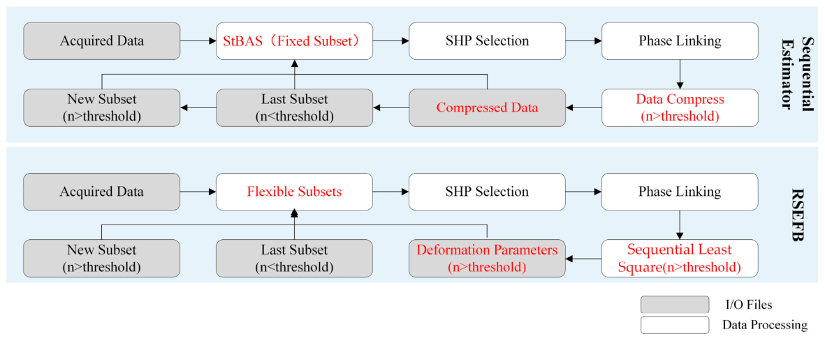
SE was proposed by Ansari et al. to divide the dataset into small batches with a fixed number of SAR images, which is called Small Temporal Baseline Subset (StBAS) [20]. As shown in Figure 1, in each batch, Maximum Likelihood Estimation phase linking is applied to extract the optimal phase series. When the number of SAR images in a batch reaches a predefined threshold, SE performs compression on these batches along the time dimension. The core idea of SE is to jointly process compressed historical data and newly acquired observations, thereby preserving long-term coherence information while improving deformation estimation within short-temporal-baseline subsets.

During NRT deformation monitoring using SE, the size of the newly acquired SLC chunk expands from 1 to s − 1, triggering the immediate application of phase linking and SqueeSAR to each new SLC acquisition. Data compression is triggered when the temporal baseline exceeds a predefined threshold [20].

2.2.2. Recursive Sequential Estimator with Flexible Batches (RSEFB)

Building on SE and sequential least-squares estimation, the Recursive Sequential Estimator with Flexible Batches (RSEFB) partitions large datasets into flexibly sized batches without imposing a fixed number of images per batch [22].

RSEFB divides the already acquired data into k flexibly sized batches. The head-to-tail connection mode is employed to facilitate the linking of all subsets, implying that the last image of the preceding batch is also the first image of the subsequent batch, instead of using compressed data as in SE. This scheme preserves continuity between adjacent subsets.

For near-real-time deformation monitoring, RSEFB uses sequential least-squares estimation to recursively update the deformation parameters across successive batches. The optimal initial estimation of the second batch is derived from the adjusted result of the first batch, and then the optimal initial estimation of the third batch is derived from the integration of the previous two. In this way, all the batches are connected recursively [22].

The observation equation and the recursive equation for batches 1 and 2 can be expressed as

$${\theta }_1=A_1{X}_1+{\Delta }_1,P_1$$

(3)

$${\theta }_2=A_2{X}_2+{\Delta }_2,P_2$$

(4)

where ${\theta }_1,{\theta }_2$ are the optimal sequential phases in groups 1 and 2, $X_1$, $X_2$ are the parameters vectors of time series deformation in groups 1 and 2, $A_1$ and $A_2$ are the coefficient matrixes, ${\Delta }_1$ and ${\Delta }_2$ are the noise vectors, and $P_1,P_2$ are the covariance matrixes of the parameter estimation error in groups 1 and 2.

Let $Q_{X_1}$ be the covariance matrix of $X_1$:

$${\widehat{X}}_1={\left(\begin{array}{c}{A}_1^T{P}_1{A}_1\end{array}\right)}^{-1}{A}_1^{T}P{\theta }_1$$

(5)

$$Q_{X_1}={\left(A_1^T{P}_1{A}_1\right)}^{-1}$$

(6)

The covariance matrix of $X_2$ is $Q_{X_2}$:

$${\widehat{X}}_2={\widehat{X}}_1+J_k({\theta }_2-A_2{\widehat{X}}_1)$$

(7)

$$Q_{X_2}=Q_{X_1}-J_k{A}_2{Q}_{X_1}$$

(8)

The gain matrix $J_k$ is:

$$J_k=Q_{X_1}{A}_2^{\mathrm{T}}{\left(P_2^{-1}+A_2{Q}_{X_1}{A}_2^{\mathrm{T}}\right)}^{-1}$$

(9)

where ${\widehat{X}}_1,{\widehat{X}}_2$ are the estimated deformation parameter vectors of groups 1 and 2.

As highlighted in Figure 1, RSEFB relaxes the requirements on the number of images compared to StBAS, but it does not specify a systematic grouping methodology; it merely references manual grouping depending on seasonal patterns or the coherence matrix.

3. Methodology

Appropriate data grouping is crucial in both SE and RSEFB; however, neither method provides a systematic criterion for determining grouping boundaries. SE employs StBAS as the strategy for grouping, which leads to a fixed number stack; RSEFB relaxes the fixed-size constraint, but does not specify how the grouping boundaries should be determined. In this study, we propose a Change-Point-Based Deformation Grouping Strategy to enhance the accuracy of deformation estimation within each group, thereby improving the overall deformation estimation accuracy, particularly for long-term deformation monitoring applications. Considering the computational efficiency of SqueeSAR, an upper limit on the number of SLCs per group is also set. In this section, we present a complete workflow of the proposed grouping strategy.

3.1. Initial Processing

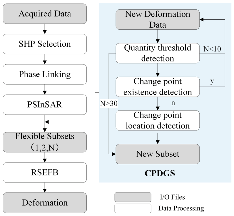
For the data available before the initial processing, we use SqueeSAR and PSInSAR to derive an initial deformation estimate from all available SAR images. The proposed change point detection framework is then applied to the resulting deformation time series. As illustrated by the blue rectangle in Figure 2, all SLC images were grouped based on the deformation change points. Meanwhile, minimum and maximum thresholds were set to balance computational efficiency and deformation monitoring accuracy within each group. RSEFB was then applied to the resulting SLC groups to re-estimate the deformation.

3.2. Sequential Processing

As shown in Figure 3, for newly acquired SAR data, RSEFB is applied to the new observations together with the most recent subset to update the deformation estimate. After that, the proposed grouping strategy is employed to determine whether a change point is present in the accumulated deformation. Based on the detected change point and the predefined group-size thresholds, the algorithm determines whether a new group should be initiated.

As shown in Figure 2, the CPDGS sequentially updates the current deformation group according to the number of available observations and the detected deformation change points. Let $G_k$ denote the current group, $G_{k+1}$ denote the group of the new SLC, $G_{new}$ denote the new group, $N_k$ denote the number of SLC images in the group, $N_{\min }$ and $N_{\max }$ denote the predefined minimum and maximum group sizes, respectively, and $C_k$ denote the change-point existence decision. The grouping rule can be expressed as

$$G_{k+1}=\left\{\begin{array}{ll}{G}_{\mathrm{new}},\hfill & N_k\ge N_{\max },\hfill \\ G_{\mathrm{new}}({\tau }_k),\hfill & C_k=1,N_k\ge N_{\min },\hfill \\ G_k\cup \left\{x_{t+1}\right\},\hfill & \mathrm{otherwise}.\hfill \end{array}\right.$$

(10)

when the current group reaches the maximum group size, a new group is created directly. If a deformation change point is detected after the minimum group-size requirement is satisfied, the sequence is divided at the detected change-point location ${\tau }_k$. Otherwise, the newly acquired observation $x_{t+1}$ is added to the current group and the sequential monitoring process continues [20,29].

3.3. Change-Point-Based Deformation Grouping Strategy

The main technical challenges include: (1) deformation change points may exhibit different patterns, including step changes, velocity changes and acceleration changes; (2) the low signal-to-noise ratio (SNR) of the estimated deformation requires the detection algorithm to remain robust under noisy conditions. By combining the Long Short-Term Memory (LSTM) network and the BEAST algorithm, the proposed method improves robustness to noise compared with conventional change point detection methods.

3.3.1. Bidirectional LSTM Architecture

Traditional change point detection methods require prior knowledge of whether change points exist. Especially when dealing with multiple change points, we need to know the number of change points in advance. To address this issue, a network was employed to detect the existence of deformation change points. Several neural network architectures are applicable to time series classification. Bidirectional LSTM was selected due to its strong performance in handling time series data. Comparisons with LSTM and Transformer are presented in Section 4.2.

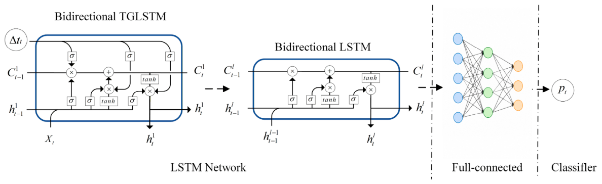
As shown in Figure 4, the first layer is the Time Gate Long Short-Term Memory (TGLSTM). To capture both forward and backward information in the sequence data, we adopted a Bidirectional LSTM instead of a standard LSTM.

A change point identified within three subsequent samples after its occurrence is considered successfully detected. These subsequent observations provide additional temporal information for change point identification. By utilizing both preceding and subsequently available observations, Bidirectional LSTM can achieve better detection performance than conventional LSTM.

The classification section of the network comprises a fully connected layer and a softmax classifier. Specifically, the fully connected layer performs a linear combination and dimensionality reduction on high-level features, while the softmax classifier is responsible for outputting the final class labels.

3.3.2. Bayesian Estimator of Abrupt Change, Seasonality and Trend (BEAST)

BEAST is an algorithm designed for deriving nonlinear ecosystem dynamics across multiple timescales. As an ensemble algorithm, BEAST quantifies the relative usefulness of individual decomposition models, leveraging all the models via Bayesian model averaging. The combination of many models enables BEAST to alleviate model misspecification, address algorithmic uncertainty, and reduce overfitting. BEAST is generically applicable to time series data of all kinds [30].

In BEAST, a time series is composed of three components—seasonality, trend, and abrupt changes plus noise. It abandons the single-best-model paradigm and applies the Bayesian ensemble modeling technique to combine numerous competing models and generate a rich set of information unobtainable from non-Bayesian algorithms. BEAST can quantify various sources of uncertainty, detect abrupt changes of any magnitude and uncover complex nonlinear dynamics from time series data.

Diverging from the conventional ‘single-best-model’ paradigm, this approach employs Bayesian ensemble modeling to infer results by integrating the probabilistic outcomes of numerous competing models, rather than seeking a unique optimal solution. The method has three distinct advantages: the ability to quantify multi-source uncertainties (including model uncertainty), the precise detection of abrupt changes of any magnitude and the effective characterization of complex nonlinear dynamics within the data [30].

4. Results

4.1. Data Simulation

To address the lack of ground truth in interferometric synthetic aperture radar (InSAR) time series, we developed an automated simulation pipeline to generate training and evaluation data. We first generated a large number of baseline deformation sequences. The parameter settings for the simulation are detailed in

Table 1. Initial deformation simulation parameters.

Simulation Parameters	Value
Maximum initial velocity (mm/d)	0.05
Maximum initial acceleration (mm/d2)	0.03
Length of sequences	10–30
Time interval (days)	1
Sampling interval (days)	6

.

The simulation parameters were selected based on the deformation characteristics reported in previous studies. Existing studies have shown that urban subsidence and mining-induced deformation can exhibit significant variations in deformation velocity, acceleration and displacement magnitude [31,32,33,34]. Therefore, the parameter ranges adopted in this study were designed to represent typical nonlinear deformation patterns while providing sufficient diversity for model training and evaluation.

The NRT algorithm based on SE enhances computational efficiency through data grouping. Therefore, the minimum and maximum group sizes were set to 10 and 30 SLC images, respectively. The minimum group size was set to 10 SLC images to ensure sufficient temporal observations for reliable deformation estimation, while the maximum group size was set to 30 SLC images to limit the rapid increase in interferometric combinations and computational burden. These thresholds were therefore adopted as practical bounds to balance deformation estimation reliability and computational efficiency. Therefore, the sequence length was restricted to 10–30 observations.

The simulation time step was set to 1 day, while cumulative deformation was sampled at 6-day intervals, which is comparable to that of the Sentinel-1A and Sentinel-1B satellites.

$$T\left(l\right)=t\left(6l\right),l=1,2\dots L$$

(11)

$T(l)$ denotes the sampled time series, $t\left(l\right)$ denotes the simulated time series, $L$ denotes the length of the sampled time series, and $l$ denotes sampling index.

For a sampled sequence, we first use a probability $P_{tc}$ to determine whether the generated sequence includes acceleration and velocity changes. After that, we use a probability $P_{sc}$ to decide whether to add step changes to the sampled sequence; otherwise, the original sampled sequence is retained. For sequences with trend changes and step changes, based on the type of change point, a random step size $S$ from a probability distribution $P_{step}$ or a velocity $v$ from a probability distribution $P_{vel}$ is added to the sampled time series.

To better represent the complex noise characteristics of real InSAR observations, a semi-synthetic noise model based on Sentinel-1 data was introduced. Stable, high-coherence pixels without significant deformation were selected, and their long-term deformation trends were removed to obtain residual time series, which were regarded as empirical InSAR noise. The residual sequences were centered and retained in their original temporal order to preserve temporally correlated errors associated with atmospheric disturbances, decorrelation and processing residuals. The extracted residual sequences were then scaled according to prescribed signal-to-noise ratio (SNR) levels and superimposed on the simulated deformation signals to generate semi-synthetic observations.

$$SNR=10{\log }_{10}\left({Power}_s/{Power}_n\right)$$

(12)

$SNR$ stands for signal-to-noise ratio, ${Power}_s$ stands for signal power, and ${Power}_n$ for noise power.

Compared with Gaussian white-noise simulations, this strategy provides a more realistic representation of practical InSAR noise conditions and enables a more reliable evaluation of the robustness of the proposed method.

Finally, the simulated time series were generated at a temporal resolution of 1 day and sampled at 6-day intervals. During the construction process, the simulation accounted for missing observations, trend variations and step changes. The specific simulation parameters have been detailed in the

Table 2. Parameters for change-point simulation.

Simulation Parameters	Value
Maximum change velocity (mm/d)	0.2
Minimum change velocity (mm/d)	0.05
Maximum change in acceleration (mm/d2)	0.005
Minimum change in acceleration (mm/d2)	0.002
Maximum step deformation (mm)	20
Minimum step deformation (mm)	10
Size of the training dataset	90,000
Size of the validation dataset	10,000
Maximum SNR (dB)	5
Minimum SNR (dB)	2

.

4.2. Network Architecture Selection

To select the most suitable neural network, LSTM, Bidirectional LSTM and Transformer were compared. The models were trained on the training set and evaluated for performance using the validation set.

LSTM and Bidirectional LSTM share similar architectures—which have already been described in the Section 3. Here, we focus on introducing the Transformer-based classification network.

For the Transformer architecture, the decoding module is primarily used for generating target sequences. However, for time series classification tasks, the objective is to classify the entire deformation sequence rather than generate a target sequence. Therefore, a decoder is not required. The output of the Transformer encoder is passed through a fully connected layer and a softmax classification head to produce the final class probabilities.

The performance of the three network architectures is summarized in

Table 3. Performance comparison of different network architectures.

Method	Accuracy	Precision	Recall	F1
LSTM	83.30%	95.00%	70.28%	80.79%
Bidirectional LSTM	88.43%	90.76%	86.04%	88.34%
Transformer	80.20%	84.84%	71.84%	77.80%

. Considering that a short detection delay does not significantly affect the subsequent deformation estimation in the proposed sequential processing framework, a tolerance window is allowed for change point detection. Specifically, a predicted change point is regarded as a True Positive (TP) if it is identified within three subsequent observations after the actual change point occurs.

Bidirectional LSTM outperforms LSTM in time series classification tasks, primarily due to its ability to use global contextual information. Global information is crucial when classifying entire sequences or specific segments. For instance, an isolated waveform peak might be merely noise; however, if it is accompanied by an overall uplift in the surrounding context, it is more likely to be a step deformation signal. By referencing both past and future sequences during anomaly detection, Bidirectional LSTM’s global view enables the model to detect deformation change points with greater precision and robustness.

The lower performance of the Transformer may be attributed to the characteristics of the present task. The deformation sequences are relatively short, ranging from 10 to 30 time steps, with an average length of approximately 20, which limits the benefit of the Transformer in modeling long-range dependencies. In addition, the Transformer relies more heavily on data-driven learning of temporal relationships. With a limited amount of training data, it may therefore be more difficult to learn stable and generalizable attention patterns. Although increasing the training data improved the performance of the Transformer in our experiments, it still did not outperform Bidirectional LSTM, suggesting that the sequential inductive bias of Bidirectional LSTM may be better suited to the short-term and locally varying temporal characteristics of deformation change point detection.

Because Bidirectional LSTM outperformed both LSTM and Transformer across the evaluation metrics, it was selected as the core network in this study.

4.3. Training Details

To determine the optimal parameters for the Bidirectional LSTM network, we conducted an ablation study focusing on the number of Bidirectional LSTM layers and the hidden-state size.

As shown in

Table 4. Performance of Bidirectional LSTM with different numbers of recurrent layers and hidden-state sizes.

Recurrent Layers	Hidden State Size	F1
2	32	0.726
2	64	0.876
2	128	0.883
2	256	0.879
4	32	0.742
4	64	0.904
4	128	0.935
4	256	0.915
8	32	0.514
8	64	0.510
8	128	0.523
8	256	0.507

, a two-layer Bidirectional LSTM lacks sufficient complexity to address this problem, whereas an eight-layer Bidirectional LSTM suffers from overfitting, resulting in a significant performance drop on the test set. Therefore, we selected the four-layer configuration. The hidden state size was set to 128, which achieved the best F1-score.

The training parameters of the Bidirectional LSTM network are summarized in

Table 5. Training hyperparameters of the Bidirectional LSTM network.

Training Parameters	Setting
Recurrent Layers	4
Hidden state size	128
Optimizer	Adam
Initial learning rate	0.002
Maximum epochs	100
Mini-batch size	64
Shuffle	Every epoch
Gradient threshold	1

.

4.4. Ablation Study of the LSTM–BEAST Two-Stage Framework

To evaluate the necessity of the Bidirectional LSTM pre-screening module, an ablation experiment was conducted by comparing Bidirectional LSTM with BEAST alone to determine whether a deformation sequence contains a change point. For BEAST, the seasonal component was disabled, the allowable number of trend change points was set to 0–1 and the trend polynomial order was limited to 0–2. The same parameter settings were used for all test samples.

As shown in

Table 6. Performance comparison between Bidirectional LSTM and BEAST under different SNR conditions.

Noise Condition	Method	Accuracy	Precision	Recall	F1
SNR = 5 dB	Bidirectional LSTM	96.20%	98.42%	94.33%	96.33%
SNR = 5 dB	BEAST	61.30%	100.00%	26.84%	42.32%
SNR = 2 dB	Bidirectional LSTM	80.20%	84.84%	71.84%	77.80%
SNR = 2 dB	BEAST	63.90%	92.96%	27.33%	42.24%

, Under SNR = 5 dB, Bidirectional LSTM achieved an accuracy of 96.20%, a recall of 94.33% and an F1-score of 96.33%, whereas BEAST achieved 61.30%, 26.84% and 42.32%, respectively. Under SNR = 2 dB, Bidirectional LSTM achieved an accuracy of 80.20%, a recall of 71.84% and an F1-score of 77.80%, while BEAST achieved 63.90%, 27.33% and 42.24%, respectively.

Although BEAST achieved high precision, its relatively low recall indicates that many sequences containing true change points were missed. These results demonstrate that Bidirectional LSTM is more suitable for change-existence screening in short deformation sequences, while BEAST is subsequently used for precise change point localization. Therefore, the two modules play complementary roles in the proposed two-stage framework.

4.5. Effectiveness Analysis of TGLSTM Under Missing-Data Conditions

To evaluate the contribution of sampling-interval information to TGLSTM under missing-data conditions, 10% of the sampling points were randomly removed from the original sequences. Two models with the same architecture were then compared, differing only in the temporal information provided to the TGLSTM layer. One model used the actual sampling intervals after data removal, whereas the other used artificially generated uniform intervals. As shown in

Table 7. Performance comparison using actual and uniform sampling intervals under missing-data conditions.

Method	Accuracy	Precision	Recall	F1
Uniform sampling intervals	90.94%	92.65%	88.94%	90.76%
Actual sampling intervals	91.47%	93.17%	91.33%	92.25%

, Using the actual sampling intervals improved the F1-score by approximately 1.5%, indicating that TGLSTM can effectively utilize sampling-interval information to account for irregular sampling caused by missing observations and thereby improve change point detection performance.

4.6. Comparison Methods

In this study, we evaluate the efficacy of the proposed method by conducting a comparative analysis against several existing techniques, including the Cumulative Sum (CUSUM) and Bayesian Online Change Point Detection (BOCPD) algorithms.

The cumulative deformation sequences were standardized before being input into the CUSUM detector. A two-sided CUSUM was employed with a reference value $k=0.5$ and a decision threshold $h=5$. For BOCPD, a constant hazard function was adopted. Since the simulated sequences contained 20 observations and approximately 50% of the sequences included a change point, $\lambda =30$ was used in the experiments.

A detected change point was considered correct if its estimated location fell within three samples before or after the ground-truth change point. Otherwise, the detection was regarded as incorrect. The outcomes of this experiment are presented in

Table 8. Performance comparison of different change-point detection methods.

Method	Accuracy	Precision	Recall	F1
CUSUM	69.71%	70.38%	68.06%	69.20%
BOCPD	83.26%	78.89%	90.82%	84.44%
Proposed Method	91.45%	93.64%	88.94%	91.23%

.

The proposed method achieved the highest F1-score and precision among the three methods.

4.7. Comparison Using Simulated Cumulative Deformation Sequences

The proposed Grouping Strategy is compared against the StBAS employed by SE. We generated 100,000 deformation sequences with lengths varying from 300 to 400 days, sampled at a 6-day interval. Following the method proposed in Section 4.1, we introduced step changes, abrupt variations in velocity and acceleration and random noise. Relevant parameters are referenced in Table 2. The final dataset comprises time series of lengths varying between 50 and 67, including time series without change points, time series with step change points and time series with velocity and acceleration change points.

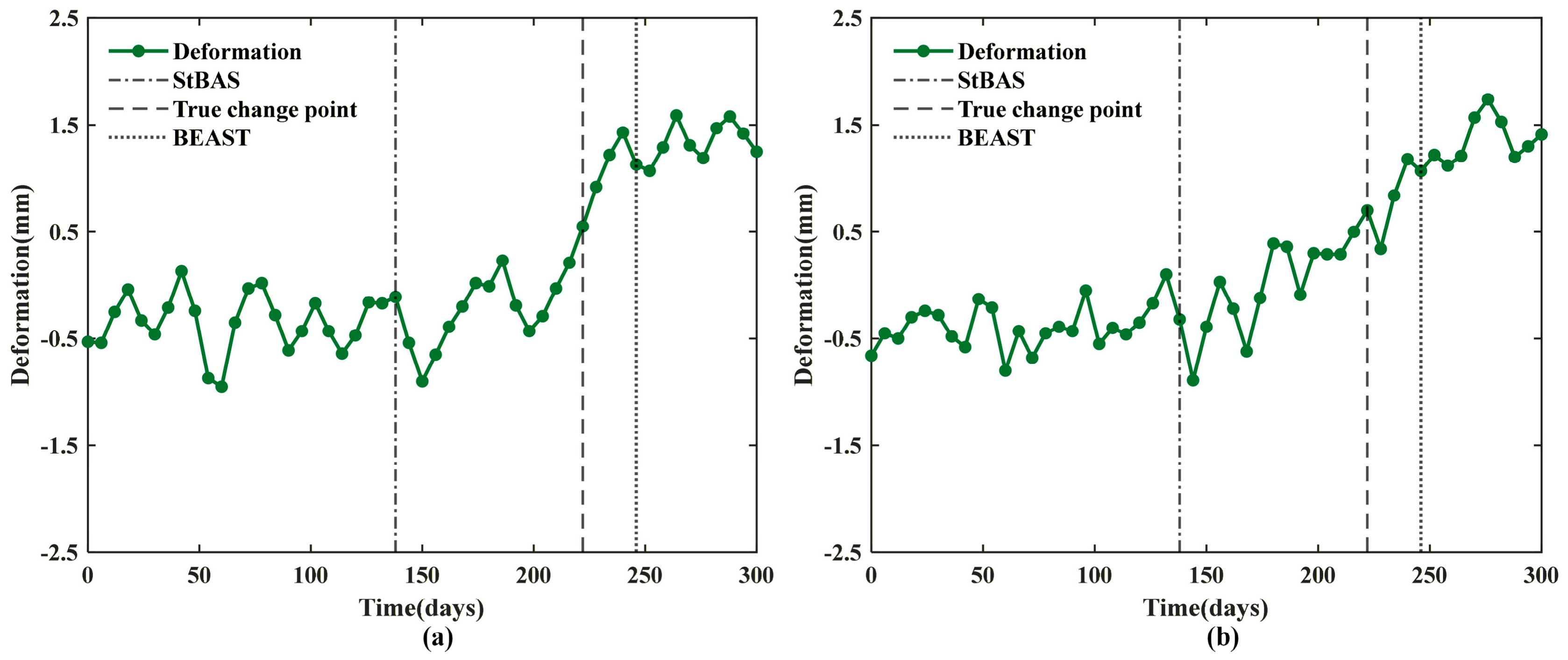
All time series were analyzed using StBAS and the Change-Point-Based Deformation Grouping Strategy; the results are illustrated in Figure 5. The true deformation change points were also employed as a control baseline to validate the experimental results.

Figure 5a shows the simulated time series with a step change point; Figure 5b shows the simulated time series with acceleration and velocity change point. It is worth noting that BEAST is capable of detecting both step changes and velocity/acceleration changes within 30 days (i.e., 5 sampling points).

4.8. Robustness Analysis

To evaluate the robustness of the Bidirectional LSTM model for change point detection, we conducted a systematic simulation study. The study primarily investigated three key parameters: the relationship between the signal-to-noise ratio (SNR) and the magnitude of velocity changes, the relationship between SNR and acceleration changes, and the relationship between SNR and the magnitude of step changes. For each parameter combination, 10,000 time series were generated for model training and testing. The specific parameters of the simulated time series are detailed in Section 4.1, and the results are evaluated using the F1-score.

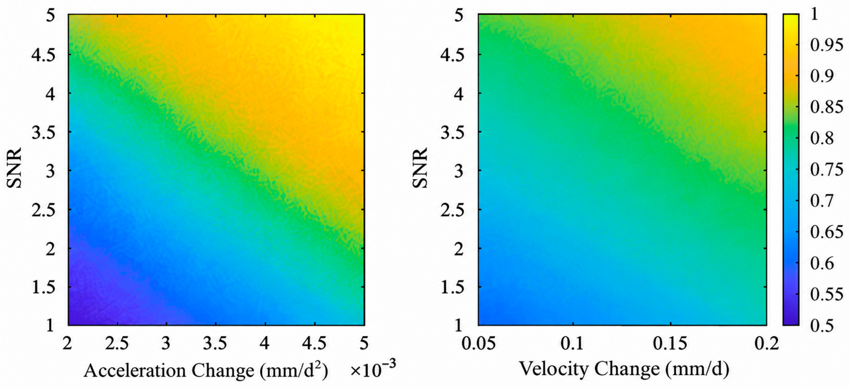
As shown in Figure 6, the left figure shows the F1-score of the proposed model under different SNR levels and magnitudes of acceleration changes; the right figure shows the F1-score of the proposed model under different Signal-to-Noise Ratios (SNR) and magnitudes of velocity changes. It demonstrates that the model is sensitive to changes in velocity and acceleration. However, when the acceleration changes are small, the F1-score is suboptimal. Specifically, under conditions of both low Signal-to-Noise Ratio (SNR) and low acceleration changes, the algorithm′s F1-score can drop to as low as 0.6. This limitation is likely due to the short length of the time series used in the experiments. For velocity changes, model performance is more stable, with the F1-score generally remaining around 0.8.

4.9. Real Data

4.9.1. Deformation with Changes in Velocity and Acceleration

Ground deformation is generally influenced by multiple natural and anthropogenic factors, and its temporal evolution often manifests as changes in deformation velocity and acceleration. Such changes are particularly common in long-term deformation monitoring, where variations in groundwater conditions, precipitation, surface loading and human activities can alter the deformation rate and even reverse the deformation trend.

Beijing provides a representative example of this type of deformation. Long-term groundwater overexploitation has resulted in significant land subsidence in Beijing. However, following the implementation of the South-to-North Water Diversion Project and groundwater conservation measures, groundwater conditions have gradually improved, leading to substantial changes in the original deformation behavior [35]. In some areas, the subsidence rate has gradually decreased, and a transition from subsidence to surface uplift has been observed. Such a transition is reflected in the deformation time series as pronounced changes in deformation velocity and acceleration.

The long-term deformation dataset was acquired by Sentinel-1 in Interferometric Wide Swath (IW) mode along an ascending orbit and comprises 200 SLC images acquired between 22 January 2019 and 23 September 2025. The study area is in Shunyi District, Beijing, and the groundwater-level sampling site used for comparison is located in Wali Village, Shunyi District, Beijing. It should be noted that the same pre-trained model was directly applied to all real-world datasets without any additional site-specific retraining, fine-tuning, or parameter adjustment.

We first used all available SLC images to obtain the complete cumulative deformation time series. Subsequently, following the method described in Section 3, the data were processed sequentially in groups to perform near-real-time deformation change point detection.

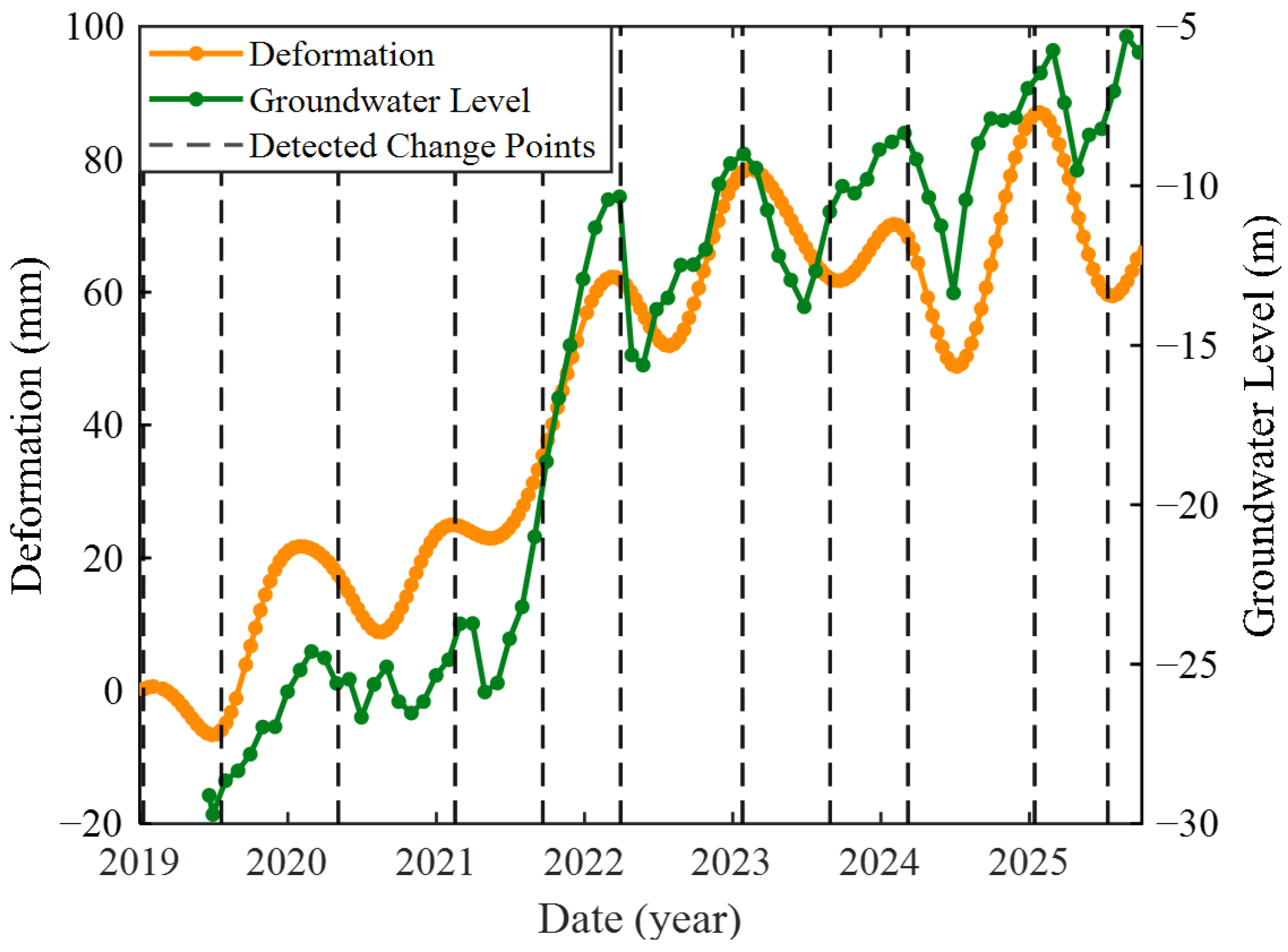
To further evaluate the physical relevance of the detected change points, the Beijing deformation time series was compared with independent groundwater-level observations. As shown in Figure 7, several detected change points occur close to groundwater-level variations and corresponding changes in the deformation trend. The temporal consistency between groundwater fluctuations and deformation transitions indicates that the identified change points are associated with physically meaningful changes in the deformation process. This comparison provides independent external support for the reliability of the detected deformation change points.

4.9.2. Step-like Deformation

Step-like deformation is characterized by an abrupt displacement over a short period, resulting in a clear transition between two deformation states.

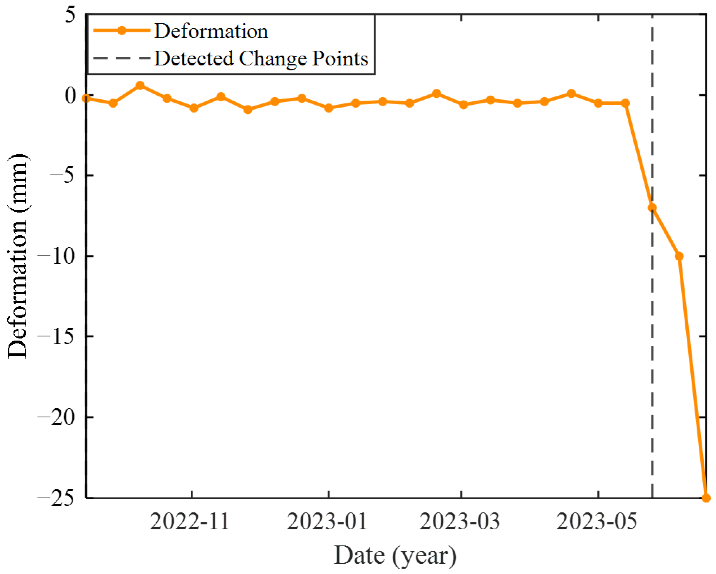
On 31 May 2023, a sudden ground subsidence event occurred in Balitai Town, Jinnan District, Tianjin City. The event was associated with improper geothermal well drilling, which intersected a large underground karst cavity and caused wellbore leakage. The rapid migration of drilling fluid into the cavity and the resulting pressure imbalance induced the collapse and downward movement of the overlying sandy soil, ultimately triggering rapid surface subsidence [28]. The deformation dataset used for analysis consisted of 24 Sentinel-1 C-band SAR images acquired between 15 September 2022 and 18 June 2023. InSAR observations indicate that the area remained relatively stable before 23 May 2023, followed by rapid subsidence exceeding 10 mm within a short period.

As shown in Figure 8, the deformation time series remained relatively stable from September 2022 to May 2023, with only small fluctuations around the initial deformation state. A pronounced downward displacement then occurred in late May 2023, marking a clear transition from the stable stage to rapid subsidence. The detected change point is located close to the onset of the abrupt deformation and is temporally consistent with the reported subsidence event on 31 May 2023. This result indicates that the proposed method can effectively identify step-like deformation changes characterized by a sudden transition between deformation states.

5. Discussion

The robustness analysis indicates that model performance degrades primarily under severe noise conditions, suggesting that future improvements should focus on low-SNR cases. First, the training dataset could be enriched with a larger proportion of low-SNR samples, particularly those close to the current detection limit, to improve the sensitivity of the model to subtle nonlinear deformation patterns. In addition, longer historical information could be incorporated into the change point screening process without changing the current group-size constraint. Specifically, when a low-SNR situation is detected in the preceding stage, the subsequent observations could be jointly analyzed with part of the previously accumulated deformation sequence. This additional temporal context may help the model capture gradual and persistent curvature variations that are difficult to distinguish from noise within a short sequence of 10–30 observations. In this way, the grouping size can remain unchanged for deformation estimation, while the change point detection module can exploit a longer effective temporal context to improve the identification of previously missed weak deformation changes.

Periodic deformation should also be considered when applying the proposed method to short deformation sequences. Seasonal deformation may be caused by groundwater fluctuations, thermal expansion and other environmental factors. However, because each group in the proposed framework contains only 10–30 observations, an individual group may not cover sufficient cycles to reliably estimate periodic components. A partial periodic signal may therefore resemble a nonlinear trend or an apparent change point, potentially affecting change point detection. This study focuses primarily on step-like deformation and changes in deformation velocity and acceleration. Incorporating longer-term historical information or explicit seasonal modeling to distinguish periodic deformation from genuine deformation transitions will be investigated in future work.

6. Conclusions

To reduce deformation estimation errors caused by nonlinear temporal behavior in long-term monitoring, we propose a Change-Point-Based Deformation Grouping Strategy (CPDGS) for NRT InSAR. The proposed framework integrates a Bidirectional LSTM network with BEAST. The Bidirectional LSTM first determines whether a deformation time series contains a change point, and BEAST subsequently localizes the detected change point.

(1)

The integrated framework combines a Bidirectional LSTM network and the BEAST algorithm: the Bidirectional LSTM module first screens the deformation sequence for the presence of change points, whereas BEAST subsequently determines their locations. The utilization of the network addresses the issue of BEAST inaccurately estimating the number of change points. Conversely, BEAST mitigates the problem of the LSTM failing to precisely detect change point locations in noisy environments.

(2)

Considering the scarcity of reliable field-measured ground truth data, simulated deformation time series are generated for network training, thereby enabling quantitative evaluation and systematic validation of the model’s change point detection performance.

(3)

The experimental results demonstrate the effectiveness of the proposed framework. In the comparative change point detection experiment, the proposed method achieved an F1-score of 91.23%, outperforming CUSUM (69.20%) and BOCPD (84.44%). The applicability of the proposed method was further examined using real Sentinel-1 deformation time series. In the Beijing case, several detected deformation change points were temporally consistent with pronounced groundwater-level variations. In the Tianjin case, the detected change point closely coincided with the documented ground-subsidence event on 31 May 2023. These results demonstrate the potential of CPDGS for long-term sequential deformation monitoring.

In summary, CPDGS achieves a favorable balance between computational efficiency and deformation retrieval accuracy by restricting the maximum number of images in each group and accurately identifying abrupt deformation points. The relevant research results can provide a reference for NRT InSAR data grouping.

Future work will focus on improving the sensitivity of the model to weak acceleration changes by incorporating longer temporal context, more diverse training samples, and more robust temporal feature extraction. In addition, validation using more independent GNSS or leveling observations will be explored to further improve the generalization and practical applicability of the proposed framework.

References

- Herrera-García, G.; Ezquerro, P.; Tomás, R.; Béjar-Pizarro, M.; López-Vinielles, J.; Rossi, M.; Mateos, R.M.; Carreón-Freyre, D.; Lambert, J.; Teatini, P.; et al. Mapping the global threat of land subsidence. Science 2021, 371, 34–36. [Google Scholar] [CrossRef] [Scilit] [PubMed]
- Ao, Z.; Hu, X.; Tao, S.; Hu, X.; Wang, G.; Li, M.; Wang, F.; Hu, L.; Liang, X.; Xiao, J.; et al. A national-scale assessment of land subsidence in China’s major cities. Science 2024, 384, 301–306. [Google Scholar] [CrossRef] [Scilit] [PubMed]
- Zhang, L.; Chen, J.; Chen, L.; Luo, Y.; Liu, W. Deformation grading and prediction of heterogeneous layered soft rock tunnels under high ground-stress: A case study. Tunn. Undergr. Space Technol. 2026, 167, 107071. [Google Scholar] [CrossRef] [Scilit]
- Wang, J.; Hu, S.; Wang, T.; Liang, H.; Yang, Z. GNSS Horizontal Motion Field in the Beijing Plain in View of The Variation Characteristics of The 3D Deformation Field. Remote Sens. 2023, 15, 787. [Google Scholar] [CrossRef] [Scilit]
- Lee, J.-S.; Jeong, S.H.; Park, G.; Kim, Y.; Tutumluer, E.; Kim, S.Y. Geotechnical Application of Unmanned Aerial Vehicle (UAV) for Estimation of Ground Settlement after Filling and Compaction. Transp. Geotech. 2025, 51, 101517. [Google Scholar] [CrossRef] [Scilit]
- Ge, Z.; Wu, W.; Hu, J.; Muhetaer, N.; Zhu, P.; Guo, J.; Li, Z.; Zhang, G.; Bai, Y.; Ren, W. Evaluating the Interferometric Performance of China’s Dual-Star SAR Satellite Constellation in Large Deformation Scenarios: A Case Study in the Jinchuan Mining Area, Gansu. Remote Sens. 2025, 17, 2451. [Google Scholar] [CrossRef] [Scilit]
- Ma, P.; Chen, L.; Yu, C.; Zhu, Q.; Ding, Y.; Wu, Z.; Li, H.; Tian, C.; Fan, X. Dynamic landslide susceptibility mapping over last three decades to uncover variations in landslide causation in subtropical urban mountainous areas. Remote Sens. Environ. 2025, 326, 114800. [Google Scholar] [CrossRef] [Scilit]
- Mohammadnia, M.; Yip, M.W.; Webb, A.A.G.; González, P.J. Spontaneous Transient Summit Uplift at Taftan Volcano (Makran Subduction Arc) Imaged Using an InSAR Common-Mode Filtering Method. Geophys. Res. Lett. 2025, 52, e2025GL114853. [Google Scholar] [CrossRef] [Scilit]
- Zhao, Q.; Zhang, Y.; Pepe, A.; Mastro, P.; Zheng, T.; Yang, T. Coupled ground subsidence and rapid urbanization of the Red River delta region and the city of Hanoi, Vietnam, revealed through a Multi-Track InSAR analysis. Int. J. Appl. Earth Obs. Geoinf. 2025, 144, 104886. [Google Scholar] [CrossRef] [Scilit]
- Wang, L.; Zhao, L.; Liu, S.; Zhou, H.; Hu, G.; Zou, D.; Du, E.; Liu, G.; Xiao, Y.; Chen, Y.; et al. Evaluation of stability and cooling engineering effectiveness of the Qinghai-Tibet transportation routes: A first comprehensive assessment using space geodetic observations. Eng. Geol. 2026, 361, 108502. [Google Scholar] [CrossRef] [Scilit]
- Ma, P.; Wu, Z.; Zhang, Z.; Au, F.T.K. SAR-Transformer-based decomposition and geophysical interpretation of InSAR time-series deformations for the Hong Kong-Zhuhai-Macao Bridge. Remote Sens. Environ. 2024, 302, 113962. [Google Scholar] [CrossRef] [Scilit]
- Karamvasis, K.; Karathanassi, V. Performance Analysis of Open Source Time Series InSAR Methods for Deformation Monitoring over a Broader Mining Region. Remote Sens. 2020, 12, 1380. [Google Scholar] [CrossRef] [Scilit]
- Nurzaman, F.; Izumi, Y.; Sato, M.; Urano, K.; Kawamura, S.; Tetuko Sri Sumantyo, J.; Ota, K.; Dong, M.; Wijaya, D.D. A Robust APS Trend Estimation Technique for Ground-Based InSAR Measurements of Urban Landslide. IEEE Geosci. Remote Sens. Lett. 2024, 21, 4016905. [Google Scholar] [CrossRef] [Scilit]
- Cian, F.; Blasco, J.M.D.; Carrera, L. Sentinel-1 for Monitoring Land Subsidence of Coastal Cities in Africa Using PSInSAR: A Methodology Based on the Integration of SNAP and StaMPS. Geosciences 2019, 9, 124. [Google Scholar] [CrossRef] [Scilit]
- Hussain, S.; Pan, B.; Hussain, W.; Sajjad, M.M.; Ali, M.; Afzal, Z.; Abdullah-Al-Wadud, M.; Tariq, A. Integrated PSInSAR and SBAS-InSAR analysis for landslide detection and monitoring. Phys. Chem. Earth Parts A/B/C 2025, 139, 103956. [Google Scholar] [CrossRef] [Scilit]
- Li, S.; Xu, W.; Li, Z. Review of the SBAS InSAR Time-series algorithms, applications, and challenges. Geod. Geodyn. 2022, 13, 114–126. [Google Scholar] [CrossRef] [Scilit]
- Kuzuoka, S.; Ferretti, A.; Novaliaro, F. A new algorithm to monitor surface deformation: SQUEESAR. In Global Meeting Abstracts, Proceedings of the 11th SEGJ International Symposium, Yokohama, Japan, 18-21 November 2013; Society of Exploration Geophysicists: Houston, TX, USA, 2013; pp. 9–10. [Google Scholar]
- De, L. A First Quantitative Assessment of the P-SBAS Approach Capability to Retrieve SAOCOM-1 DInSAR Deformation Time Series over the Italian Territory. In Proceedings of the EUSAR 15th European Conference on Synthetic Aperture Radar, Munich, Germany, 23–26 April 2024; pp. 879–883. [Google Scholar]
- Ma, Z.; Liu, J.; Aoki, Y.; Wei, S.; Liu, X.; Cui, Y.; Hu, J.; Zhou, C.; Qin, S.; Huang, T.; et al. Towards big SAR data era: An efficient Sentinel-1 Near-Real-Time InSAR processing workflow with an emphasis on co-registration and phase unwrapping. ISPRS J. Photogramm. Remote Sens. 2022, 188, 286–300. [Google Scholar] [CrossRef] [Scilit]
- Ansari, H.; De Zan, F.; Bamler, R. Sequential Estimator: Toward Efficient InSAR Time Series Analysis. IEEE Trans. Geosci. Remote Sens. 2017, 55, 5637–5652. [Google Scholar] [CrossRef] [Scilit]
- Wang, B.; Zhao, C.; Zhang, Q.; Lu, Z.; Li, Z.; Liu, Y. Sequential Estimation of Dynamic Deformation Parameters for SBAS-InSAR. IEEE Geosci. Remote Sens. Lett. 2020, 17, 1017–1021. [Google Scholar] [CrossRef] [Scilit]
- Ao, M.; Wei, L.; Liao, M.; Zhang, L.; Dong, J.; Liu, S. Incremental multi temporal InSAR analysis via recursive sequential estimator for long-term landslide deformation monitoring. ISPRS J. Photogramm. Remote Sens. 2024, 215, 313–330. [Google Scholar] [CrossRef] [Scilit]
- Costa, G.; Monti Guarnieri, A.V.; Manzoni, M.; Parizzi, A. BUD: Band-limited uncalibrated detector of environmental changes for InSAR monitoring framework. ISPRS J. Photogramm. Remote Sens. 2025, 230, 55–72. [Google Scholar] [CrossRef] [Scilit]
- An, L.; Yu, W.; Wang, J.; Li, H.; Wang, H.; Wu, Y. A Novel Statistically Homogeneous Pixels Updating Algorithm for Long-Term Near-Real-Time Deformation Monitoring. IEEE Geosci. Remote Sens. Lett. 2024, 21, 4018805. [Google Scholar] [CrossRef] [Scilit]
- Vu, P.V.H.; Brigui, F.; Breloy, A.; Yan, Y.; Ginolhac, G. A New Phase Linking Algorithm for Multi-Temporal InSAR Based on the Maximum Likelihood Estimator. In Proceedings of the IGARSS Kuala Lumpur, Kuala Lumpur, Malaysia, 17–22 July 2022; pp. 76–79. [Google Scholar]
- Vu, P.V.H.; Breloy, A.; Brigui, F.; Yan, Y.; Ginolhac, G. Robust Phase Linking in InSAR. IEEE Trans. Geosci. Remote Sens. 2023, 61, 5211111. [Google Scholar] [CrossRef] [Scilit]
- Eppler, J.; Rabus, B.T. Adapting InSAR Phase Linking for Seasonally Snow-Covered Terrain. IEEE Trans. Geosci. Remote Sens. 2022, 60, 4305313. [Google Scholar] [CrossRef] [Scilit]
- Jiang, H.; Balz, T.; Li, J.; Mishra, V. Preliminary Investigation of Sudden Ground Subsidence and Building Tilt in Balitai Town, Tianjin City, on 31 May 2023. Remote Sens. 2023, 15, 4891. [Google Scholar] [CrossRef] [Scilit]
- Shimosato, K.; Ukita, N. Multi-Modal Data Fusion for Land-Subsidence Image Improvement in PSInSAR Analysis. IEEE Access 2021, 9, 141970–141980. [Google Scholar] [CrossRef] [Scilit]
- Zhao, K.; Wulder, M.A.; Hu, T.; Bright, R.; Wu, Q.; Qin, H.; Li, Y.; Toman, E.; Mallick, B.; Zhang, X.; et al. Detecting change-point, trend, and seasonality in satellite time series data to track abrupt changes and nonlinear dynamics: A Bayesian ensemble algorithm. Remote Sens. Environ. 2019, 232, 111181. [Google Scholar] [CrossRef] [Scilit]
- Siles, G.; Alcérreca-Huerta, J.; López-Quiroz, P.; Niemeier, W. Long Term Subsidence Analysis and Soil Fracturing Zonation Based on InSAR Time Series Modelling in Northern Zona Metropolitana del Valle de Mexico. Remote Sens. 2015, 7, 6908–6931. [Google Scholar] [CrossRef] [Scilit]
- Zhang, Q.; Guo, Z.; Wang, M.; Mei, J.; Liu, L.; Ashraf, T.; Wang, X. InSAR-Based Multi-Source Monitoring and Modeling of Multi-Seam Mining-Induced Deformation and Hazard Chain Evolution in the Loess Gully Region. Remote Sens. 2025, 17, 3993. [Google Scholar] [CrossRef] [Scilit]
- Bao, L.; Zhang, G.; Hu, X.; Wu, S.; Liu, X. Stage Division of Landslide Deformation and Prediction of Critical Sliding Based on Inverse Logistic Function. Energies 2021, 14, 1091. [Google Scholar] [CrossRef] [Scilit]
- Zhou, B.; Li, S.; Kang, J.; Zhang, L.; Zhang, J.; Li, M. A probability integral method modified model for accurately characterizing subsidence at the boundary of a mining area. Sci. Rep. 2025, 15, 21014. [Google Scholar] [CrossRef] [Scilit] [PubMed]
- Fu, Y.; Wang, J.; Zhang, Y.; Yang, H.; Li, L.; Ren, Z. Spatiotemporal evolution characteristics of ground deformation in the Beijing Plain from 1992 to 2023 derived from a novel multi-sensor InSAR fusion method. Remote Sens. Environ. 2025, 319, 114635. [Google Scholar] [CrossRef] [Scilit]
Figure 1.
Flowchart of the Sequential Estimator (SE) and Recursive Sequential Estimator with Flexible Batches (RSEFB), the differences between the two methods are highlighted in red text for clarity.
Figure 2.
Flowchart of the proposed Change-Point-Based Deformation Grouping Strategy for initial processing.
Figure 3.
Flowchart of the proposed sequential processing framework.
Figure 4.
Architecture of the proposed Bidirectional Time Gate Long Short-Term Memory (TGLSTM)–Long Short-Term Memory (LSTM) classification network.
Figure 5.
Comparison of deformation grouping results for different types of change points. (a) Step-like deformation; (b) deformation with velocity and acceleration changes.
Figure 6.
F1-score of the proposed model under different Signal-to-Noise Ratios (SNR) and magnitudes of velocity and acceleration changes.
Figure 7.
Comparison of ground deformation, groundwater-level variations and detected change points in Shunyi District, Beijing.
Figure 8.
Ground deformation time series and detected change point associated with the sudden subsidence event in Balitai Town, Tianjin.