Article

Comparing Modelled and Remotely Sensed Soil Moisture Products Using In Situ Observations in Liguria, Italy: Evaluation via SWI Filtering and Rescaling Techniques


1
CIMA Research Foundation, 17100 Savona, Italy
2
Climate, Weather, and Hydrology Unit, Regional Agency for Environmental Protection in Liguria (U.O. CMI ARPAL), 16129 Genova, Italy
3
Department of Civil, Chemical and Environmental Engineering (DICCA), University of Genova, 16145 Genova, Italy
*
Author to whom correspondence should be addressed.
Remote Sens. 2026, 18(17), 2903; https://doi.org/10.3390/rs18172903
Submission received: 17 June 2026 / Revised: 14 August 2026 / Accepted: 24 August 2026 / Published: 28 August 2026

Highlights

What are the main findings?
  • Rescaled modelled and satellite-based soil moisture (SM) products were compared against the Operational Ground Measurement Network of the Liguria Region.
  • Five rescaling methodologies were tested and compared to reduce the systematic biases between the SM products and in situ observations.
What are the implications of the main findings?
  • In this case study, the rescaled outputs of the Continuum and HTESSEL models generally outperform the satellite-derived rescaled Soil Water Index.
  • For this application, CDF matching techniques and linear regression efficiently reduce bias between the ground measurements and the SM product.

Abstract

Soil Moisture (SM) represents the temporary storage of water within the shallow layers of the Earth’s upper surface and plays a key role in a wide range of applications, including hydrological processes, numerical weather prediction models and landslide prediction. This study evaluates the comparability of multiple satellite- and model-based SM products against in situ volumetric water content (VWC) measurements collected by a regional monitoring network in Liguria, Italy. The analyzed dataset comprises satellite-based products from the SMAP mission and the ASCAT sensors, as well as modelled Soil Moisture outputs from the HTESSEL land surface model and the Root Zone Soil Moisture (RZ SM) estimates from the continuous, distributed and physically based hydrological model Continuum. Aiming to reduce the systematic differences between the SM products and the ground network measurements, Soil Water Index (SWI) filtering and various rescaling techniques are applied and evaluated. Finally, the agreement between the rescaled SM products and the in situ measurements was assessed using standard performance scores aggregated into a single multi-objective function. Within the specific context of the study area, results suggest that rescaled model-based soil moisture products generally outperform satellite-derived surface soil moisture in reproducing in situ observations. Furthermore, among the tested rescaling techniques, Cumulative Distribution Function (CDF) matching and linear regression provide the best performance in mitigating systematic biases. Additionally, the optimization of the characteristic time length (τ) for satellite-derived SWI significantly enhances the agreement with in situ root-zone dynamics.

1. Introduction

Soil moisture plays a key role in hydrological processes, influencing run-off generation and, consequently, catchment responses [1]. It is a key variable for flood monitoring and prediction [2,3,4], particularly in regions exposed to extreme rainfall events and prone to flash floods.
Global distributed SM products suitable for hydrological applications are commonly derived from satellite-based radar and radiometer observations and hydrological or land surface models. However, these datasets are subjected to inherent uncertainties which require correct interpretations [5,6]. A major constraint on satellite-based products is that Surface Soil Moisture (SSM) retrieval strongly depends on surface condition and vegetation density. Conversely, the accuracy of model-derived outcomes is influenced by the quality and availability of meteorological observations and by the knowledge of soil texture and hydraulic properties [3], as well as the specific model structure, internal process representation, and parameterization schemes. To address these inherent uncertainties, accurate in situ continuous monitoring networks serve as a critical baseline for evaluating and validating large-scale satellite and model-based soil moisture products across varied environmental conditions [7,8,9], often relying on International Soil Moisture Network (ISMN). In contrast, regional operational networks, such as the OMIRL observatory in Liguria (https://omirl.regione.liguria.it/ (accessed on 15 April 2026)), are designed for a different primary purpose: real-time hydrological monitoring and forecasting at the event scale to directly support early warning procedures.
Given the operational importance of these local observatories, the main objective of this study is to investigate the agreement between various rescaled satellite- and model-based SM products and in situ measurements within a Mediterranean environment, focusing specifically on the Liguria region (Italy) by using the VWC ground observations provided by the OMIRL network.
To achieve this objective, a specific set of datasets was selected based on their relevance for operational hydrometeorological applications. The datasets analyzed include distributed satellite-based products—specifically, the Soil Moisture Active Passive (SMAP) SPL2SMP_E product [10,11], and H-SAF ASCAT Surface Soil Moisture dataset [12]—as well as model-based outputs such as the two top-soil moisture layer estimates from the European Centre for Medium-Range Weather Forecasts (ECMWF) through the Hydrology Tiled ECMWF Scheme for Surface Exchanges over Land (HTESSEL) Land Surface Model [13] and the Root Zone Soil Moisture (RZ SM) derived from the distributed physical-based hydrological model Continuum (HMC) [14].
The selection of these datasets was driven by their relevance for operational hydrometeorological applications, while HMC is implemented at quite high resolution on the Liguria Region basins, and it is already used operationally providing a consistent long-term historical soil moisture dataset. Instead, HTESSEL, SMAP, and ASCAT were selected for their relatively low latency between data acquisition and availability, making them suitable for near-real-time applications.
By bringing these specific datasets and local ground observations together, one of the most relevant scientific contributions of this study is the development of an integrated framework to compare different SM products with a common ground-based monitoring network. The analysis considers not only statistical performance, but also spatial resolution, sampling strategy, analysis period, rescaling methods, parameter calibration, and local surface characteristics. This helps to better understand the conditions under which satellite- and model-based soil moisture products can accurately represent local ground observations, particularly in areas characterized by highly complex orography and dense vegetation, such as the Ligurian Region.
Testing soil moisture retrievals in these challenging terrains is essential, as satellite observations often suffer from dense vegetation coverage, radio-frequency interference (RFI), urban or water contamination, and topographic shading [15,16,17], while distributed models could face severe limitations in spatial parameterization and representativeness errors [6,15]. Moreover, although various studies have been conducted to evaluate satellite and modelled soil moisture estimations, no specific studies are available for the study area that consider all the sources of soil moisture analyzed in this work.
Beyond this, an additional contribution of this study is the potential application of the proposed framework in an operational, day-by-day system. Since the analyzed soil moisture products are available with relatively low latency, the comparison with in situ observations could be automatically updated as new data become available. Such an approach would allow the recent behaviour and consistency of the different products to be continuously assessed, providing additional information for operational hydrological monitoring and flood forecasting.
The use of satellite soil moisture observations in near-real-time and operational hydrological applications has already been demonstrated in previous studies, including applications within the European Flood Awareness System [18] while recent developments have further improved the availability of low-latency SMAP products for near-real-time applications [19].
The paper is organized as follows: Section 2.1 provides a brief introduction to the SM variable and its equations. The case study is described in Section 2.2, and the datasets are presented in Section 2.3. The methodology on the bias reduction, filtering and performance evaluation is detailed in Section 2.4. Subsequently, the results and some examples are reported in Section 3 and finally the discussion are provided in Section 4.

2. Materials and Methods

2.1. Definitions

In this study, SM is expressed through two quantities: Volumetric Water Content (VWC) and degree of saturation (S). VWC is the ratio between volume of water (Vw) and the volume of total soil (Vt) including water, air and solid fraction. With all the connected pores filled, VWC reaches its saturation value equal to the soil porosity η . By normalization of the VWC respect to the saturation degree S can be computed ( S = V W C η ). While both VWC and S can be expressed either as percentages or dimensionless fractions [0–1], all values in this study were rescaled and are presented as VWC [ m 3 m 3 ].

2.2. Study Area and Case Study

This study was conducted to support a technical evaluation within the operational hydrological forecasting framework of the Ligurian Hydrometeorological Functional Centre (CFMI-PC) [20]. The Liguria region, where the CFMI-PC operates, is a small Mediterranean region on the northwest of Italy, characterized by an east–west elongated shape. Drainage basins range from 10 to 1000 km2, catchment response times vary between 0.5 and 10 h, making the region prone to flash flood [21]. It shows high soil moisture variability and is historically affected by heavy rainfall events leading to disastrous consequences. Winter seasons are temperate, with snowfall typically occurring a few days per year, mainly in the inland and rarely affecting the coastal region [22]. Altitude ranges from sea level to more than 2000 m a.s.l with the highest peak at Monte Saccarello (2200 m a.s.l.). Based on the 2015–2025 averages (https://ambientepub.regione.liguria.it/SiraQualMeteo/script/PubAccessoDatiMeteo.asp (accessed on 24 July 2026)), the monitored stations reveal annual precipitation ranging from 822.4 mm at the warmest site (Albenga Isolabella, 16.4 °C) to 2241.0 mm, 2097.8 mm, and 2090.4 mm at wetter inland locations (Cuccarello, Amborzasco, and Urbe—Vara Sup.). Data from the other sites (Colle D’Oggia, Loco Carchelli, Mignanego, Ognio, and Valzemola) show precipitation levels between 881.7 mm and 1800.2 mm, and average temperatures ranging from 10.7 °C to 13.9 °C.
As described in the following Section 2.3.1, the Frequency Domain Reflectometer (FDR) sensors are strategically placed to cover different elevation and to span the region from east to west.

2.3. Dataset

The datasets analyzed in this study are summarized in Table 1 and are divided into three main groups.
The first group consists of in situ VWC point measurements (Section 2.3.1), which were used as the reference for the rescaling and performance evaluation procedures.
The second group includes satellite-based surface SSM products, namely the SMAP product (expressed as VWC, detailed in Section 2.3.4) and the ASCAT product (expressed as a degree of saturation, detailed in Section 2.3.5).
Finally, the third group comprises model-based SM estimates, including outputs from the HTESSEL land surface model (Section 2.3.3) and the Continuum hydrological model (Section 2.3.2), both expressed as a degree of saturation.

2.3.1. Ground Measurement Network: VWC Time Series

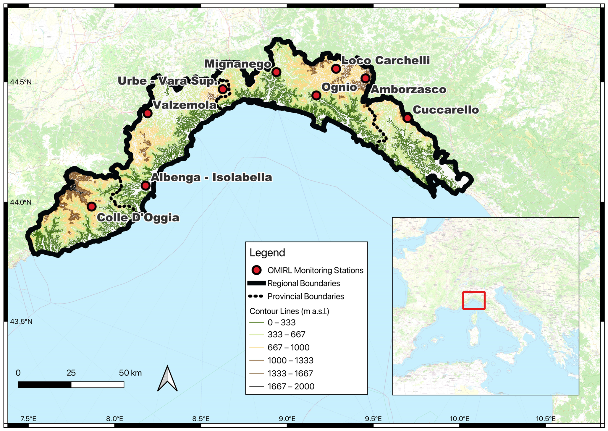
The ground network provides measurements from FDR sensors (model PCTUM011; MTX Srl, Campogalliano, Italy) at nine different locations (see the map in Figure 1). These stations cover both coastal and mountainous environments, with elevations ranging from 36 m a.s.l. (Albenga-Isolabella) to 1163 m a.s.l. (Colle D’Oggia). At each location, sensors are installed at three depths: 10, 20, and 40 cm. The FDR sensors measure the VWC within a range of 0% to 57%, with a manufacturer-specified accuracy of ±3%. These sensors are part of a broader operational meteorological monitoring system; the additional ancillary data collected at these stations (e.g., from thermometers and rain gauges) was used to support the manual and visual quality control of the recordings.
Prior to the comparison with the SM products, the point measurements were vertically aggregated into three representative layers: a first (Depth 1), directly corresponding to the 10 cm sensor. The second layer (Depth 2), which was computed as the arithmetic mean of the 10 and 20 cm sensors. Finally, a deeper profile (Depth 3), computed as a weighted average of the 10, 20, and 40 cm sensors. The specific weights are 0.3, 0.3, and 0.4, respectively.
The availability of in situ data is primarily influenced by varying station installation dates and localized sensor malfunctions during the 2021–2025 analysis period. While most stations became operational in autumn 2021, Mignanego was the last to come online in April 2023. Furthermore, because computing the Depth 2 and Depth 3 layers requires simultaneous valid observations from all involved sensors, any missing data propagates through the aggregation process. Consequently, prolonged periods of invalid measurements at specific depths—such as the 40 cm sensor at Loco Carchelli and the 20 cm sensor at Mignanego—significantly reduced the number of available aggregated daily records. For instance, while Loco Carchelli provides 1353 valid days for its Depth 1, data gaps reduce its deepest aggregated profile (Depth 3) to 958 days. Similarly, Mignanego exhibits 813 valid days at the surface, but only 399 and 307 valid days for Depths 2 and 3, respectively.
Moreover, it is worth noting that in situ data from specific stations, particularly Valzemola and Cuccarello, exhibit wider range of variation in deeper soil layers compared to the surface. This suggests suboptimal sensor calibration at those specific depths within the regional network.
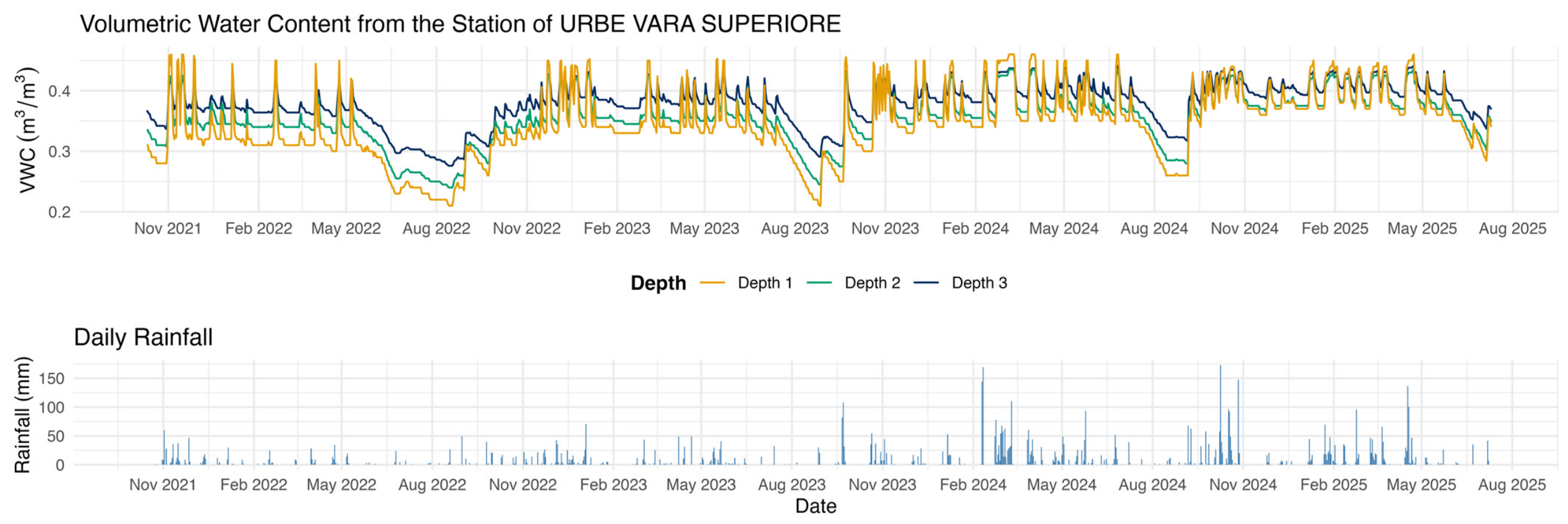
An example of the VWC aggregate time series recorded at the Urbe Vara Superiore Station is shown in Figure 2.

2.3.2. Continuum: Root Zone Soil Moisture

Continuum is a continuous, distributed and physically based hydrological model that [14] relies on a morphological approach based for the drainage network component identification [23]. The model solves energy and mass balance equations at an hourly timestep and a spatial resolution of ~200 m. The infiltration methodology is a modification of the Horton equation [24]. The RZ SM is modelled by considering a single layer, where each cell is represented as a tank with maximum storage volume Vmax [L] and a volume ad a certain time t that can be named V(t), and RZ SM at time t is expressed as shown in Equation (1):
R Z   S M t = V t V m a x   [ L 3 L 3 ] .
Table 2 provides an overview of the soil parameters and estimated root-zone depths for each study site. The soil information (Soil Type and Porosity) are extracted starting from the locations of each ground network station, which are subsequently used to estimate the root-zone depth values. A common Region of Interest (ROI) is defined according to the spatial characteristics of the dataset used for the analysis, such as HMC. The same ROI configuration is then applied to all ground stations associated with that dataset, ensuring a consistent spatial sampling procedure. For each station, the corresponding ROI is centred on its geographical location and used to extract the relevant soil properties from the SoilGrids dataset. The extracted values are subsequently associated with the corresponding monitoring station, providing representative soil information consistent with the spatial scale of the reference dataset. Soil data are obtained from SoilGrids, a global soil information system providing spatial predictions of soil properties at 250 m resolution [25].
A selective infiltration filter manages the water inflow, as shown in Equation (2):
g t = f 0 + f 1 f 0 V t V m a x [ L T 1 ] .
where f0 is the maximum infiltration rate under dry soil conditions, and f1 = c f f 0 is the minimum infiltration rate under saturated condition (RZ SM = 1). The field capacity of the soil is defined as V f c = c t V m a x , where ct [-] ranges from 0.2 to 0.6 and represents the mean field capacity. The parameter cf [-], varying between 0 and 1, is the infiltration capacity at saturation. V(t) is the level of storage volume at time t. Accordingly, the dynamic mass balance equation can be written as follows, where rp(t) denotes the percolation rate, assuming the condition V(t) > Vfc and r1(t) > g(t):
d V t d t = g t r p t = f 0 + f 1 f 0 V t V m a x V t c t V m a x V m a x 1 c t [ L T 1 ] .
More detailed description on the SM dynamics and the governing model equations are provided in [14] and partially reported in Appendix A while the model configuration adopted in this study follows an approach similar to that described in [22,26], but implemented at finer spatial and temporal resolution.

2.3.3. ECMWF: Root Zone Liquid Soil Water Index

The ECMWF Soil Moisture product used in this study is obtained by merging two datasets: (1) H142 and (2) the H26. Both of the datasets are outcomes from the Hydrology Tiled ECMWF Scheme of Surface Exchanges over Land (HTESSEL) Land Surface model [13], and the main distinction is that H26 is a Near Real-Time (NRT) product, whereas H142 is derived from ERA-5 reanalysis [27]. Differently, the atmospheric forcing for H26 is provided by the 9 km ECMWF IFS analysis. Merging these two datasets was necessary to cover the full period of analysis starting from June 2021.
Within the HTESSEL model, soil moisture is internally represented in volumetric units, but the final product is provided as Liquid Soil Wetness Index ranging from 0 (completely dry soil) to 1 (completely saturated soil). H142 and H26 rely on the Simplified Extended Kalman Filter (SEKF) assimilation system [28], which integrates ASCAT or SCAT sensors data. HTESSEL propagates soil moisture information in space and time, incorporating (1) orography, (2) soil texture data, (3) meteorological conditions and the (4) land surface processes [29,30].
One of the outputs of HTESSEL is the 10 km gridded Soil Liquid Wetness Index (RZ LSWI) profiles, provided daily for four soil layers: (1) Surface (0 cm) to 7 cm, (2) 7 cm to 28 cm, (3) 28 cm to 100 cm and (4) 100 cm to 289 cm.
In this study, only the upper soil layers were utilized. Specifically, the first layer (0–7 cm) and the first two layers were aggregated via a depth-weighted mean to compute an integrated 0–28 cm RZ LSWI profile.
The ECMWF product is derived from quality-controlled surface soil moisture observations through an infiltration model. Quality control is applied during the operational production chain, where observations affected by unfavourable retrieval conditions or failing the product quality criteria are excluded before the estimation of root-zone soil moisture. Consequently, no additional quality filtering was applied in this study beyond the standard quality assurance implemented by the data provider.

2.3.4. SMAP: Surface Soil Moisture

The National Aeronautics Space Administration (NASA) Soil Moisture Active Passive (SMAP) satellite mission [31,32] was launched in January 2015 with the objective of providing global high-resolution SM mapping based on L-band active (radar) and passive (radiometric) observations.
SMAP Level 2 (L2) products provide estimates of geophysical variables at the same resolution and location of the corresponding Level 1 product, within 24 h latency of acquisition. Specifically, L2SMP_E product [10,33] (version 6) used in this study provides gridded SSM estimates, representing the average VWC in the top 5 cm with retrieval times at 06 and 18 UTC. The SSM are obtained from the Backus–Gilbert interpolated radiometer brightness temperature [34] measurement at 9 km “enhanced” spatial resolution.
The SSM is estimated using passive microwave radiometry by measuring the brightness temperature measured at L-band frequency of 1.41 GHz. The variation in the emitted microwave radiation depends on the dielectric properties and temperature of the surface, which, for near surface soil layer, are strongly influenced by soil moisture content.
Brightness temperature observations from the SMAP enhanced Level 1 C [35] provide the primary input for the L2_SM_P_E product. The half-orbit granules are inspected for retrievability criteria according to input data quality, ancillary data availability, and land cover conditions [33]. Then, corrections are applied for surface roughness, effective soil temperature, vegetation water content, and the radiometric contributions by water bodies. Finally, the radiometric observation and ancillary data are used as inputs to the SMAP SSM retrieval algorithm.
In this analysis, the SMAP dataset was quality-controlled during the swath processing stage using the ancillary surface air temperature information distributed with the product. Observations acquired under freezing conditions (surface air temperature < 0 °C) were excluded from further processing to reduce the impact of frozen soil on the soil moisture retrievals.

2.3.5. ASCAT: Surface Soil Moisture

ASCAT is a real aperture radar system operating in C-Band (VV polarization) at 5.255 GHz, capable of providing measurements under all-weather condition and during nighttime. The instrument is onboard the MetOp satellites, which operate in a sun-synchronous orbit with an ascending node at 21:30 UTC and a minimum orbit height of 822 km, completing 14 orbits each day and providing a total daily coverage of about 82% of the globe [36].
The H16 soil moisture product is developed within the framework of the EUMETSAT Satellite Application Facility on Support to Operational Hydrology and Water Management (H-SAF) project. H16, a Level 2 SSM product provided in saturation degree, represents the topmost soil layer (<5 cm). It is derived from radar triplet backscattering coefficients (σ0) measured by the ASCAT antenna beams. Each σ0 measurement is given by the average of multiple radar echoes and produces SSM estimates with a spatial resolution of 25 km resampled to 12.5 km grids.
Soil moisture retrieval is based on a time series change detection approach developed by TU Wien University and described in [37]. The estimated surface soil moisture is expressed as percentage (0–100%), by scaling it between its minimum and maximum values registered on the specific pixel.
In this analysis, the ASCAT dataset is quality-controlled during the swath processing stage, before the observations are converted into the final gridded product. Each observation is screened using ancillary information describing the climatological probability of snow cover and frozen soil occurrence for each day of the year at every location. Observations are discarded when the probability of either snow cover or frozen soil exceeds 20%, ensuring that measurements acquired under environmental conditions known to degrade the accuracy of the ASCAT retrieval algorithm are excluded from further processing and subsequent analyses.

2.3.6. Point vs. Pixel Discrepancy

Modelled and satellite-based products provide spatially distributed data, while ground measurements represent point observations of VWC over time.
To enable a direct comparison, the distributed datasets were first extracted at the exact coordinates of each station for every available timestep. The geographical search is performed through the following steps:
  • Starting from the sensors point coordinates (longitude, latitude as in Table 2), the algorithm searches for the nearest grid cell of the dataset using a nearest-neighbour approach. The search is constrained by a maximum search radius (ROIgrid) of 12.5 km to ensure that the selected grid cell is representative of the target location.
  • Once the nearest grid cell has been identified, it is used as the centre of a 3 × 3 spatial window, defining the local neighbourhood to be analyzed.
  • All grid cells within the 3 × 3 window are evaluated, and only those whose centres lie within a second Region of Interest (ROIpoints) of 12.5 km from the target point are retained.
  • The values associated with the selected grid cells are then combined according to the chosen extraction strategy. The representative value for the point is obtained by computing the average of all valid grid cells located within the ROI to mitigate the impact of potential missing values in individual pixels.
This spatial aggregation reduces the influence of extreme or non-representative values within the distributed datasets (e.g., grid cells intersecting the drainage network in the case of the HMC where pixels might be fully saturated and unrepresentative of the surrounding soil).
However, in situ point measurements cannot fully represent pixel-scale soil moisture conditions (and vice versa). This spatial mismatch is particularly critical in the Ligurian Region due to its complex orography.
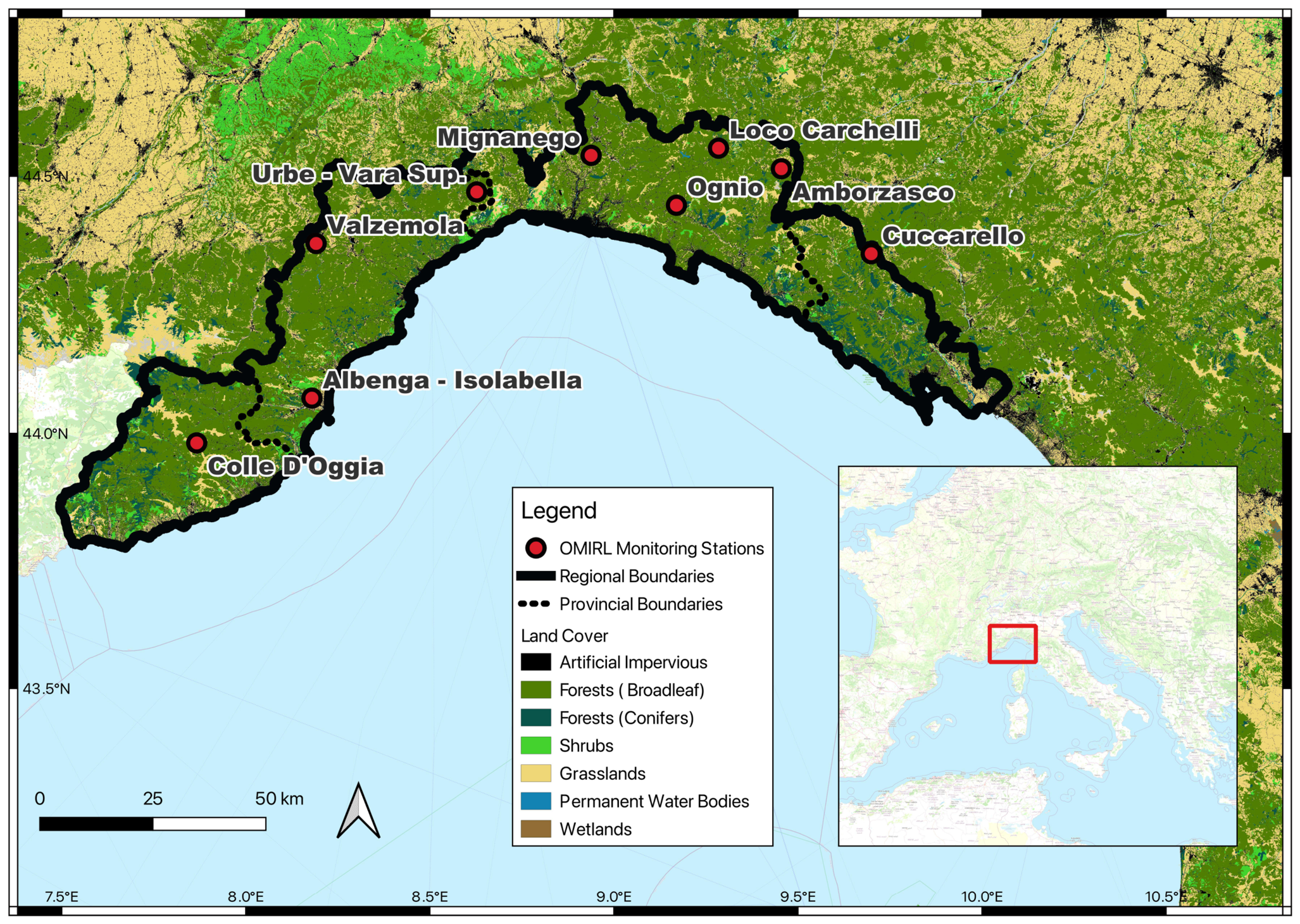
To provide a general overview of the environmental characteristics and quantify the potential heterogeneity within each product’s footprint, an external ancillary analysis was performed. Spatial statistics were extracted using circular buffers centred on each ground station. Under the assumption that these buffers can adequately approximate the spatial support of the respective grids, a radius of 12.5 km was hypothesized as representative of the coarse-resolution products’ (ECMWF, ASCAT, SMAP) 3 × 3 window footprint. Conversely, a 300 m radius was used to represent the footprint of the high-resolution HMC dataset. Within these defined buffers, elevation and land cover characteristics were extracted from a conditioned Digital Elevation Model (DEM) [38] and the ISPRA land cover dataset [39], to characterize the local heterogeneity of each footprint.
As reported in Table 3 the analysis highlighted significant spatial mismatch for coarse-resolution products. Within the 12.5 km circular buffers, the extraction area often encompasses extreme elevation gradients, sometimes ranging from sea level to nearly 2000 m a.s.l. within the same footprint. In contrast, the high-resolution HMC dataset significantly mitigates this issue, with elevation differences within its corresponding 300 m buffer typically remaining below 150 m.
While all nine in situ sensors are installed under an herbaceous layer, the extraction windows for coarse-resolution products are heavily dominated by broadleaf forests (60–85%). Conversely, the smaller HMC extraction windows capture greater local heterogeneity, better reflecting the specific herbaceous cover (up to ~50% at specific sites) alongside forested areas. Notably, Albenga Isolabella stands out by showing a significant fraction of artificial surfaces (approximately 30%), reflecting a more urbanized and fragmented landscape compared to the other predominantly natural sites. It is followed by Urbe Vara Superiore (~21%) Mignanego (~16%) and Valzemola (~15%). Despite these representativeness discrepancies, the goal of this analysis is to evaluate the capacity of the various rescaled products to capture the specific point-scale dynamics measured by the in situ sensors. To provide a visual representation of the spatial distribution of these land cover classes and their proximity to the evaluated monitoring stations, a detailed map (Figure A2) is provided in (Appendix B).

2.4. Methodology

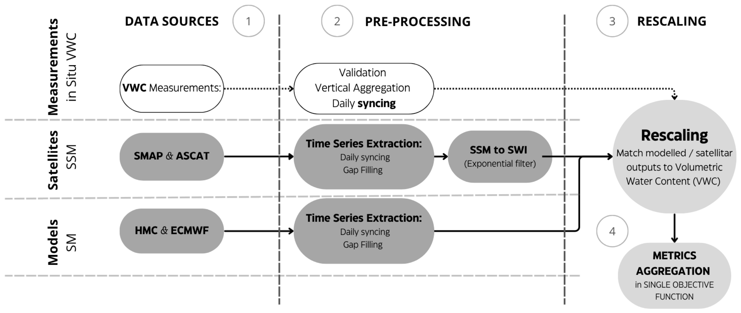
The SM products provide spatially distributed data describing the water quantity contained in the soil, using different physical quantities, sensing depths and spatial–temporal resolutions, while ground measurements represent point observations of VWC over time. To enable a direct comparison, the distributed datasets were first extracted at the exact coordinates of each station (as explained in Section 2.3.6) for every available timestep. Subsequently, all data series were synchronized to a daily resolution. Finally, an exponential filter, initially proposed by [37], was applied (Section 2.4.3) exclusively to the satellite-based products to generate the Soil Water Index (SWI). Subsequently, to mitigate systematic biases and enable direct comparison with ground-based measurements, five different rescaling techniques [40] were applied (Section 2.4.2). These specific methodologies were selected as they have been widely used in the previous literature [41,42,43]. The agreement between datasets was evaluated using standard statistical metrics (NSE, Pbias, and Pearson correlation), which were aggregated into a multi-objective function using a approach similar to that described in [44,45]. This function is formulated as a single scalar based on Euclidean distance, with offset terms introduced to balance the contribution of each metric. The workflow is summarized in Figure 3. Ultimately, the resulting performance of all datasets is summarized and visualized through heatmaps and Taylor Diagrams.
It should be noted that the same in situ dataset is used both as rescaling reference time series and for performance evaluation; therefore, the present analysis does not represent an independent validation, but rather a comparison of the consistency between the rescaled soil moisture products and their reference observations.

2.4.1. Data Preprocessing

Since temporal resolution depends on satellite revisit time, swath geometry, and model run schedules, all products are resampled to a daily timestep using a forward moving average window. Then, a gap-filling procedure based on polynomial interpolation is applied to the time series only when missing data spans a maximum of two consecutive days.
The depth mismatch between in situ measurements and SM products was addressed by matching specific model-satellite layers exclusively with their most consistent in situ aggregation depth. Specifically, the ECMWF 0–7 cm surface layer was compared with Depth 1 while the ECMWF 0–28 cm layer was compared with Depth 2 Conversely, the RZ SM from Continuum (which lacks a fixed nominal depth) and the SWI-filtered satellite products were evaluated across all three aggregated in situ depths to investigate which vertical profile yielded the optimal agreement.
Finally, all subsequent rescaling procedures and statistical evaluations were performed exclusively on temporally collocated data. This means that data pairs were retained only for timesteps where both the in situ observation and the corresponding modelled or satellite product were simultaneously available.

2.4.2. Rescaling Techniques

To reduce systematic biases between satellite-based, model-based, and in situ soil moisture measurements, it is common practice to filter and/or to rescale the SM products against a reference dataset [40,46].
In the following equations, for a given station and reference depth, e t represents the soil moisture product value at time t, e t s c a l e d the rescaled value, and o t is the corresponding aggregated in situ VWC observation. e ¯ and o ¯ are the sample means of the series, respectively, of the SM product and of the VWC series, respectively, s o and s e denote the standard deviations. All products were rescaled and expressed in the units of the reference observations, namely VWC (m3 m−3).
In this study, the following rescaling methods were applied:
  • Min-Max stretching (min_max) adjusts the minimum and maximum values of the SM product to match those of the reference time series, preserving the relative variability of the original data applying Equation (4).
e t s c a l e d = m a x o m i n o m a x e m i n e · e t m i n e + m i n o .
  • The linear regression (linreg) method estimates the coefficients a and b of the linear model in Equation (5) by minimizing the sum of squared errors between the reference series and the SM product.
e t s c a l e d = a e t + b .
  • The linear rescaling (mean_std) approach normalizes the series by matching its mean and standard deviation to those of the in situ reference, applying Equation (6).
e t s c a l e d = s o s e · e t e ¯ + o ¯ .
  • The Cumulative Distribution Function (CDF) matching techniques are used to minimize the systematic errors between different datasets by matching the Empirical Cumulative Distribution Functions (ECDFs) of the target and reference datasets. This ensures that the rescaled SM value correspond to the reference VWC associated with the same Cumulative probability. In this study, two ECDF interpolation methods were explored: (1) linear interpolation (lin_cdf_match or linear CDF matching) and (2) Beta function interpolation (cdf_beta_match or CDF Beta Matching).

2.4.3. Soil Water Index (SWI)

Prior to the scaling process, satellite-based products are appropriately filtered. While various temporal filters exist, such as the Moving Average Filter [47] and the Boxcar Filter, this study employs the exponential filter. Specifically, a simple estimation of the average profile SM at deeper layers is performed by applying the SWI [37] to the satellite-derived surface measurement (ASCAT and SMAP) using the recursive formulation of Equation (7):
S W I t n = i = 0 t n S S M t i e t n t i / τ i = 0 t n e t n t i / τ ,
where τ is the characteristic time length expressed in days. Higher values of τ produce a stronger smoothing and delaying effect on the input SSM signal, thereby mimicking soil moisture conditions in deeper layers.

2.4.4. Performance Evaluation

To assess the agreement between the rescaled and the reference time series, statistical performance metrics were computed. The evaluation was based on the following metrics: The Nash–Sutcliffe Efficiency (NSE) with Equation (8):
N S E = 1 t = 1 T o t e t s c a l e d 2 t = 1 T o t o ¯ 2 = 1 M S E σ o 2
  • The Percent Bias (Pbias) is computed with Equation (9):
P b i a s = t = 1 T e t s c a l e d o t 100 o t .
  • The Pearson R or correlation coefficient (CC) is computed with Equation (10):
CC = t = 1 T o t o ¯ e t scaled e scaled ¯ t = 1 T o t o ¯ 2 t = 1 T e t scaled e scaled ¯ 2 .
where e t s c a l e d represents the general rescaled SM product [m3 m−3] at time t, o t is the reference VWC [m3 m−3] value at time t. Furthermore, e ¯ ,   e s c a l e d ¯   a n d   o ¯ are the sample means of the respective time series.
The individual objective functions F 1 θ ,   F 2 θ ,   F 3 θ correspond to the adapted performance metrics reformulated for minimization, as follows:
F 1 θ = P b i a s 100 ;   F 2 θ = C C ;   F 3 θ = N S E .
θ denotes the decision variable in the feasible parameter space Θ, identifying the combination of the rescaling method and the SWI time length τ, such that
θ = r , τ Θ = R × T ,
with
R = { m i n _ m a x , l i n r e g , c d f _ b e t a _ m a t c h , l i n _ c d f _ m a t c h , m e a n _ s t d }
representing the set of rescaling methods, and
T = { 0   d a y s ,   1   d a y s ,   2   d a y s ,   60   d a y s }
representing the set of time lengths (where τ = 0 days corresponds to no exponential filtering).
Subsequently, similarly to what was proposed in [44], the three objective functions were equally weighted and aggregated into the multi-objective function F a g g θ , defined as a scalar based on the Euclidean distance:
F a g g θ = F 1 θ + A 1 2 + F 2 θ + A 2 2 + F 3 θ + A 3 2 1 2 ,
In this formulation, the offset terms Ai, are introduced to ensure that the shifted components ( F i θ + Ai) maintain a comparable distance from the ideal origin across all metrics. These terms are pre-calculated as constants prior to the evaluation of the multi-objective function, defined as follows:
A i = m a x F 1 , m i n , F 2 , m i n , F 3 , m i n F i , m i n ;
where Fi, min represents the global minimum achieved by the i-th objective function across the entire feasible parameter space Θ :
F i , m i n = min θ Θ F i θ , i = 1 , 2 , 3
This formulation ensures a balance contribution of each objective function, so that no single metric dominates the aggregated score.

2.4.5. Taylor Diagrams

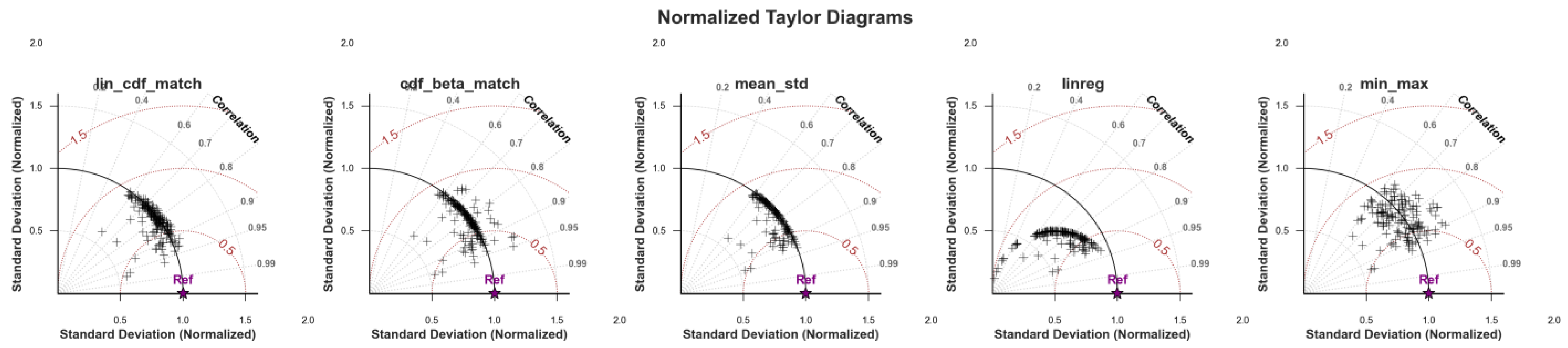
In the Section 3, Taylor diagrams [48] are employed to visually evaluate the relative performances of the rescaled SM datasets. Since the unbiased root mean square error (ubRMSE) [49], the standard deviations, and the correlation coefficient (CC) are geometrically linked, they can be simultaneously displayed on a concise two-dimensional plot.
To allow for a direct comparison across different monitoring stations, the results are visualized using Normalized Taylor Diagrams, meaning that statistical metrics are divided by the standard deviation of the corresponding in situ reference series.
The reference dataset is placed on the x-axis at a normalized standard deviation of 1 and a correlation coefficient of 1 and is indicated by a violet star marker. The location of each point is determined by its normalized standard deviation (radial coordinate) and its correlation coefficient with the reference dataset (angular coordinate), while the normalized ubRMSE is inferred from its distance to the reference marker. Specifically:
  • The normalized standard deviation is represented by the radial distance from the origin to a given point. The solid black arc at a radial distance of 1 represents the normalized standard deviation of the reference dataset (Ref).
  • The CC with the reference is represented by the angular coordinate of a point, with dotted radial lines indicating specific correlation values.
  • The normalized ubRMSE can be inferred from the distance between the reference marker and a dataset’s point, with dashed brown isolines.
Overall, points located closest to the violet marker indicate the highest level of agreement, ideally combining high correlation, low ubRMSE, and a standard deviation comparable to that of the reference.

3. Results

The performance metrics are calculated by comparing the vertically aggregated in situ measurements against the rescaled (and/or filtered) product time series. This procedure of rescaling is applied under the assumption that it mitigates the inherent point-to-pixel discrepancies (e.g., in situ sensors are locally installed under an herbaceous layer, whereas the grid cells of the evaluated products, particularly the coarser ones, often encompass highly heterogeneous landscapes with significant forest fractions).
For the sake of conciseness, specific result sections focus on a representative two-year sub-period (July 2023–July 2025) rather than the full four-year window (July 2021–July 2025). While absolute metrics vary between the two durations, the general findings and the relative performance of the products remain consistent across both timeframes. The specific differences and the performance degradation observed when considering the entire four-year period are explored in greater detail in Section 3.2. Furthermore, the specific analyses presented in Figure 4 and Figure 5 for the two-year timeframe have been replicated for the full four-year period; these extended results are provided in Appendix C (Figure A3 and Figure A4).

3.1. SWI: Identifying the Optimal τ

The SWI, as previously described in Section 2.4.3, was computed from the satellite-based SSM time series prior to the application of any rescaling procedures. Sixty τ values were tested (τ = 1, 2, 3, …, 60 days) across all the measurement sites and reference depths. The primary aim was to identify the individual τ value capable of providing the best overall agreement with the in situ series (i.e., minimizing the multi-objective function).
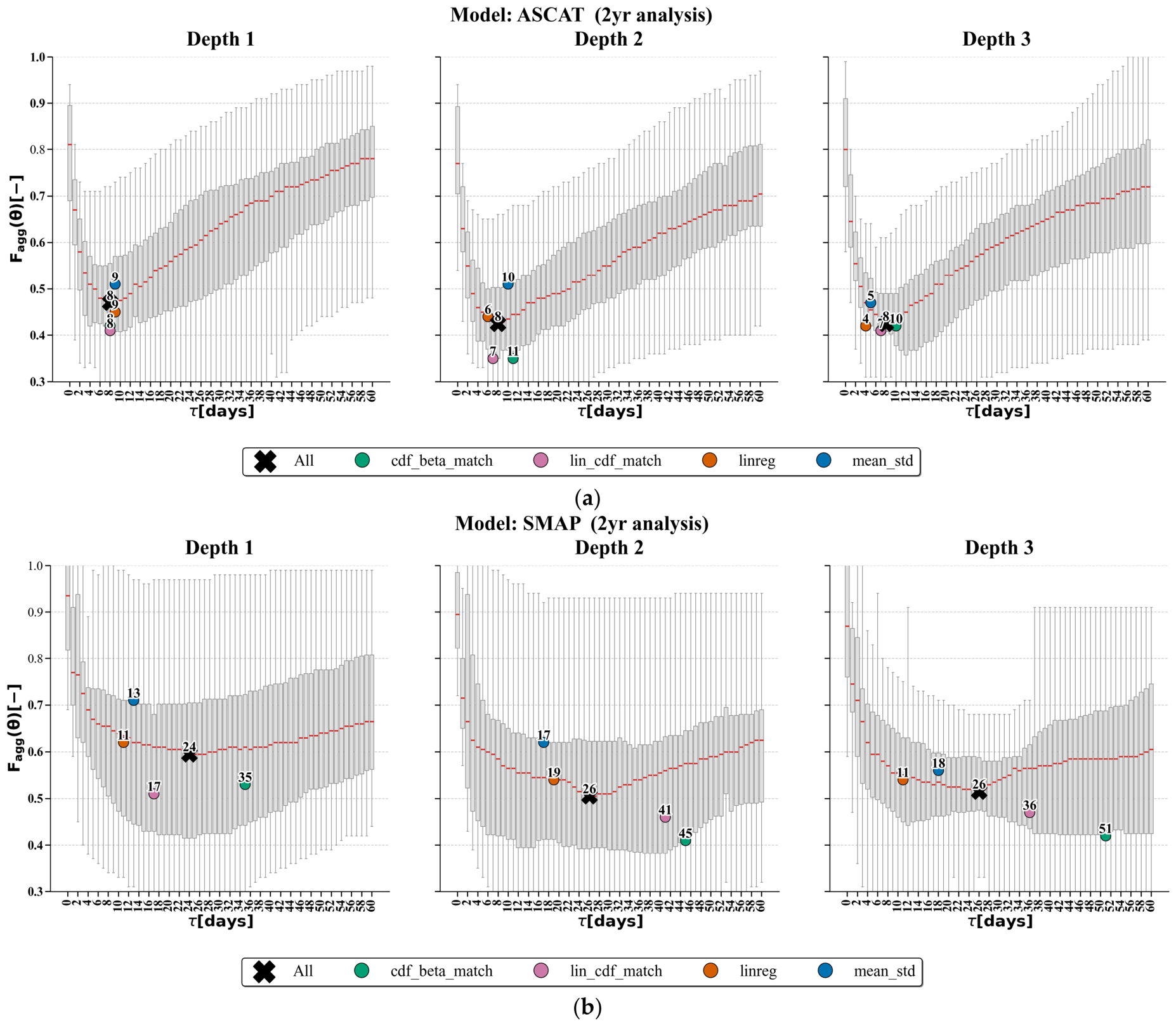
Figure 4 illustrate the results of this sensitivity analysis for ASCAT and SMAP product presented as boxplots.
For ASCAT, the multi-objective function exhibits a well-defined minimum for exponential filter times length (τ) ranging from 4 to 11 days across all depths (Figure 4a). When evaluating the median performance across all aggregated rescaling methods (denoted by the “All” marker), the optimal τ is found to be constant with soil depth: 8 days for Depths 1, 2, and 3, respectively. Furthermore, the optimal τ values identified for the different rescaling techniques cluster relatively close to one another. This suggests that the choice of the optimal τ parameter exerts a stronger influence on the overall performance than the specific rescaling method adopted.
Conversely, the analysis for the SMAP product, shown in Figure 4b, reveals a distinctly different behaviour compared to ASCAT. When examining the aggregated median performance (the “All” marker), the optimal characteristic time length is found at 24, 26, and 26 days for Depths 1, 2, and 3, respectively. Unlike the ASCAT results, SMAP requires significantly higher τ values. Furthermore, unlike the well-defined minimum observed for ASCAT, the SMAP objective function exhibits a broad and nearly flat valley across all depths. Because a clear, minimum is absent, the optimal τ values identified for the individual rescaling methods are highly dispersed. For instance, at Depth 1, τ ranges drastically from 11 days (linear regression) to 35 days (CDF Beta Matching). Indeed, the optimization of the temporal filter is highly sensitive to the specific rescaling technique.
Overall, comparing Figure 4a,b indicates that the optimal filtering time is product-dependent. This suggests that the inherent characteristics of ASCAT and SMAP retrievals differ significantly, thereby requiring different levels of temporal smoothing prior to comparison within situ observations.
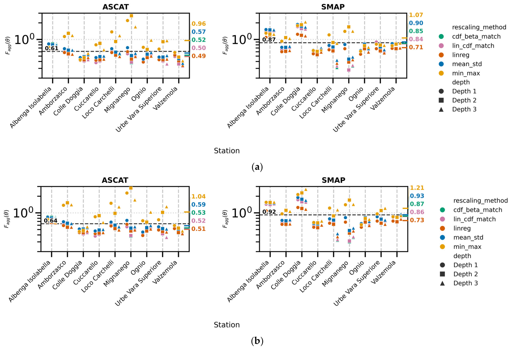
Two τ calibration strategies were compared: site-and-depth-specific optimization (optimal τ for each combination) and a product-specific approach (τ = 8 days for ASCAT; τ = 25 days for SMAP). As shown in Figure 5, adopting a generalized τ for specific products (panel b) introduces only marginal performance degradation compared to specific calibration (panel a). These results indicate that more robust rescaling techniques (both CDF matching techniques, linear regression and linear rescaling) effectively compensate the lack of site-specific τ optimization. However, Min-Max stretching represents a notable exception, exhibiting significant deterioration when non-optimal τ values are applied.
After excluding Min-Max stretching and instances where the rescaled product lacked skill even with local optimization (NSE < 0 or R < 0), the maximum performance degradation was assessed. In worst-case scenarios, specifically at the Colledoggia station across all depths, the decreases in NSE and R were constrained within 0.14 and 0.07, respectively. While these cases exhibited a maximum increase in the Fagg of approximately 0.24, they represent isolated outliers.

3.2. Comparison over Different Products, Station Sites and Rescaling Methods

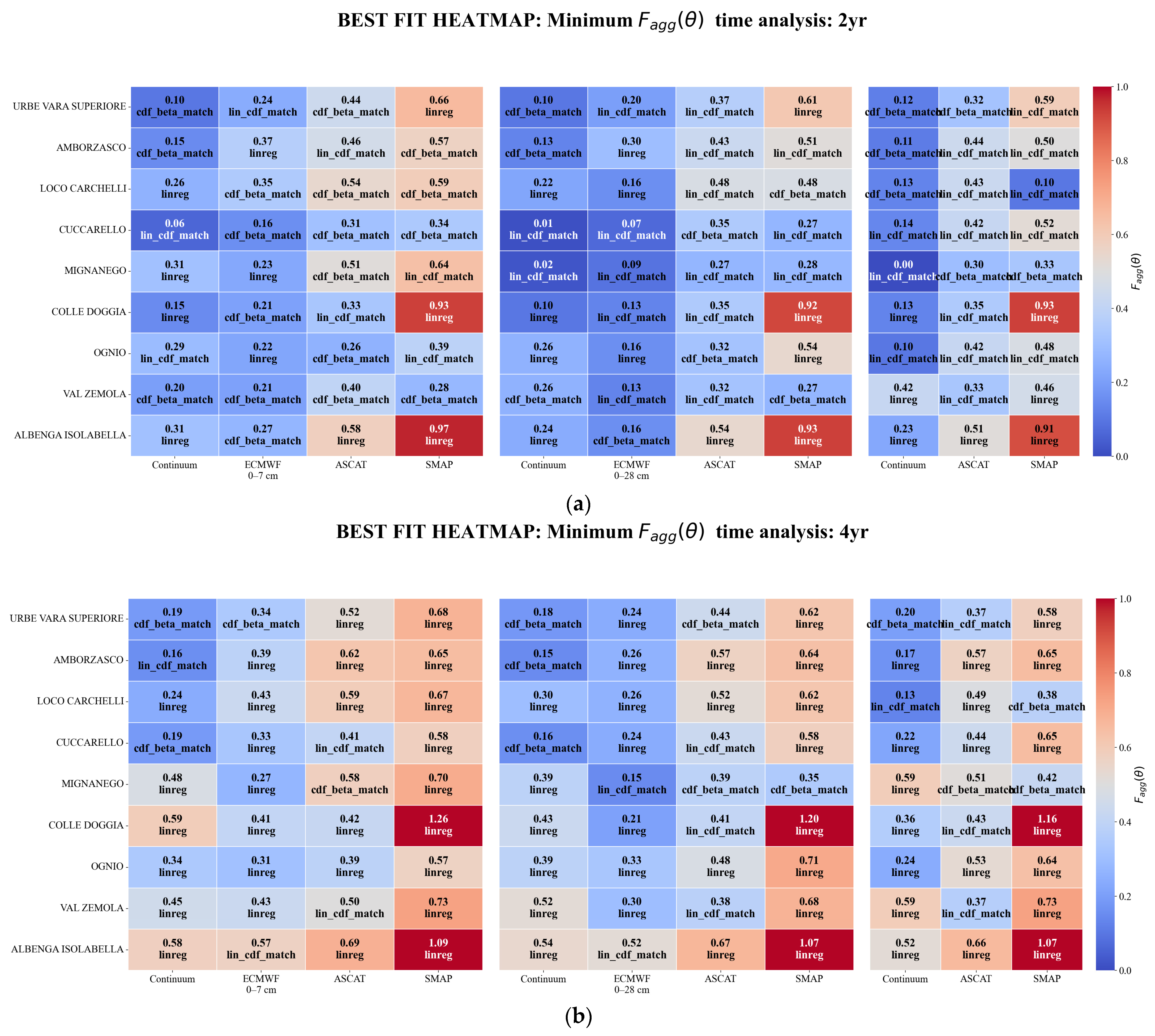
The heatmaps in Figure 6 illustrate the evaluation results for two distinct time windows: a restricted two-year period (July 2023–July 2025, panel a) and an extended four-year period (July 2021–July 2025, panel b). This dual evaluation stems from a noticeable performance degradation observed over the longer period, which includes the severe multi-year drought that affected Italy between late 2021 and mid-2023 [50]. This extreme climatic anomaly distorted the statistical rescaling process, leading to systematic overestimations during dry spells and underestimations during wetter periods. By excluding this extreme event, the restricted two-year analysis effectively mitigates these biases, systematically yielding higher accuracy—indicated by lower Fagg values and bluer shades, compared to the full four-year period.
Focusing on the effectiveness of the rescaling methods during the optimal two-year period (panel a), CDF matching emerges as the most robust rescaling strategy overall. Among its implementations, CDF matching with linear interpolation (lin_cdf_match) minimizes the multi-objective function in 37 out of 99 evaluated combinations, while CDF matching with Beta function interpolation (cdf_beta_match) achieves the lowest Fagg values in 31 cases. Linear regression (linreg) exhibits comparable performance, also emerging as the optimal solution in 31 combinations.
A different pattern emerges in the four-year analysis (panel b), where linear regression becomes the most frequently selected method, yielding the lowest Fagg values in 68 out of 99 combinations. However, cross-referencing this result with the Normalized Taylor Diagrams (Figure 7) reveals a limitation of this technique. As shown in the specific subplot (orange markers), while linear regression effectively reduces the ubRMSE, it systematically underestimates the natural variability of the datasets. All-time series rescaled via linear regression are compressed well inside the solid black reference arc, indicating a normalized standard deviation of the reference dataset.
It is important to note that the notably higher performance metrics obtained for Loco Carchelli (Depth 3) and Mignanego (Depths 1 and 2) should be interpreted with caution. These improvements are most likely attributable to an overfitting effect, driven by the significantly shorter time series available for these specific depths compared to the other stations in the network.
Table 4 summarizes the median values and inter-station standard deviation for ubRMSE, CC, and Fagg across the three investigated depths, with a specific focus on the linear CDF matching and linear rescaling techniques. For these two methods, the ubRMSE is equivalent to the RMSE, as they effectively eliminate systematic bias (unlike the Min-Max stretching approach). Linear rescaling was included primarily to ensure that intrinsic product dynamics remain undistorted; unlike CDF matching, which may inadvertently alter correlation metrics when applied to limited datasets, linear rescaling preserves the original Pearson correlation. Consequently, while this approach may yield slightly lower performance scores—such as higher ubRMSE and decreased NSE—it provides a more transparent baseline for evaluating the rescaled products. Based on these results, model-based products (Continuum’s and ECMWF 0–28 cm) consistently outperform satellite-derived estimates across all depths, exhibiting lower absolute errors (ubRMSE ranging from 0.015 to 0.030 m3/m3). While Continuum is slightly more accurate at the shallowest layer (Depth 1) than other products, the 2-year window analysis reveals improved performance at Depths 2 and 3 (except for Valzemola, probably due to sensor calibration issues). This improved performance, reflected in lower ubRMSE at greater soil depths, aligns perfectly with the estimated RZ depths (ranging from 18 to 35 cm, Table 2). Similarly, ECMWF shows a marked improvement at Depth 2, matching Continuum’s accuracy and achieving the highest overall correlation (CC = 0.890). Regarding satellite retrievals, ASCAT systematically provides more reliable estimates than SMAP, which is penalized by higher errors and larger spatial variability. Furthermore, a distinct vertical pattern emerges: ASCAT exhibits an optimal performance at the Depth 2. SMAP also shows vertical improvement, with estimations at Depths 2 and 3 consistently reporting lower ubRMSE and Fagg values, coupled with higher CC and NSE compared to Depth 1. Finally, substituting station- and depth-specific optimized filtering parameters (τopt) with fixed, product-specific ones (τ = 8 days for ASCAT and τ = 25 days for SMAP) introduces only a marginal performance degradation.

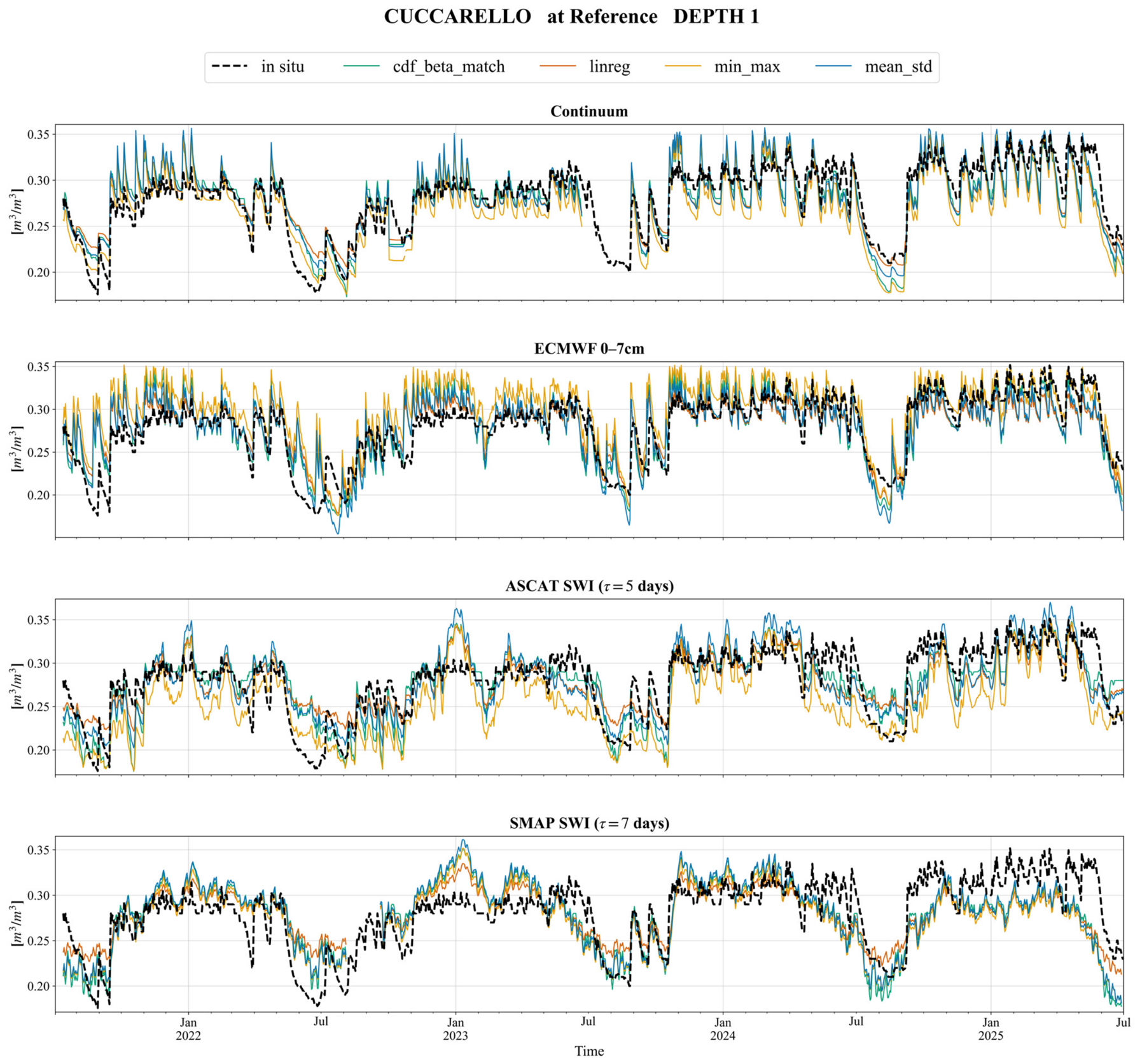
3.3. Test Case: Cuccarello Station

Figure 8 and Table 5 present a subset of the four-year analysis for the Cuccarello station (Depth 1), evaluating four SM products across four rescaling techniques. Despite site-specific variations, three consistent trends emerge from this configuration. First, regarding the rescaling procedures, Min-Max stretching systematically yields the poorest performance (highest biases and Fagg scores). Second, rescaled model-based products (particularly Continuum) generally outperform satellite retrievals, achieving higher correlations (CC > 0.85, NSE > 0.71) and lower overall errors. Finally, within the remotely sensed category, ASCAT consistently demonstrates superior agreement with in situ measurements compared to SMAP.

4. Discussion

This study presented a comparative analysis of two satellite-based SSM products (ASCAT and SMAP) and two model-based soil moisture products (HTESSEL and Continuum). The evaluation focused on their coherence with in situ measurements from the Ligurian Meteo-Hydrological Observatory, the effectiveness of different rescaling methods in reducing biases, and the impact of sampling periods on the final coherence. Based on the analysis, the main conclusions can be summarized as follows:
  • Model-based rescaled soil moisture products generally outperformed satellite-based estimations in terms of coherence with in situ VWC measurements. Specifically, the Continuum root-zone soil moisture and the ECMWF at 0–28 cm depth products achieved the best performance. Notably, despite its coarser spatial resolution, ECMWF effectively captures soil moisture at sensor depths, likely due to its layered soil representation.
  • While ECMWF performance is inherently linked to ASCAT due to data assimilation, the model consistently outperforms the satellite product across all monitoring sites. This suggests that the integration of meteorological forcings (e.g., precipitation and temperature) and the physical modelling of soil water dynamics effectively filter the noise typical of raw satellite signals.
  • The degree of coherence varies according to the specific combination of station, depth, and product, often without exhibiting a distinct overall spatial pattern. However, specific sites, such as Albenga Isolabella and Colle D’Oggia, consistently emerge as systematic upper outliers across multiple depths. These locations exhibit particularly high discrepancies, especially in satellite-derived SWI SMAP estimation. These errors are likely driven by topographic complexity, dense forest cover and anthropogenic land use, which amplify retrieval uncertainties. For instance, the extreme elevation variance within coarse satellite footprints (e.g., ranging from 38 to 2090 m within the 12.5 km circular buffer at Colledoggia) introduces severe sub-pixel heterogeneity, thereby degrading the retrieval accuracy. At Albenga Isolabella, the substantial fraction of artificial impervious surfaces (~30% within a 300 m circular buffer) combined with its coastal proximity likely introduces significant radiometric noise into the satellite signals. The two model products (Continuum, HTESSEL) also evidence quite good performance for Albenga Isolabella and Colledoggia, probably because the physical description of soil moisture dynamic through meteorological forcing is less affected by the presence of urban areas interspersed with natural areas than satellite imagery.
  • Despite these specific site-level observations, looking at the results and at Table 3, it does not seem easy to directly relate the results in every case (e.g., Figure 6) with the terrain characteristics (land use, vegetations, …). As previously noted, the percentage of artificial surface can explain non-performing score values in ASCAT and SMAP products for Albenga Isolabella but not for Colledoggia. Moreover, the coarse resolution that causes various types of conditions to be averaged in each grid pixel creates difficulties in interpreting results and makes it difficult to pursue rigorous analysis, as comparing these footprints (>10 km) with limited point-scale measurements [32] remains a major, unavoidable source of uncertainty in such a highly heterogeneous landscape.
  • In a broader context, the lower agreement of SMAP with in situ observations in the densely vegetated Ligurian study area is consistent with the findings of [9,51], which generally report better performance in sparsely vegetated environments than in regions characterized by dense vegetation cover.
  • The lower performance observed for the satellite-based products in this study highlights the challenges faced by microwave soil moisture retrievals in topographically complex and densely vegetated areas (steep terrain, densely vegetated cover, …) [8,52].
  • Consistent with [40], CDF matching (cdf_beta_match and lin_cdf_match) proved to be the best-performing technique among the tested approaches, outperforming both linear rescaling and Min-Max stretching. Moreover, linear regression remains an effective method for reducing biases; it tends to consistently underestimate the temporal variability of the rescaled SM products compared to the reference time series.
  • Regarding the estimation of SM at deeper layers from satellite SSM, the implementation of an exponential filter, following methodologies also used in other Mediterranean catchments [53], allowed for the derivation of the Soil Water Index (SWI). By calibrating the τ parameter against in situ measurements, our analysis identified optimal τ values for ASCAT between 7 and 8 days for depths ranging from 10 to 40 cm. This range appears comparable to the τ value of 9.5 days optimized for measurements obtained at a 25 cm sensor depth reported in the aforementioned study [53], suggesting a general agreement in the parameter’s behaviours within similar Mediterranean environments.
  • Shortening the time window analysis from 4 to 2 years improves the agreement between the reference and rescaled time series.
  • The application of product-specific τ values for satellite products does not lead to an excessive deterioration in statistical scores compared to locally calibrated parameters. Similar conclusions specifically for ASCAT were also found in [46].
The findings of this study are inherently case-dependent, relying on a limited number of stations and observation years. Furthermore, the analysis is subject to uncertainties arising from depth mismatches between modelled products and in situ sensors, as well as the inherent grid-to-point scale discrepancy between pixel-scale SM products and point-scale VWC measurements. For example, all in situ sensors are installed under herbaceous vegetation, whereas the corresponding pixels—particularly for the coarser-resolution products—are generally dominated by broadleaf forests. Although these scale mismatches represent a recognized source of uncertainty, the evaluation of spatially and temporally aggregated products against point-scale in situ observations remains widely adopted [7,8,9,51]. An additional source of uncertainty in the overall assessment arises from suspected sensor calibration problems. Nevertheless, this empirical approach remains a valuable framework for assessing the capability of specific soil moisture products to capture the specific local ground conditions.
Comparison results can be potentially used in a near real-time framework to evaluate variabilities of the different soil moisture estimations, since soil moisture is a key topic in flood forecast. It could help forecasters to understand and interpret the discrepancy between the various products and make them conscious that comparison with in situ measurements does not have the same reliability for all sites. Moreover, since considered products have low latency, it is possible to adapt some of the comparison procedures presented so that they can be updated on a daily or sub-daily basis and to assess the consistency between on-site and remote estimates over the most recent period.
From a scientific point of view, this study could be explored in greater depth, for example by analyzing any additional information derived from a more detailed analysis of land use as described by the various systems under consideration. It should be noted, however, that the different spatial resolutions, which are sometimes rather coarse (e.g., 9–12.5 km), could introduce further uncertainty into the interpretation of the results, particularly given the complex topography of the study area.
To mitigate this spatial mismatch, it is acknowledged that more rigorous validation methods could be employed. These could include the spatial downscaling of SM products [54,55] using high-resolution ancillary data, or the upscaling of point measurements by deploying multiple sensors within a pixel [32] footprint, where possible. Nevertheless, the implementation of such procedures falls outside the scope of this specific analysis.
Future developments could explore time-varying calibration coefficients within the rescaling procedure [56,57] as well as applying the SWI recursive formulation, as described in [58], and used in numerous studies [59,60,61].
Furthermore, regarding spatial sampling, analyses could consider extracting SM values from the coarser-resolution products (~9–12.5 km) by selecting only the pixel value closest to the station coordinates [46,62], rather than using a 3 × 3 pixel window.

Author Contributions

Conceptualization, L.R. and F.S.; methodology, F.D. and L.R.; software, F.D.; validation, L.R., F.S. and G.B.; formal analysis, L.R.; investigation, L.R., F.D. and F.G.; resources, F.S.; data curation, F.D. and F.G.; writing—original draft preparation, L.R.; writing—review and editing, L.R., F.D., F.S. and G.B. All authors have read and agreed to the published version of the manuscript.

Funding

This research was funded by the Regional Agency for Environmental Protection of the Liguria Region (ARPAL, 8 Bombrini Street, Italy, Genova, Tax ID Code: 0130593010) through an agreement between ARPAL and the CIMA Research Foundation, for the activation of useful synergies in the field of forecasting, prevention, and monitoring of natural risks for the purposes of civil protection and environmental and biodiversity issues. The agreement cover the period 2019–2027.

Data Availability Statement

The data presented in this study are available on request from the corresponding author.

Acknowledgments

The authors acknowledge the providers of soil moisture datasets for the availability of the observations/estimations that made this comparison possible. ChatGPT–5 (OpenAI) and Google Gemini 1.5 were used to improve language clarity and assistance in script development. The authors have reviewed and edited the output and take full responsibility for the content of this publication.

Conflicts of Interest

The authors declare no conflicts of interest.

Abbreviations

The following abbreviations are used in this manuscript:
ATBDAlgorithm Theoretical Basis Document
ASCATAdvanced Scatterometer
ARPALAgenzia Regionale per la Protezione dell’Ambiente Ligure
CFMI-PCCentro Funzionale Meteo Idrogeologico di Protezione Civile
CDFCumulative Distribution Function
ECDFEmpirical Cumulative Distribution Function
ECMWFEuropean Centre for Medium-Range Weather Forecasts
ERSEuropean Remote Sensing
ESAEuropean Space Agency
EUMETSATEuropean Organization for the Exploitation of Meteorological Satellites
FDRFrequency Domain Reflectometry
HMCHydrological Model Continuum
H-SAFSatellite Application Facility on Support to Operational Hydrology and Water Management
HTESSELHydrology Tiled ECMWF Scheme of Surface Exchanges over Land
METOPMeteorological Operational Satellite Program
OMIRLMeteorological and Hydrological Observatory of Liguria
RMSERoot Mean Square Error
ROIRegion of Interest
RZRoot Zone
RZ LSWIRoot Zone Liquid Soil Water Index
SEKFSimplified Extended Kalman Filter
SMSoil Moisture
SMAPSoil Moisture Active Passive
SSMSurface Soil Moisture
SWISoil Water Index- Soil Wetness Index
TDRTime Domain Reflectometry
ubRMSEunbiased Root Mean Square Error
U.O. CMIUnità Operativa Centro Meteo Idro
VWCVolumetric Water Content

Appendix A. HMC–Subsurface Flow and Evapotranspiration

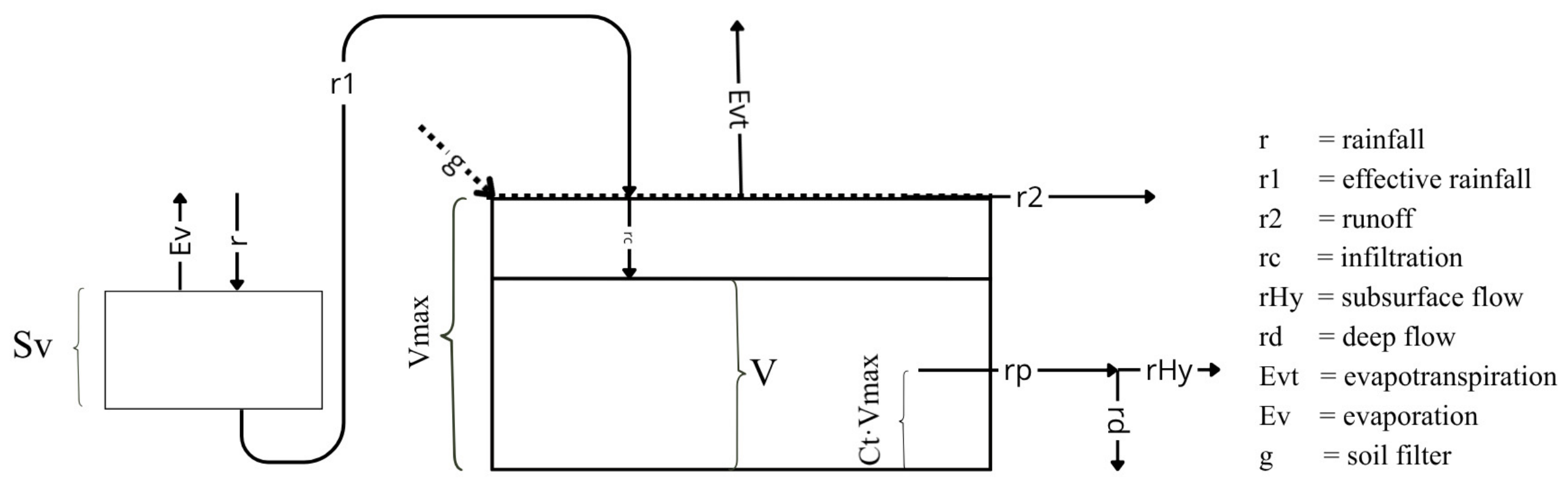
The infiltration scheme of Continuum model, illustrated in Figure A1, has four parameters. Specifically, the parameters f0 and Vmax are related to soil type and land use through the spatially varying curve number (CN), while ct and cf are assumed to be constant for whole river basins.
Figure A1. Infiltration and interception scheme of the Continuum Hydrological Model at cell scale, extracted from [14]. Sv is the capacity of the vegetation reservoir, Vmax the capacity of the soil reservoir, V the actual water volume in the soil and ct·Vmax the field capacity of the soil.
Remotesensing 18 02903 g0a1
The percolation rate rp [LT−1] is defined as the sum of the subsurface flow (rHy) and the deep flow (rd) recharging the water table. In particular, the subsurface flow propagates following the surface drainage directions. Consequently, the RZ SM of each cell is updated by accounting for both inputs: local infiltration and inflow from the upstream cells.
r H y = s i n α r p ( t )
rHy is defined in Equation (A1) as function of the decomposition term sin(α). Where α is defined such that tg(α) is the downslope index [63] and reproducing the major proneness of the high slope areas to subsurface flow due to gravity.
The subsurface flow mass balance equation is defined by (A2) where r1(t) is obtained by the sum of the net rain (rain depleted by vegetation interception) and of the upstream overland flow.
d V d t = r 1 t ; for   V t c t   V m a x   and   r 1 t g ( t ) d V d t = r 1 t f 1 V t c t V m a x V m a x 1 c t ; for   V t > c t V m a x   and   r 1 t g ( t ) d V d t = f 0 + f 1 f 0 V t V m a x ; for   V t c t   V m a x   and   r 1 t > g ( t ) d V d t = f 0 + f 1 f 0 V t V m a x f 1 V t c t V m a x V m a x 1 c t for   V t > c t   V m a x   and   r 1 t > g ( t ) .
As consequence the run-off is defined as:
r 2 t = r 1 t g t ; for   r 1 t > g t   0 for   r 1 t g t
The evapotranspiration ET [ms−1] and the interception storage Sv [L] are defined as:
E T = L E ρ w λ L E   a n d  
S v = 0.95 + 0.5 L A I 0.06 L A I 2 ,
where ρw [m L−3] is the water density, LE is the latent heat, λLE [E m−1] is the latent heat of vaporization and LAI is the Leaf Area Index usually updated every 15 days from optical sensor data (e.g., MODIS). ET is deducted from the interception storage Sv [L] if not empty, otherwise from the subsurface reservoir V(t) adding the following terms to Equation (A3) as follows:
d S v / d t = E T i f   S v > 0 d V / d t = E T i f   S v = 0
More detailed information about the energy balance equation, the deep flow and water table dynamics are described in [14] both in the main text and the appendix. Inputs needed for evapotranspiration estimation are: air temperature, solar incoming shortwave radiation, wind speed, and relative air humidity. They are derived by the CFMI-PC operational ground network (https://omirl.regione.liguria.it/ (accessed on 15 April 2026)). They are used to estimate the various terms of energy balance, as latent heat, sensible heat and the force restore equation which describes the daily cycle of land surface temperature.

Appendix B. Land Cover Map of the Study Area

This appendix provides additional geographical context regarding the environment surrounding the selected monitoring stations. Figure A2 illustrates the detailed spatial distribution of the land cover classes across the Liguria region, based on the ISPRA dataset utilized in this study. The map highlights the locations of the OMIRL stations in relation to the dominant land cover types (e.g., broadleaf forests, grasslands, and artificial surfaces).
Figure A2. Spatial distribution of land cover classes across the Liguria region and surrounding areas, derived from the ISPRA dataset [39]. Red dots indicate the locations of the selected OMIRL monitoring stations. Black continuous and dashed lines represent regional and provincial boundaries, respectively.
Remotesensing 18 02903 g0a2

Appendix C. Extended Four-Year Analysis
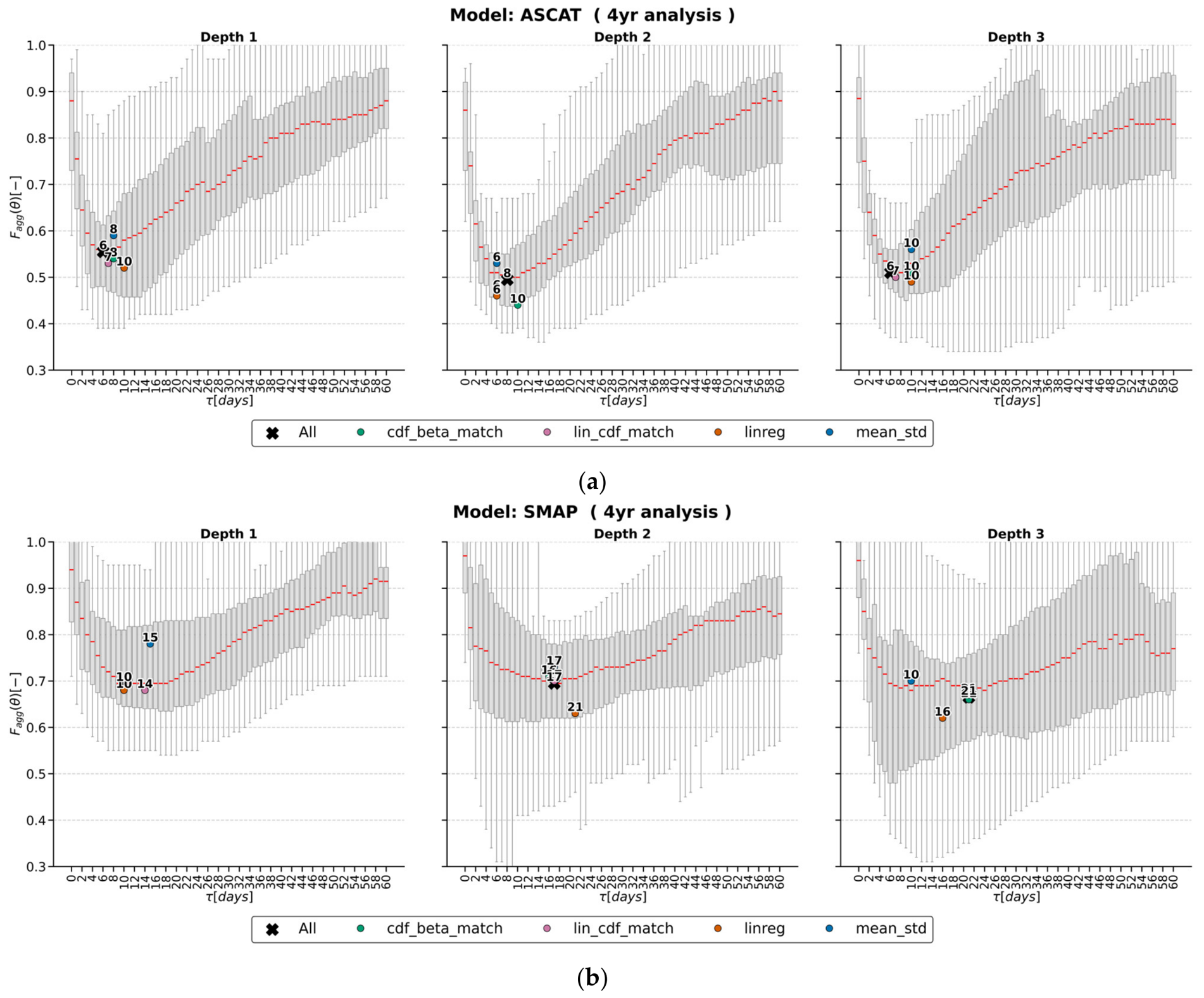
As mentioned in the main manuscript, this appendix presents the evaluation results obtained when extending the analysis over the full four-year study period (July 2021–July 2025). Figure A3 illustrates the sensitivity of the multi-objective function (Fagg) to the SWI time length (τ) for both ASCAT and SMAP products over this extended timeframe. Furthermore, Figure A4 details the Fagg performances across the nine monitoring stations, comparing the application of a locally optimized τ versus a fixed optimal τ. These extended results allow for a direct comparison with the two-year baseline analyses presented in the main text (Figure 4 and Figure 5, respectively).
Figure A3. Sensitivity of the multi-objective function Fagg to the SWI time length τ for the ASCAT product (a) and for the SMAP product (b), evaluated at the three different aggregation depths. Each boxplot represents the distribution of Fagg (9 × 4 = 36 values) across all nine stations and four tested rescaling methods (the min_max stretching method was excluded due to its systematically lower performance). In red the corresponding median boxes represent the interquartile range (IQR) and whiskers extend to 1.5 × IQR. The coloured markers highlight the optimal τ (i.e., yielding the minimum median Fagg) achieved by each specific rescaling technique, while the black cross represents the overall optimum when aggregating all rescaling methods. The results are obtained for the four-year period (July 2021–July 2025).
Remotesensing 18 02903 g0a3
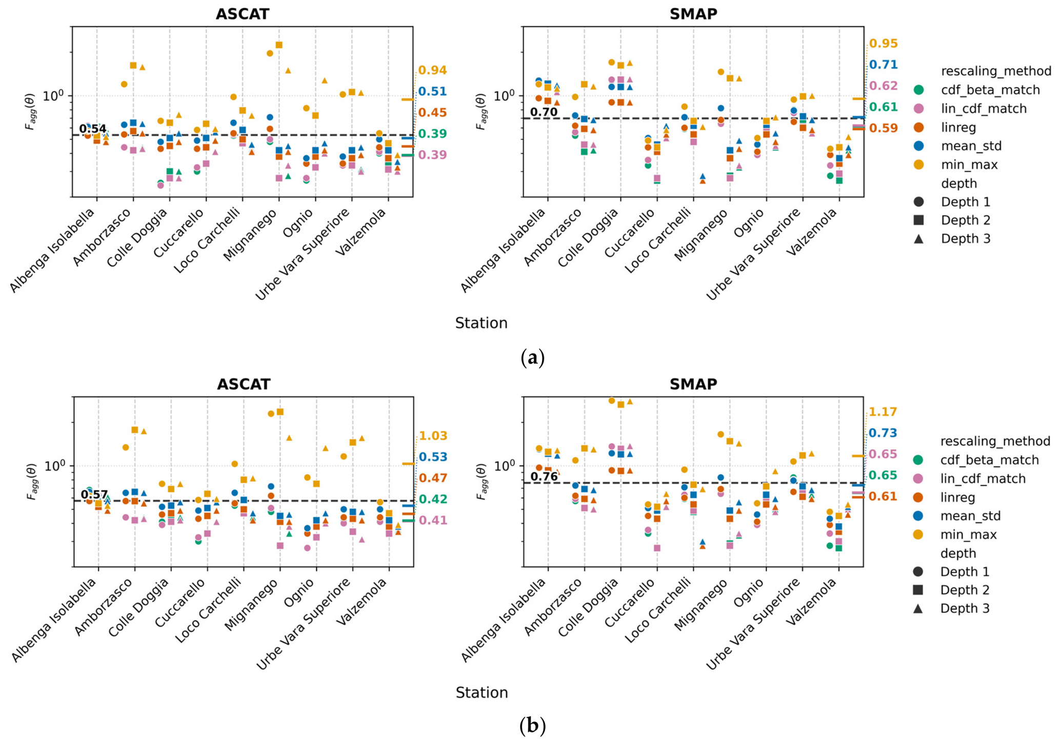
Figure A4. Scatterplots of the multi-objective function Fagg evaluated across the nine monitoring stations. Panel (a) presents the results for satellite-based (ASCAT, SMAP) products. The temporal exponential filter was applied using a locally optimized characteristic time length (τ) identified for each unique combination of rescaling method, soil depth, and station. Conversely, panel (b) uses a fixed optimal (τ = 7 days for ASCAT and τ = 16 days for SMAP). Marker colours differentiate the applied rescaling methods, while marker shapes denote the corresponding soil depth layer. The y-axis is presented on a logarithmic scale. The horizontal black dashed line (with the value on the left) indicates the overall mean Fagg for that specific product, whereas the coloured numerical values on the right y-axis report the specific mean performance achieved by each individual rescaling method. The results are obtained for the four-year period (July 2021–July 2025).
Remotesensing 18 02903 g0a4

References

  1. Scipal, K.; Scheffler, C.; Wagner, W. Soil Moisture-Runoff Relation at the Catchment Scale as Observed with Coarse Resolution Microwave Remote Sensing. Hydrol. Earth Syst. Sci. 2005, 9, 173–183. [Google Scholar] [CrossRef] [Scilit]
  2. Alfieri, L.; Avanzi, F.; Delogu, F.; Gabellani, S.; Bruno, G.; Campo, L.; Libertino, A.; Massari, C.; Tarpanelli, A.; Rains, D.; et al. High-Resolution Satellite Products Improve Hydrological Modeling in Northern Italy. Hydrol. Earth Syst. Sci. 2022, 26, 3921–3939. [Google Scholar] [CrossRef] [Scilit]
  3. Peng, J.; Albergel, C.; Balenzano, A.; Brocca, L.; Cartus, O.; Cosh, M.H.; Crow, W.T.; Dabrowska-Zielinska, K.; Dadson, S.; Davidson, M.W.J.; et al. A Roadmap for High-Resolution Satellite Soil Moisture Applications—Confronting Product Characteristics with User Requirements. Remote Sens. Environ. 2021, 252, 112162. [Google Scholar] [CrossRef] [Scilit]
  4. Dorigo, W.; Wagner, W.; Albergel, C.; Albrecht, F.; Balsamo, G.; Brocca, L.; Chung, D.; Ertl, M.; Forkel, M.; Gruber, A.; et al. ESA CCI Soil Moisture for Improved Earth System Understanding: State-of-the Art and Future Directions. Remote Sens. Environ. 2017, 203, 185–215. [Google Scholar] [CrossRef] [Scilit]
  5. Brocca, L.; Melone, F.; Moramarco, T.; Wagner, W.; Naeimi, V.; Bartalis, Z.; Hasenauer, S. Potential of ASCAT Soil Moisture Product to Improve Runoff Prediction. In Proceedings of the Symposium Earth Observation and Water Cycle Science, Frascati, Italy, 18–20 November 2009; European Space Agency (ESA): Noordwijk, The Netherlands, 2009; Volume 674, p. 15. [Google Scholar]
  6. Gruber, A.; Su, C.-H.; Zwieback, S.; Crow, W.; Dorigo, W.; Wagner, W. Recent Advances in (Soil Moisture) Triple Collocation Analysis. Int. J. Appl. Earth Obs. Geoinf. 2016, 45, 200–211. [Google Scholar] [CrossRef] [Scilit]
  7. Yi, C.; Li, X.; Zeng, J.; Fan, L.; Xie, Z.; Gao, L.; Xing, Z.; Ma, H.; Boudah, A.; Zhou, H.; et al. Assessment of Five SMAP Soil Moisture Products Using ISMN Ground-Based Measurements over Varied Environmental Conditions. J. Hydrol. 2023, 619, 129325. [Google Scholar] [CrossRef] [Scilit]
  8. Al-Yaari, A.; Wigneron, J.-P.; Dorigo, W.; Colliander, A.; Pellarin, T.; Hahn, S.; Mialon, A.; Richaume, P.; Fernandez-Moran, R.; Fan, L.; et al. Assessment and Inter-Comparison of Recently Developed/Reprocessed Microwave Satellite Soil Moisture Products Using ISMN Ground-Based Measurements. Remote Sens. Environ. 2019, 224, 289–303. [Google Scholar] [CrossRef] [Scilit]
  9. Feng, S.; Huang, X.; Zhao, S.; Qin, Z.; Fan, J.; Zhao, S. Evaluation of Several Satellite-Based Soil Moisture Products in the Continental US. Sensors 2022, 22, 9977. [Google Scholar] [CrossRef] [Scilit] [PubMed]
  10. ONeill, P.; Chan, S.; Njoku, E.; Jackson, T.; Bindlish, R.; Chaubell, J.; Colliander, A. SMAP Enhanced L2 Radiometer Half-Orbit 9 Km EASE-Grid Soil Moisture, Version 6; NASA NSIDC DAAC: Boulder, CO, USA, 2023. [CrossRef]
  11. Chan, S.K.; Bindlish, R.; O’Neill, P.; Jackson, T.; Njoku, E.; Dunbar, S.; Chaubell, J.; Piepmeier, J.; Yueh, S.; Entekhabi, D.; et al. Development and Assessment of the SMAP Enhanced Passive Soil Moisture Product. Remote Sens. Environ. 2018, 204, 931–941. [Google Scholar] [CrossRef] [Scilit] [PubMed]
  12. Wagner, W.; Hahn, S.; Kidd, R.; Melzer, T.; Bartalis, Z.; Hasenauer, S.; Figa-Saldana, J.; de Rosnay, P.; Jann, A.; Schneider, S.; et al. The ASCAT Soil Moisture Product: A Review of Its Specifications, Validation Results, and Emerging Applications. Meteorol. Z. 2013, 22, 5–33. [Google Scholar] [CrossRef] [Scilit]
  13. Balsamo, G.; Beljaars, A.; Scipal, K.; Viterbo, P.; van den Hurk, B.; Hirschi, M.; Betts, A.K. A Revised Hydrology for the ECMWF Model: Verification from Field Site to Terrestrial Water Storage and Impact in the Integrated Forecast System. J. Hydrometeorol. 2009, 10, 623–643. [Google Scholar] [CrossRef] [Scilit]
  14. Silvestro, F.; Gabellani, S.; Delogu, F.; Rudari, R.; Boni, G. Exploiting Remote Sensing Land Surface Temperature in Distributed Hydrological Modelling: The Example of the Continuum Model. Hydrol. Earth Syst. Sci. 2013, 17, 39–62. [Google Scholar] [CrossRef] [Scilit]
  15. Gruber, A.; De Lannoy, G.; Albergel, C.; Al-Yaari, A.; Brocca, L.; Calvet, J.-C.; Colliander, A.; Cosh, M.; Crow, W.; Dorigo, W.; et al. Validation Practices for Satellite Soil Moisture Retrievals: What Are (the) Errors? Remote Sens. Environ. 2020, 244, 111806. [Google Scholar] [CrossRef] [Scilit]
  16. Parinussa, R.M.; Meesters, A.G.C.A.; Liu, Y.Y.; Dorigo, W.; Wagner, W.; de Jeu, R.A.M. Error Estimates for Near-Real-Time Satellite Soil Moisture as Derived From the Land Parameter Retrieval Model. IEEE Geosci. Remote Sens. Lett. 2011, 8, 779–783. [Google Scholar] [CrossRef] [Scilit]
  17. de Nijs, A.H.A.; Parinussa, R.M.; de Jeu, R.A.M.; Schellekens, J.; Holmes, T.R.H. A Methodology to Determine Radio-Frequency Interference in AMSR2 Observations. IEEE Trans. Geosci. Remote Sens. 2015, 53, 5148–5159. [Google Scholar] [CrossRef] [Scilit]
  18. Wanders, N.; Karssenberg, D.; de Roo, A.; de Jong, S.M.; Bierkens, M.F.P. The Suitability of Remotely Sensed Soil Moisture for Improving Operational Flood Forecasting. Hydrol. Earth Syst. Sci. 2014, 18, 2343–2357. [Google Scholar] [CrossRef] [Scilit]
  19. Kwon, Y.; Liu, P.-W.; Navari, M.; Bindlish, R.; Kemp, E.M.; Wegiel, J.W.; Jalilvand, E.; Kumar, S.V. Development of Low Latency, High Resolution SMAP Soil Moisture Retrievals in Support of near-Real-Time Applications. Front. Earth Sci. 2026, 14, 1854083. [Google Scholar] [CrossRef] [Scilit]
  20. AllertaLiguria—Protezione Civile: Chi Fa Cosa. Available online: https://allertaliguria.regione.liguria.it/protezione_civile.php (accessed on 6 November 2025).
  21. Rebora, N.; Molini, L.; Casella, E.; Comellas, A.; Fiori, E.; Pignone, F.; Siccardi, F.; Silvestro, F.; Tanelli, S.; Parodi, A. Extreme Rainfall in the Mediterranean: What Can We Learn from Observations? J. Hydrometeorol. 2013, 14, 906–922. [Google Scholar] [CrossRef] [Scilit]
  22. Silvestro, F.; Parodi, A.; Campo, L.; Ferraris, L. Analysis of the Streamflow Extremes and Long-Term Water Balance in the Liguria Region of Italy Using a Cloud-Permitting Grid Spacing Reanalysis Dataset. Hydrol. Earth Syst. Sci. 2018, 22, 5403–5426. [Google Scholar] [CrossRef] [Scilit]
  23. Giannoni, F.; Roth, G.; Rudari, R. A Procedure for Drainage Network Identification from Geomorphology and Its Application to the Prediction of the Hydrologic Response. Adv. Water Resour. 2005, 28, 567–581. [Google Scholar] [CrossRef] [Scilit]
  24. Gabellani, S.; Silvestro, F.; Rudari, R.; Boni, G. General Calibration Methodology for a Combined Horton-SCS Infiltration Scheme in Flash Flood Modeling. Nat. Hazards Earth Syst. Sci. 2008, 8, 1317–1327. [Google Scholar] [CrossRef] [Scilit]
  25. Poggio, L.; de Sousa, L.M.; Batjes, N.H.; Heuvelink, G.B.M.; Kempen, B.; Ribeiro, E.; Rossiter, D. SoilGrids 2.0: Producing Soil Information for the Globe with Quantified Spatial Uncertainty. SOIL 2021, 7, 217–240. [Google Scholar] [CrossRef] [Scilit]
  26. Davolio, S.; Silvestro, F.; Gastaldo, T. Impact of Rainfall Assimilation on High-Resolution Hydrometeorological Forecasts over Liguria, Italy. J. Hydrometeorol. 2017, 18, 2659–2680. [Google Scholar] [CrossRef] [Scilit]
  27. Albergel, C.; Dutra, E.; Munier, S.; Calvet, J.-C.; Munoz-Sabater, J.; de Rosnay, P.; Balsamo, G. ERA-5 and ERA-Interim Driven ISBA Land Surface Model Simulations: Which One Performs Better? Hydrol. Earth Syst. Sci. 2018, 22, 3515–3532. [Google Scholar] [CrossRef] [Scilit]
  28. de Rosnay, P.; Drusch, M.; Vasiljevic, D.; Balsamo, G.; Albergel, C.; Isaksen, L. A Simplified Extended Kalman Filter for the Global Operational Soil Moisture Analysis at ECMWF. Q. J. R. Meteorol. Soc. 2013, 139, 1199–1213. [Google Scholar] [CrossRef] [Scilit]
  29. Fairbairn, D.; de Rosnay, P. Algorithm Theoretical Baseline Document (ATBD) H26; EUMETSAT: Darmstadt, Germany, 2021. [Google Scholar]
  30. Fairbairn, D.; de Rosnay, P. Algorithm Theoretical Baseline Document (ATBD) H141 and H142; EUMETSAT: Darmstadt, Germany, 2020. [Google Scholar]
  31. Entekhabi, D.; Njoku, E.G.; O’Neill, P.E.; Kellogg, K.H.; Crow, W.T.; Edelstein, W.N.; Entin, J.K.; Goodman, S.D.; Jackson, T.J.; Johnson, J.; et al. The Soil Moisture Active Passive (SMAP) Mission. Proc. IEEE 2010, 98, 704–716. [Google Scholar] [CrossRef] [Scilit]
  32. Colliander, A.; Jackson, T.J.; Bindlish, R.; Chan, S.; Das, N.; Kim, S.B.; Cosh, M.H.; Dunbar, R.S.; Dang, L.; Pashaian, L.; et al. Validation of SMAP Surface Soil Moisture Products with Core Validation Sites. Remote Sens. Environ. 2017, 191, 215–231. [Google Scholar] [CrossRef] [Scilit]
  33. Chan, S. Enhanced Level 2 Passive Soil Moisture Product Specification Document; JPL D-56291; Jet Propulsion Laboratory California Institute of Technology: Pasadena, CA, USA, 2019. [Google Scholar]
  34. Poe, G.A. Optimum Interpolation of Imaging Microwave Radiometer Data. IEEE Trans. Geosci. Remote Sens. 1990, 28, 800–810. [Google Scholar] [CrossRef] [Scilit]
  35. Chaubell, J.; Chan, S.; Dunbar, R.; Peng, J.; Yueh, S. SMAP Enhanced L1C Radiometer Half-Orbit 9 Km EASE-Grid Brightness Temperatures; NASA National Snow and Ice Data Center Distributed Active Archive Center: Boulder, CO, USA, 2018.
  36. Hahn, S. Algorithm Theoretical Baseline Document (ATBD) Surface Soil Moisture ASCAT NRT Orbit (H101, H102, H16, H103, H106, H107); EUMETSAT: Darmstadt, Germany, 2016. [Google Scholar]
  37. Wagner, W.; Lemoine, G.; Rott, H. A Method for Estimating Soil Moisture from ERS Scatterometer and Soil Data. Remote Sens. Environ. 1999, 70, 191–207. [Google Scholar] [CrossRef] [Scilit]
  38. New Global Hydrography Derived From Spaceborne Elevation Data—Lehner—2008—Eos, Transactions American Geophysical Union—Wiley Online Library; Available online: https://agupubs.onlinelibrary.wiley.com/doi/10.1029/2008EO100001 (accessed on 30 July 2026).
  39. ISPRA Copertura Del Suolo 2023: Uso, Copertura e Consumo di Suolo. Available online: https://groupware.sinanet.isprambiente.it/uso-copertura-e-consumo-di-suolo/library/copertura-del-suolo/carta-di-copertura-del-suolo/copertura-del-suolo-2023 (accessed on 4 April 2026).
  40. Brocca, L.; Melone, F.; Moramarco, T.; Wagner, W.; Albergel, C. Scaling and Filtering Approaches for the Use of Satellite Soil Moisture Observations. Remote Sens. Energy Fluxes Soil Moisture Content 2013, 1, 411–426. [Google Scholar] [CrossRef] [Scilit]
  41. Scipal, K.; Drusch, M.; Wagner, W. Assimilation of a ERS Scatterometer Derived Soil Moisture Index in the ECMWF Numerical Weather Prediction System. Adv. Water Resour. 2008, 31, 1101–1112. [Google Scholar] [CrossRef] [Scilit]
  42. Jackson, T.J.; Cosh, M.H.; Bindlish, R.; Starks, P.J.; Bosch, D.D.; Seyfried, M.; Goodrich, D.C.; Moran, M.S.; Du, J. Validation of Advanced Microwave Scanning Radiometer Soil Moisture Products. IEEE Trans. Geosci. Remote Sens. 2010, 48, 4256–4272. [Google Scholar] [CrossRef] [Scilit]
  43. Lacava, T.; Brocca, L.; Calice, G.; Melone, F.; Moramarco, T.; Pergola, N.; Tramutoli, V. Soil Moisture Variations Monitoring by AMSU-Based Soil Wetness Indices: A Long-Term Inter-Comparison with Ground Measurements. Remote Sens. Environ. 2010, 114, 2317–2325. [Google Scholar] [CrossRef] [Scilit]
  44. Madsen, H. Automatic Calibration of a Conceptual Rainfall–Runoff Model Using Multiple Objectives. J. Hydrol. 2000, 235, 276–288. [Google Scholar] [CrossRef] [Scilit]
  45. Madsen, H.; Wilson, G.; Ammentorp, H.C. Comparison of Different Automated Strategies for Calibration of Rainfall-Runoff Models. J. Hydrol. 2002, 261, 48–59. [Google Scholar] [CrossRef] [Scilit]
  46. Brocca, L.; Melone, F.; Moramarco, T.; Wagner, W.; Hasenauer, S. ASCAT Soil Wetness Index Validation through in Situ and Modeled Soil Moisture Data in Central Italy. Remote Sens. Environ. 2010, 114, 2745–2755. [Google Scholar] [CrossRef] [Scilit]
  47. Draper, C.S.; Walker, J.P.; Steinle, P.J.; de Jeu, R.A.M.; Holmes, T.R.H. An Evaluation of AMSR–E Derived Soil Moisture over Australia. Remote Sens. Environ. 2009, 113, 703–710. [Google Scholar] [CrossRef] [Scilit]
  48. Taylor, K.E. Summarizing Multiple Aspects of Model Performance in a Single Diagram. J. Geophys. Res. Atmos. 2001, 106, 7183–7192. [Google Scholar] [CrossRef] [Scilit]
  49. Entekhabi, D.; Reichle, R.H.; Koster, R.D.; Crow, W.T. Performance Metrics for Soil Moisture Retrievals and Application Requirements. J. Hydrometeorol. 2010, 11, 832–840. [Google Scholar] [CrossRef] [Scilit]
  50. Pascale, S.; Ragone, F. Widespread Multi-Year Droughts in Italy: Identification and Causes of Development. Int. J. Climatol. 2025, 45, e8827. [Google Scholar] [CrossRef] [Scilit]
  51. Xing, Z.; Fan, L.; Zhao, L.; De Lannoy, G.; Frappart, F.; Peng, J.; Li, X.; Zeng, J.; Al-Yaari, A.; Yang, K.; et al. A First Assessment of Satellite and Reanalysis Estimates of Surface and Root-Zone Soil Moisture over the Permafrost Region of Qinghai-Tibet Plateau. Remote Sens. Environ. 2021, 265, 112666. [Google Scholar] [CrossRef] [Scilit]
  52. Beck, H.E.; Pan, M.; Miralles, D.G.; Reichle, R.H.; Dorigo, W.A.; Hahn, S.; Sheffield, J.; Karthikeyan, L.; Balsamo, G.; Parinussa, R.M.; et al. Evaluation of 18 Satellite- and Model-Based Soil Moisture Products Using in Situ Measurements from 826 Sensors. Hydrol. Earth Syst. Sci. 2021, 25, 17–40. [Google Scholar] [CrossRef] [Scilit]
  53. Massari, C.; Brocca, L.; Barbetta, S.; Papathanasiou, C.; Mimikou, M.; Moramarco, T. Using Globally Available Soil Moisture Indicators for Flood Modelling in Mediterranean Catchments. Hydrol. Earth Syst. Sci. 2014, 18, 839–853. [Google Scholar] [CrossRef] [Scilit]
  54. Mohite, J.; Sawant, S.; Pandit, A.; Pappula, S. Spatial Downscaling of Smap Soil Moisture Using the Modis and Srtm Observations. Int. Arch. Photogramm. Remote Sens. Spat. Inf. Sci. 2022, XLIII-B3-2022, 933–938. [Google Scholar] [CrossRef] [Scilit]
  55. Peng, J.; Loew, A.; Merlin, O.; Verhoest, N.E.C. A Review of Spatial Downscaling of Satellite Remotely Sensed Soil Moisture. Rev. Geophys. 2017, 55, 341–366. [Google Scholar] [CrossRef] [Scilit]
  56. Afshar, M.H.; Yilmaz, M.T.; Crow, W.T. Impact of Rescaling Approaches in Simple Fusion of Soil Moisture Products. Water Resour. Res. 2019, 55, 7804–7825. [Google Scholar] [CrossRef] [Scilit]
  57. Yilmaz, M.T.; Crow, W.T.; Ryu, D. Impact of Model Relative Accuracy in Framework of Rescaling Observations in Hydrological Data Assimilation Studies. J. Hydrometeorol. 2016, 17, 2245–2257. [Google Scholar] [CrossRef] [Scilit]
  58. Stroud, P. A Recursive Exponential Filter for Time-Sensitive Data; Los Alamos National Laboratory: Los Alamos, NM, USA, 1999.
  59. Albergel, C.; Rüdiger, C.; Carrer, D.; Calvet, J.-C.; Fritz, N.; Naeimi, V.; Bartalis, Z.; Hasenauer, S. An Evaluation of ASCAT Surface Soil Moisture Products with In-Situ Observations in Southwestern France. Hydrol. Earth Syst. Sci. 2009, 13, 115–124. [Google Scholar] [CrossRef] [Scilit]
  60. Albergel, C.; Rüdiger, C.; Pellarin, T.; Calvet, J.-C.; Fritz, N.; Froissard, F.; Suquia, D.; Petitpa, A.; Piguet, B.; Martin, E. From Near-Surface to Root-Zone Soil Moisture Using an Exponential Filter: An Assessment of the Method Based on in-Situ Observations and Model Simulations. Hydrol. Earth Syst. Sci. 2008, 12, 1323–1337. [Google Scholar] [CrossRef] [Scilit]
  61. Laiolo, P.; Gabellani, S.; Campo, L.; Cenci, L.; Silvestro, F.; Delogu, F.; Boni, G.; Rudari, R.; Puca, S.; Pisani, A.R. Assimilation of Remote Sensing Observations into a Continuous Distributed Hydrological Model: Impacts on the Hydrologic Cycle. In Proceedings of the 2015 IEEE International Geoscience and Remote Sensing Symposium (IGARSS), Milan, Italy, 26–31 July 2015; pp. 1308–1311. [Google Scholar]
  62. Ortenzi, S.; Cencetti, C.; Mincu, F.-I.; Neculau, G.; Chendeş, V.; Ciabatta, L.; Massari, C.; Di Matteo, L. Comparing Satellite Soil Moisture Products Using In Situ Observations over an Instrumented Experimental Basin in Romania. Remote Sens. 2024, 16, 3283. [Google Scholar] [CrossRef] [Scilit]
  63. Hjerdt, K.N.; McDonnell, J.J.; Seibert, J.; Rodhe, A. A New Topographic Index to Quantify Downslope Controls on Local Drainage. Water Resour. Res. 2004, 40, W05602. [Google Scholar] [CrossRef] [Scilit]
Figure 1. Ligurian Region boundaries (solid black line), provincial borders (dotted black line) and contour lines. The nine monitoring stations equipped with FDR sensors used in this study are shown in red. The basemap is derived from OpenStreetMap data (https://www.openstreetmap.org/).
Remotesensing 18 02903 g001
Figure 2. Volumetric Water Content (VWC [m3 m−3]) time series measured at the Urbe Vara Superiore station at the three different aggregation depths. The lower panel shows the daily precipitation hyetographs recorded at the same station (mm/24 h).
Remotesensing 18 02903 g002
Figure 3. A schematic overview of the methodology adopted in this analysis.
Remotesensing 18 02903 g003
Figure 4. Sensitivity of the multi-objective function Fagg to the SWI time length τ for the ASCAT product (a) and for the SMAP product (b), evaluated at the three different aggregation depths. Each boxplot represents the distribution of Fagg (9 × 4 = 36 values) across all nine stations and four tested rescaling methods (the min_max stretching method was excluded due to its systematically lower performance). In red the corresponding median, boxes represent the interquartile range (IQR) and whiskers extend to 1.5 × IQR. The coloured markers highlight the optimal τ (i.e., yielding the minimum median Fagg) achieved by each specific rescaling technique, while the black cross represents the overall optimum when aggregating all rescaling methods. The results are obtained for the two-year period (July 2023–July 2025).
Remotesensing 18 02903 g004
Figure 5. Scatterplots of the multi-objective function Fagg evaluated across the nine monitoring stations. Panel (a) presents the results for satellite-based (ASCAT, SMAP) products. The temporal exponential filter was applied using a locally optimized characteristic time length (τ) identified for each unique combination of rescaling method, soil depth, and station. Conversely, panel (b) uses a fixed optimal (τ = 8 days for ASCAT and τ = 25 days for SMAP). Marker colours differentiate the applied rescaling methods, while marker shapes denote the corresponding soil depth layer. The y-axis is presented on a logarithmic scale. The horizontal black dashed line (with the value on the left) indicates the overall mean Fagg for that specific product, whereas the coloured numerical values on the right y-axis report the specific mean performance achieved by each individual rescaling method. The results are obtained for the two-year period (July 2023–July 2025).
Remotesensing 18 02903 g005
Figure 6. Heatmaps summarizing the Fagg across the evaluated stations and SM products. Panel (a) displays results for the two-year period (July 2023–July 2025), whereas panel (b) presents the extended four-year analysis. For every combination of monitoring station (y-axis), rescaled SM product (x-axis), and reference depth (columns), the cells display the minimum achieved value of the multi-objective function, Fagg systematically evaluating all possible combinations of rescaling methods and, exclusively for satellite-derived products, all tested SWI characteristic time lengths (τ). Blue shades indicate lower Fagg values (corresponding to a stronger agreement with in situ VWC observations), while warmer colours denote poorer performance.
Remotesensing 18 02903 g006
Figure 7. Taylor diagrams for all analyzed stations and soil moisture products, categorized by the five tested rescaling methods. The purple star (“Ref”) represents the in situ ground reference. The solid black arc indicates a normalized standard deviation of 1.0, while dashed red semi-circles denote the normalized ubRMSE isolines (0.5, 1.0, and 1.5). The plotted data points encompass results from both the two-year and four-year analysis periods. Results with negative Pearson correlation (R < 0) or a negative Nash–Sutcliffe Efficiency (NSE < 0) were excluded from this visualization. For a detailed explanation of the diagram metrics and coordinate system, please refer to Section 2.4.5.
Remotesensing 18 02903 g007
Figure 8. Time series comparison at the Cuccarello station (Depth 1) between the in situ reference observations and four rescaled soil moisture products, displayed in separate subpanels. From top to bottom: (1) Continuum, (2) ECMWF 0–7 cm, (3) ASCAT SWI (τ = 5 days), and (4) SMAP SWI (τ = 7 days) Both the rescaled and reference time series are expressed as Volumetric Water Content (VWC) [m3 m−3]. For illustrative purposes, the τ values were fixed according to the optimal results obtained via the CDF Beta Matching technique.
Remotesensing 18 02903 g008
Table 1. List of datasets including the ground measurement used as reference sample and the processed soil moisture products.
SourceTypeInstrument/ModelProductSpatial ResolutionTemporal ResolutionData AvailabilitySM-Output Units
OMIRLPoint
Measurement
FDR-Sensor-In situ1 h2021-nowSMVWC [m3 m−3]
ASCATSatelliteC-band VV-Radar H16~12.5 km~1 day2007-nowSSMS [m3 m−3]
SMAPSatelliteL-band RadiometerL2SMP_E~9 km~0.5 day2015-nowSSMVWC [m3 m−3]
HMC ModelledHydrological Model-~200 m1 h2006-nowRZ SMS [m3 m−3]
HTESSELModelledLand Surface ModelH142; H26~10 km1 day1992-nowRZ
Liquid SWI
S [m3 m−3]
Table 2. Local soil properties for the evaluated stations. Mean Column Porosity (0–30 cm) is extracted from SoilGrids data at the station coordinates by averaging the values from the first three depth layers (0–5 cm, 5–15 cm, and 15–30 cm). Soil type is also derived from the same SoilGrids dataset. The maximum storage volume Vmax (in equivalent water depth) refer to the overlaying pixel of HMC. The estimated root-zone (RZ) depth is calculated as the ratio of Vmax to porosity.
StationCoordinates
(°N, °E)
Elevation [m a.s.l.]Soil TypePorosity
[-]
Vmax
[mm]
RZ Depth
[mm]
Amborzasco44.51447, 9.45496908Compact Clay0.59160270
Colle D’Oggia43.98131, 7.866671163Draining Porous0.55170310
Cuccarello44.34967, 9.69908835Draining Porous0.61137220
Albenga Isolabella44.06875, 8.1795636----
Loco Carchelli44.55421, 9.28421600Draining Porous0.60106180
Mignanego44.54028, 8.93816270Compact Clay0.52157300
Ognio44.44372, 9.16994490Compact Clay0.56197350
Urbe—Vara Sup.44.46953, 8.62739810Draining Porous0.55137250
Valzemola44.36959, 8.19105480Compact Clay0.48126260
Table 3. Comparison of topographic and land cover characteristics at two spatial resolutions (300 m for the HMC model and 12.5 km for satellite/ECMWF products). Elevation ranges are reported in metres above sea level (m a.s.l.) derived from the hydrologically conditioned DEM of [38], while land cover fractions are expressed as percentages (%). Land cover classes are derived from [39]. * Other: minor land cover classes, including consolidated surfaces, unconsolidated surfaces, shrub vegetation, permanent water bodies, and wetlands.
StationElev. Range [m a.s.l.]Artificial Impervious [%]Forests (Conifers + Broadleaf) [%]Grasslands [%]* Other [%]
300 m buffer
Amborzasco789–9321143460
Colle D’Oggia897–1257444530
Cuccarello736–942179210
Albenga-Isolabella14–37303643
Loco Carchelli577–6741260200
Mignanego239–3961668150
Ognio339–63397795
Urbe Vara S.742–8692150290
Valzemola415–5041535490
12.5 km buffer
Amborzasco134–1769282133
Colle D’Oggia38–2090382114
Cuccarello106–1592383113
Albenga-Isolabella0–13421067149
Loco Carchelli249–1600286102
Mignanego15–1172774173
Ognio0–1401681103
Urbe Vara S.0–1274569188
Valzemola296–1214577171
Table 4. Performance metrics for the evaluated soil moisture products across three depths, using the linear CDF matching and the linear rescaling method. Values are expressed as the median ± standard deviation calculated across the stations.
Model τ lin_cdf_matchmean_std
ubRMSE [m3 m−3]CCNSEFagg ubRMSE
[m3 m−3]
CCNSEFagg
Depth 1
Continuum-0.020 ± 0.0070.860 ± 0.0480.730 ± 0.0960.230 ± 0.1070.023 ± 0.0080.860 ± 0.0360.720 ± 0.0700.240 ± 0.078
ECMWF
0–7 cm
-0.029 ± 0.0060.860 ± 0.0350.710 ± 0.0700.250 ± 0.0800.030 ± 0.0070.860 ± 0.0360.710 ± 0.0670.250 ± 0.075
ASCATτopt0.032 ± 0.0090.780 ± 0.0590.570 ± 0.1150.410 ± 0.1290.037 ± 0.0080.740 ± 0.0530.490 ± 0.1060.500 ± 0.120
ASCAT8 days0.034 ± 0.0090.780 ± 0.0520.570 ± 0.1070.410 ± 0.1190.038 ± 0.0090.730 ± 0.0510.470 ± 0.1010.520 ± 0.113
SMAPτopt0.035 ± 0.0170.700 ± 0.1590.390 ± 0.3240.600 ± 0.3620.040 ± 0.0150.640 ± 0.1300.280 ± 0.2640.730 ± 0.292
SMAP25 days0.035 ± 0.0180.690 ± 0.1690.370 ± 0.3480.630 ± 0.3880.040 ± 0.0150.640 ± 0.1380.280 ± 0.2780.730 ± 0.311
Depth 2
Continuum-0.015 ± 0.0090.885 ± 0.0490.760 ± 0.0990.190 ± 0.1090.019 ± 0.0100.865 ± 0.0350.735 ± 0.0690.225 ± 0.077
ECMWF
0–28 cm
-0.022 ± 0.0060.890 ± 0.0380.770 ± 0.0730.180 ± 0.0820.022 ± 0.0070.890 ± 0.0320.780 ± 0.0650.170 ± 0.073
ASCATτopt0.027 ± 0.0110.815 ± 0.0470.635 ± 0.0970.335 ± 0.1060.033 ± 0.0100.740 ± 0.0400.470 ± 0.0760.510 ± 0.086
ASCAT8 days0.029 ± 0.0110.795 ± 0.0440.595 ± 0.0890.380 ± 0.1000.033 ± 0.0100.735 ± 0.0380.470 ± 0.0760.520 ± 0.086
SMAPτopt0.035 ± 0.0190.730 ± 0.1720.460 ± 0.3390.525 ± 0.3810.038 ± 0.0170.670 ± 0.1360.340 ± 0.2700.660 ± 0.301
SMAP25 days0.036 ± 0.0190.720 ± 0.1770.450 ± 0.3520.540 ± 0.3940.039 ± 0.0170.675 ± 0.1370.340 ± 0.2720.660 ± 0.305
Depth 3
Continuum-0.018 ± 0.0140.910 ± 0.0690.810 ± 0.1350.130 ± 0.1510.020 ± 0.0110.890 ± 0.0530.770 ± 0.1070.180 ± 0.119
ASCATτopt0.030 ± 0.0100.790 ± 0.0460.570 ± 0.0890.400 ± 0.1010.035 ± 0.0090.720 ± 0.0420.440 ± 0.0860.550 ± 0.096
ASCAT8 days0.031 ± 0.0100.780 ± 0.0380.570 ± 0.0720.410 ± 0.0810.035 ± 0.0090.720 ± 0.0360.430 ± 0.0780.560 ± 0.088
SMAPτopt0.034 ± 0.0160.740 ± 0.1590.470 ± 0.3090.510 ± 0.3480.037 ± 0.0150.660 ± 0.1300.320 ± 0.2600.680 ± 0.291
SMAP25 days0.034 ± 0.0170.730 ± 0.1690.470 ± 0.3320.520 ± 0.3730.037 ± 0.0150.660 ± 0.1270.320 ± 0.2530.680 ± 0.284
Table 5. Performance metrics’ function on Cuccarello station at Depth 1 with rescaled (1) Continuum, (2) ECMWF at 0–7 cm (3) ASCAT SWI (τ = 5 days) and SMAP SWI (τ = 7 days).
Rescaling Methodτ [Days]CC [-]ubRMSE [m3 m−3]NSE [-]Pbias [%]Fagg(θ) [−]
Continuum
cdf_beta_match-0.880.0180.760.00.19
linreg-0.860.0190.740.00.22
min_max-0.860.0210.61−3.90.34
mean_std-0.860.0200.720.00.24
ECMWF 0–7 cm
cdf_beta_match-0.810.0240.620.00.35
linreg-0.800.0230.650.00.33
min_max-0.800.0240.357.10.61
mean_std-0.800.0240.610.00.36
ASCAT
cdf_beta_match5 0.790.0250.580.00.39
linreg5 0.750.0260.560.00.43
min_max5 0.750.0280.12−8.20.84
mean_std5 0.750.0270.50.00.48
SMAP
cdf_beta_match7 0.700.0300.400.00.59
linreg7 0.680.0280.460.00.55
min_max7 0.680.0300.37−1.80.63
mean_std7 0.680.0310.350.00.65
Disclaimer/Publisher’s Note: The statements, opinions and data contained in all publications are solely those of the individual author(s) and contributor(s) and not of MDPI and/or the editor(s). MDPI and/or the editor(s) disclaim responsibility for any injury to people or property resulting from any ideas, methods, instructions or products referred to in the content.