Article

Process-Informed Satellite-Ground Fusion for Coastal Compound Humid-Heat and Photochemical Oxidant Early Warning

Graduate School of Informatics, Osaka Metropolitan University, Osaka 559-8531, Japan
*
Author to whom correspondence should be addressed.
Remote Sens. 2026, 18(17), 2874; https://doi.org/10.3390/rs18172874
Submission received: 30 June 2026 / Revised: 11 August 2026 / Accepted: 17 August 2026 / Published: 25 August 2026

Highlights

What are the main findings?
  • Previous-day MODIS improved probability quality and low-false-alarm warning allocation beyond a strong ground–ERA5–CAMS route; with the same 18 MODIS variables, it increased average precision over same-day MODIS by 0.0378 (95% CI: 0.0144–0.0603).
  • The MODIS increment was concentrated during high-heat issue times and in Osaka Bay and was reproduced in Temporal FLOW; matched spatial controls identified distance as the stable 24 h spatial backbone and wind as the complementary context.
What are the implications of the main findings?
  • Satellite value in early warning should be demonstrated through temporally matched source contrasts and validation-locked alert policies rather than inferred from generic multimodal inclusion.
  • Previous-day MODIS provides latency-aware thermal-memory information for coastal warning, with forecast-consistent and multi-bay confirmation as the next validation step.

Abstract

Coastal humid-heat and photochemical-oxidant episodes are commonly studied through concentration estimation, leaving it unclear whether satellite observations improve warning decisions under explicit false-alarm constraints. This study introduces CoAST-EWS Japan, a six-station, validation-locked hindcast benchmark across Osaka Bay and Tokyo Bay. Models were developed using June–July 2023 data, calibrated and thresholded on August 2023 predictions, and retrospectively evaluated on June–August 2025 station-hour observations. The strong non-satellite route combines recent ground history, ERA5 meteorology, CAMS composition, and static station geometry. Adding previous-day MODIS thermal context to an otherwise identical XGBoost route increased average precision from 0.3153 to 0.3429, reduced the Brier score from 0.05032 to 0.04874, and improved recall/F1 under a validation-locked budget of 0.5 false alarms per station-day (FPDs) from 0.1864/0.2511 to 0.2402/0.3042. Japan-local calendar-day intervals supported the improvements in Brier score, recall, and F1. In a dimension-matched comparison using the same 18 MODIS variables, previous-day context increased average precision over the same-day route by 0.0378 (95% CI: 0.0144–0.0603), demonstrating that the timing advantage was not attributable to a larger satellite feature set. The MODIS increment was strongest during high-heat issue times and in Osaka Bay, and its ranking value was reproduced by a 36 h Temporal FLOW model. Matched spatial controls identified distance-based coastal context as the most stable 24 h graph component, while wind-aligned information operated as a complementary route. These results establish latency-aware MODIS thermal context as a measurable decision input for neighborhood-scale coastal compound warning. Strict station-level localization, cross-bay transfer, and forecast-consistent deployment define the next validation frontier.

1. Introduction

Coastal cities are particularly susceptible to compound humid-heat and photochemical-oxidant episodes because thermal stress, atmospheric stagnation, solar radiation, precursor chemistry, boundary-layer evolution, and sea-breeze recirculation can reinforce one another over densely populated urban corridors. Concurrent heat and oxidant extremes create a warning problem that is distinct from either heat-stress assessment or ozone prediction alone: the relevant decision is not only how accurately an environmental variable can be reconstructed, but which station-hours should be prioritized before a future compound event occurs. This distinction is consequential in coastal environments, where event occurrence can depend on both local thermal conditions and spatially displaced oxidant observations [1,2].
Satellite-enhanced air-quality studies have substantially improved the spatial and temporal characterization of the ozone and related atmospheric composition. TROPOMI, MODIS, meteorological reanalysis, and other Earth-observation products have been combined with random forests, knowledge-informed neural networks, and multiscale fusion architectures to estimate surface ozone, retrieve spatially continuous pollutant fields, and improve prediction in data-sparse areas [3,4,5,6,7,8]. These studies establish that satellite observations can enrich concentration estimation, particularly by providing column composition, surface thermal state, and spatial context that are unavailable from sparse monitoring networks alone. Their principal outputs, however, remain continuous concentration fields or exposure estimates evaluated through measures such as R2, RMSE, MAE, and spatial reconstruction accuracy. Such metrics do not directly determine whether a satellite source improves alert allocation under a constrained false-alarm budget.
A parallel line of research has introduced graph-based and transport-aware architectures for multi-station air-quality prediction. Wind-aware dynamic graphs represent anisotropic pollutant transport, while multiscale graph attention and temporal encoders capture neighborhood dependence, long-range temporal structure, and cross-regional variability [9,10]. These methods provide an important architectural basis for spatially coupled warning models. Nevertheless, their graph structures are generally optimized for concentration forecasting or inference in monitored and unmonitored regions. They do not establish whether directional wind information improves a compound binary warning decision relative to simpler distance-based spatial context, nor do they evaluate that question under validation-locked alert policies.
Research on compound heat–ozone extremes addresses a different but complementary dimension of the problem. Observational and meteorology–chemistry studies have shown that high temperature, intense radiation, altered boundary-layer mixing, precursor redistribution, and nonlinear photochemistry jointly intensify urban ozone during heat extremes [1,2]. This literature provides the physical basis for combining thermal, meteorological, composition, and transport information. Its primary objectives are mechanism attribution, exposure characterization, and mitigation analysis rather than lead-specific station-hour warning. Consequently, the decision value of satellite observations has rarely been isolated from strong meteorological baselines within a compound-warning framework.
These three research streams leave a specific methodological gap. Existing studies do not directly quantify whether a temporally available satellite observation improves compound-warning decisions beyond recent ground conditions, meteorological reanalysis, and atmospheric-composition context. They also rarely distinguish satellite value from the value of reanalysis products, compare same-day and latency-safer satellite joins using matched variables, or lock alert thresholds before retrospective cross-year evaluation. As a result, the presence of satellite variables in a multimodal feature stack does not by itself establish that satellite observations improve the warning decision. A decision-oriented remote-sensing benchmark should therefore answer three questions: how much satellite observations add beyond a strong non-satellite baseline, under which environmental and availability conditions that increment appears, and whether the gain persists under fixed false-alarm constraints. Table 1 positions the present decision-oriented estimand relative to these three research streams.
Table 1 shows that the distinction lies not simply in the combination of additional sources, but in the evaluation target: the present study measures the incremental decision value of remotely sensed thermal context under a warning policy fixed before retrospective testing.
This study addresses these questions through CoAST-EWS Japan, a six-station hindcast benchmark spanning Osaka Bay and Tokyo Bay. Ground-observed wet-bulb globe temperature and photochemical-oxidant exceedances define lead-specific compound-warning labels, while ground history, ERA5 meteorology, CAMS composition, MODIS land-surface temperature, station geometry, and spatial graph context provide predictive information. Models are developed using June–July 2023 data, calibrated and thresholded using August 2023 predictions, and retrospectively evaluated on June–August 2025 station-hour observations. The principal satellite analysis compares an otherwise identical ground–ERA5–CAMS route with and without previous-day MODIS context. A dimension-matched experiment further compares same-day and previous-day versions of the same 18 MODIS variables, separating source timing from feature dimensionality. Temporal FLOW and matched graph controls test whether the satellite increment transfers across model families and whether spatial gains arise primarily from distance or directional wind context.
This study makes four contributions. First, it formulates coastal compound warning as a validation-locked rare-event decision problem, connecting probability quality to explicit false alarms per station-day rather than to an arbitrary classification threshold. Second, it provides direct evidence of satellite incremental value beyond a strong non-satellite baseline: previous-day MODIS improves probability quality and low-budget warning allocation, and its average-precision advantage over same-day MODIS remains positive in a dimension-matched comparison. Third, it identifies the conditions under which satellite thermal context is most informative, with the largest increments occurring during high-heat issue times and in Osaka Bay, while a 36 h Temporal FLOW model reproduces the ranking gain. Fourth, matched spatial controls show that distance-based coastal structure supplies the most stable 24 h graph contribution, whereas wind-aligned information is more appropriately used as complementary routed context. Together, these results reposition remote-sensing contributions from generic source stacking to an explicit evaluation of when remotely sensed thermal information changes the warning decision.

2. Materials and Methods

2.1. Study Region, Monitoring Network, and Data Sources

The benchmark covers six coastal urban stations distributed across Osaka Bay and Tokyo Bay: Osaka, Sakai, Kobe, Tokyo, Yokohama, and Chiba. The two bay systems provide contrasting coastal geometries, urban surface conditions, station configurations, and local meteorological regimes while retaining a common national monitoring and product environment. This design supports cross-year evaluation and bay-specific analysis of satellite contribution. Prediction is formulated at the station-hour level for lead times of 1, 3, 6, 12, and 24 h, with the 24 h horizon used for the primary evaluation.
Ground observations define the compound-warning targets. Hourly wet-bulb globe temperature (WBGT) observations describe humid-heat conditions, and hourly photochemical-oxidant observations describe oxidant exceedance at nearby air-quality monitoring stations. Ground histories available at or before each issue time are also used as predictive context. The non-satellite baseline combines recent ground history with ERA5 meteorology, CAMS atmospheric-composition context, and static station geometry. ERA5 contributes temperature, humidity, wind, radiation, pressure, and boundary-layer variables; CAMS contributes large-scale composition fields; and static geometry records station and bay identifiers, interstation distance and bearing, and coastal spatial descriptors.
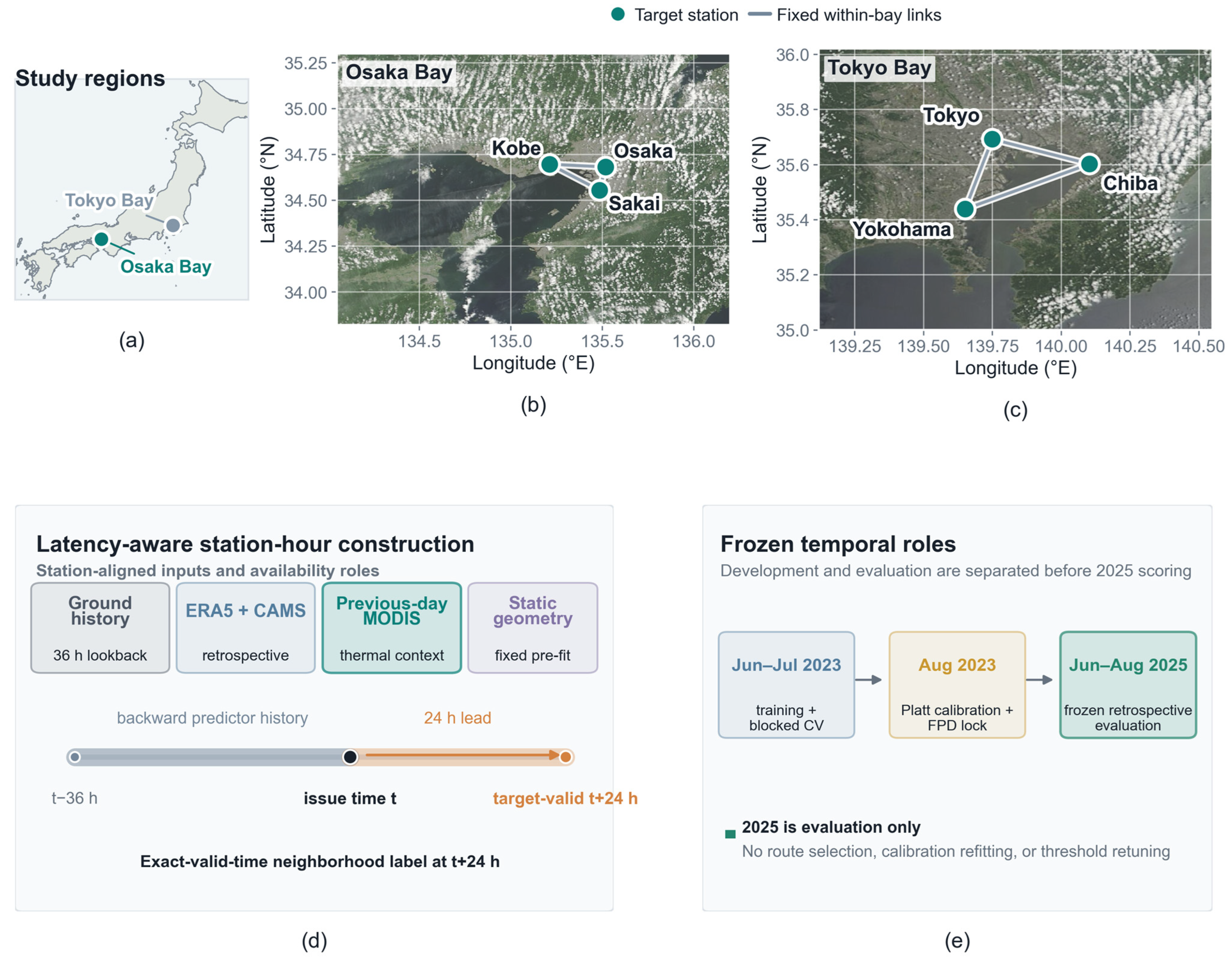
MODIS land-surface temperature (LST) is the primary satellite observation in the revised analysis. The main satellite route uses previous-day MODIS thermal context, separating satellite value from same-day availability assumptions. A dimension-matched timing experiment additionally compares same-day MODIS core18 and previous-day MODIS core18 routes using the same 18 MODIS variables. Sentinel-5P/TROPOMI products are retained for source-availability and coastal-coverage diagnostics but do not define the headline MODIS increment. All dynamic timestamps were converted to Japan Standard Time before assembling the station-hour table. The study uses products provided by Japan’s Ministry of the Environment and National Institute for Environmental Studies, the Copernicus Climate Data Store, ECMWF/Copernicus Atmosphere Data Store, NASA LAADS DAAC, and ESA/Copernicus Sentinel-5P services [11,12,13,14,15,16,17,18,19]. Source groups, native spatial and temporal support, station joins, quality-control rules, missing-state handling, and provider roles are summarized in Tables S1–S2. Figure 1 summarizes the coastal station networks, MODIS geographic context, and frozen temporal roles used throughout the analysis.

2.2. Compound-Warning Targets

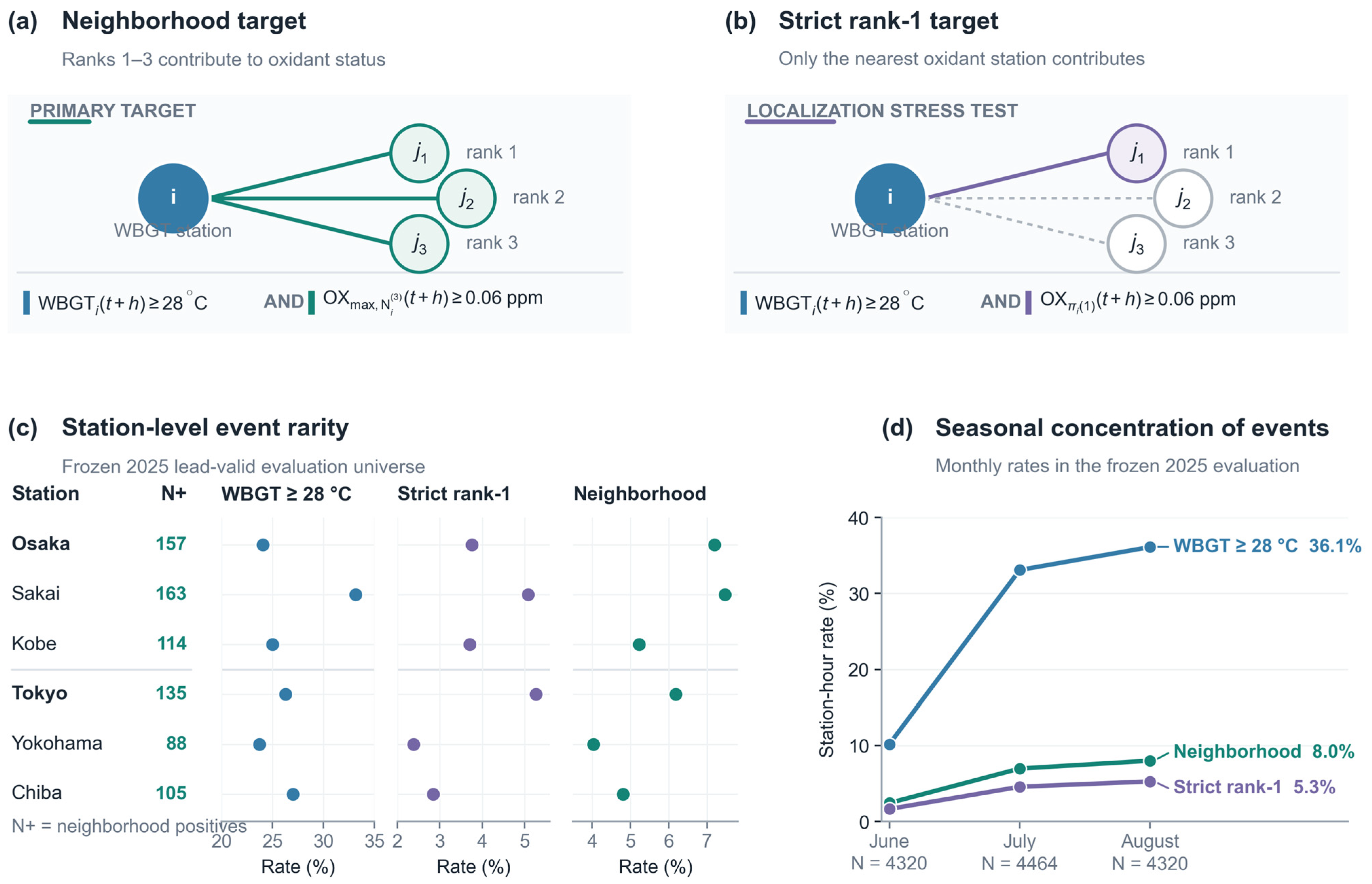
Let I denote the set of WBGT monitoring stations and J the set of photochemical-oxidant monitoring stations. For each WBGT station and hour, the humid-heat indicator equals one when WBGT is at least 28 °C. For each oxidant station and hour, the oxidant indicator equals one when the one-hour photochemical-oxidant concentration exceeds 0.06 ppm. Oxidant stations are ranked by geographic distance from each WBGT station, and the rank-K neighborhood contains its K nearest oxidant stations.
y i , t ( N , h ) = 1 { H i , t + h = 1 }   1 m a x j N i ( 3 ) O j , t + h = 1
Equation (1) defines the primary neighborhood target: humid heat is evaluated at the target WBGT station, while oxidant exceedance may occur at any of its three nearest oxidant stations. The strict nearest-station target is
y i , t ( S , h ) = 1 { H i , t + h = 1 }   1 { O π i ( 1 ) , t + h = 1 }
Both targets are exact-valid-time labels. A row issued at time t is positive only when the corresponding condition is observed at t + h, rather than at any time within a cumulative future window. The primary analysis focuses on the 24 h neighborhood target, which represents neighborhood-scale warning allocation. The strict rank-1 target is retained as a secondary localization stress test. Station neighborhoods are fixed before model fitting and are reported in the Supplementary Materials. Figure 2 illustrates the two target formulations and the station-level event distribution in the frozen 2025 evaluation universe.

2.3. Exact Temporal Protocol and Analytical Roles

The revised protocol separates model development, probability calibration, alert-threshold selection, and cross-year evaluation by issue time and target-valid time. A station-hour row belongs to a temporal role only when both timestamps remain inside the corresponding period. All 36 h input histories are backward-looking, and no feature at or after target-valid time is used as a predictor.
For the primary 24 h task, model fitting uses issue times from 1 June through 30 July 2023, whose target-valid times extend from 2 June through 31 July 2023. Hyperparameters and training duration are selected through blocked time-series validation within this training role. August 2023 is reserved for post-hoc calibration and false-alarm-budget threshold locking; it is not used for source-route, architecture, or graph-variant selection. The primary revised routes use all 4320 lead-valid calibration rows, including 99 positive rows (2.29% prevalence).
The retrospective cross-year evaluation uses issue times from 1 June through 30 August 2025, with target-valid times from 2 June through 31 August 2025. The full 24 h lead-valid universe contains 13,104 station-hour rows and 762 positive neighborhood-target rows. Model-specific paired contrasts are computed on identical row keys. All imputation, scaling, feature selection, class weighting, and source-specific preprocessing parameters are estimated within the 2023 training role; calibration parameters and alert thresholds are estimated from August 2023 predictions only. The 2025 period is a frozen retrospective cross-year evaluation rather than a model-selection source. The exact temporal roles and support sizes are summarized in Table 2.
Unless explicitly labeled as a forecast-consistent companion analysis, all headline results therefore represent a validation-locked hindcast benchmark.

2.4. Satellite Timing Routes and Matched Feature Bundles

The primary satellite estimand is the incremental warning value of previous-day MODIS thermal context beyond an otherwise identical non-satellite feature bundle. The non-satellite route contains recent ground history, ERA5 meteorology, CAMS composition, and static station geometry. The satellite route adds MODIS variables from the preceding local day while retaining the same rows, labels, model family, preprocessing protocol, calibration procedure, and false-alarm budgets. For metric M, the previous-day MODIS increment is
Δ M M O D I S = M ( G + E + C + D + M t 24 ) M ( G + E + C + D )
where G, E, C, D, and M denote ground/regime, ERA5, CAMS, static geometry, and MODIS feature groups, respectively. To separate timing from feature dimensionality, the same-day MODIS core18 and previous-day MODIS core18 routes contain the same 18 physical MODIS variables and differ only in temporal alignment. The matched timing effect is
Δ M t i m i n g = M ( G + E + C + D + M p r e v i o u s ( 18 ) ) M ( G + E + C + D + M c u r r e n t ( 18 ) )
The primary previous-day route retains valid-observation counts and MODIS quality variables. Rows without a valid previous-day observation remain in the model universe and are represented through training-fold median imputation and missingness indicators rather than being removed or replaced by future observations. This treatment prevents satellite availability from changing target support. The fitted imputation values and missingness encoding are applied unchanged to later roles. MODIS quality criteria, station aggregation, timing, and missing-state handling are summarized in Table S2. Table 3 defines the matched source routes used to estimate MODIS contribution.

2.5. Model Families and Matched Spatial Controls

XGBoost [20] is the primary estimator of satellite incremental value because it provides a strong nonlinear tabular baseline and supports exact source-bundle matching. Within each paired source contrast, the search space, temporal folds, and optimization budget were held fixed. The primary no-MODIS and previous-day MODIS routes each used 20 Optuna trials. The dimension-matched no-MODIS, same-day MODIS core18, and previous-day MODIS core18 routes each used an identical 80-trial protocol. For the dimension-matched timing contrast, the five highest-ranked candidates from each 80-trial blocked-CV study were combined using softmax weights derived from their training-only blocked-CV objective values. August 2023 was used only for post-hoc calibration and false-alarm-threshold locking, not for candidate selection or ensemble weighting. Final boosting rounds were determined from training-only blocked-CV performance. HGB, implemented with scikit-learn [21], is retained as a secondary boosted-tree reference. Analyses were implemented in Python 3.12.3 using NumPy 2.1.3, pandas 3.0.5, scikit-learn 1.9.0, XGBoost 3.4.0, Optuna 4.9.0, and PyTorch 2.5.1.
A 36 h Temporal FLOW model provides model-family confirmation. It applies a GRU encoder to station histories and produces horizon-specific warning probabilities. Its no-MODIS and previous-day MODIS routes share the same architecture, training schedule, and station-hour support, testing whether MODIS ranking value transfers from boosted trees to an explicitly temporal model. The model combines local, distance, and wind branches through a learned softmax router:
m i , t = α i , t l o c a l m i , t l o c a l + α i , t d i s t a n c e m i , t d i s t a n c e + α i , t w i n d m i , t w i n d , r α i , t r = 1
where the three non-negative routing weights sum to one. Router weights are retained for interpretation but are not used to select an operating point. Spatial structure is evaluated through four fixed-capacity controls: no graph, a static distance graph, a directional true-wind graph, and a joint distance–wind representation. These controls use identical source rows, base features, training budgets, and evaluation procedures. Spatial-shuffled, temporal-shuffled, reversed-wind, and edge-permuted controls are reported in the Supplementary Materials.
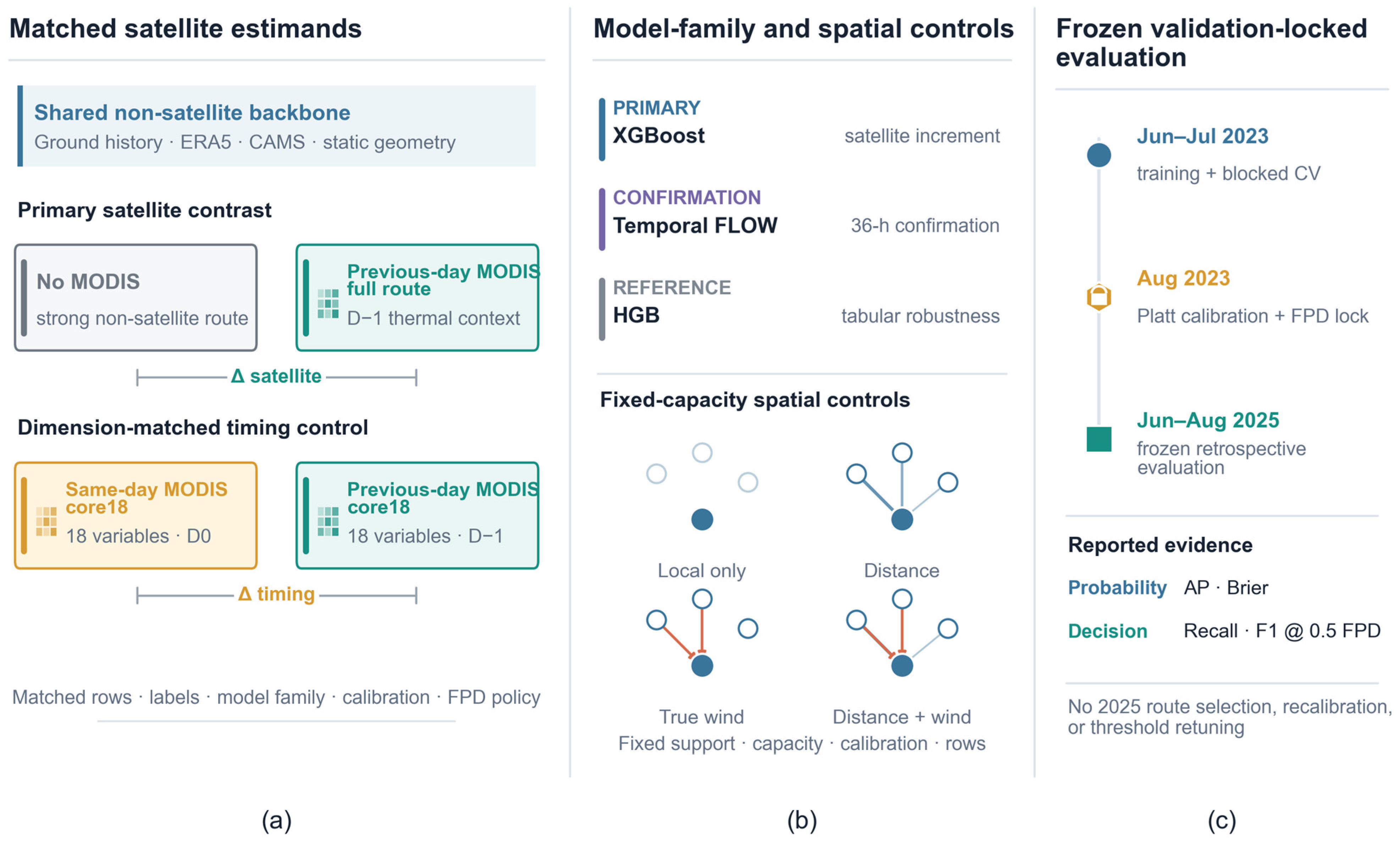
Simple warning references include current and lag-1 persistence, recent 24 h persistence, train-only station-hour climatology, and a WBGT-low-wind rule. They use the same temporal roles and validation-locked decision procedure as the learned models. Complete simple-baseline results under the revised temporal protocol are reported in Table S16. Source-route configurations, optimization details, frozen model-family results, graph controls, and simple-baseline results are reported in Tables S6–S8, S12, S13 and S16. Figure 3 summarizes the matched source routes, model-family and graph controls, and validation-locked evaluation design.

2.6. Training, Calibration, and Validation-Locked Alert Policies

All revised model fitting, hyperparameter selection, seed selection, ensemble weighting, calibration, and alert-threshold selection were conducted using the 2023 development and calibration roles only. The 2025 observations were used exclusively for the frozen retrospective evaluation of the finalized routes. Hyperparameters were selected through four expanding blocked time-series folds with forward temporal ordering and a 72 h embargo that separated model histories and future targets across adjacent folds. Matched source and graph comparisons used the same fold definitions and optimization budget. Preprocessing, imbalance parameters, early-stopping duration, and optimization settings were estimated from training-only folds. Final models were then refitted on the complete strict training role using frozen configurations. The Temporal FLOW confirmation used five prespecified final seeds and exponential moving-average weights.
Post-hoc probability calibration is fitted on August 2023 predictions only. Platt scaling is the primary calibration method [22]. For false-alarm budget b, the validation threshold is selected as
τ b = a r g m a x τ R e c a l l v a l ( τ ) s . t . F P D v a l ( τ ) b
where false alarms per station-day are defined as
F P D S ( τ ) = ( i , t ) S 1 { p ^ i , t ( h ) τ , y i , t ( h ) = 0 } N s t a t i o n d a y ( S )
The selected threshold is applied unchanged to the retrospective 2025 predictions. The primary decision operating point is 0.5 FPDs; 1.0 and 2.0 FPDs are secondary operating points. The 2025 rows are not used for test-time tie-breaking, threshold retuning, source-route selection, or calibration refitting.

2.7. Evaluation, Stratification, and Uncertainty

Probability quality is evaluated using Brier score [23] and average precision (AP) [24,25]. Decision performance is evaluated using precision, recall, and F1 after application of validation-locked FPD thresholds. Because event prevalence is low, accuracy and a default 0.5 probability cutoff are not used as primary evidence.
The primary uncertainty analysis uses paired Japan-local calendar-day bootstrap resampling with 10,000 replicates. Each sampled block retains all stations and hours from a selected calendar day, preserving shared coastal weather conditions across stations. Station-day, three-day moving-block, and seven-day moving-block intervals are reported as sensitivity analyses. The primary MODIS contrast, matched timing contrast, and primary graph contrasts are defined before evaluation; multiplicity within satellite and graph comparison families is controlled by the Holm procedure.
Prespecified satellite-value strata comprise all common rows, issue-time high- and lower-heat rows, rows with and without a valid previous-day MODIS observation, and the Osaka Bay and Tokyo Bay testbeds. These analyses estimate heterogeneity of the satellite increment; they do not select the headline model or alert threshold. Bay-specific performance and year-plus-bay transfer evaluate spatial domain shift across station geometry, event prevalence, satellite availability, and coastal thermal regimes without attributing the degradation to a single mechanism.

3. Results

3.1. Previous-Day MODIS Improves Validation-Locked Warning Decisions

The frozen 2025 cross-year evaluation contained 13,104 lead-valid station-hour rows, including 762 positive neighborhood-target rows. To isolate the decision value of satellite thermal observations, we compared two otherwise identical XGBoost routes: a strong non-satellite baseline containing ground history, ERA5 meteorology, CAMS composition, and static geometry, and a satellite route that additionally included previous-day MODIS thermal context.
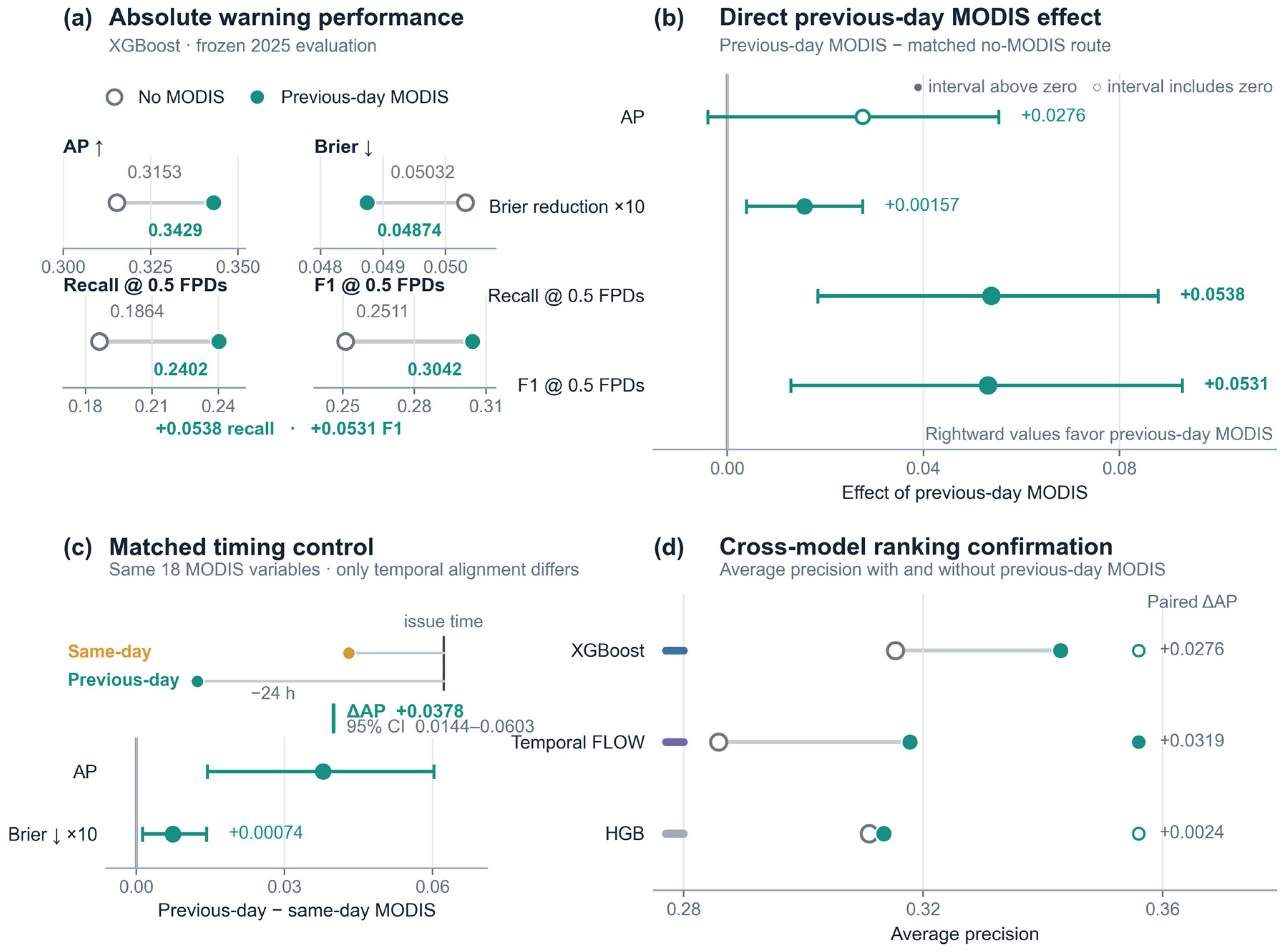
Table 4 reports absolute performance and paired differences. Holding the model family, non-satellite sources, temporal protocol, calibration route, and alert policy fixed, previous-day MODIS increased average precision (AP) from 0.3153 to 0.3429 and reduced the Brier score from 0.05032 to 0.04874. Under the prespecified budget of 0.5 FPDs, recall increased from 0.1864 to 0.2402 and F1 increased from 0.2511 to 0.3042. The improvement therefore spanned probability quality and validation-locked warning allocation: MODIS sharpened probabilistic discrimination, reduced squared probability error, and recovered more positive station-hours under the same validation-defined false-alarm constraint.
Paired Japan-local calendar-day resampling supported a Brier-score reduction of 0.00157 (95% CI: 0.00039–0.00276), a recall increase of 0.0538 (95% CI: 0.0184–0.0879), and an F1 increase of 0.0531 (95% CI: 0.0129–0.0928). All three effects remained supported after Holm adjustment within the prespecified primary satellite comparison family. The AP point estimate increased by 0.0276, with a wider calendar-day interval (95% CI: −0.0040–0.0554). The strongest all-row evidence thus appeared in the Brier score and low-FPD recovery, accompanied by a concordant positive shift in rare-event ranking.

3.2. A Dimension-Matched Timing Experiment Identifies the Previous-Day Advantage

The primary satellite route contains engineered MODIS summaries in addition to the non-satellite baseline. We therefore performed a dimension-matched timing experiment to determine whether the gain arose from temporal alignment rather than from a larger feature set. The same-day and previous-day routes used the same 18 MODIS variables, 80-trial search budget, blocked-CV-weighted top-5 ensemble procedure, and station-hour support; only the temporal alignment of the MODIS observations differed.
Under this matched design, previous-day MODIS increased AP from 0.3260 to 0.3638 and reduced the Brier score from 0.05141 to 0.05067 (Table 5). The paired AP increase was 0.0378 (95% CI: 0.0144–0.0603), and the Brier reduction was 0.000742 (95% CI: 0.000131–0.001422). Both effects remained positive when satellite feature dimension and model capacity were held fixed.
The matched experiment identifies source timing as a substantive component of the MODIS contribution. Previous-day LST provides a temporally stable surface thermal-memory signal, whereas same-day station-day joins can mix observations with different overpass and issue-time relationships. The advantage is therefore not explained by adding a larger satellite feature block; it reflects a more transferable temporal representation of the same remotely sensed thermal variables.

3.3. Temporal FLOW Reproduces the MODIS Ranking Gain

To test whether the MODIS effect depended on the boosted-tree estimator, we repeated the no-MODIS and previous-day MODIS comparison with a 36 h Temporal FLOW model using a gated recurrent unit encoder. The two FLOW routes shared the same temporal architecture, training schedule, graph-routing structure, and evaluation rows.
Previous-day MODIS increased Temporal FLOW AP from 0.2858 to 0.3178. The paired increase was 0.0319 (95% CI: 0.0019–0.0670), transferring the ranking benefit from XGBoost to an explicitly temporal neural model.
The thresholded operating metrics at 0.5 FPDs did not increase for the Temporal FLOW route, showing that conversion of improved ranking into low-budget alerts remained model-dependent. The cross-family result nevertheless confirms that previous-day MODIS sharpened rare-event ranking in both a boosted-tree model and a 36 h temporal encoder, while XGBoost realized the strongest low-budget allocation gains. Figure 4 summarizes the direct increment, timing control, and model-family confirmation; the HGB route is shown as a secondary boosted-tree reference.

3.4. Satellite Thermal Value Concentrates in High-Heat and Osaka Bay Conditions

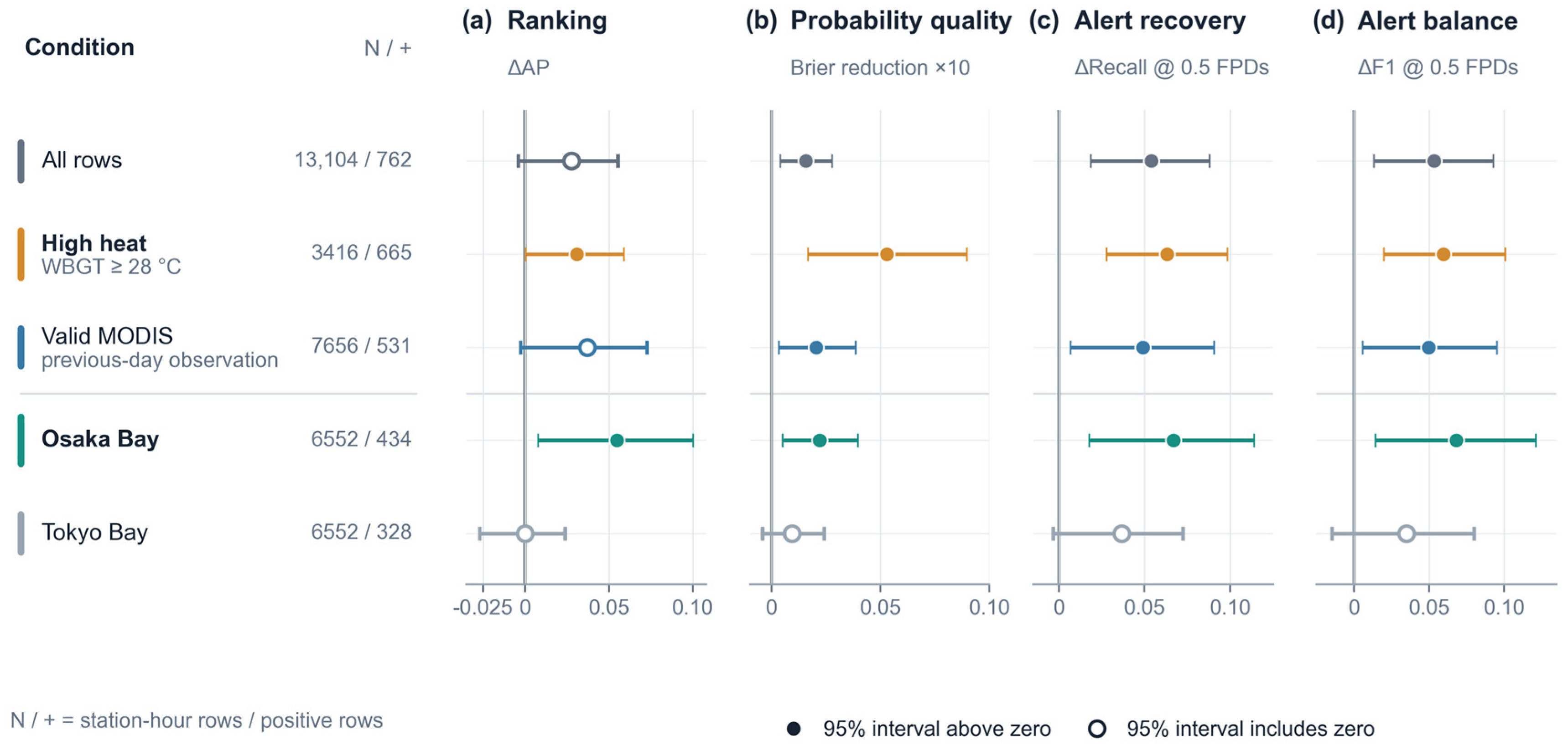
The previous-day MODIS increment was concentrated in prespecified environmental and geographic conditions. Its strongest effects appeared when the issue-time atmosphere was already thermally stressed. Among the 3416 station-hour rows with an issue-time WBGT ≥ 28 °C, including 665 future positive rows, previous-day MODIS increased AP by 0.0310 (95% CI: 0.00035–0.05890), reduced the Brier score by 0.00528 (95% CI: 0.00166–0.00896), and increased recall and F1 at 0.5 FPDs by 0.0632 (95% CI: 0.0276–0.0983) and 0.0595 (95% CI: 0.0197–0.1006), respectively. The satellite contribution was therefore largest in the high-heat regime, which contained 665 of the 762 compound-warning positives in the common-row evaluation universe.
The source-availability analysis produced a consistent pattern. Among the 7656 rows with a valid previous-day MODIS observation, including 531 positive rows, the Brier-score reduction was 0.00205 (95% CI: 0.00032–0.00385), while recall and F1 increased by 0.0490 (95% CI: 0.0065–0.0904) and 0.0497 (95% CI: 0.0055–0.0950). AP increased by 0.0371, with a wider interval (95% CI: −0.0027–0.0726). Thus, when a previous-day thermal observation was available, the clearest gains appeared in probability quality and low-budget event recovery, accompanied by a positive ranking shift.
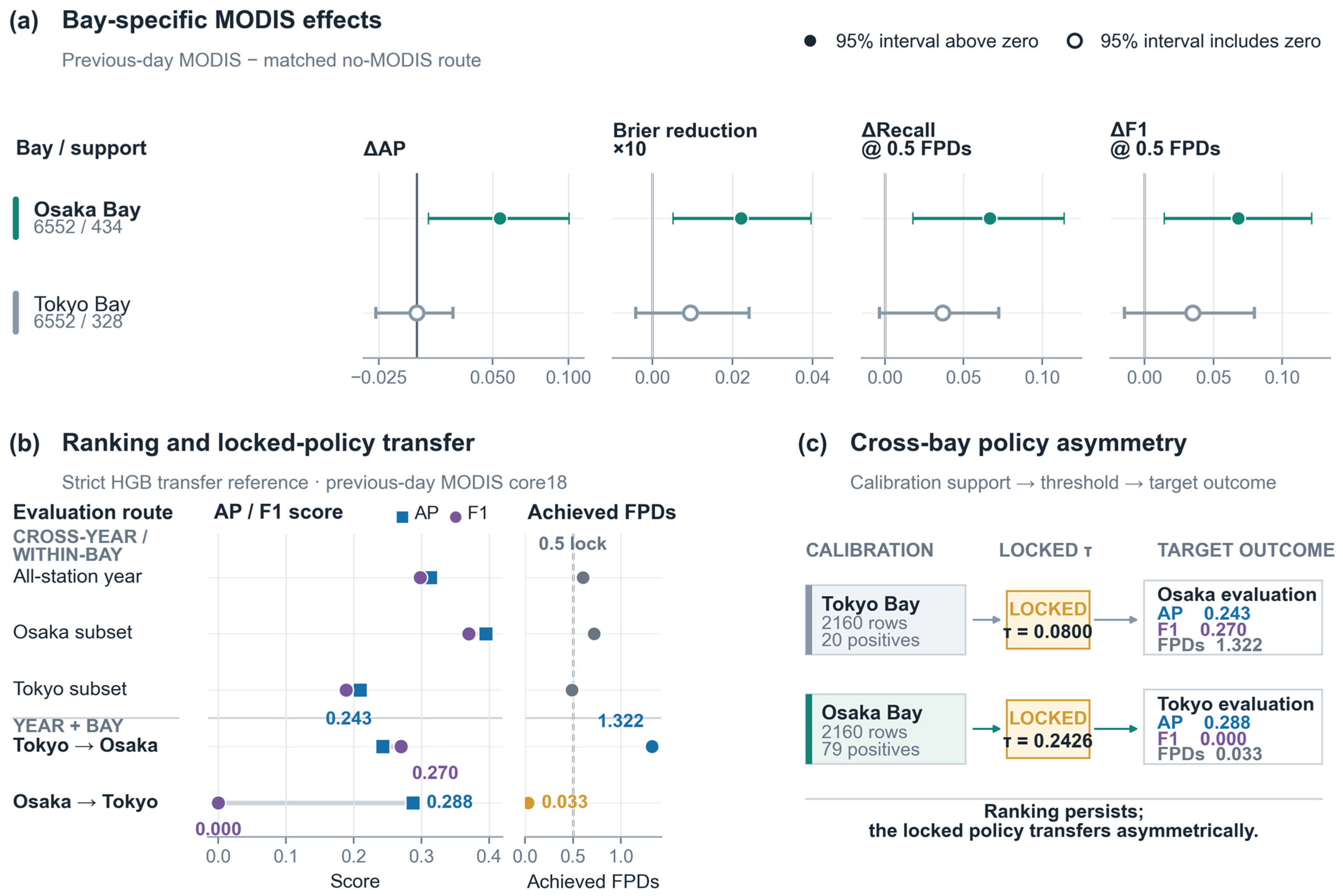
The satellite increment was also geographically structured (Table 6 and Figure 5). In Osaka Bay, previous-day MODIS increased AP by 0.0548 (95% CI: 0.0077–0.1002), reduced the Brier score by 0.00221 (95% CI: 0.00051–0.00396), and increased recall and F1 at 0.5 FPDs by 0.0668 (95% CI: 0.0175–0.1140) and 0.0680 (95% CI: 0.0140–0.1212), respectively. The corresponding ranking increment in Tokyo Bay was close to zero, although the decision-metric point estimates remained positive. The strongest MODIS increments were therefore localized to high-heat station-hours and the Osaka Bay testbed, revealing a structured rather than uniform satellite contribution.

3.5. Distance-Based Coastal Context Provides the Most Stable Spatial Gain

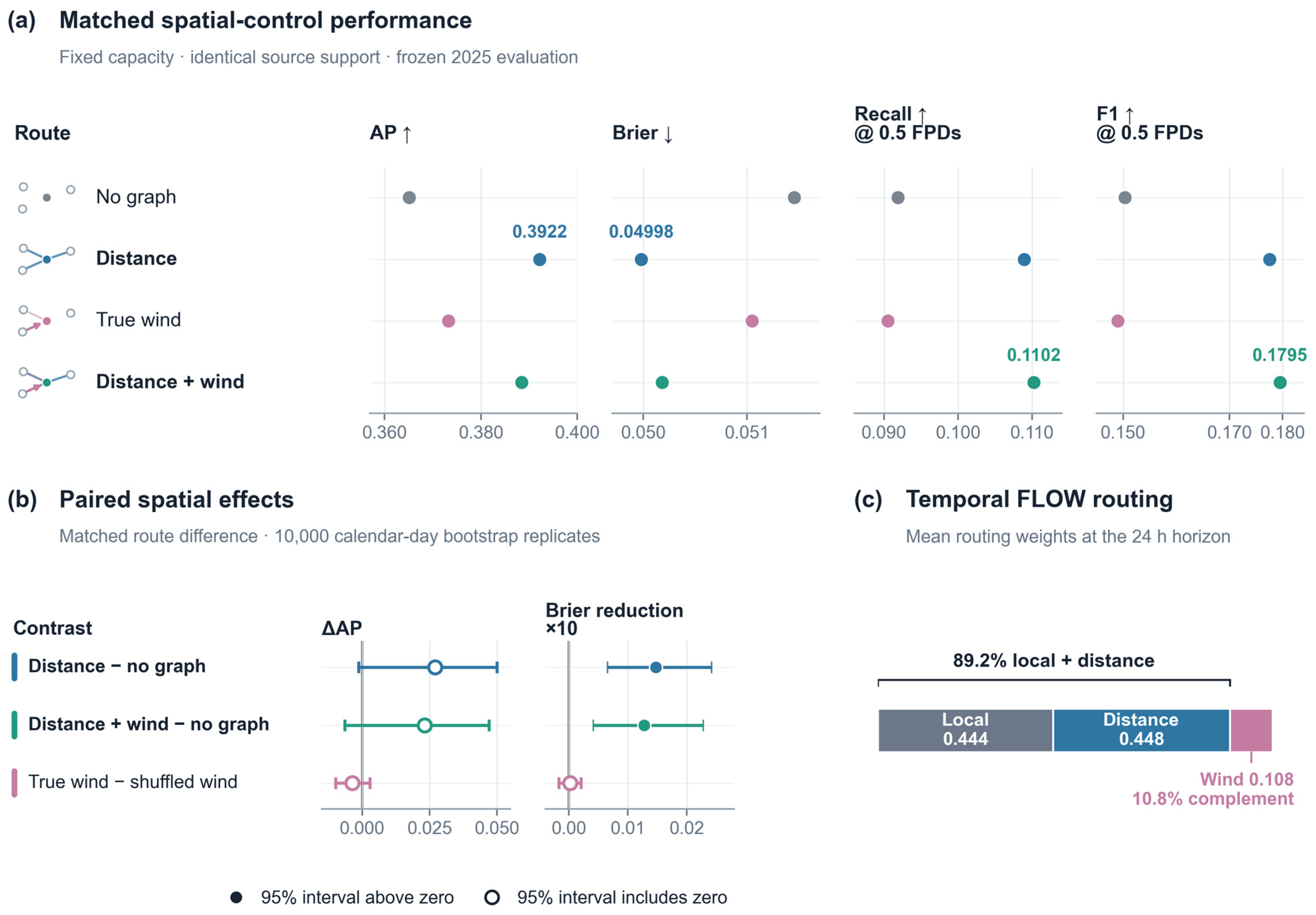
Fixed-capacity graph controls separated the contribution of stable coastal geometry from directional wind alignment (Table 7 and Figure 6). Without graph-derived spatial context, XGBoost achieved an AP of 0.3652 and a Brier score of 0.05145. Adding a static distance graph increased AP to 0.3922 and reduced the Brier score to 0.04998. The paired Brier reduction relative to the no-graph route was 0.00147 (95% CI: 0.00065–0.00241), and this probability-quality improvement remained supported after Holm adjustment within the graph comparison family.
The joint distance–wind representation achieved the highest low-budget decision point estimates, with recall/F1 of 0.1102/0.1795 compared with 0.0919/0.1504 for the no-graph route. Its Brier score decreased to 0.05018, corresponding to a paired reduction of 0.00127 (95% CI: 0.00041–0.00228). The distance-only and joint routes therefore provided consistent evidence that spatial neighborhood information improves 24 h probability quality, while the joint representation retained the highest low-budget recall and F1.
Directional wind alignment did not provide a standalone 24 h advantage over the spatially shuffled wind control. The true-wind route changed AP by −0.0037 relative to the shuffled-wind route (95% CI: −0.0099–0.0028), and its thresholded recall and F1 point estimates were lower. The matched controls therefore identify stable station proximity, rather than directional wind alignment alone, as the principal spatial contributor at the 24 h horizon.
The Temporal FLOW router produced the same structural interpretation. In the previous-day MODIS route, the mean routing weights were 0.444 for local context, 0.448 for distance-based context, and 0.108 for the wind branch. The learned model therefore allocated 89.2% of its average routing mass to local and distance information and used wind alignment as a lower-weight complement. Together, the matched controls and learned routing weights support a horizon-specific spatial design in which coastal proximity provides the stable backbone and wind information supplies selective contextual refinement.

3.6. Bay-Specific Heterogeneity Produces an Asymmetric Transfer Bottleneck

The bay-specific MODIS analysis revealed a pronounced geographic asymmetry. Osaka Bay contained 434 positive rows among 6552 station-hour rows (prevalence, 6.62%), whereas Tokyo Bay contained 328 positives among the same number of rows (prevalence, 5.01%). Previous-day MODIS produced a supported AP increase of 0.0548 in Osaka Bay but an essentially unchanged AP in Tokyo Bay. The Brier, recall, and F1 increments were likewise larger and more stable in Osaka Bay.
This heterogeneity was examined with HGB previous-day MODIS core18 transfer tests under the same strict temporal roles as the primary analysis. Under all-station 2023-to-2025 transfer, 24 h neighborhood F1 was 0.2980. When the same model and locked threshold were evaluated by bay, Osaka Bay retained an F1 of 0.3700, whereas Tokyo Bay achieved 0.1886. Simultaneous year-plus-bay transfer remained strongly asymmetric: training and calibrating on Tokyo Bay before testing on Osaka Bay produced an F1 of 0.2699, while the reverse Osaka-to-Tokyo route produced an F1 of 0.0000.
The strict transfer protocol used 8430 all-station fitting rows, 4320 all-station calibration rows, and 13,104 frozen test rows. Cross-bay routes used 4215 fitting rows and 2160 calibration rows from the source bay and 6552 test rows from the target bay. Bay-specific positive counts remained 434 in Osaka Bay and 328 in Tokyo Bay. The two source-bay calibration sets also differed in event support: the Tokyo Bay calibration period contained 20 positive rows, whereas the Osaka Bay calibration period contained 79. This asymmetry contributed to markedly different locked thresholds and helps explain why ranking information persisted under Osaka-to-Tokyo transfer even when the transferred alert policy issued almost no positive decisions.
The Osaka-to-Tokyo transfer collapse did not correspond to a complete loss of ranking information. Its AP remained 0.2876 even when the thresholded F1 fell to 0.0000; the reverse Tokyo-to-Osaka route achieved AP/F1 of 0.2428/0.2699. This divergence suggests that at least part of the cross-bay bottleneck arises from transferring a fixed score scale and alert threshold across different bay-specific event prevalences and predictor distributions, rather than from the disappearance of all discriminative signal.
The results therefore identify two connected forms of spatial heterogeneity. First, previous-day MODIS contributes more strongly in Osaka Bay than in Tokyo Bay. Second, a validation-locked alert policy does not automatically transfer between the two bay systems even when useful ranking information remains. Cross-bay degradation is therefore expressed at both the representation and decision-policy layers (Figure 7).

4. Discussion

4.1. Remote-Sensing Value at the Warning-Decision Layer

The central result of this study is that remotely sensed thermal information can change a warning decision even after recent ground observations, meteorological reanalysis, and atmospheric-composition context have already been supplied to a strong nonlinear model. This distinction is important because the inclusion of a satellite product in a multimodal feature stack does not, by itself, establish remote-sensing value. Satellite value is demonstrated when an otherwise matched warning route improves after the satellite observation is added.
The previous-day MODIS comparison provides that direct evidence. Relative to the ground–ERA5–CAMS route, MODIS improved probability quality and recovered more positive station-hours under the validation-locked low-false-alarm policy. The dimension-matched core18 experiment strengthens this interpretation: previous-day MODIS outperformed the same-day version of the same 18 physical variables, so the ranking improvement cannot be attributed to a larger satellite feature space or a more flexible model. The result identifies temporal placement of the satellite observation as part of its predictive value.
This finding extends the role of remote sensing beyond concentration reconstruction. Satellite-enhanced air-quality studies commonly evaluate whether Earth-observation variables reduce concentration-estimation error [3,4,5,6,7,8]. The present results address a different question: whether the satellite observation changes the ordering and allocation of future compound-warning risk under a policy whose false-alarm tolerance is fixed before evaluation. Improvements in Brier score, recall, and F1 show that the MODIS contribution is visible not only in threshold-free ranking, but also in the probability and decision layers that govern warning use.
The use of a strong non-satellite baseline is essential to this conclusion. ERA5 contains variables closely related to humid heat, radiation, atmospheric mixing, stagnation, and transport, while CAMS provides broad composition context. MODIS therefore does not replace meteorological information. It contributes a distinct surface thermal state that remains informative after atmospheric predictors have been accounted for. The relevant scientific claim is consequently not that satellite observations dominate meteorology, but that latency-aware thermal remote sensing adds measurable decision information beyond recent ground, meteorological, composition, and geometric context.

4.2. Previous-Day MODIS as Surface Thermal Memory

The superiority of the previous-day route over the same-day matched route suggests that the most transferable MODIS signal is not an instantaneous substitute for issue-time air temperature. Instead, MODIS LST appears to provide surface thermal-memory information that complements the hourly atmospheric state.
Land-surface temperature integrates processes that are only partially represented by near-surface meteorological variables, including heat storage in built materials, surface moisture availability, vegetation and impervious-surface contrasts, and the release of accumulated heat over the subsequent diurnal cycle. A previous-day observation can therefore summarize the thermal state from which the next day’s humid-heat and photochemical environment develops in the coupled setting documented by compound heat–ozone studies [1,2]. This interpretation is consistent with the dimension-matched AP and Brier improvements, although the present analysis identifies predictive information rather than an isolated surface-energy mechanism.
The environmental stratification provides additional support for this interpretation. The largest MODIS increments occurred when issue-time WBGT was already at or above 28 °C. Under these conditions, atmospheric heat stress was established, and remotely sensed surface temperature supplied information about the persistence and spatial intensity of the underlying thermal environment. The substantially larger Brier-score reduction in the high-heat subset indicates that MODIS contributes most when the warning problem is already close to the compound-event regime, rather than acting as a uniform correction across all station-hours.
The timing result also clarifies why the same-day route is not necessarily the most informative option for warning. A station-day same-day join can combine issue times that occur before and after the relevant satellite overpass and can therefore represent different availability states within the same calendar day. When available, previous-day MODIS defines a consistently ordered pre-issue thermal observation and avoids mixing issue times that occur before and after the same-day overpass. Its advantage is therefore both statistical and timing-aware: it supplies a temporally stable signal while removing same-day overpass-order ambiguity.
The ranking improvement reproduced by the 36 h Temporal FLOW model further indicates that the effect is not specific to boosted trees. XGBoost converted the MODIS signal most effectively into low-FPD warning gains, whereas Temporal FLOW reproduced the AP improvement. This pattern shows that the satellite ranking signal transfers across model families, while its conversion into a particular alert policy depends on the model’s score distribution and calibration. More broadly, satellite contribution should be evaluated separately at the ranking, probability, and thresholded-decision layers rather than summarized by one aggregate performance measure.

4.3. Spatial Context, Bay Heterogeneity, and Policy Transfer

The matched graph controls revise the interpretation of spatial context in coastal compound warning. At the 24 h horizon, the most stable improvement came from static distance-based structure rather than from directional wind alignment alone. Distance encodes persistent properties of the monitoring network and coastal environment: neighborhood proximity, shared urban background, regional-scale heat exposure, and spatially coherent oxidant regimes. These properties remain relevant over a daily forecast horizon even when the instantaneous wind direction changes.
The Temporal FLOW router reached the same conclusion through learned allocation. Local and distance branches received 44.4% and 44.8% of the average routing mass, respectively, while the wind branch received 10.8%. The model did not discard wind information; it used it selectively as a complementary source of context. This supports a horizon-adaptive interpretation of spatial modeling. Directional transport may become more informative at shorter horizons, which remains a useful direction for lead-specific graph evaluation; at 24 h, warning benefits more consistently from stable local and proximity-based structure.
This result also explains why a physically plausible wind graph need not outperform distance-based or shuffled controls at the 24 h horizon [9,10]. Issue-time wind is one realization within a daily evolution of sea-breeze reversal, synoptic forcing, boundary-layer development, and changing photochemistry. A single directional relation is therefore a partial description of the 24 h source–receptor process. The stronger result is not that wind is irrelevant, but that it should enter as one routed component within a broader spatial representation rather than being imposed as the sole organizing graph.
Bay-specific MODIS effects reveal a second form of spatial structure. The satellite increment was concentrated in Osaka Bay and was much smaller in Tokyo Bay. This difference is consistent with variation in urban surface composition, coastline orientation, monitoring geometry, event prevalence, satellite sampling conditions, and local meteorological regimes. The current results do not isolate one factor, but they show that satellite contribution is geographically conditional and cannot be assumed to transfer unchanged between coastal systems.
The transfer results further distinguish representation transfer from policy transfer. In the most difficult Osaka-to-Tokyo route, AP remained materially above an uninformative ranking even though F1 under the transferred threshold approached zero. Useful ordering information therefore persisted, but the score scale and locked alert threshold did not transfer with equal success. This divergence indicates that cross-bay deployment requires both transferable representations and locally aligned decision policies.
Three improvements follow directly from this finding. First, coastal geometry can be normalized using bay-relative coordinates, coastline orientation, station density, and distance-to-coast descriptors. Second, multi-bay training can encourage representations that retain common thermal and meteorological structure without encoding one station layout too strongly. Third, a target bay should provide a limited calibration period for probability and threshold adaptation, even when the forecasting representation is transferred without retraining. These steps address the distinct representation and policy components of the observed transfer bottleneck.

4.4. Study Scope and Operational Pathway

The present study establishes a retrospective, validation-locked benchmark for quantifying the decision value of satellite thermal observations. Its strongest evidence concerns the 24 h neighborhood target, previous-day MODIS, and six stations across two Japanese coastal bays. These design choices provide controlled source and timing comparisons, while additional years, coastal regions, and monitoring configurations are needed to establish broader geographic and climatic generality.
The benchmark uses retrospective ERA5 and CAMS context. A fully forecast-consistent companion route should replace these fields with forecasts initialized before issue time, retain previous-day or overpass-gated satellite inputs, and recalibrate probability and FPD thresholds under the same source-availability policy. The previous-day route removes same-day overpass ambiguity because the underlying observation precedes the warning issue time. Operational use would still require verification that the corresponding product is released and quality-controlled before each issue time.
The current evidence is also specific to the MODIS thermal context. Sentinel-5P/TROPOMI remains valuable for composition and coastal-coverage diagnostics, but a primary TROPOMI warning contribution would require source-matched experiments with stable QA-valid coverage and explicit overpass-age control. Keeping these questions separate preserves a clear distinction between demonstrated thermal value and prospective composition value.
Probability estimates in the present benchmark are most appropriately used for ranking and validation-locked alert allocation. Multi-season calibration, prospective replay, and operator-defined cost functions are the next steps toward absolute-risk communication. A practical deployment pathway would therefore proceed through a shadow-mode system: forecast-consistent inputs generate station-hour risk rankings, source-availability flags identify the evidence supporting each score, and human operators review alerts under a predefined burden budget before public warning use.
The broader contribution is a remote-sensing evaluation principle. Satellite observations should not be credited because they are present in a multimodal model; they should be credited when a temporally valid observation improves a matched decision route. By combining direct source contrasts, matched timing, validation-locked policies, and dependence-aware uncertainty, the present framework provides a reproducible way to measure that contribution.

5. Conclusions

This study evaluated whether a temporally available satellite thermal observation changes a coastal compound-warning decision after strong ground, meteorological, and atmospheric-composition predictors have already been provided. Through CoAST-EWS Japan, the analysis connected remotely sensed surface thermal context to lead-specific warning probabilities and validation-locked false-alarm policies across six stations in Osaka Bay and Tokyo Bay.
Previous-day MODIS produced a clear decision-layer increment beyond the ground–ERA5–CAMS baseline. It reduced the Brier score and increased recall and F1 under the budget of 0.5 FPDs, while also producing a positive AP shift. The dimension-matched timing experiment provided the strongest identification: using the same 18 MODIS variables, previous-day context increased AP over the same-day route by 0.0378, with a 95% calendar-day interval of 0.0144–0.0603. The MODIS ranking increment was also reproduced by a 36 h Temporal FLOW model, showing that the thermal signal was not specific to the boosted-tree estimator.
The satellite contribution was environmentally and geographically structured. Its largest gains occurred during high-heat issue times and in Osaka Bay, supporting an interpretation of MODIS LST as surface thermal-memory context rather than as a uniform replacement for atmospheric predictors. Matched spatial controls further showed that distance-based coastal structure supplied the most stable 24 h graph-related probability improvement. The learned router retained wind-aligned information as a low-weight complement, but did not use it as the sole organizing principle for daily-horizon spatial dependence.
The broader contribution is a decision-oriented remote-sensing evaluation framework. Satellite observations should be credited when a temporally valid source improves an otherwise matched warning route, not simply because it is included in a multimodal model. Extending this framework to forecast-consistent meteorology, additional coastal regions, multi-season calibration, and stricter station-level localization will establish how the demonstrated MODIS thermal value transfers from retrospective validation to prospective warning use.

Supplementary Materials

The following supporting information can be downloaded at: https://www.mdpi.com/article/10.3390/rs18172874/s1.

Author Contributions

Conceptualization, J.T. and R.S.; methodology, J.T.; software, J.T.; validation, J.T.; formal analysis, J.T.; investigation, J.T.; resources, R.S.; data curation, J.T.; writing—original draft preparation, J.T.; writing—review and editing, J.T. and R.S.; visualization, J.T.; supervision, R.S.; project administration, R.S. All authors have read and agreed to the published version of the manuscript.

Funding

This research received no external funding.

Data Availability Statement

The original contributions presented in the study are included in the article and Supplementary Materials; further inquiries can be directed to the corresponding author.

Acknowledgments

The authors acknowledge the Ministry of the Environment, Japan, and the National Institute for Environmental Studies for ground WBGT and photochemical-oxidant data; the European Centre for Medium-Range Weather Forecasts and the Copernicus Climate Change Service for ERA5; the Copernicus Atmosphere Monitoring Service for atmospheric-composition data; NASA LAADS DAAC for MODIS products; and the European Space Agency and the Copernicus Programme for Sentinel-5P/TROPOMI products. We acknowledge the use of imagery provided by services from NASA’s Global Imagery Browse Services (GIBS), part of NASA’s Earth Observing System Data and Information System (EOSDIS).

Conflicts of Interest

The authors declare no conflicts of interest.

Abbreviations

The following abbreviations are used in this manuscript:
AbbreviationDefinition
APAverage Precision
CAMSCopernicus Atmosphere Monitoring Service
ERA5ECMWF Reanalysis v5
FPDsFalse Alarms Per Station-Day
HGBHistogram Gradient Boosting
LSTLand-Surface Temperature
MODISModerate Resolution Imaging Spectroradiometer
OXPhotochemical Oxidants
TROPOMITropospheric Monitoring Instrument
WBGTWet-Bulb Globe Temperature
XGBoostExtreme Gradient Boosting

References

  1. Zhou, X.; Li, M.; Huang, X.; Liu, T.; Zhang, H.; Qi, X.; Wang, Z.; Qin, Y.; Geng, G.; Wang, J.; et al. Urban Meteorology–Chemistry Coupling in Compound Heat–Ozone Extremes. Nat. Cities 2025, 2, 847–856. [Google Scholar] [CrossRef] [Scilit]
  2. Schnell, J.L.; Prather, M.J. Co-Occurrence of Extremes in Surface Ozone, Particulate Matter, and Temperature over Eastern North America. Proc. Natl. Acad. Sci. USA 2017, 114, 2854–2859. [Google Scholar] [CrossRef] [Scilit]
  3. Wang, W.; Liu, X.; Bi, J.; Liu, Y. A Machine Learning Model to Estimate Ground-Level Ozone Concentrations in California Using TROPOMI Data and High-Resolution Meteorology. Environ. Int. 2022, 158, 106917. [Google Scholar] [CrossRef] [Scilit]
  4. Song, G.; Li, S.; Xing, J.; Yang, J.; Dong, L.; Lin, H.; Teng, M.; Hu, S.; Qin, Y.; Zeng, X. Surface UV-Assisted Retrieval of Spatially Continuous Surface Ozone with High Spatial Transferability. Remote Sens. Environ. 2022, 274, 112996. [Google Scholar] [CrossRef] [Scilit]
  5. Li, T.; Yang, Q.; Wang, Y.; Wu, J. Joint Estimation of PM2.5 and O3 over China Using a Knowledge-Informed Neural Network. Geosci. Front. 2023, 14, 101499. [Google Scholar] [CrossRef] [Scilit]
  6. Zhou, X.; Liang, X.; Zhu, Q.; Gu, J.; Guan, Q. A Multiscale Spatial-Temporal-Variable Feature Fusion Network for Predicting Multiple Air Pollutants. Environ. Int. 2025, 205, 109864. [Google Scholar] [CrossRef] [Scilit]
  7. Mamic, L.; Pirotti, F. Harnessing Open Remote Sensing Data and Machine Learning for Daily Ground-Level Ozone Prediction Models: Spatio-Temporal Insights in the Continental Biogeographical Region. Atmos. Pollut. Res. 2025, 16, 102514. [Google Scholar] [CrossRef] [Scilit]
  8. Ding, Y.; Li, S.; Xing, J.; Li, X.; Ma, X.; Song, G.; Teng, M.; Yang, J.; Dong, J.; Meng, S. Retrieving Hourly Seamless PM2.5 Concentration Across China with Physically Informed Spatiotemporal Connection. Remote Sens. Environ. 2024, 301, 113901. [Google Scholar] [CrossRef] [Scilit]
  9. Wu, W.; Mo, X.; Li, H. A Novel Wind-Aware Dynamic Graph Neural Network for Urban Ground-Level Ozone Concentration Prediction. ISPRS Int. J. Geo-Inf. 2026, 15, 101. [Google Scholar] [CrossRef] [Scilit]
  10. Wang, Y.; Cheng, K.; Tian, S.; Xu, S.; Zhang, P. SSL-MSGA-CTFormer: A Neighborhood-Based Spatiotemporal Air Quality Inference Model Integrating Dynamic Multi-Scale Graph Attention and Self-Supervised Learning. J. Clean. Prod. 2026, 554, 148064. [Google Scholar] [CrossRef] [Scilit]
  11. Hersbach, H.; Bell, B.; Berrisford, P.; Hirahara, S.; Horanyi, A.; Munoz-Sabater, J.; Nicolas, J.; Peubey, C.; Radu, R.; Schepers, D.; et al. The ERA5 Global Reanalysis. Q. J. R. Meteorol. Soc. 2020, 146, 1999–2049. [Google Scholar] [CrossRef] [Scilit]
  12. Copernicus Climate Data Store. ERA5 Hourly Data on Single Levels from 1940 to Present. 2026. Available online: https://cds.climate.copernicus.eu/datasets/reanalysis-era5-single-levels (accessed on 26 May 2026).
  13. NASA LAADS DAAC. MOD11A1: MODIS/Terra Land Surface Temperature/Emissivity Daily L3 Global 1km SIN Grid. 2026. Available online: https://ladsweb.modaps.eosdis.nasa.gov/missions-and-measurements/products/MOD11A1/ (accessed on 26 May 2026).
  14. ECMWF. CAMS Global Atmospheric Composition Forecasts. 2026. Available online: https://www.ecmwf.int/en/forecasts/dataset/cams-global-atmospheric-composition-forecasts (accessed on 26 May 2026).
  15. Copernicus Atmosphere Data Store. CAMS Global Atmospheric Composition Forecasts. 2026. Available online: https://ads.atmosphere.copernicus.eu/datasets/cams-global-atmospheric-composition-forecasts (accessed on 26 May 2026).
  16. Veefkind, J.P.; Aben, I.; McMullan, K.; Foerster, H.; de Vries, J.; Otter, G.; Claas, J.; Eskes, H.J.; de Haan, J.F.; Kleipool, Q.; et al. TROPOMI on the ESA Sentinel-5 Precursor: A GMES Mission for Global Observations of the Atmospheric Composition for Climate, Air Quality and Ozone Layer Applications. Remote Sens. Environ. 2012, 120, 70–83. [Google Scholar] [CrossRef] [Scilit]
  17. European Space Agency Sentinel-5P. Data Products. 2026. Available online: https://www.esa.int/Applications/Observing_the_Earth/Copernicus/Sentinel-5P/Data_products (accessed on 26 May 2026).
  18. Ministry of the Environment, Government of Japan. Heat Illness Prevention Information: About WBGT. 2026. Available online: https://www.wbgt.env.go.jp/en/sp/wbgt.php (accessed on 26 May 2026).
  19. Ministry of the Environment, Government of Japan. Environmental Quality Standards in Japan: Air Quality. 2026. Available online: https://www.env.go.jp/en/air/aq/aq.html (accessed on 26 May 2026).
  20. Chen, T.; Guestrin, C. XGBoost: A Scalable Tree Boosting System. In Proceedings of the 22nd ACM SIGKDD International Conference on Knowledge Discovery and Data Mining, San Francisco, CA, USA, 13–17 August 2016; pp. 785–794. [Google Scholar]
  21. Pedregosa, F.; Varoquaux, G.; Gramfort, A.; Michel, V.; Thirion, B.; Grisel, O.; Blondel, M.; Prettenhofer, P.; Weiss, R.; Dubourg, V.; et al. Scikit-Learn: Machine Learning in Python. J. Mach. Learn. Res. 2011, 12, 2825–2830. [Google Scholar]
  22. Guo, C.; Pleiss, G.; Sun, Y.; Weinberger, K.Q. On Calibration of Modern Neural Networks. In Proceedings of the 34th International Conference on Machine Learning, Sydney, Australia, 6–11 August 2017; Volume 70, pp. 1321–1330. [Google Scholar]
  23. Brier, G.W. Verification of Forecasts Expressed in Terms of Probability. Mon. Weather Rev. 1950, 78, 1–3. [Google Scholar] [CrossRef] [Scilit]
  24. Davis, J.; Goadrich, M. The Relationship Between Precision-Recall and ROC Curves. In Proceedings of the 23rd International Conference on Machine Learning, Pittsburgh, PA, USA, 25–29 June 2006; pp. 233–240. [Google Scholar]
  25. Saito, T.; Rehmsmeier, M. The Precision-Recall Plot Is More Informative Than the ROC Plot When Evaluating Binary Classifiers on Imbalanced Datasets. PLoS ONE 2015, 10, e0118432. [Google Scholar] [CrossRef] [Scilit] [PubMed]
Figure 1. Spatial context and latency-aware analytical design of CoAST-EWS Japan. (a) National locator of the Osaka Bay and Tokyo Bay study regions. (b) Osaka Bay station network comprising Kobe, Osaka, and Sakai, with fixed within-bay links over Earth-observation geographic context. (c) Tokyo Bay station network comprising Tokyo, Yokohama, and Chiba, with the same fixed-link representation. (d) Construction of station-hour samples from a 36 h ground-observation history, retrospective ERA5/CAMS context, previous-day MODIS thermal context, and fixed geometry; the neighborhood label is evaluated at the exact target-valid time, t + 24 h. (e) Frozen temporal roles: June–July 2023 for training and blocked cross-validation, August 2023 for Platt calibration and false-alarm-budget locking, and June–August 2025 for frozen retrospective evaluation. Backgrounds in (b,c) are NASA EOSDIS GIBS Terra/MODIS corrected-reflectance true-color daily composites for 21 July 2025; they provide geographic context only and do not supply quantitative values.
Remotesensing 18 02874 g001
Figure 2. Compound-warning target definitions and event rarity in the frozen 2025 lead-valid evaluation universe. (a) Primary rank-1-to-rank-3 neighborhood target, in which humid-heat exceedance at station i is combined with oxidant exceedance at any of its three fixed nearest oxidant stations. (b) Strict rank-1 localization stress test, in which oxidant exceedance is required at the nearest station only. Colored solid links denote oxidant stations included in each target; gray dashed links are excluded. (c) Station-specific humid-heat, strict rank-1, and neighborhood event rates, with neighborhood positive counts. (d) Monthly station-hour rates from June to August 2025. Rates in panels (c,d) are calculated from the same canonical lead-valid evaluation support used in the corresponding target audit.
Remotesensing 18 02874 g002
Figure 3. Matched satellite estimands, model-family and spatial controls, and frozen validation-locked evaluation. (a) The primary source contrast compares the no-MODIS route with the previous-day MODIS full route, whereas a separate dimension-matched core18 comparison isolates same-day versus previous-day timing using the same 18 MODIS variables. (b) XGBoost estimates the primary satellite increment, Temporal FLOW provides a 36 h model-family confirmation, HGB serves as a secondary tabular reference, and fixed-capacity spatial controls separate local-only, distance, true-wind, and joint distance–wind context under matched source support. (c) Models are developed using June–July 2023 data, calibrated and threshold-locked on August 2023 predictions, and then applied unchanged to the frozen June–August 2025 retrospective evaluation.
Remotesensing 18 02874 g003
Figure 4. Direct decision value, timing sensitivity, and cross-model confirmation of previous-day MODIS thermal context. (a) Absolute XGBoost probability and decision performance under the validation-locked budget of 0.5 FPDs with and without previous-day MODIS. (b) Paired effects of previous-day MODIS relative to the matched no-MODIS route. Filled markers indicate calendar-day intervals above zero; open markers indicate intervals that include zero. (c) Dimension-matched timing control using the same 18 MODIS variables, model capacity, training protocol, and evaluation rows; only same-day versus previous-day alignment differs. (d) Average-precision changes across XGBoost, Temporal FLOW, and HGB. Error bars in panels (b,c) denote 95% Japan-local calendar-day bootstrap intervals from 10,000 replicates. Brier reductions are multiplied by 10 for display. Upward and downward arrows indicate whether higher or lower values are preferable, respectively.
Remotesensing 18 02874 g004
Figure 5. Environmental, source-availability, and geographic concentration of the previous-day MODIS increment. Columns report paired changes in (a) average precision, (b) Brier-score reduction, (c) recall at the validation-locked budget of 0.5 FPDs, and (d) F1 at the same operating point. Rows show the full common evaluation universe, high-heat issue times (WBGT ≥ 28 °C), rows with a valid previous-day MODIS observation, Osaka Bay, and Tokyo Bay. Filled markers indicate 95% Japan-local calendar-day intervals above zero; open markers indicate intervals that include zero. Brier reductions are multiplied by 10 for display. N/+ denotes station-hour rows/positive rows.
Remotesensing 18 02874 g005
Figure 6. Matched spatial controls and learned routing at the 24 h horizon. (a) Absolute probability-quality and decision performance under the validation-locked budget of 0.5 FPDs for no-graph, distance, true-wind, and joint distance–wind routes under identical source support and model capacity. (b) Paired effects for distance and joint routes relative to no graph, and for true wind relative to a spatially shuffled wind control. Filled markers indicate 95% Japan-local calendar-day intervals above zero; open markers indicate intervals that include zero. Brier reductions are multiplied by 10 for display. (c) Mean local, distance, and wind routing weights learned by the previous-day MODIS Temporal FLOW model. Complete graph-family decision intervals and additional temporal-shuffle, reversed-wind, and edge-permuted controls are reported in Figure S2 and the Supplementary Materials. Upward and downward arrows indicate whether higher or lower values are preferable, respectively.
Remotesensing 18 02874 g006
Figure 7. Bay-specific satellite effects and asymmetric transfer of a locked warning policy. (a) Previous-day MODIS increments in Osaka Bay and Tokyo Bay for average precision, Brier-score reduction, recall, and F1 under the validation-locked budget of 0.5 FPDs. Filled markers indicate 95% Japan-local calendar-day intervals above zero; open markers indicate intervals that include zero. Brier reductions are multiplied by 10 for display. (b) HGB average precision, F1, and achieved false alarms per station-day under all-station cross-year evaluation, bay-specific testing, and year-plus-bay transfer. (c) Calibration support, locked thresholds, and target-bay outcomes for the two cross-bay transfer directions. The Tokyo-source and Osaka-source calibration sets contained 20 and 79 positive rows and produced locked thresholds of 0.0800 and 0.2426, respectively. N/+ denotes station-hour rows/positive rows.
Remotesensing 18 02874 g007
Table 1. Positioning relative to closely related research.
Research StreamRepresentative InputMain TaskSpatial/Temporal MethodPrimary EvaluationGap Addressed Here
Satellite-enhanced air-quality estimation [3,4,5,6,7,8]TROPOMI, meteorology, land/surface contextContinuous ozone or pollutant estimationRF, knowledge-informed, and multiscale fusion modelsR2, RMSE, MAE, retrieval accuracyDoes not isolate satellite value for locked warning decisions
Graph-based and wind-aware air-quality forecasting [9,10]Monitoring networks, wind, contextual dataMulti-step concentration forecasting or unmonitored-region inferenceDynamic graph attention, Transformer, self-supervised learningRMSE, MAE, MAPEDoes not compare wind and distance context under compound alert budgets
Compound heat–ozone studies [1,2]Ground/satellite observations and coupled modelsMechanism, co-occurrence, exposure, mitigationStatistical and meteorology–chemistry analysisEvent frequency, concentration, process attributionDoes not evaluate lead-specific station-hour alert allocation
This studyGround, ERA5, CAMS, MODIS, spatial context24 h compound warningBoosted trees and Temporal/Spatial FLOW controlsAP, Brier, validation-locked FPDsQuantifies when latency-aware satellite context changes warning decisions
Table 2. Exact temporal roles and support for the primary 24 h task.
RoleIssue-Time RangeTarget-Valid RangeStationsSupportPositivesAnalytical Role
Model fitting1 June–30 July 20232 June–31 July 202368640 lead-valid; 8430 XGBoost-evaluable286Parameter fitting and blocked-CV development
Calibration and threshold locking1–30 August 20232–31 August 202364320 lead-valid; 4320 XGBoost-evaluable99Platt calibration and FPDs threshold selection
Retrospective cross-year evaluation1 June–30 August 20252 June–31 August 2025613,104 lead-valid; 13,104 XGBoost-evaluable762Frozen cross-year evaluation
Note: Support is reported as lead-valid and primary XGBoost model-evaluable rows. The 210-row difference in the training role results from complete backward-history and route-specific feature-eligibility requirements. Model-specific support differences for secondary analyses are listed in the Supplementary Materials.
Table 3. Matched source routes used to estimate MODIS contribution.
RouteGroundERA5CAMSGeometryMODIS TimingPurpose
No-MODIS baselineIncludedIncludedIncludedIncludedNoneStrong non-satellite baseline
Previous-day MODISIncludedIncludedIncludedIncludedPrevious local dayPrimary satellite increment
Same-day MODIS core18IncludedIncludedIncludedIncludedSame local dayMatched timing comparator
Previous-day MODIS core18IncludedIncludedIncludedIncludedPrevious local dayMatched timing comparator
Note: The two core18 routes use identical MODIS variables and model capacity; only temporal alignment differs.
Table 4. Warning value of previous-day MODIS on the frozen 2025 cross-year evaluation.
Route or StatisticAPBrierRecall @ 0.5 FPDsF1 @ 0.5 FPDs
No-MODIS XGBoost0.31530.050320.18640.2511
Previous-day MODIS XGBoost0.34290.048740.24020.3042
Previous-day MODIS effect+0.0276+0.00157 reduction+0.0538+0.0531
95% calendar-day CI[−0.0040, +0.0554][+0.00039, +0.00276][+0.0184, +0.0879][+0.0129, +0.0928]
Note: Paired intervals use 10,000 Japan-local calendar-day bootstrap replicates. Positive Brier reduction denotes a lower Brier score for the previous-day MODIS route. Alert thresholds were selected from August 2023 predictions and applied unchanged to the 2025 evaluation rows. Boldface indicates the better absolute result within the matched route comparison and the corresponding paired effect.
Table 5. Dimension-matched comparison of same-day and previous-day MODIS timing.
MODIS Timing RouteMODIS VariablesAPBrier
Same-day MODIS core18180.32600.05141
Previous-day MODIS core18180.36380.05067
Previous-day—Same-day+0.0378+0.000742 reduction
95% calendar-day CI[0.0144, 0.0603][0.000131, 0.001422]
Note: Both routes use the same 18 physical MODIS variables, model capacity, training protocol, and evaluation rows; only temporal alignment differs. Positive Brier reduction favors the previous-day route. Boldface indicates the better-performing timing route and the corresponding paired effect.
Table 6. Environmental and geographic concentration of the previous-day MODIS increment.
StratumRowsPositive RowsΔAPBrier ReductionΔRecall at 0.5 FPDsΔF1 at 0.5 FPDs
All rows13,104762+0.0276+0.00157+0.0538+0.0531
High heat, WBGT ≥ 28 °C3416665+0.0310+0.00528+0.0632+0.0595
Osaka Bay6552434+0.0548+0.00221+0.0668+0.0680
Note: Bold values have 95% Japan-local calendar-day bootstrap intervals above zero. Complete intervals and all prespecified strata are reported in the Supplementary Materials.
Table 7. Fixed-capacity spatial controls on the 24 h neighborhood task.
Spatial RouteAPBrierRecall at 0.5 FPDsF1 at 0.5 FPDs
No graph0.36520.051450.09190.1504
Distance graph0.39220.049980.10890.1775
True-wind graph0.37330.051050.09060.1490
Joint distance–wind0.38840.050180.11020.1795
Note: All routes use identical source rows, MODIS timing, model capacity, training budget, calibration procedure, and alert-threshold policy. These controls form a separate fixed-capacity matched experiment and are not a direct leaderboard comparison with the primary source routes in Table 4. Complete shuffled, temporal-shuffled, reversed-wind, and edge-permuted controls and seed-level values are reported in the Supplementary Materials. Boldface indicates the best value in each metric column.
Disclaimer/Publisher’s Note: The statements, opinions and data contained in all publications are solely those of the individual author(s) and contributor(s) and not of MDPI and/or the editor(s). MDPI and/or the editor(s) disclaim responsibility for any injury to people or property resulting from any ideas, methods, instructions or products referred to in the content.