Author Contributions
Conceptualization, J.T. and R.S.; methodology, J.T.; software, J.T.; validation, J.T.; formal analysis, J.T.; investigation, J.T.; resources, R.S.; data curation, J.T.; writing—original draft preparation, J.T.; writing—review and editing, J.T. and R.S.; visualization, J.T.; supervision, R.S.; project administration, R.S. All authors have read and agreed to the published version of the manuscript.
Figure 1.
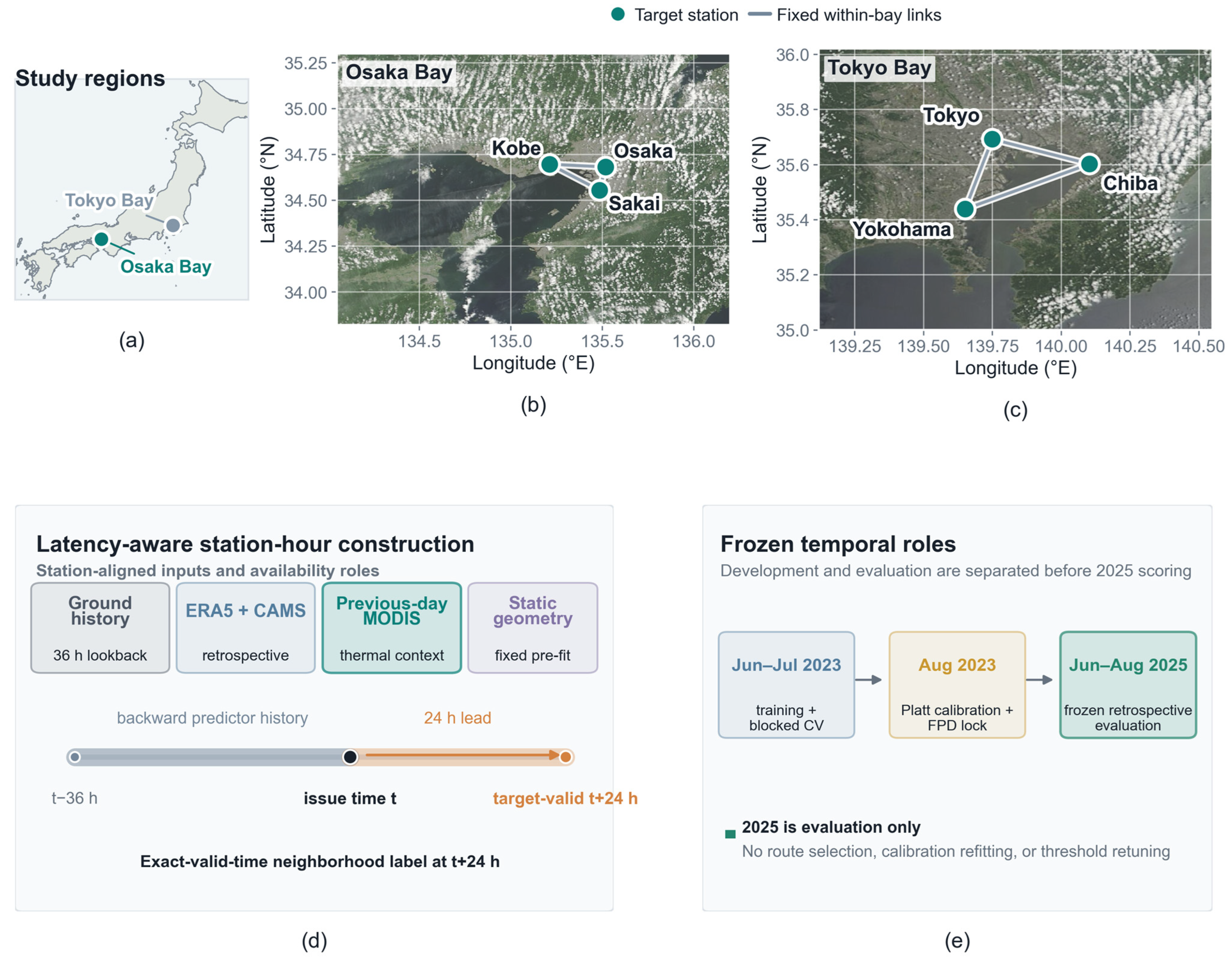
Spatial context and latency-aware analytical design of CoAST-EWS Japan. (a) National locator of the Osaka Bay and Tokyo Bay study regions. (b) Osaka Bay station network comprising Kobe, Osaka, and Sakai, with fixed within-bay links over Earth-observation geographic context. (c) Tokyo Bay station network comprising Tokyo, Yokohama, and Chiba, with the same fixed-link representation. (d) Construction of station-hour samples from a 36 h ground-observation history, retrospective ERA5/CAMS context, previous-day MODIS thermal context, and fixed geometry; the neighborhood label is evaluated at the exact target-valid time, t + 24 h. (e) Frozen temporal roles: June–July 2023 for training and blocked cross-validation, August 2023 for Platt calibration and false-alarm-budget locking, and June–August 2025 for frozen retrospective evaluation. Backgrounds in (b,c) are NASA EOSDIS GIBS Terra/MODIS corrected-reflectance true-color daily composites for 21 July 2025; they provide geographic context only and do not supply quantitative values.
Figure 1.
Spatial context and latency-aware analytical design of CoAST-EWS Japan. (a) National locator of the Osaka Bay and Tokyo Bay study regions. (b) Osaka Bay station network comprising Kobe, Osaka, and Sakai, with fixed within-bay links over Earth-observation geographic context. (c) Tokyo Bay station network comprising Tokyo, Yokohama, and Chiba, with the same fixed-link representation. (d) Construction of station-hour samples from a 36 h ground-observation history, retrospective ERA5/CAMS context, previous-day MODIS thermal context, and fixed geometry; the neighborhood label is evaluated at the exact target-valid time, t + 24 h. (e) Frozen temporal roles: June–July 2023 for training and blocked cross-validation, August 2023 for Platt calibration and false-alarm-budget locking, and June–August 2025 for frozen retrospective evaluation. Backgrounds in (b,c) are NASA EOSDIS GIBS Terra/MODIS corrected-reflectance true-color daily composites for 21 July 2025; they provide geographic context only and do not supply quantitative values.

Figure 2.
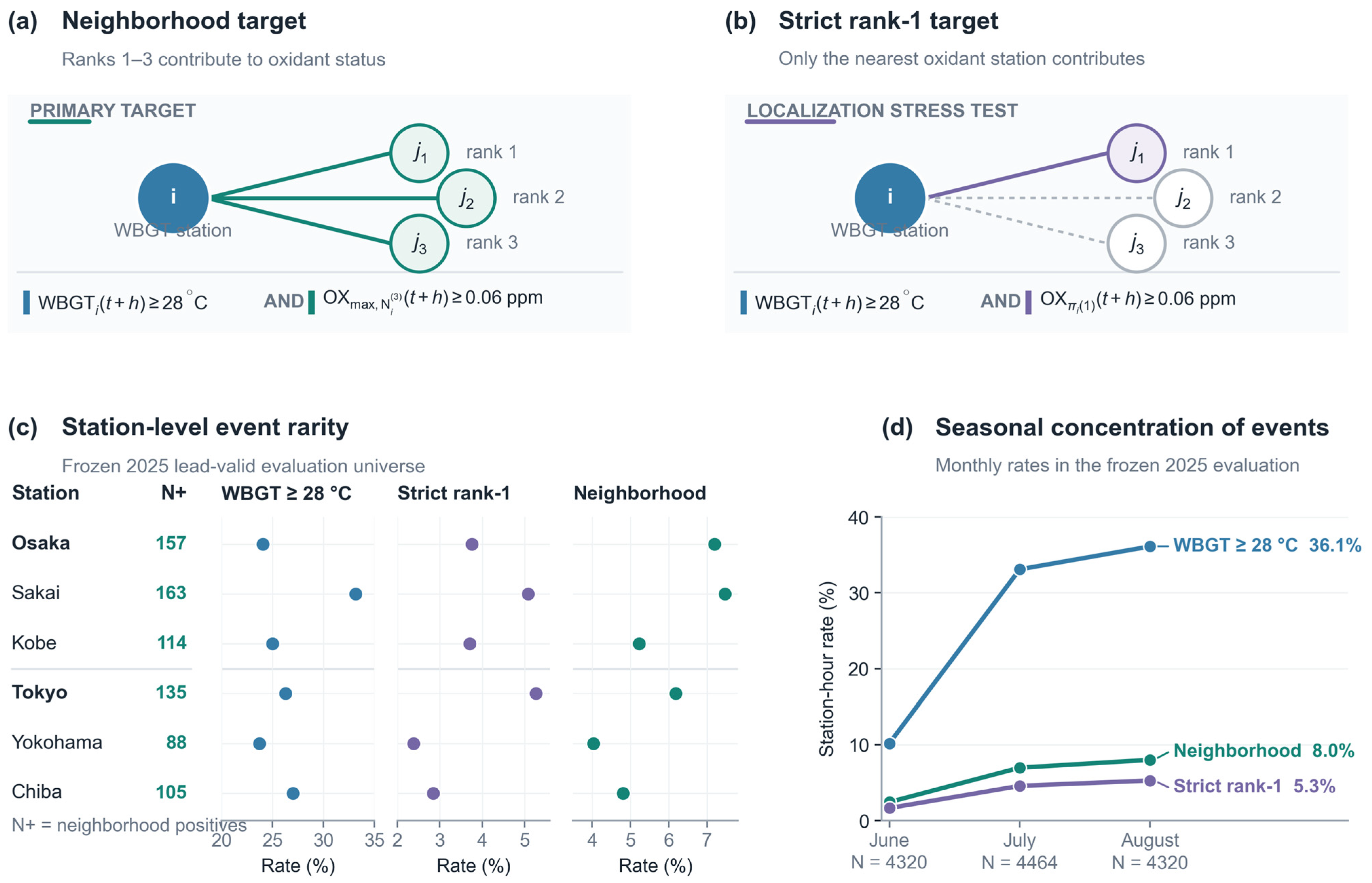
Compound-warning target definitions and event rarity in the frozen 2025 lead-valid evaluation universe. (a) Primary rank-1-to-rank-3 neighborhood target, in which humid-heat exceedance at station i is combined with oxidant exceedance at any of its three fixed nearest oxidant stations. (b) Strict rank-1 localization stress test, in which oxidant exceedance is required at the nearest station only. Colored solid links denote oxidant stations included in each target; gray dashed links are excluded. (c) Station-specific humid-heat, strict rank-1, and neighborhood event rates, with neighborhood positive counts. (d) Monthly station-hour rates from June to August 2025. Rates in panels (c,d) are calculated from the same canonical lead-valid evaluation support used in the corresponding target audit.
Figure 2.
Compound-warning target definitions and event rarity in the frozen 2025 lead-valid evaluation universe. (a) Primary rank-1-to-rank-3 neighborhood target, in which humid-heat exceedance at station i is combined with oxidant exceedance at any of its three fixed nearest oxidant stations. (b) Strict rank-1 localization stress test, in which oxidant exceedance is required at the nearest station only. Colored solid links denote oxidant stations included in each target; gray dashed links are excluded. (c) Station-specific humid-heat, strict rank-1, and neighborhood event rates, with neighborhood positive counts. (d) Monthly station-hour rates from June to August 2025. Rates in panels (c,d) are calculated from the same canonical lead-valid evaluation support used in the corresponding target audit.
Figure 3.
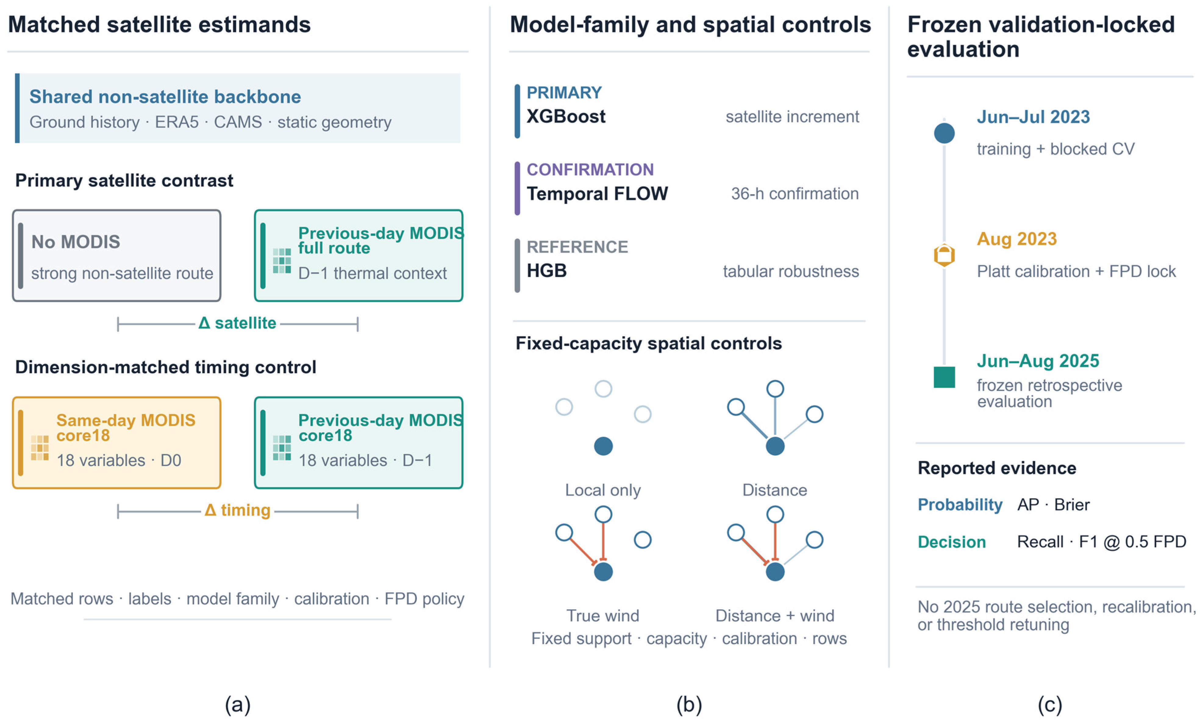
Matched satellite estimands, model-family and spatial controls, and frozen validation-locked evaluation. (a) The primary source contrast compares the no-MODIS route with the previous-day MODIS full route, whereas a separate dimension-matched core18 comparison isolates same-day versus previous-day timing using the same 18 MODIS variables. (b) XGBoost estimates the primary satellite increment, Temporal FLOW provides a 36 h model-family confirmation, HGB serves as a secondary tabular reference, and fixed-capacity spatial controls separate local-only, distance, true-wind, and joint distance–wind context under matched source support. (c) Models are developed using June–July 2023 data, calibrated and threshold-locked on August 2023 predictions, and then applied unchanged to the frozen June–August 2025 retrospective evaluation.
Figure 3.
Matched satellite estimands, model-family and spatial controls, and frozen validation-locked evaluation. (a) The primary source contrast compares the no-MODIS route with the previous-day MODIS full route, whereas a separate dimension-matched core18 comparison isolates same-day versus previous-day timing using the same 18 MODIS variables. (b) XGBoost estimates the primary satellite increment, Temporal FLOW provides a 36 h model-family confirmation, HGB serves as a secondary tabular reference, and fixed-capacity spatial controls separate local-only, distance, true-wind, and joint distance–wind context under matched source support. (c) Models are developed using June–July 2023 data, calibrated and threshold-locked on August 2023 predictions, and then applied unchanged to the frozen June–August 2025 retrospective evaluation.
Figure 4.
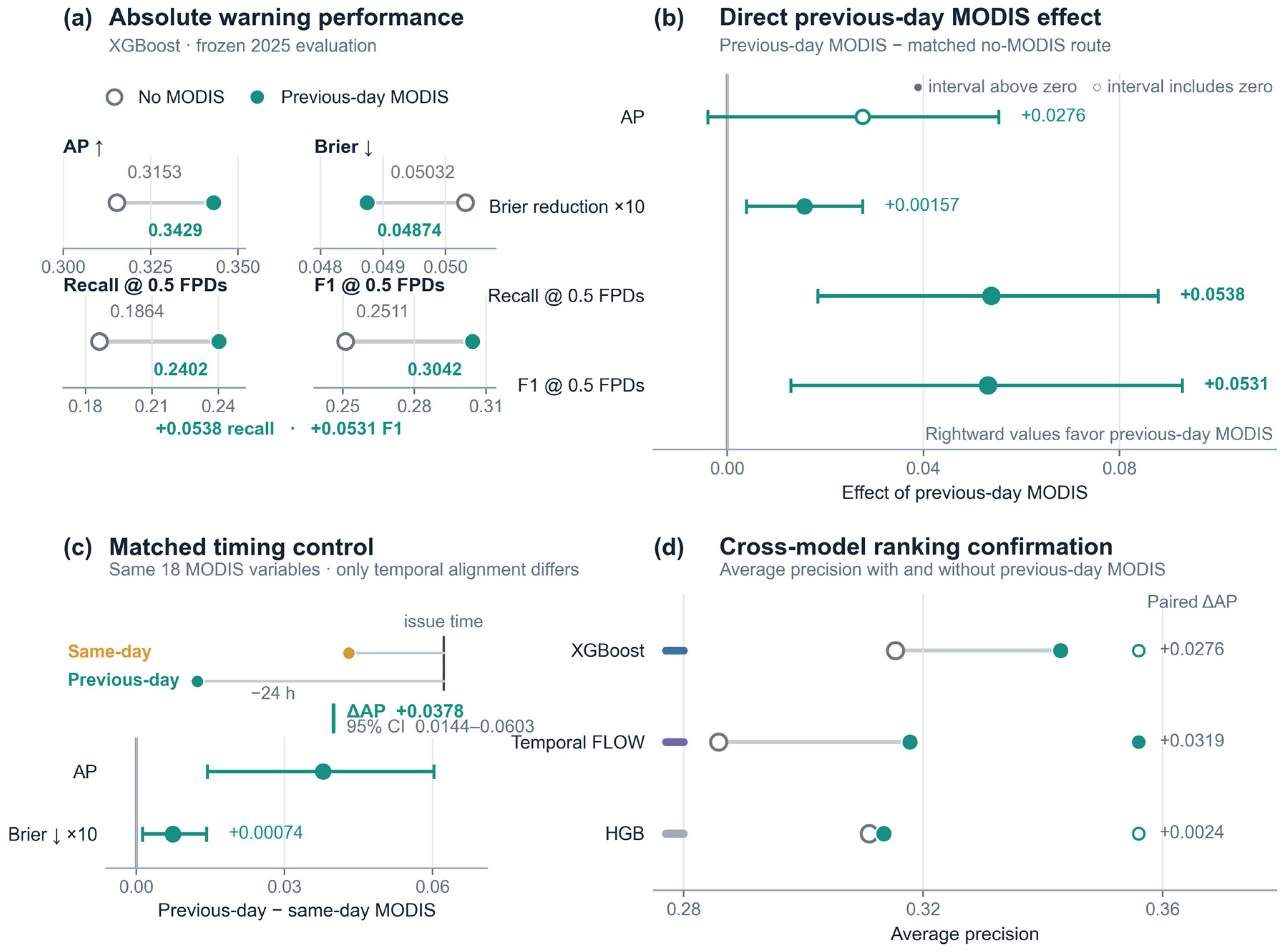
Direct decision value, timing sensitivity, and cross-model confirmation of previous-day MODIS thermal context. (a) Absolute XGBoost probability and decision performance under the validation-locked budget of 0.5 FPDs with and without previous-day MODIS. (b) Paired effects of previous-day MODIS relative to the matched no-MODIS route. Filled markers indicate calendar-day intervals above zero; open markers indicate intervals that include zero. (c) Dimension-matched timing control using the same 18 MODIS variables, model capacity, training protocol, and evaluation rows; only same-day versus previous-day alignment differs. (d) Average-precision changes across XGBoost, Temporal FLOW, and HGB. Error bars in panels (b,c) denote 95% Japan-local calendar-day bootstrap intervals from 10,000 replicates. Brier reductions are multiplied by 10 for display. Upward and downward arrows indicate whether higher or lower values are preferable, respectively.
Figure 4.
Direct decision value, timing sensitivity, and cross-model confirmation of previous-day MODIS thermal context. (a) Absolute XGBoost probability and decision performance under the validation-locked budget of 0.5 FPDs with and without previous-day MODIS. (b) Paired effects of previous-day MODIS relative to the matched no-MODIS route. Filled markers indicate calendar-day intervals above zero; open markers indicate intervals that include zero. (c) Dimension-matched timing control using the same 18 MODIS variables, model capacity, training protocol, and evaluation rows; only same-day versus previous-day alignment differs. (d) Average-precision changes across XGBoost, Temporal FLOW, and HGB. Error bars in panels (b,c) denote 95% Japan-local calendar-day bootstrap intervals from 10,000 replicates. Brier reductions are multiplied by 10 for display. Upward and downward arrows indicate whether higher or lower values are preferable, respectively.
Figure 5.
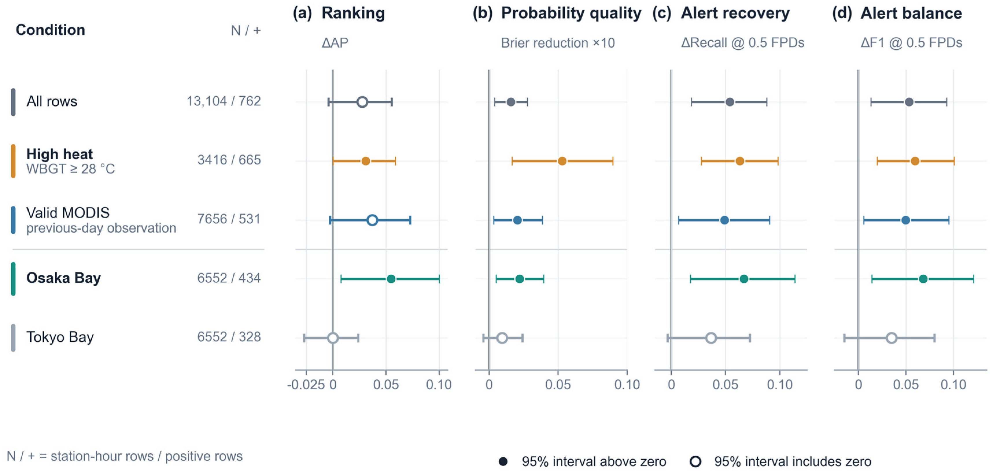
Environmental, source-availability, and geographic concentration of the previous-day MODIS increment. Columns report paired changes in (a) average precision, (b) Brier-score reduction, (c) recall at the validation-locked budget of 0.5 FPDs, and (d) F1 at the same operating point. Rows show the full common evaluation universe, high-heat issue times (WBGT ≥ 28 °C), rows with a valid previous-day MODIS observation, Osaka Bay, and Tokyo Bay. Filled markers indicate 95% Japan-local calendar-day intervals above zero; open markers indicate intervals that include zero. Brier reductions are multiplied by 10 for display. N/+ denotes station-hour rows/positive rows.
Figure 5.
Environmental, source-availability, and geographic concentration of the previous-day MODIS increment. Columns report paired changes in (a) average precision, (b) Brier-score reduction, (c) recall at the validation-locked budget of 0.5 FPDs, and (d) F1 at the same operating point. Rows show the full common evaluation universe, high-heat issue times (WBGT ≥ 28 °C), rows with a valid previous-day MODIS observation, Osaka Bay, and Tokyo Bay. Filled markers indicate 95% Japan-local calendar-day intervals above zero; open markers indicate intervals that include zero. Brier reductions are multiplied by 10 for display. N/+ denotes station-hour rows/positive rows.
Figure 6.
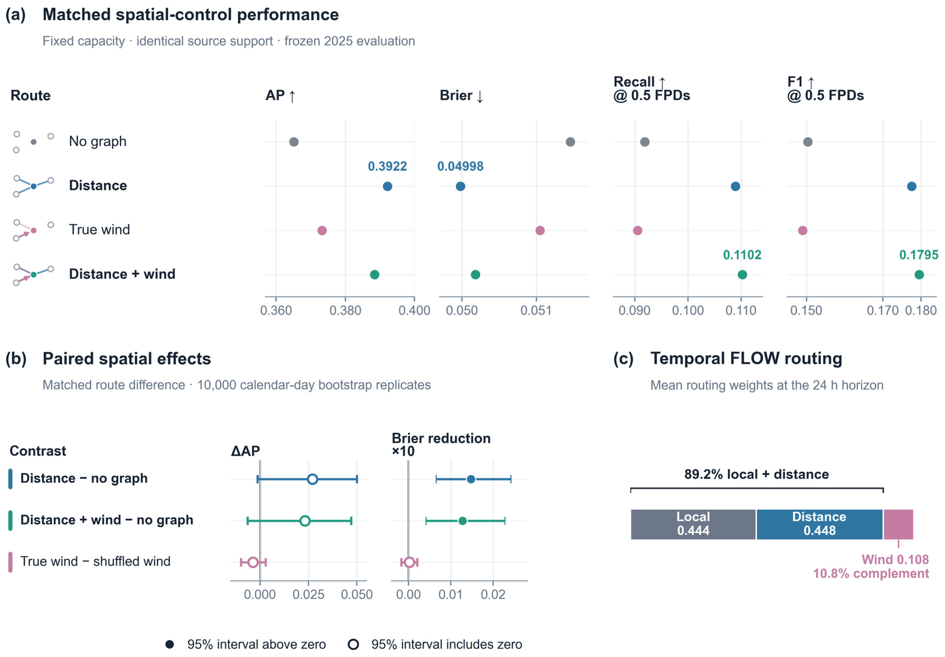
Matched spatial controls and learned routing at the 24 h horizon. (
a) Absolute probability-quality and decision performance under the validation-locked budget of 0.5 FPDs for no-graph, distance, true-wind, and joint distance–wind routes under identical source support and model capacity. (
b) Paired effects for distance and joint routes relative to no graph, and for true wind relative to a spatially shuffled wind control. Filled markers indicate 95% Japan-local calendar-day intervals above zero; open markers indicate intervals that include zero. Brier reductions are multiplied by 10 for display. (
c) Mean local, distance, and wind routing weights learned by the previous-day MODIS Temporal FLOW model. Complete graph-family decision intervals and additional temporal-shuffle, reversed-wind, and edge-permuted controls are reported in
Figure S2 and the Supplementary Materials. Upward and downward arrows indicate whether higher or lower values are preferable, respectively.
Figure 6.
Matched spatial controls and learned routing at the 24 h horizon. (
a) Absolute probability-quality and decision performance under the validation-locked budget of 0.5 FPDs for no-graph, distance, true-wind, and joint distance–wind routes under identical source support and model capacity. (
b) Paired effects for distance and joint routes relative to no graph, and for true wind relative to a spatially shuffled wind control. Filled markers indicate 95% Japan-local calendar-day intervals above zero; open markers indicate intervals that include zero. Brier reductions are multiplied by 10 for display. (
c) Mean local, distance, and wind routing weights learned by the previous-day MODIS Temporal FLOW model. Complete graph-family decision intervals and additional temporal-shuffle, reversed-wind, and edge-permuted controls are reported in
Figure S2 and the Supplementary Materials. Upward and downward arrows indicate whether higher or lower values are preferable, respectively.
Figure 7.
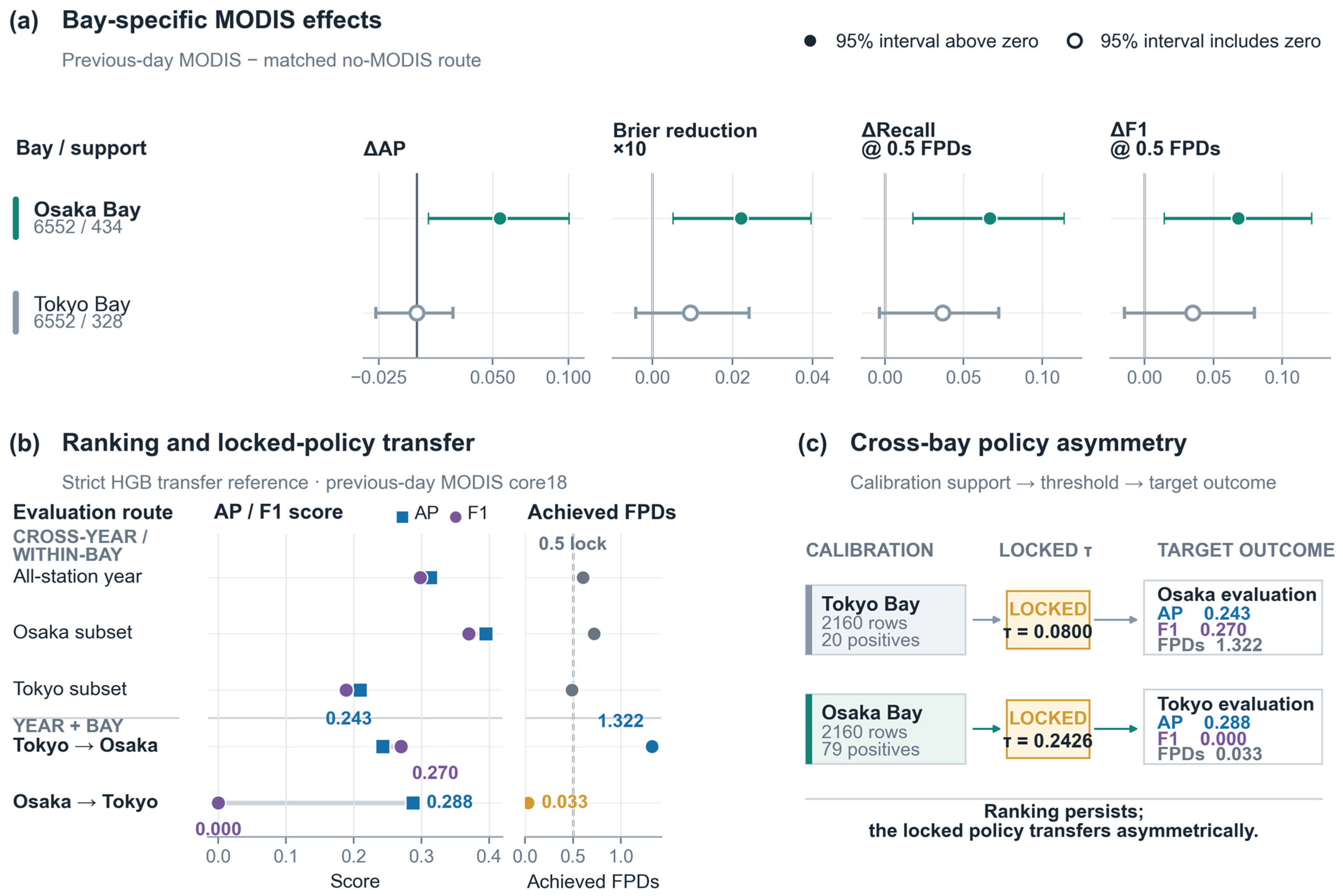
Bay-specific satellite effects and asymmetric transfer of a locked warning policy. (a) Previous-day MODIS increments in Osaka Bay and Tokyo Bay for average precision, Brier-score reduction, recall, and F1 under the validation-locked budget of 0.5 FPDs. Filled markers indicate 95% Japan-local calendar-day intervals above zero; open markers indicate intervals that include zero. Brier reductions are multiplied by 10 for display. (b) HGB average precision, F1, and achieved false alarms per station-day under all-station cross-year evaluation, bay-specific testing, and year-plus-bay transfer. (c) Calibration support, locked thresholds, and target-bay outcomes for the two cross-bay transfer directions. The Tokyo-source and Osaka-source calibration sets contained 20 and 79 positive rows and produced locked thresholds of 0.0800 and 0.2426, respectively. N/+ denotes station-hour rows/positive rows.
Figure 7.
Bay-specific satellite effects and asymmetric transfer of a locked warning policy. (a) Previous-day MODIS increments in Osaka Bay and Tokyo Bay for average precision, Brier-score reduction, recall, and F1 under the validation-locked budget of 0.5 FPDs. Filled markers indicate 95% Japan-local calendar-day intervals above zero; open markers indicate intervals that include zero. Brier reductions are multiplied by 10 for display. (b) HGB average precision, F1, and achieved false alarms per station-day under all-station cross-year evaluation, bay-specific testing, and year-plus-bay transfer. (c) Calibration support, locked thresholds, and target-bay outcomes for the two cross-bay transfer directions. The Tokyo-source and Osaka-source calibration sets contained 20 and 79 positive rows and produced locked thresholds of 0.0800 and 0.2426, respectively. N/+ denotes station-hour rows/positive rows.
Table 1.
Positioning relative to closely related research.
Table 1.
Positioning relative to closely related research.
| Research Stream | Representative Input | Main Task | Spatial/Temporal Method | Primary Evaluation | Gap Addressed Here |
|---|
| Satellite-enhanced air-quality estimation [3,4,5,6,7,8] | TROPOMI, meteorology, land/surface context | Continuous ozone or pollutant estimation | RF, knowledge-informed, and multiscale fusion models | R2, RMSE, MAE, retrieval accuracy | Does not isolate satellite value for locked warning decisions |
| Graph-based and wind-aware air-quality forecasting [9,10] | Monitoring networks, wind, contextual data | Multi-step concentration forecasting or unmonitored-region inference | Dynamic graph attention, Transformer, self-supervised learning | RMSE, MAE, MAPE | Does not compare wind and distance context under compound alert budgets |
| Compound heat–ozone studies [1,2] | Ground/satellite observations and coupled models | Mechanism, co-occurrence, exposure, mitigation | Statistical and meteorology–chemistry analysis | Event frequency, concentration, process attribution | Does not evaluate lead-specific station-hour alert allocation |
| This study | Ground, ERA5, CAMS, MODIS, spatial context | 24 h compound warning | Boosted trees and Temporal/Spatial FLOW controls | AP, Brier, validation-locked FPDs | Quantifies when latency-aware satellite context changes warning decisions |
Table 2.
Exact temporal roles and support for the primary 24 h task.
Table 2.
Exact temporal roles and support for the primary 24 h task.
| Role | Issue-Time Range | Target-Valid Range | Stations | Support | Positives | Analytical Role |
|---|
| Model fitting | 1 June–30 July 2023 | 2 June–31 July 2023 | 6 | 8640 lead-valid; 8430 XGBoost-evaluable | 286 | Parameter fitting and blocked-CV development |
| Calibration and threshold locking | 1–30 August 2023 | 2–31 August 2023 | 6 | 4320 lead-valid; 4320 XGBoost-evaluable | 99 | Platt calibration and FPDs threshold selection |
| Retrospective cross-year evaluation | 1 June–30 August 2025 | 2 June–31 August 2025 | 6 | 13,104 lead-valid; 13,104 XGBoost-evaluable | 762 | Frozen cross-year evaluation |
Table 3.
Matched source routes used to estimate MODIS contribution.
Table 3.
Matched source routes used to estimate MODIS contribution.
| Route | Ground | ERA5 | CAMS | Geometry | MODIS Timing | Purpose |
|---|
| No-MODIS baseline | Included | Included | Included | Included | None | Strong non-satellite baseline |
| Previous-day MODIS | Included | Included | Included | Included | Previous local day | Primary satellite increment |
| Same-day MODIS core18 | Included | Included | Included | Included | Same local day | Matched timing comparator |
| Previous-day MODIS core18 | Included | Included | Included | Included | Previous local day | Matched timing comparator |
Table 4.
Warning value of previous-day MODIS on the frozen 2025 cross-year evaluation.
Table 4.
Warning value of previous-day MODIS on the frozen 2025 cross-year evaluation.
| Route or Statistic | AP | Brier | Recall @ 0.5 FPDs | F1 @ 0.5 FPDs |
|---|
| No-MODIS XGBoost | 0.3153 | 0.05032 | 0.1864 | 0.2511 |
| Previous-day MODIS XGBoost | 0.3429 | 0.04874 | 0.2402 | 0.3042 |
| Previous-day MODIS effect | +0.0276 | +0.00157 reduction | +0.0538 | +0.0531 |
| 95% calendar-day CI | [−0.0040, +0.0554] | [+0.00039, +0.00276] | [+0.0184, +0.0879] | [+0.0129, +0.0928] |
Table 5.
Dimension-matched comparison of same-day and previous-day MODIS timing.
Table 5.
Dimension-matched comparison of same-day and previous-day MODIS timing.
| MODIS Timing Route | MODIS Variables | AP | Brier |
|---|
| Same-day MODIS core18 | 18 | 0.3260 | 0.05141 |
| Previous-day MODIS core18 | 18 | 0.3638 | 0.05067 |
| Previous-day—Same-day | — | +0.0378 | +0.000742 reduction |
| 95% calendar-day CI | — | [0.0144, 0.0603] | [0.000131, 0.001422] |
Table 6.
Environmental and geographic concentration of the previous-day MODIS increment.
Table 6.
Environmental and geographic concentration of the previous-day MODIS increment.
| Stratum | Rows | Positive Rows | ΔAP | Brier Reduction | ΔRecall at 0.5 FPDs | ΔF1 at 0.5 FPDs |
|---|
| All rows | 13,104 | 762 | +0.0276 | +0.00157 | +0.0538 | +0.0531 |
| High heat, WBGT ≥ 28 °C | 3416 | 665 | +0.0310 | +0.00528 | +0.0632 | +0.0595 |
| Osaka Bay | 6552 | 434 | +0.0548 | +0.00221 | +0.0668 | +0.0680 |
Table 7.
Fixed-capacity spatial controls on the 24 h neighborhood task.
Table 7.
Fixed-capacity spatial controls on the 24 h neighborhood task.
| Spatial Route | AP | Brier | Recall at 0.5 FPDs | F1 at 0.5 FPDs |
|---|
| No graph | 0.3652 | 0.05145 | 0.0919 | 0.1504 |
| Distance graph | 0.3922 | 0.04998 | 0.1089 | 0.1775 |
| True-wind graph | 0.3733 | 0.05105 | 0.0906 | 0.1490 |
| Joint distance–wind | 0.3884 | 0.05018 | 0.1102 | 0.1795 |