Author Contributions
Conceptualization, Y.L. and J.H.; methodology, Y.L.; software, Y.L.; validation, Y.L. and H.Z.; formal analysis, Y.L. and Y.Y.; investigation, Y.L., Y.W. and Y.Z.; resources, J.H.; data curation, Y.L.; writing—original draft preparation, Y.L.; writing—review and editing, J.H., Y.W., Y.Z., Y.Y. and H.Z.; visualization, Y.L.; supervision, J.H. All authors have read and agreed to the published version of the manuscript.
Figure 1.
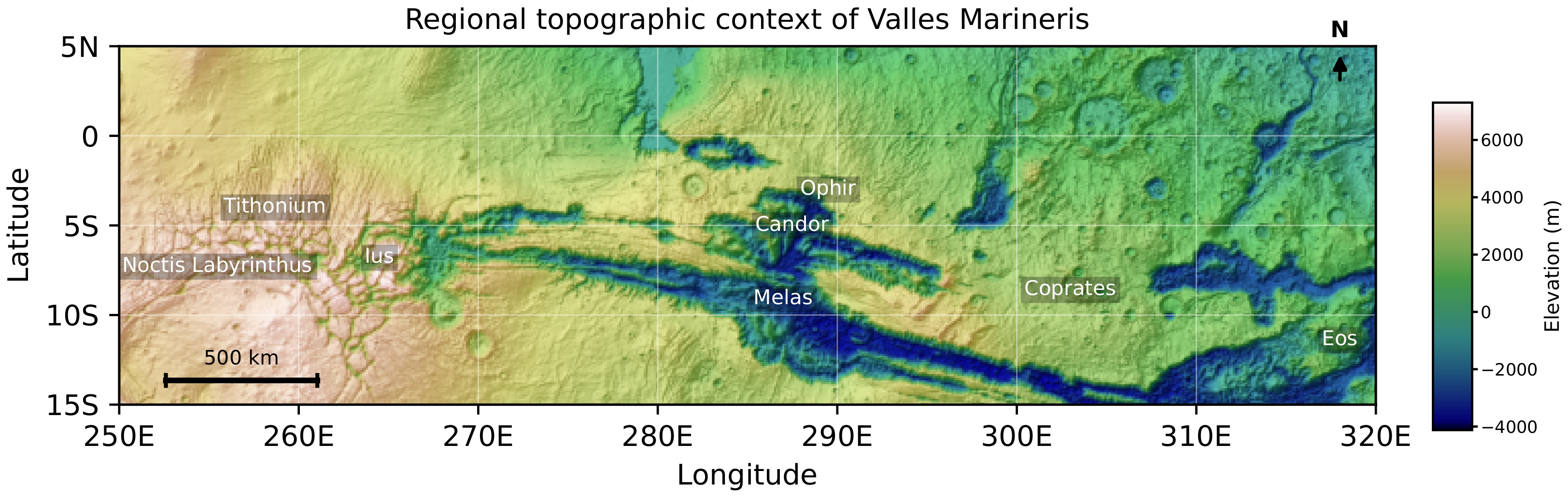
Regional topographic context of Valles Marineris used to introduce the geomorphic setting of Martian landslide segmentation. The map shows MGS MOLA shaded relief and elevation for the study region, with major canyon-system place names, a scale bar, a north arrow, and an elevation color bar. No landslide labels, candidate points, or dataset display panels are shown in this figure; it is used only as a regional geomorphic context map.
Figure 1.
Regional topographic context of Valles Marineris used to introduce the geomorphic setting of Martian landslide segmentation. The map shows MGS MOLA shaded relief and elevation for the study region, with major canyon-system place names, a scale bar, a north arrow, and an elevation color bar. No landslide labels, candidate points, or dataset display panels are shown in this figure; it is used only as a regional geomorphic context map.
Figure 2.
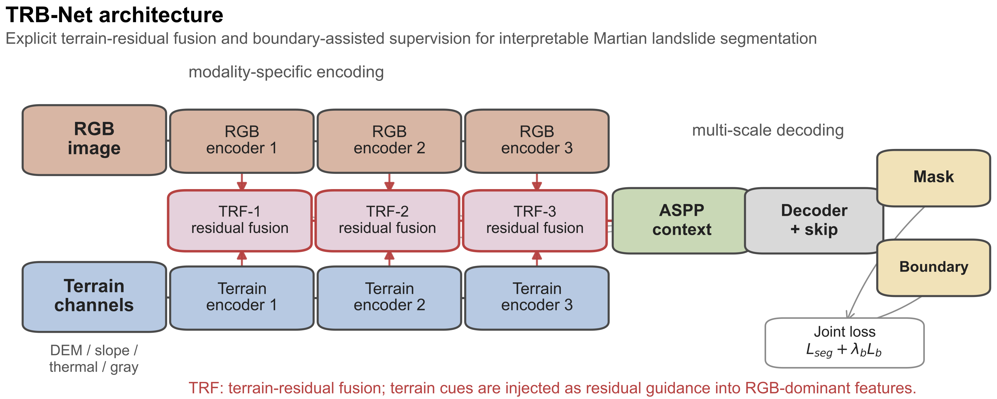
Conceptual overview of the TRB-Net design. Brown blocks denote the RGB pathway, blue blocks denote the terrain-thermophysical pathway, red blocks denote terrain-residual fusion (TRF), the green block denotes ASPP context aggregation, the gray block denotes the decoder and skip connections, and yellow blocks denote the mask and boundary outputs. Horizontal lines indicate forward feature propagation, vertical red arrows indicate injection of terrain guidance into RGB-dominant features, and the two output branches contribute to the joint loss. The multiscale implementation used for component ablations applies TRF at four encoder scales; the compact evaluation implementation applies the same residual-fusion principle at the low-level stem before an ASPP decoder.
Figure 2.
Conceptual overview of the TRB-Net design. Brown blocks denote the RGB pathway, blue blocks denote the terrain-thermophysical pathway, red blocks denote terrain-residual fusion (TRF), the green block denotes ASPP context aggregation, the gray block denotes the decoder and skip connections, and yellow blocks denote the mask and boundary outputs. Horizontal lines indicate forward feature propagation, vertical red arrows indicate injection of terrain guidance into RGB-dominant features, and the two output branches contribute to the joint loss. The multiscale implementation used for component ablations applies TRF at four encoder scales; the compact evaluation implementation applies the same residual-fusion principle at the low-level stem before an ASPP decoder.
Figure 3.
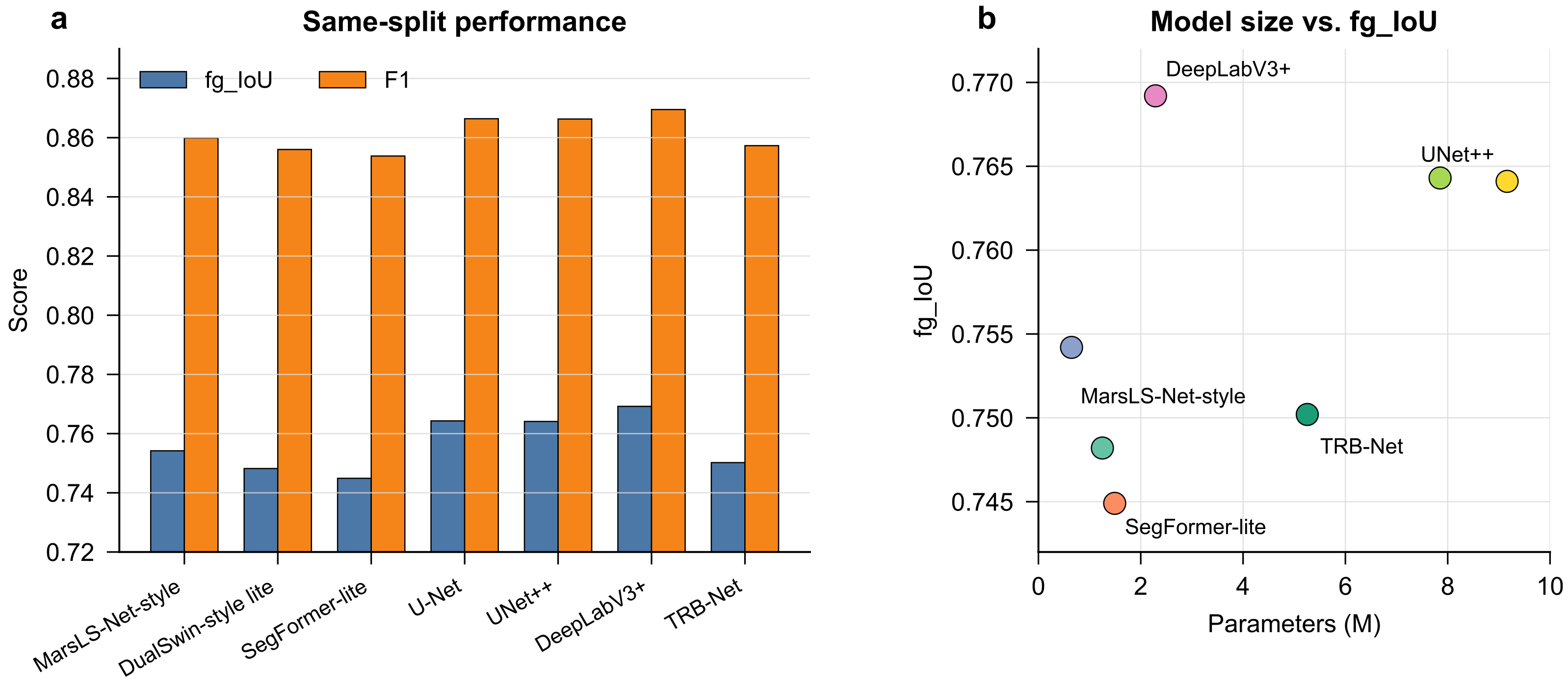
Same-split comparison on the local MMLSv2 test split. (a) Test foreground IoU and F1-score of TRB-Net-Compact and baseline models. (b) Model size versus test foreground IoU, where parameter count is used only as a complexity indicator; the purple point denotes DeepLabV3+.
Figure 3.
Same-split comparison on the local MMLSv2 test split. (a) Test foreground IoU and F1-score of TRB-Net-Compact and baseline models. (b) Model size versus test foreground IoU, where parameter count is used only as a complexity indicator; the purple point denotes DeepLabV3+.
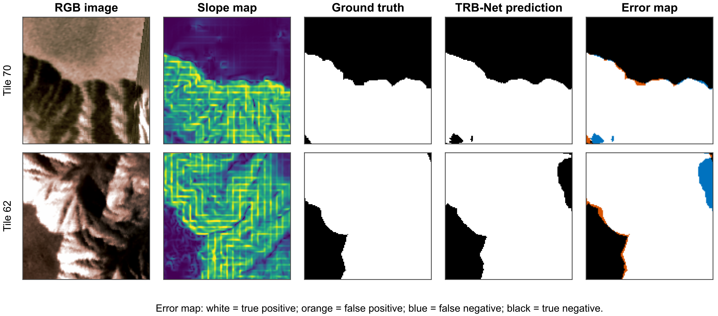
Figure 4.
Manually selected illustrative local MMLSv2 test cases, part 1: tile 70 (sample col00039_row00001) and tile 62 (sample col00035_row00018). From left to right, each row shows the RGB image, slope map, ground-truth mask, TRB-Net-Compact prediction, and pixel-level error map. Slope maps use a purple-to-yellow scale from lower to higher slope values. White, orange, blue, and black denote true positives, false positives, false negatives, and true negatives, respectively. These examples were selected to display mask-extent and boundary-error variation rather than by a random or best-score rule.
Figure 4.
Manually selected illustrative local MMLSv2 test cases, part 1: tile 70 (sample col00039_row00001) and tile 62 (sample col00035_row00018). From left to right, each row shows the RGB image, slope map, ground-truth mask, TRB-Net-Compact prediction, and pixel-level error map. Slope maps use a purple-to-yellow scale from lower to higher slope values. White, orange, blue, and black denote true positives, false positives, false negatives, and true negatives, respectively. These examples were selected to display mask-extent and boundary-error variation rather than by a random or best-score rule.
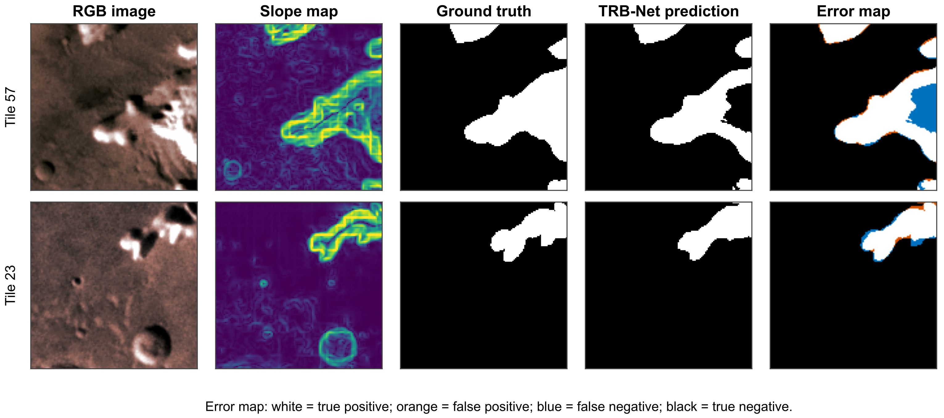
Figure 5.
Additional manually selected illustrative local MMLSv2 test cases, part 2: tile 57 (sample
col00027_row00014) and tile 23 (sample
col00013_row00012). The panel order, color convention, and selection purpose are the same as in
Figure 4.
Figure 5.
Additional manually selected illustrative local MMLSv2 test cases, part 2: tile 57 (sample
col00027_row00014) and tile 23 (sample
col00013_row00012). The panel order, color convention, and selection purpose are the same as in
Figure 4.
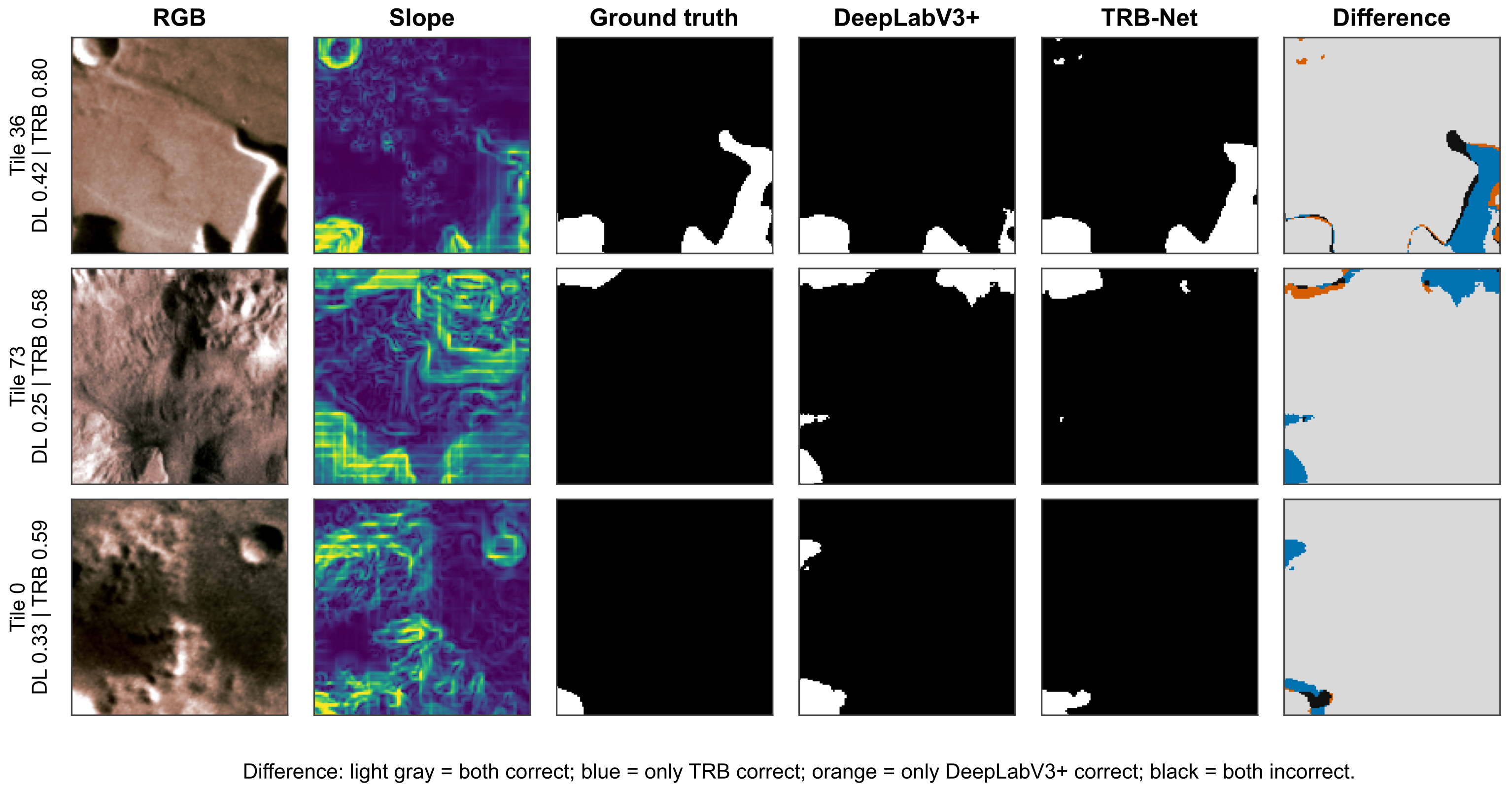
Figure 6.
Purposefully selected favorable-case comparison between DeepLabV3+ and TRB-Net-Compact. The three rows are the test tiles with the largest positive TRB-Net-minus-DeepLabV3+ foreground-IoU differences (tiles 36, 73, and 0). Slope maps use purple for lower and yellow for higher values. In the ground-truth and prediction masks, white denotes foreground and black denotes background. In the difference map, blue denotes pixels correctly classified only by TRB-Net-Compact, orange denotes pixels correctly classified only by DeepLabV3+, light gray denotes pixels correctly classified by both, and black denotes pixels misclassified by both. This figure is diagnostic and does not represent aggregate superiority.
Figure 6.
Purposefully selected favorable-case comparison between DeepLabV3+ and TRB-Net-Compact. The three rows are the test tiles with the largest positive TRB-Net-minus-DeepLabV3+ foreground-IoU differences (tiles 36, 73, and 0). Slope maps use purple for lower and yellow for higher values. In the ground-truth and prediction masks, white denotes foreground and black denotes background. In the difference map, blue denotes pixels correctly classified only by TRB-Net-Compact, orange denotes pixels correctly classified only by DeepLabV3+, light gray denotes pixels correctly classified by both, and black denotes pixels misclassified by both. This figure is diagnostic and does not represent aggregate superiority.
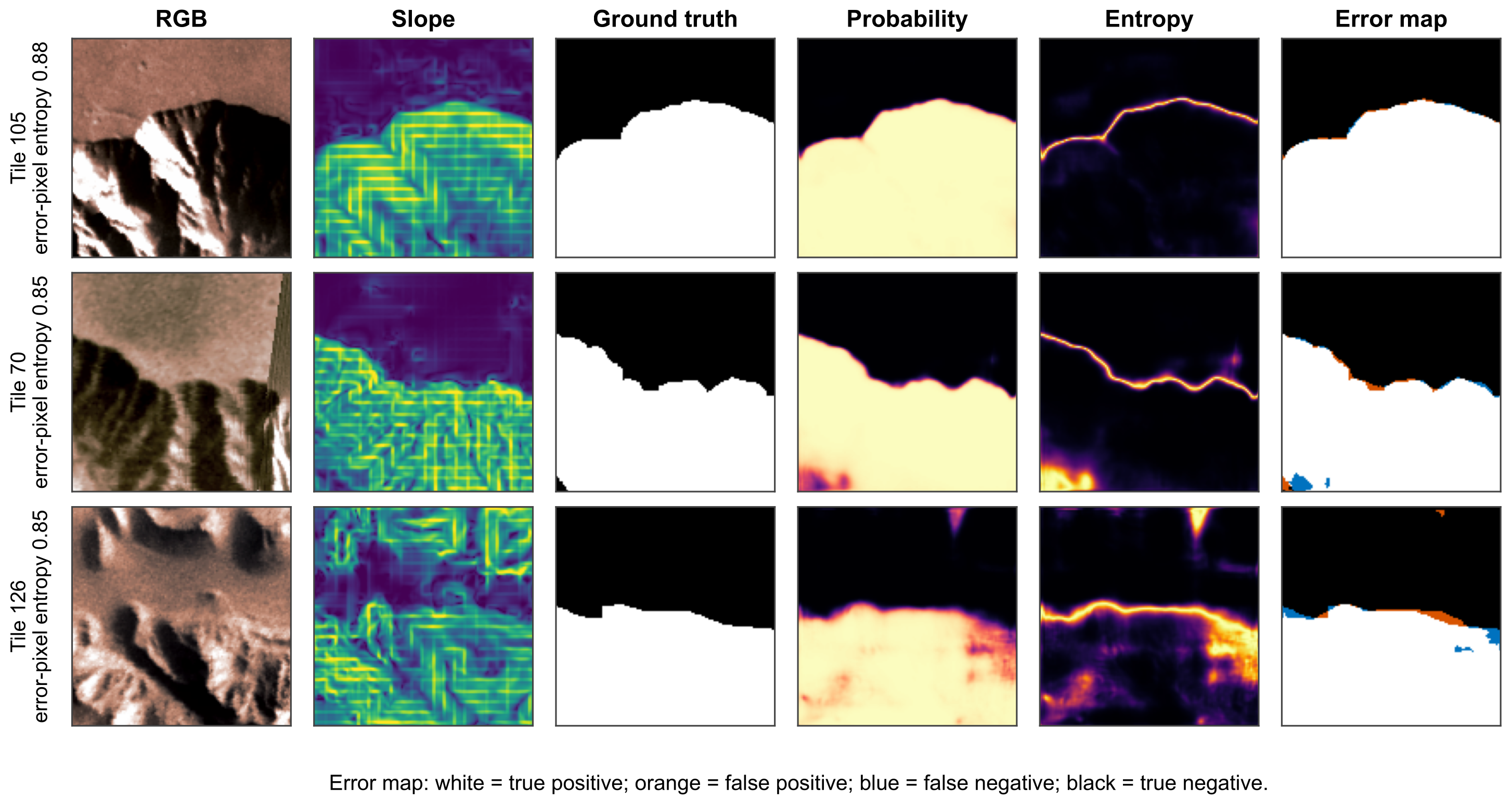
Figure 7.
Probability, uncertainty, and error analysis of TRB-Net-Compact on three purposefully selected local MMLSv2 test tiles (tiles 105, 70, and 126). These tiles have the highest mean predictive entropy over their misclassified pixels and therefore illustrate difficult cases rather than a random sample. Slope maps use purple for lower and yellow for higher values; probability and entropy maps use dark colors for lower and bright yellow/white for higher values. The probability map shows foreground probability, and the uncertainty map is binary predictive entropy, . Error maps use white for true positives, orange for false positives, blue for false negatives, and black for true negatives.
Figure 7.
Probability, uncertainty, and error analysis of TRB-Net-Compact on three purposefully selected local MMLSv2 test tiles (tiles 105, 70, and 126). These tiles have the highest mean predictive entropy over their misclassified pixels and therefore illustrate difficult cases rather than a random sample. Slope maps use purple for lower and yellow for higher values; probability and entropy maps use dark colors for lower and bright yellow/white for higher values. The probability map shows foreground probability, and the uncertainty map is binary predictive entropy, . Error maps use white for true positives, orange for false positives, blue for false negatives, and black for true negatives.
Figure 8.
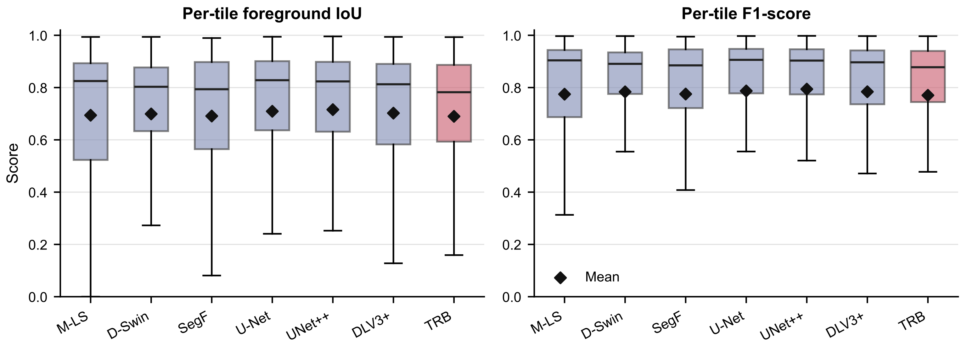
Per-tile performance distribution on the local MMLSv2 test split. Box plots report sample-level foreground IoU and F1-score across the 133 test tiles; boxes indicate the interquartile range, center lines indicate medians, whiskers indicate the non-outlier range, and black diamonds denote mean values. The broad interquartile ranges indicate that local MMLSv2 performance is strongly affected by tile-level heterogeneity rather than by average model score alone. Model names are abbreviated on the horizontal axis for readability.
Figure 8.
Per-tile performance distribution on the local MMLSv2 test split. Box plots report sample-level foreground IoU and F1-score across the 133 test tiles; boxes indicate the interquartile range, center lines indicate medians, whiskers indicate the non-outlier range, and black diamonds denote mean values. The broad interquartile ranges indicate that local MMLSv2 performance is strongly affected by tile-level heterogeneity rather than by average model score alone. Model names are abbreviated on the horizontal axis for readability.
Figure 9.
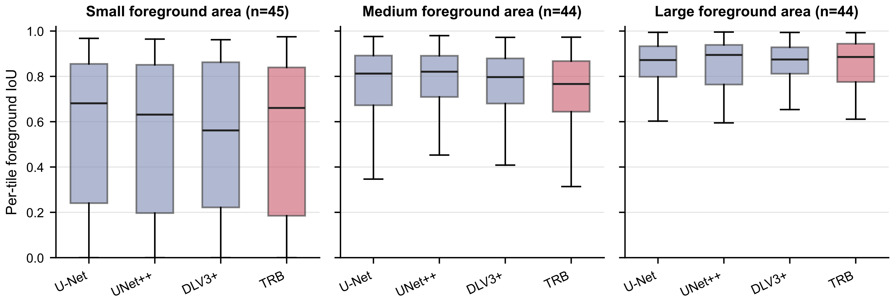
Size-stratified per-tile foreground IoU for representative strong baselines and TRB-Net-Compact on the local MMLSv2 test split. Test tiles are divided by the tertiles of the ground-truth foreground ratio: small, (); medium, (); and large, (). Model names are abbreviated on the horizontal axis for readability.
Figure 9.
Size-stratified per-tile foreground IoU for representative strong baselines and TRB-Net-Compact on the local MMLSv2 test split. Test tiles are divided by the tertiles of the ground-truth foreground ratio: small, (); medium, (); and large, (). Model names are abbreviated on the horizontal axis for readability.
Figure 10.
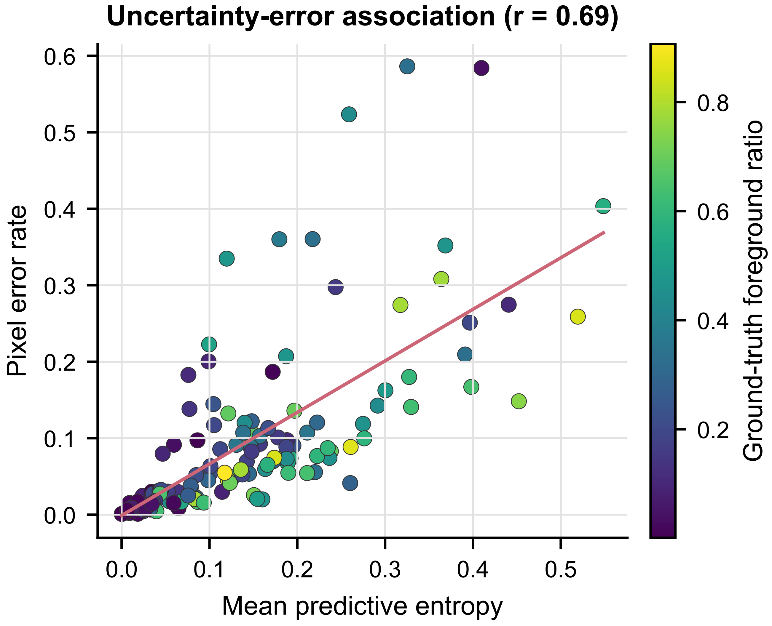
Relationship between mean predictive uncertainty and pixel error rate for TRB-Net-Compact on the local MMLSv2 test split. Each point represents one test tile, mean uncertainty is computed from binary predictive entropy, and point color denotes the ground-truth foreground ratio. The pink line is the ordinary least-squares linear regression trend.
Figure 10.
Relationship between mean predictive uncertainty and pixel error rate for TRB-Net-Compact on the local MMLSv2 test split. Each point represents one test tile, mean uncertainty is computed from binary predictive entropy, and point color denotes the ground-truth foreground ratio. The pink line is the ordinary least-squares linear regression trend.
Table 1.
Dataset used in this study [
6].
Table 1.
Dataset used in this study [
6].
| Dataset | Task | Modalities/Channels | Patch Size | Split Used in This Study |
|---|
| MMLSv2 | Martian landslide semantic segmentation | RGB, DEM, slope, thermal inertia, and grayscale;
seven channels | | Provided local split: train 465/validation 66/test 133; isolated-test folder
unavailable locally |
Table 2.
Experimental settings for the two explicitly distinguished TRB-Net implementations.
Table 2.
Experimental settings for the two explicitly distinguished TRB-Net implementations.
| Parameter | TRB-Net-Compact | TRB-Net-Multiscale |
|---|
| Role in manuscript | Main comparison | Component ablations |
| Input size | | |
| Base channels | 48 | 32 |
| Parameters | 5.255 M | 6.952 M |
| Epochs/batch size | 220/4 | 220/4 |
| Optimizer | AdamW | AdamW |
| Learning rate/weight decay | / | / |
| Scheduler | Cosine annealing | Cosine annealing |
| Segmentation loss | weighted BCE + Dice loss | CE + Dice loss + focal loss |
| Boundary-loss weight | 0.10 | 0.50 |
| Validation-selected threshold | 0.55 | 0.65 |
| Device/mixed precision | RTX 5060 Laptop GPU/enabled | RTX 5060 Laptop GPU/enabled |
Table 3.
Quantitative results of TRB-Net-Compact on the local MMLSv2 test split.
Table 3.
Quantitative results of TRB-Net-Compact on the local MMLSv2 test split.
| Metric | Value |
|---|
| Loss | 0.4883 |
| Accuracy | 0.9023 |
| mIoU | 0.8060 |
| Foreground IoU | 0.7502 |
| F1-score | 0.8573 |
| Precision | 0.8473 |
| Recall | 0.8676 |
| Threshold | 0.55 |
| Parameters | 5.255 M |
Table 4.
Same-split comparison on the local MMLSv2 test split. “Style” and “lite” models are local architectural approximations or lightweight implementations and are not official implementations from the cited authors.
Table 4.
Same-split comparison on the local MMLSv2 test split. “Style” and “lite” models are local architectural approximations or lightweight implementations and are not official implementations from the cited authors.
| Model | Dataset/Split | Parameters (M) | mIoU | Foreground IoU | F1-Score | Precision | Recall |
|---|
| MarsLS-Net-style | MMLSv2 local test | 0.647 | 0.8093 | 0.7542 | 0.8599 | 0.8512 | 0.8688 |
| DualSwin-style lite | MMLSv2 local test | 1.250 | 0.8047 | 0.7482 | 0.8560 | 0.8484 | 0.8637 |
| SegFormer-lite | MMLSv2 local test | 1.491 | 0.8002 | 0.7449 | 0.8538 | 0.8311 | 0.8778 |
| U-Net | MMLSv2 local test | 7.851 | 0.8178 | 0.7643 | 0.8664 | 0.8622 | 0.8706 |
| UNet++ | MMLSv2 local test | 9.161 | 0.8174 | 0.7641 | 0.8663 | 0.8605 | 0.8721 |
| DeepLabV3+ | MMLSv2 local test | 2.289 | 0.8216 | 0.7692 | 0.8695 | 0.8653 | 0.8738 |
| TRB-Net-Compact | MMLSv2 local test | 5.255 | 0.8060 | 0.7502 | 0.8573 | 0.8473 | 0.8676 |
Table 5.
Reported overlap scores and explicit architecture attributes; the last three columns are design descriptors, not measured interpretability scores.
Table 5.
Reported overlap scores and explicit architecture attributes; the last three columns are design descriptors, not measured interpretability scores.
| Model | mIoU | Foreground IoU | F1-Score | Parameters (M) | Separate Terrain Branch | Residual Terrain Fusion | Boundary Auxiliary Loss |
|---|
| DeepLabV3+ | 0.8216 | 0.7692 | 0.8695 | 2.289 | No | No | No |
| TRB-Net-Compact | 0.8060 | 0.7502 | 0.8573 | 5.255 | Yes | Yes | Yes |
Table 6.
Three-seed stability comparison on the local MMLSv2 test split. Values are mean ± standard deviation; each model used the same validation-selected threshold for all three seeds.
Table 6.
Three-seed stability comparison on the local MMLSv2 test split. Values are mean ± standard deviation; each model used the same validation-selected threshold for all three seeds.
| Model | Seeds | mIoU | Foreground IoU | F1-Score | Precision | Recall | Threshold |
|---|
| DeepLabV3+ | 3 | 0.8173 ± 0.0045 | 0.7628 ± 0.0060 | 0.8654 ± 0.0039 | 0.8688 ± 0.0090 | 0.8621 ± 0.0114 | 0.60 |
| TRB-Net-Compact | 3 | 0.8116 ± 0.0056 | 0.7559 ± 0.0057 | 0.8610 ± 0.0037 | 0.8607 ± 0.0136 | 0.8614 ± 0.0063 | 0.55 |
Table 7.
Modality ablation results.
Table 7.
Modality ablation results.
| Variant | Input Channels | mIoU | Foreground IoU | F1-Score | Precision | Recall | Threshold |
|---|
| Multiscale reference | RGB + DEM + thermal inertia + slope + grayscale | 0.8021 | 0.7473 | 0.8554 | 0.8326 | 0.8795 | 0.65 |
| RGB only | RGB | 0.6964 | 0.6170 | 0.7632 | 0.7428 | 0.7847 | 0.55 |
| Terrain only | DEM + thermal inertia + slope + grayscale | 0.1694 | 0.3381 | 0.5054 | 0.3382 | 0.9992 | 0.40 |
Table 8.
Single-channel removal ablation results.
Table 8.
Single-channel removal ablation results.
| Variant | Removed Channel | mIoU | Foreground IoU | F1-Score | Precision | Recall | Threshold |
|---|
| Multiscale reference | None | 0.8021 | 0.7473 | 0.8554 | 0.8326 | 0.8795 | 0.65 |
| Without DEM | DEM | 0.8071 | 0.7514 | 0.8580 | 0.8498 | 0.8665 | 0.45 |
| Without slope | slope | 0.7964 | 0.7382 | 0.8494 | 0.8396 | 0.8595 | 0.70 |
| Without thermal inertia | thermal inertia | 0.7915 | 0.7338 | 0.8465 | 0.8262 | 0.8678 | 0.55 |
| Without grayscale | grayscale | 0.7687 | 0.6998 | 0.8234 | 0.8347 | 0.8124 | 0.60 |
Table 9.
Fusion-strategy ablation.
Table 9.
Fusion-strategy ablation.
| Variant | Fusion Strategy | mIoU | Foreground IoU | F1-Score | Precision | Recall | Threshold |
|---|
| Simple concatenation | | 0.7845 | 0.7249 | 0.8405 | 0.8212 | 0.8607 | 0.50 |
| Sum fusion | | 0.7919 | 0.7334 | 0.8462 | 0.8308 | 0.8622 | 0.55 |
| Weighted sum | | 0.7818 | 0.7204 | 0.8375 | 0.8248 | 0.8505 | 0.55 |
| Attention fusion | | 0.7829 | 0.7182 | 0.8360 | 0.8455 | 0.8266 | 0.60 |
| Terrain-residual fusion | | 0.8021 | 0.7473 | 0.8554 | 0.8326 | 0.8795 | 0.65 |
Table 10.
ASPP ablation.
| Variant | ASPP Module | mIoU | Foreground IoU | F1-Score | Precision | Recall | Threshold |
|---|
| Without ASPP | No | 0.7764 | 0.7123 | 0.8320 | 0.8272 | 0.8368 | 0.55 |
| Multiscale reference | Yes | 0.8021 | 0.7473 | 0.8554 | 0.8326 | 0.8795 | 0.65 |
Table 11.
Performance of TRB-Net-Multiscale at the validation-selected threshold of 0.65.
Table 11.
Performance of TRB-Net-Multiscale at the validation-selected threshold of 0.65.
| Dataset | Threshold | Accuracy | mIoU | Foreground IoU | F1-Score | Precision | Recall |
|---|
| Validation | 0.65 | 0.9027 | 0.8046 | 0.7453 | 0.8541 | 0.8100 | 0.9032 |
| Test | 0.65 | 0.8994 | 0.8021 | 0.7473 | 0.8554 | 0.8326 | 0.8795 |
Table 12.
Boundary supervision ablation results.
Table 12.
Boundary supervision ablation results.
| Variant | Boundary Weight | mIoU | Foreground IoU | F1-Score | Precision | Recall | Threshold |
|---|
| Multiscale reference | 0.50 | 0.8021 | 0.7473 | 0.8554 | 0.8326 | 0.8795 | 0.65 |
| Without boundary supervision | 0.00 | 0.7955 | 0.7352 | 0.8474 | 0.8492 | 0.8457 | 0.65 |
Table 13.
Boundary-sensitive diagnostic metrics for boundary supervision ablation.
Table 13.
Boundary-sensitive diagnostic metrics for boundary supervision ablation.
| Variant | Boundary F1 | Boundary IoU |
|---|
| Multiscale reference | 0.5236 | 0.3234 |
| Without boundary supervision | 0.5147 | 0.3168 |