Assessing the Impact of Spatial Resolution and Aggregation Method on Sentinel-2 NDVI Time Series in Grasslands of Mainland Spain

Highlights

What are the main findings?

• Sentinel-2 at 10 m and 20 m preserves NDVI temporal consistency in grasslands, while 60 m causes substantial degradation and excludes over half of the plots under pure-pixel sampling. Formal Kruskal–Wallis testing and Cliff’s Delta effect-size analysis confirm that spatial resolution—not the aggregation method—is the dominant factor governing time series fidelity.
• Parcel area and Köppen climate class are key modulators: the smallest plots (<3 ha) exhibit large effect sizes (${\epsilon }^2=0.273$), while climate decisively shapes phenological trajectories (up to ${\epsilon }^2=0.447$), with spatial degradation distorting the temporal signal unequally across climate classes.
• The pixel-selection strategy (pure-pixel vs. centroid) has minimal impact at 10 m and 20 m but becomes relevant at 60 m, where pure-pixel sampling slightly improves NDVI reliability.

What are the implications of the main findings?

• A multi-scale Sentinel-2 strategy is supported: 10 m resolution for fragmented, heterogeneous grasslands (<3 ha) typical of humid regions, and 20 m as a computationally efficient alternative (78% storage reduction, 72% faster processing) for large, homogeneous plots (>10 ha) in Mediterranean and semi-arid zones.
• These findings outline potential implications for policy frameworks such as the Common Agricultural Policy (CAP), suggesting that 20 m products could provide a viable monitoring compromise in extensive grazing systems, while 10 m data may remain necessary for small-scale intensive pastures.

Abstract

High-resolution satellite imagery has substantially improved the monitoring of vegetation dynamics; however, the influence of spatial resolution and pixel aggregation on NDVI time series consistency remains insufficiently quantified, particularly across multiple native resolutions within a single sensor platform. This study evaluates how Sentinel-2 spatial resolutions (10 m, 20 m, and 60 m) and two pixel aggregation methods (pure-pixel and centroid) affect NDVI time series in 14,031 grassland plots across mainland Spain over the period 2018–2023. High-quality NDVI time series were selected using the Interpolation Efficiency Indicator (IEI), and discrepancies relative to a 10 m pure-pixel baseline were quantified through the Time Series Angle Distance (TSAD) and Root Mean Square Error (RMSE). A sensitivity check confirmed that the radiometric differences between Band 8 (10 m) and Band 8A (20/60 m) introduce negligible bias compared with genuine spatial-resolution effects. Formal non-parametric statistical testing—omnibus Kruskal–Wallis with epsilon-squared (${\epsilon }^2$) effect sizes and pairwise Cliff’s Delta comparisons—was applied to assess the magnitude and practical significance of the observed differences across plot area categories and Köppen climate groups (B, Cs, Cf). Results show that coarser resolutions (60 m) substantially reduce NDVI reliability, excluding more than half of the plots under the pure-pixel criterion and smoothing temporal variability, whereas 10 m and 20 m resolutions preserve most spectral and temporal information. The 20 m resolution introduces moderate but non-severe phenological distortion (median TSAD ≈ 0.05 rad, RMSE ≈ 0.026) with a 78% reduction in data volume and 72% reduction in processing time. The choice between pure-pixel and centroid sampling has negligible impact at 10–20 m but becomes relevant at 60 m, where pure-pixel selection reduces errors from spectral mixing at the cost of severe sample attrition. Parcel area strongly conditions the error metrics, with large effect sizes (${\epsilon }^2=0.273$) in the smallest plots, while Köppen climate classification decisively shapes TSAD (up to ${\epsilon }^2=0.447$), indicating that spatial degradation distorts phenological patterns differently across climate classes. These findings support a multi-scale monitoring strategy: 10 m for fragmented, heterogeneous grasslands (<3 ha), 20 m as a computationally efficient alternative for homogeneous areas (>10 ha), and outline potential implications for policy frameworks such as the Common Agricultural Policy (CAP).

1. Introduction

Satellite remote sensing has evolved from coarse-resolution global sensors to medium to high spatial resolution missions such as Sentinel-2, enabling increasingly detailed monitoring of ecosystem dynamics. Early platforms, including MODIS and AVHRR, provide long-term global records, but their coarse spatial resolution limits their ability to capture fine-scale heterogeneity in complex landscapes [1,2,3]. In this context, the Normalized Difference Vegetation Index (NDVI) [4] has become the most widely used spectral index to monitor vegetation condition and phenology. Long NDVI time series have been fundamental in detecting seasonal cycles, phenological changes, and ecosystem responses to climatic variability and disturbances [5,6,7].

The Sentinel-2 mission represents a major advancement in Earth observation by providing multispectral imagery at spatial resolutions of 10–60 m and a five-day revisit time [8], allowing the generation of high temporal resolution NDVI time series at unprecedented spatial detail. Its open-access policy further enhances its applicability compared to commercial very-high-resolution sensors [9,10]. As a result, Sentinel-2 has become a key data source for applications such as agricultural monitoring, land-cover classification, and ecosystem assessment [11].

Despite these advances, spatial resolution remains a critical and often underexplored source of uncertainty in remote sensing analyses. Coarse pixels tend to oversimplify landscape heterogeneity, leading to mixed signals that reduce the ecological interpretability of vegetation indices and potentially mask fine-scale dynamics [12,13]. Although previous studies have shown that spatial aggregation alters NDVI values and their statistical properties [14,15], most have focused on single-date imagery, overlooking how these effects propagate through time series and influence derived metrics such as phenological transition dates, seasonal amplitude or disturbance signatures [16,17].

Recent multi-scale approaches have attempted to address spatial-temporal trade-offs by fusing data from multiple sensors. A classic example is the integration of MODIS and Landsat data. While MODIS provides daily images at coarse resolutions (250–500 m), the Landsat constellation (Landsat 8 and 9) offers 30 m spatial detail with a revisit time of 8 days. To overcome these individual limitations, multimodal fusion techniques combine the high temporal frequency of MODIS with the spatial precision of Landsat to generate continuous, high-resolution time series imagery [18]. Nevertheless, these approaches primarily focus on generating synthetic products across different sensors. They do not systematically quantify how spatial aggregation inherently distorts the temporal signal itself—a critical gap that remains unresolved for modern, high-revisit platforms like Sentinel-2, which inherently offers multiple native spatial resolutions.

Related work investigating spatial-temporal trade-offs has primarily focused on algorithmic downscaling or data fusion to improve the fidelity of reconstructed environmental time series [13,19]. However, these approaches generally evaluate the performance of the predictive models rather than isolating the direct impact of native spatial aggregation on Sentinel-2 vegetation dynamics. Moreover, systematic comparisons across Sentinel-2’s native spatial resolutions (10, 20, and 60 m) remain limited in the context of continuous time series analysis, despite evidence that small parcel size and pixel mixing can substantially bias temporal trajectories [15].

In parallel, methodological studies on spatial sampling and mixed pixels have demonstrated that different aggregation strategies can lead to substantially different estimation errors, depending on landscape heterogeneity and spatial scale. This highlights the need to explicitly evaluate how spatial aggregation methods influence NDVI time series derived from high-resolution imagery [20,21].

In addition to these challenges, the generation and processing of high-resolution NDVI time series is often computationally demanding, requiring substantial data storage, processing capacity, and noise-handling strategies [22,23]. As a result, analyses at coarser spatial resolutions are frequently adopted as a trade-off between ecological detail and computational efficiency, yet their implications for NDVI temporal dynamics remain insufficiently quantified.

This study addresses these gaps by performing a comparative analysis of Sentinel-2’s three spatial resolutions (10, 20, and 60 m) applied to NDVI time series in grasslands across mainland Spain. Specifically, we evaluated how resolution and spatial aggregation methods influence the interpretation of vegetation dynamics, phenological patterns, and ecological variability. The results provide methodological guidance for the selection of optimal resolution and practical insights to improve monitoring strategies and sustainable grassland management. Grasslands represent an ideal case study due to their global extent (≈24.7% of terrestrial surface; [24]), high biodiversity, and key ecosystem services such as carbon storage, water regulation, and soil stabilization [25,26,27]. In Europe, policy frameworks such as the Common Agricultural Policy (CAP) aim to preserve these ecosystems, yet knowledge gaps remain regarding their long-term spatially explicit monitoring [28,29,30].

2. Materials and Methods

2.1. Study Area

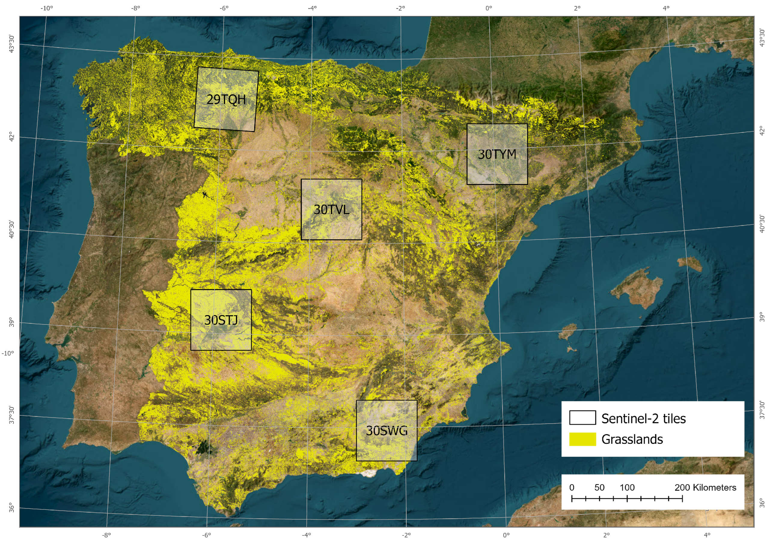
This study was carried out in mainland Spain, a region selected for its pronounced spatial heterogeneity and ecological richness. The territory hosts a wide variety of ecosystems and is particularly notable for its extensive and diverse grassland areas that amount to 32,097.96 km², ranging from arid lowland plains to humid high mountain areas [30] (Figure 1).

Five representative regions of interest, including the diversity of pasture dynamics, were selected based on land use information, climatic conditions, and remote sensing data using the Spanish Common Agricultural Policy Geographical Identification System (SIGPAC), the Köppen climate classification and the boundaries of Sentinel-2 tiles, respectively. By overlaying SIGPAC data with climatic strata, we identified the Sentinel-2 Military Grid Reference System (MGRS) tiles that cover the largest grassland areas within the different geoclimatic regions. These tiles, namely 29TQH, 30STJ, 30TVL, 30SWG, and 30TYM [8], have a total of 14,031 plots and a total pasture surface of 851.74 km². Figure 1 shows their location and the spatial distribution of the grasslands (yellow).

2.2. Data Sources

2.2.1. NDVI Sentinel-2 Time Series

Sentinel-2, operated by the European Space Agency (ESA), carries the Multispectral Imager (MSI), an instrument that captures reflectance across 13 spectral bands at three different spatial resolutions: 10, 20 and 60 m, providing images at 5-day interval since 2017 [8]. In this study, the NDVI time series were derived from Sentinel-2 imagery—including both Sentinel-2A and Sentinel-2B satellites—at Level-2A processing (atmosphere and radiometric corrections applied) [31]. The imagery spans the period from January 2018 to December 2023 and covers the regions of interest (Figure 1). Data were downloaded from Microsoft’s Planetary Computer [32], an extensive open-access platform that hosts a wealth of satellite observations. To ensure temporal consistency and capture vegetation dynamics at a fine temporal resolution, the imagery was acquired from the same tile and the same orbit which has a revisit time of 5 days, independently of the cloud cover. If the image was not available for the expected acquisition date, a “blank date” was incorporated to maintain the Sentinel-2 5-day revisit cycle. This resulted in 438 observations for each time series.

NDVI time series were computed at three spatial resolutions (10, 20 and 60 m) using the standard formula: NDVI = (${\rho }_{nir}$ – ${\rho }_{red}$)/(${\rho }_{nir}$ + ${\rho }_{red}$) [4]. Band 4 served as red reflectance across all resolutions, while we selected Band 8 for 10 m and Band 8A for 20 and 60 m as near-infrared reflectance (

Table 1. Sentinel-2 spectral bands for red (${\rho }_{red}$) and near-infrared (${\rho }_{nir}$) reflectance selected for each spatial resolution (10, 20 and 60 m).

	Resolutions (m)
	10	20	60
${\rho }_{red}$	B4	B4	B4
${\rho }_{nir}$	B8	B8A	B8A

). For the 60 m data, we relied on ESA’s standard Level-2A product, which applies Sen2Cor [31] atmospheric correction and spatial aggregation automatically. This approach guarantees reproducibility and sidesteps the artifacts that can arise when applying custom resampling algorithms.

A sensitivity check has been conducted to ensure that the radiometric bias caused by the use of two different near-infrared bands (B8 and B8A), which overlap but do not share the same characteristics, does not affect the results. For further information, see Supplementary Materials Table S2.

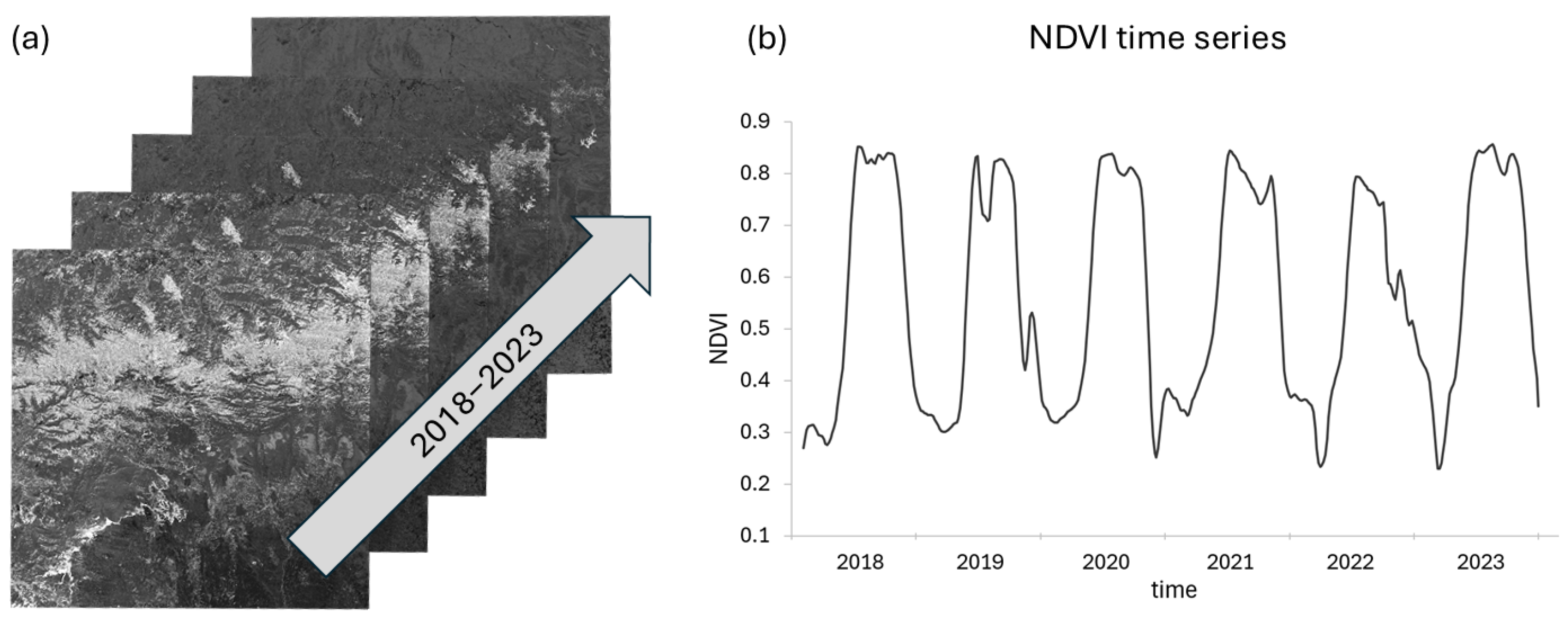
To generate pixel-based NDVI time series, Sentinel-2 images were stacked in chronological order. To ensure temporal consistency, the Sentinel-2 5-day revisit cycle was maintained by incorporating “blank dates” when images were not available for the expected acquisition date. In addition, the data quality assessment was based on the Scene Classification Map (SCL). Observations were labeled as invalid when classified as “no data,” “saturated or defective,” “dark area pixels,” “cloud shadows,” “cloud medium probability,” “cloud high probability,” “snow” or “thin cirrus”. The missing and invalid observations were imputed by linear interpolation procedure with no window. A harmonization step was conducted to correct reflectance inconsistencies across spectral bands following the anomaly that occurred on 24 January 2022 [8], ensuring comparability throughout the study period. The time series was then smoothed using a Savitzky–Golay filter, which is commonly used in remote sensing applications and is based on the least squares method [33]. In particular, we used a window size of 5 and a polynomial degree of 2 to ensure optimal noise reduction while preserving the integrity of the signal [34]. The final product is a data cube per region of interest that includes filtered NDVI time series on a pixel basis (Figure 2).

To quantify the amount of significant information contained in a pixel-based time series, the Interpolating Efficiency Indicator (IEI) was used [35]. The IEI was specifically designed considering both the frequency of invalid observations and the occurrence of extended gaps, considering their length and timing throughout the year. Although short gaps spanning only one to three consecutive invalid points are typically interpolated with high confidence, the reliability of interpolation decreases significantly when encountering longer gaps, especially if they coincide with key phases of the growth cycle [35]. The IEI ranges from 0 to 100; with higher values revealing a greater capacity of the original time series to preserve crucial information for applications such as phenological assessments, crop development monitoring, and broader time series analyses. The weighting factors used in the IEI reflect the assumption that larger interruptions exert a disproportionately negative impact on the overall series, requiring heavier weights to properly account for their influence. In this study, the IEI was used to remove plots with insufficient data quality for a reliable comparison. All plots with an IEI below 90 were excluded from further analysis.

2.2.2. Data Acquisition and Processing

The download and processing of the satellite imagery time series (2018–2023, 438 observations distributed across 5 tiles) were implemented using automated routines in a Python environment (version 3.12). Access to and querying of the SpatioTemporal Asset Catalog (STAC) catalogs were managed using the Microsoft planetary computer [32] and pystac [36] libraries, while the ingestion and multidimensional structuring of the spatial data were performed with xarray, rioxarray, and odc.stac libraries.

To optimize the computational demand during the calculation of spectral indices, the Just-In-Time (JIT) compilation of numba [37] was combined with the distributed processing capabilities of dask [38] libraries. All operations were executed on a server equipped with 40-core Intel Xeon Gold processors and 256 GB of RAM, employing a data chunking strategy of [1024, 1025, 10]. The final results were exported in Cloud Optimized GeoTIFF (COG) format with DEFLATE compression.

2.2.3. Köppen-Geiger Climate Classification

To capture the diversity of grassland dynamics, regions of interest were selected from the major climatic regions. For this purpose, the Köppen climate classification was selected, as it is one of the most widely used systems for categorizing the world’s climates based on temperature and precipitation patterns [39]. The grasslands of the study area are mainly located in dry (B) and temperate (C) climates [40]. Further subcategories are defined by additional letters according to seasonal and precipitation characteristics. Thus, the second letters describe precipitation patterns (e.g., f for no dry season, w for winter dry, s for summer dry) and the third letters indicate temperature characteristics (e.g., a for hot summers, b for warm summers, c for cool summers). In particular, the Mediterranean hot-summer climate (Csa) is the most widely extended throughout the study area, mainly in the southern central plateau and the Mediterranean coastal regions. Temperate climates without a dry season (Cfa and Cfb) are found mainly along the northern Atlantic coast, as well as in the Iberian Mountain ranges, the Pyrenees, and surrounding areas. Dry climates are in the southeast of Spain and in the Ebro Valley. The Köppen Climate Classification and Corresponding Codes for the Iberian Peninsula are shown in Table S1 and their spatial distribution is shown in Figure S1, located in Supplementary Materials Table S1. As grasslands are not distributed uniformly across the territory, it has been decided, for further analysis, to combine these climates into three groups: B, Cs and Cf.

2.2.4. Geographic Information System for Agricultural Parcels in Spain (SIGPAC)

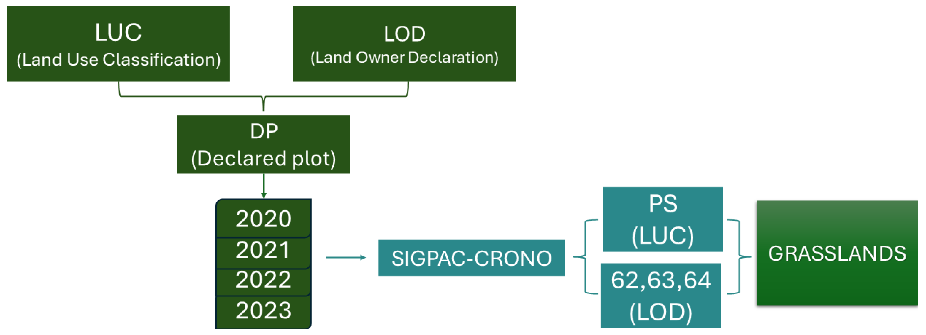
To spatially delimit grassland plots, the Spanish Land Parcel Identification System (LPIS), known as SIGPAC, was used [30]. It is a key technical and administrative support tool for implementing the Common Agricultural Policy (CAP), providing georeferenced parcel boundaries that facilitate government functions such as subsidy allocation, land planning, and regulatory compliance. This system also integrates remote sensing and field data for improved agricultural monitoring. In addition, SIGPAC delivers annual layers of land-use classification and land owners’ declarations; linking these two datasets temporally ensures consistency throughout the study period. For the purpose of this study, the Spanish Agricultural Guaranty Fund provided the annual SIGPAC records from 2020 to 2023. Based on this information, a new geospatial layer called SIGPAC Crono (Figure 3) was developed to integrate and temporally align the multi-year data. This new layer improves the temporal consistency of the original database and includes both land use classifications and declared agricultural practices reported by landowners over this 4-year period. To ensure the reliability and consistency of our land use data, we selected plots based on SIGPAC Crono continuously declared by landowners as permanent grasslands or classified as grasslands during 2020–2023. A total of 14,031 plots met this criterion, which represents 851.74 km².

Although the NDVI time series encompasses the 2018–2023 period, the reference land-cover data was derived from SIGPAC records strictly for the 2020–2023 timeframe. This temporal discrepancy is justified by the fact that the declared agricultural practices—essential for the accurate identification and classification of these specific grassland typologies—were only integrated into the SIGPAC database from 2020 onwards. Given that these grasslands constitute highly stable vegetative formations, and their persistence was confirmed through multi-year analysis (2020–2023) rather than a static annual layer, the assumption of land-cover stability was reliably extended to the 2018–2019 period without compromising the integrity of the analysis.

2.3. Methodology

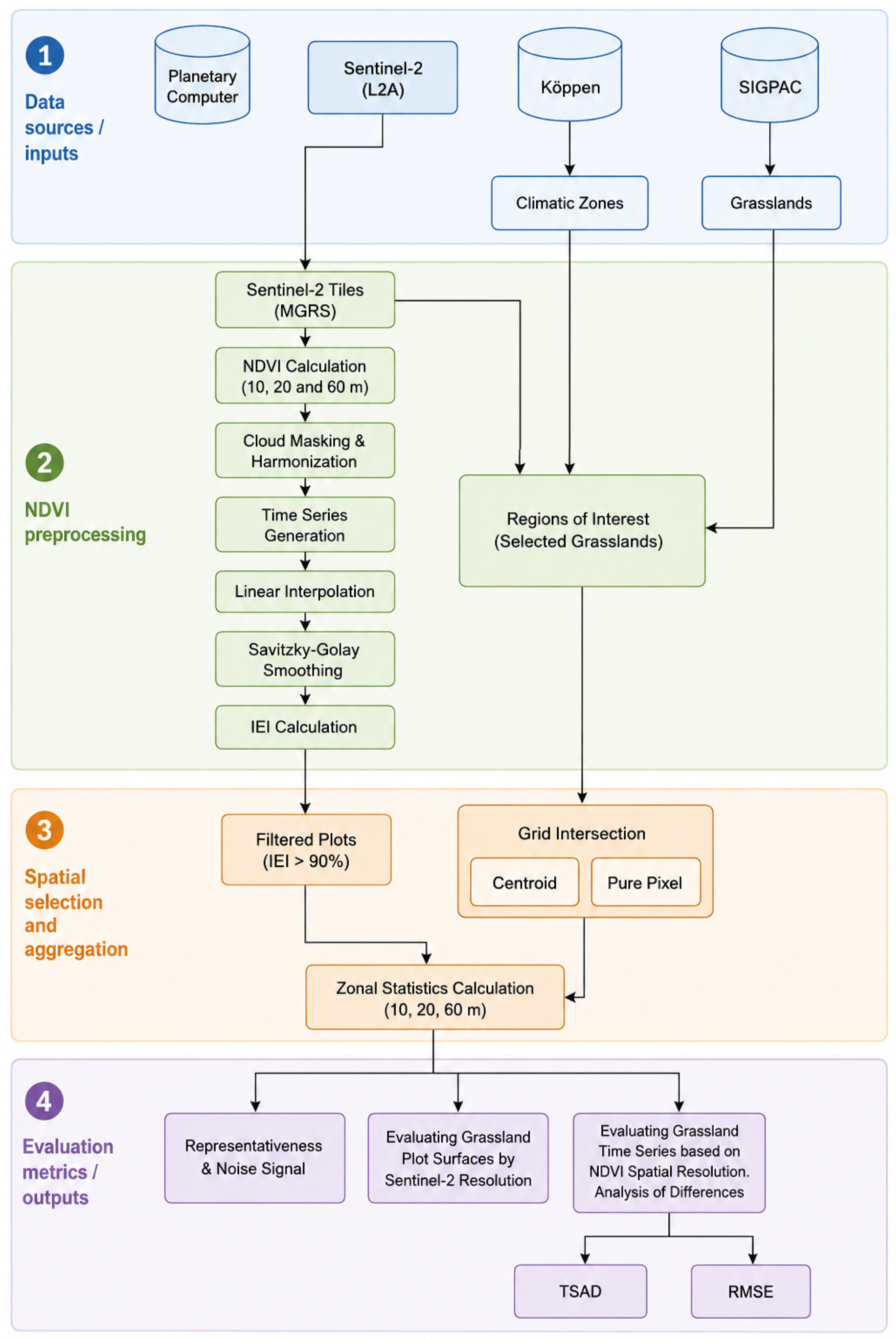
Figure 4 shows the workflow that details the integrated approach used to analyze grassland dynamics in Spain based on Sentinel-2 satellite imagery. By overlaying geoclimatic strata with SIGPAC data, we identified Sentinel-2 tiles that cover the largest grassland areas within the different geoclimatic regions. For the selected Sentinel-2 tiles, the NDVI time series were generated at multiple spatial resolutions (10, 20, and 60 m), applying rigorous data harmonization, cloud masking and interpolation procedures. The quality and consistency of the time series were systematically assessed using the Interpolation Efficiency Indicator (IEI) proposed by Sáenz et al. [35]. Spatial accuracy analyses were conducted using both centroid and pure-pixel methods, allowing for comparisons across different spatial resolutions. Additionally, grassland dynamics was evaluated using the Time Series Angle Distance (TSAD) technique [41] and the Root Mean Square Error (RMSE) metric [42]. This methodological framework allowed for a consistent and comprehensive evaluation of grassland evolution within representative ecological contexts. The methodology described is essential in environmental monitoring and land-cover change studies, as spatial resolution directly impacts the precision of vegetation analyses and the reliability of subsequent decision-making processes [28].

2.3.1. Assesment of the Spatial Resolution Impact on the Area and Number of Plots

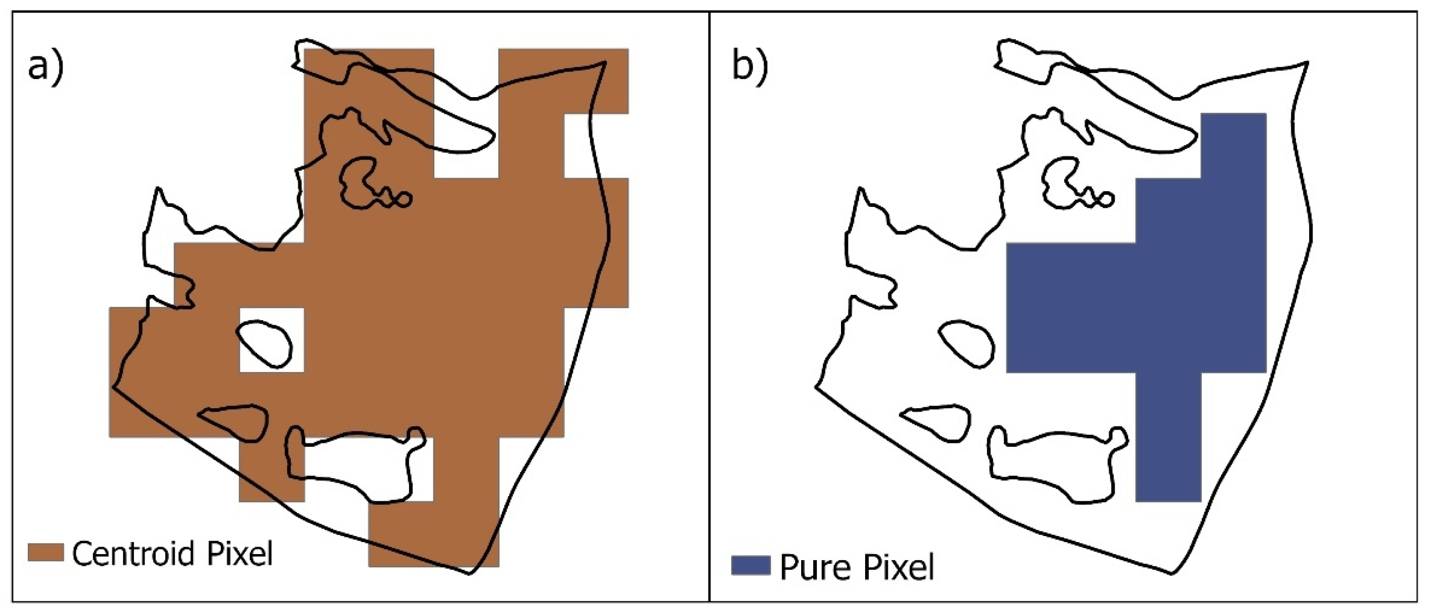
The effect of spatial resolution on grassland plots was assessed using two spatial aggregation approaches: the pure-pixel and centroid methods, which represent contrasting strategies for assigning Sentinel-2 pixels to agricultural parcels. In the pure-pixel method, only pixels fully contained within parcel boundaries are used. Rather than assuming ecological purity at the sub-pixel level, this approach ensures that the selected pixels respect the thematic homogeneity of the parcel as classified by the SIGPAC. This avoids spectral mixing with adjacent land covers and aligns with our main objective: analyzing the temporal dynamics of the parcel as a whole management unit, rather than the dynamics of individual pixels [21]. By contrast, the centroid method assigns any pixel whose centroid falls inside the parcel, capturing finer spatial details and preserving the parcel’s irregular edges, even if some pixels straddle boundaries [21]. Figure 5 shows the effect of both approaches in the selection of pixels from grasslands plots. The pure-pixel-based approach yields a coarser, less natural delineation of parcel shapes; however, it reduces systematic bias in land-cover estimates by mitigating edge effects during the assessment of grassland dynamics. In contrast, while the centroid approach provides a more detailed and natural parcel delineation, it introduces artificial spatial patterns that can distort the original geometry and compromise spatial precision.

Within the regions of interest, both the pure-pixel and centroid methods were used to estimate the following metrics at the three spatial resolutions (10, 20, and 60 m): (i) the number of plots evaluated, (ii) the minimum plot area, (iii) the average plot area, and (iv) the total plot area. Comparing these metrics enabled the assessment of information loss in terms of surface area and number of evaluated plots as the spatial resolution of the input data decreased.

2.3.2. Representativeness and Spatial Signal-to-Noise Ratio (SSNR)

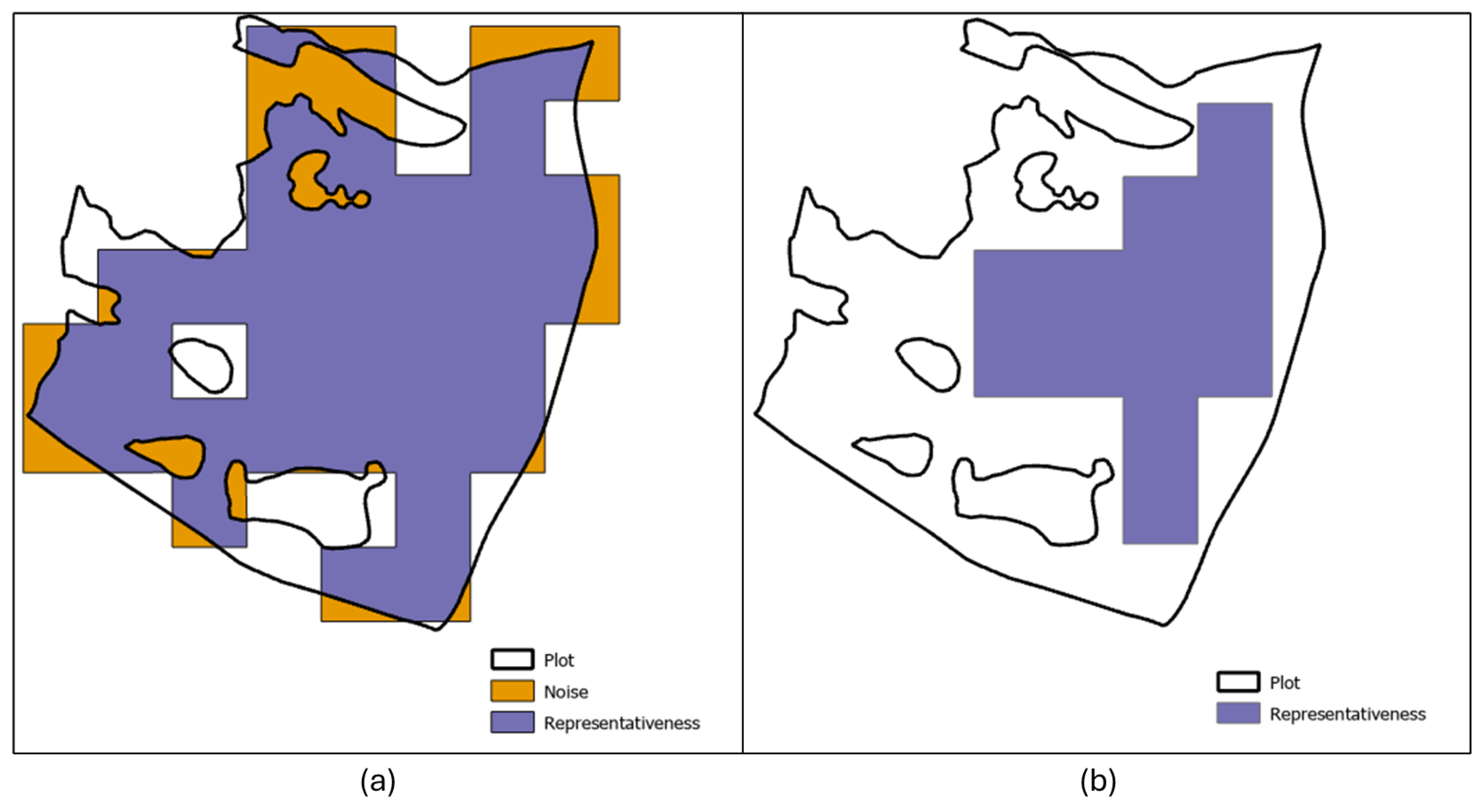
To assess the spatial accuracy of the NDVI data within the study plots, two metrics were considered: representativeness and Spatial Signal-to-Noise Ratio (SSNR). Representativeness refers to the proportion of the plot that is effectively covered by Sentinel-2 pixels [43]. The representativeness ranges from 0 to 1, with 1 indicating a perfect match between the plot boundary and Sentinel-2 pixels. In contrast, noise corresponds to the portion of Sentinel-2 pixels assigned to a plot for the NDVI calculation that lies outside the physical boundaries of the plot. The SSNR is calculated as the ratio of representativeness to noise according to Equation (1) [43]. SSNR values range from 0 to infinity, with higher values indicating better spatial representativeness. The SSNR metric is only applicable to the centroid method. By definition, the pure-pixel strategy strictly selects pixels fully contained within the parcel boundaries, resulting in zero spatial noise and rendering the SSNR mathematically infinite.

$$SSNR=10\times {\log }_{10}(\mathrm{representativeness}/\mathrm{noise})$$

(1)

Figure 6 illustrates the areas of representativeness (the portion of a pixel inside the plot) and noise (the portion of a pixel outside the plot), which are derived from two methods: (a) the centroid method and (b) the pure-pixel method. When using the pure-pixel method, there is no noise signal, which increases the reliability of vegetation indices compared to the centroid method, especially in heterogeneous landscapes where edge effects and partial inclusion of pixels can significantly bias the results [44]. When using the centroid method, it is important to obtain the highest possible SSNR metric, which depends on the spatial resolution. Accurate characterization of these metrics supports a more robust interpretation of time series data and improves the reliability and fidelity of remote sensing analyses in ecological applications [45].

2.3.3. Assessment of the Spatial Resolution Impact on the NDVI Time Series

The mean NDVI time series was extracted for each plot to analyze the temporal NDVI variations between the selected parcels. The mean NDVI values for the selected pixels were calculated based on both the centroid and pure-pixel criteria, considering all spatial resolutions of 10, 20 and 60 m. Differences among mean NDVI time series were evaluated using two metrics: Time Series Angle Distance (TSAD) and Root Mean Squared Error (RMSE). Pairwise comparisons enabled the assessment of how spatial resolution degradation affects NDVI interpretation and helped identify the impacts of pixel mixing on vegetation spectral variability. The pure 10 m resolution was selected as the baseline for comparison, as it provides the most accurate representation of the grassland plots.

Table 2. Study cases performed for the comparison between spatial resolutions.

		Centroid			Pure
		10	20	60	10	20	60
Pure	10	X	X	X		X	X

offers a visual overview of the different combinations of resolution analyzed, allowing a direct comparison against this baseline case.

Time Series Angle Distance (TSAD).

The Spectral Angle Mapper [41] method was originally developed to quantify spectral similarity by measuring the angle between spectral vectors in an n-dimensional space. In this study, the method is adapted and renamed Time Series Angle Distance (TSAD) to compare temporal patterns—specifically, time series of mean NDVI values at the plot level. TSAD measures the angle between per-plot average values at different resolutions, thus providing a metric that quantifies the similarity of temporal signatures in n-dimensional space. TSAD is calculated according to the following equation and varies between 0 and $\pi$, the lower values mean the convergence between the time series Equation (2).

$$\mathrm{TSAD}(s_1,s_2)={\cos }^{-1}\left({\displaystyle \frac{{\sum }_{i=1}^N\left(s_{1,i}{s}_{2,i}\right)}{\sqrt{{\sum }_{i=1}^N{s}_{1,i}^2}·\sqrt{{\sum }_{i=1}^N{s}_{2,i}^2}}}\right)$$

(2)

where $s_1$ and $s_2$ represent the mean NDVI time series for the first and second spatial resolutions being compared, $s_{1,i}$ and $s_{2,i}$ denote the NDVI values at the specific time step i, and N is the total number of temporal observations in the series.

Root Mean Squared Error (RMSE).

The RMSE metric, derived from the standard deviation of residuals, was used to evaluate the consistency of the NDVI time series across Sentinel-2 resolutions and spatial aggregation methods by quantifying the average deviation from the baseline NDVI values. Baseline data were obtained at 10 m using the pure-pixel method, while comparisons included centroid-based data at 10, 20 and 60 m and pure-pixel data at 20 and 60 m. The NDVI values for each series were aligned so that the observations at time t corresponded to the same date in both resolutions. The errors were then calculated as the differences between the baseline values ($Y_t$) and the compared resolution values ($X_t$). These differences were squared, averaged over the total number of time observations (N), and finally square-rooted to obtain the RMSE, expressed as

$$RMSE=\sqrt{{\displaystyle \frac{{\sum }_{t=1}^N{(X_t-Y_t)}^2}{N}}}$$

(3)

The closer this value is to zero, the greater the similarity between the NDVI time series, while higher values indicate more pronounced discrepancies [42]. Thus, TSAD and RMSE metrics therefore help determine the extent to which different Sentinel-2 spatial resolutions produce coherent NDVI values, aiding in evaluating their reliability for specific applications.

2.3.4. Influence of Plot Size and Climate on Spatial Resolution Effects

Given the large sample sizes involved in this study ($n>4000$ in most strata), statistical significance from the Kruskal–Wallis test does not, by itself, indicate the practical magnitude of the observed differences [46]. To complement the significance tests, we estimated effect sizes for both the overall comparison among climate-based strata and for plot size classes, for each of the resolution–aggregation methods.

Omnibus Kruskal–Wallis test.

For each of the five resolution–agregation methods and each error metric (RMSE and TSAD), we tested whether the metric differed across the categories of two environmental grouping variables—parcel-size category and Köppen climate group—using the Kruskal–Wallis H test [47]. Effect size was quantified using epsilon-squared (${\epsilon }^2$) (4), a non-parametric analogue of eta-squared (${\eta }^2$) in ANOVA:

$${\epsilon }^2={\displaystyle \frac{H}{n-1}}$$

(4)

where H is the Kruskal–Wallis test statistic and n is the total sample size across all categories being compared [48]. ${\epsilon }^2$ ranges from 0 to 1 and represents the proportion of variance in the ranked data explained by group membership. Values were interpreted following the conventional thresholds proposed by Cohen [49], commonly applied to ${\epsilon }^2$ and ${\eta }^2$: negligible (${\epsilon }^2<0.01$), small ($0.01\le {\epsilon }^2<0.06$), medium ($0.06\le {\epsilon }^2<0.14$), and large (${\epsilon }^2\ge 0.14$).

Pairwise comparisons among methods.

Within each stratum category, all pairwise combinations of these methods were compared using the paired difference D between methods for each sampling unit. Pairwise deletion was used, retaining all units with valid data for the specific pair being compared, regardless of missing values in unrelated methods. The matched-pairs rank-biserial correlation (Cliff’s Delta) was computed for these comparisons, based on the sign of the within-pair difference Equation (5).

$${\delta }_{\mathrm{paired}}={\displaystyle \frac{n(D>0)-n(D<0)}{n}}$$

(5)

The effect size ${\delta }_{\mathrm{paired}}$ ranges from −1 to 1. A positive sign indicates that the first method systematically yields higher values than the second, while a negative sign indicates the opposite. A value of 0 implies complete stochastic equality between the methods. The magnitude classes were defined following Romano et al. [50] and applied to the absolute value $|{\delta }_{\mathrm{paired}}|$ (negligible < 0.147, small 0.147–0.33, medium 0.33–0.474, large ≥ 0.474). Pairwise comparisons were summarized visually as method × method effect-size matrices, faceted by metric and stratum category matrices, faceted by metric and stratum category.

3. Results

3.1. Impact of the Spatial Resolution on the Area and Number of Plots

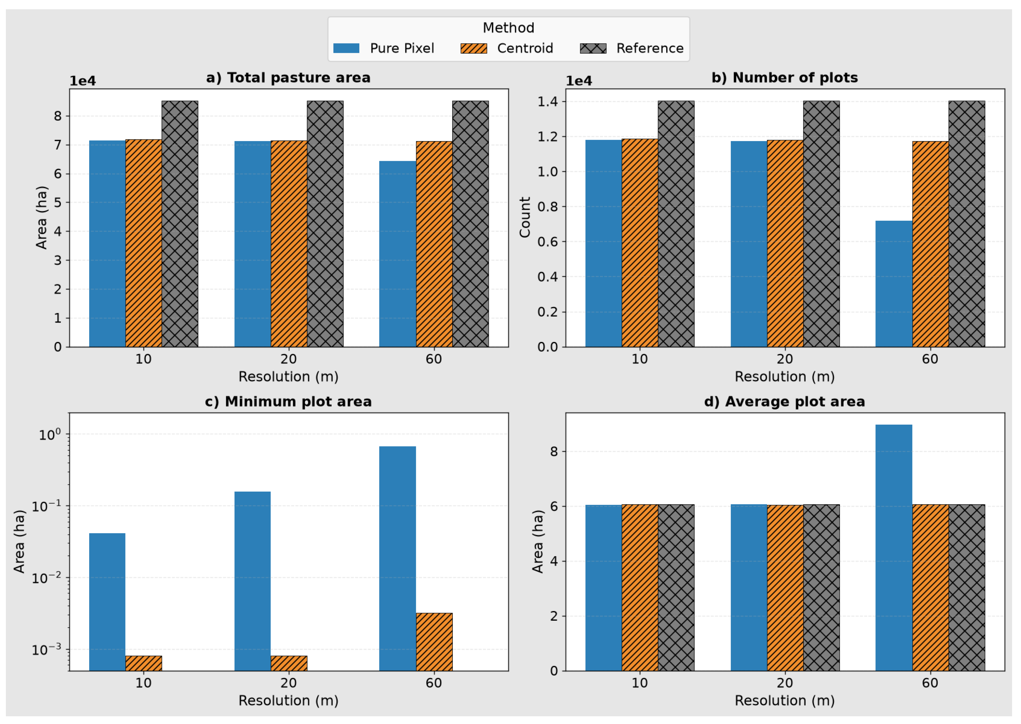
Figure 7 illustrates the descriptive statistics for the plots obtained using SIGPAC crono and shows how the results of the analysis vary depending on the resolution and spatial aggregation method used. The differences in total grassland area (Figure 7a) were almost imperceptible among the spatial aggregation methods at the 10 m and 20 m resolutions. In contrast, at the 60 m resolution, there was a noticeable reduction in the total area when using the pure-pixel method. Regarding the number of plots (Figure 7b), there were no significant differences at 10 and 20 m resolutions, while more than half of the plots were lost when using the pure-pixel method at 60 m resolution across all tiles. Furthermore, a comparison of Figure 7a,b revealed that approximately half of the plots were relatively small (less than 500 m²), representing only about 10% of the total area. In contrast, the centroid-based method with a resolution of 60 m retained all parcels and preserved the grassland area in the study region, while still maintaining the edge effect. The results clearly showed that as spatial resolution decreases, the minimum plot area increases—an effect particularly noticeable with the 60 m pixel size—as illustrated in Figure 7c. For the analysis of the average plot area (Figure 7d), a consistent pattern was observed at the 10 and 20 m resolutions, where values remained stable or increased slightly. In contrast, at the 60 m resolution, the average area increased substantially using pure-pixel approach. These findings indicate that coarser spatial resolutions tend to inflate average area measurements, due to the loss of small plots.

3.2. Representativeness and Spatial Signal-to-Noise Ratio (SSNR) of the Study Plots

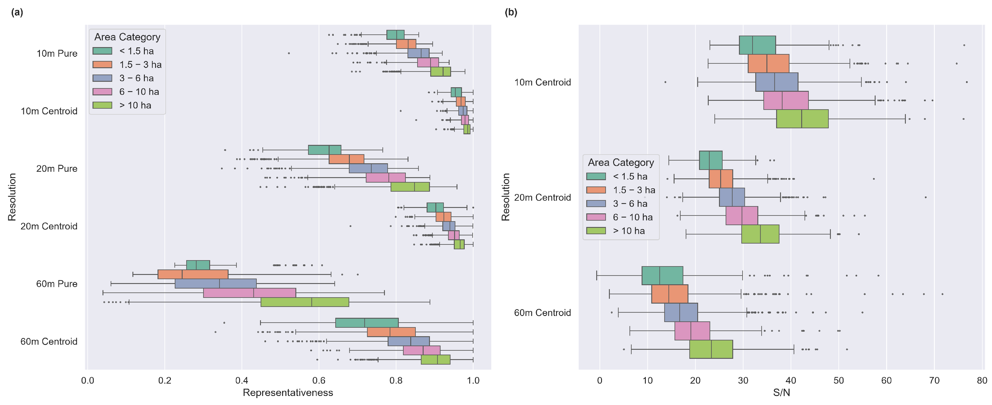
Figure 8 shows boxplots of the representativeness metrics (a) and SSNR (b) in five categories of parcel area, grouped by spatial resolution and aggregation method. General patterns of these metrics were observed according to the spatial resolution, spatial aggregation method, and parcel size. For the representativeness metric, the pure-pixel method yielded lower values and generally higher variability (i.e., wider boxplots) than the centroid method across all spatial resolutions. When comparing spatial resolutions, the 10 m resolution generally showed the highest representativeness values with lower variability, whereas the 60 m resolution showed the lowest with higher variability. In addition, this metric increases with the area of the parcel, so that most of the higher values were found in parcels with higher area (>10 ha). In particular, the smallest parcels (<1.5 ha) showed low variability when the pure-pixel method was applied at 60 m resolution, in contrast to parcels of equivalent area at the same resolution when the centroid method was used. The Spatial Signal-to-Noise Ratio (SSNR) improved with the increase in spatial resolution, so higher values were found at 10 m spatial resolution. In addition, this metric increases with the size of the parcel in all spatial resolutions, finding the highest values in parcels with a larger area (>10 ha). In general, the highest spatial variability across all parcel area categories is found at a 10 m spatial resolution.

3.3. Impact of Spatial Resolution on NDVI Time Series

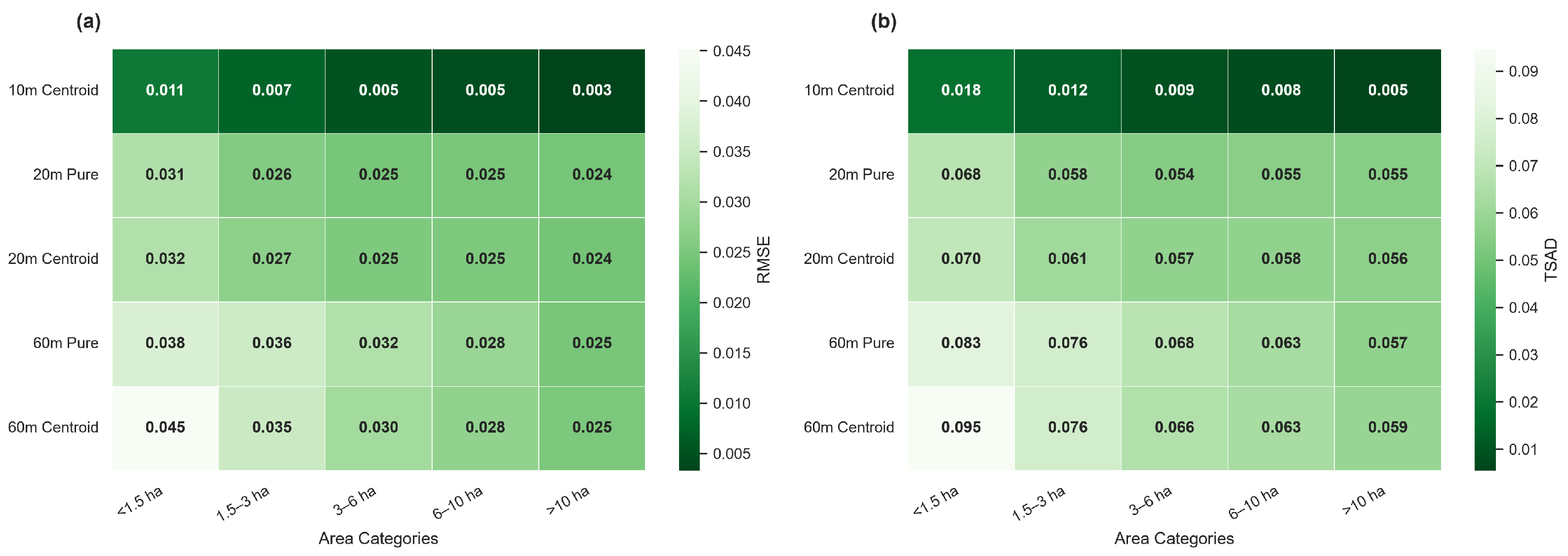
Figure 9 shows the mean values of TSAD (a) and RMSE (b) in the different parcel size categories. For both metrics, the parcel time series at 10 m spatial resolution using the pure-pixel approach was used as a baseline for the comparisons. The results indicate that variations in the temporal dynamics of the NDVI are primarily driven by spatial resolution and secondly by the area and aggregation strategy of the parcel. The mean TSAD and RMSE values increase with decreasing spatial resolution. At a constant 10 m resolution, comparing the centroid method to the pure-pixel baseline yields very low errors (<0.02) across all area categories, indicating high temporal consistency. In contrast, both 20 m and 60 m resolutions showed substantially higher mean TSAD and RMSE values than at 10 m: in some cases, even ten times greater than those at 10 m. However, the increase in magnitude is greater when comparing time series between 10 m and 20 m than between 20 m and 60 m. In addition, the centroid method tends to produce slightly higher TSAD and RMSE values than the pure-pixel approach in most parcel sizes, this effect being more pronounced for the smallest parcels (<1.5 ha). The parcel size also modulates these metrics, although to a lesser extent than spatial resolution. The smallest parcels (<1.5 ha) consistently exhibit the highest TSAD and RMSE values in every combination of resolution-method. Overall, the lowest mean values of both metrics are obtained with 10 m centroid data in parcels larger than 10 ha, while the highest mean values occur at 60 m centroid for parcels smaller than 1.5 ha.

The results of the omnibus Kruskal–Wallis test, summarized in

Table 3. Results of the omnibus Kruskal–Wallis test evaluating the effect of parcel area and Köppen climate classification on TSAD and RMSE metrics across different Sentinel-2 spatial resolutions and aggregation methods. Effect sizes are quantified using epsilon-squared (${\epsilon }^2$) with their corresponding magnitude: negligible (no color), small (green), medium (blue), large (red). Statistical significance is indicated as follows: *** p < 0.001.

AREA
TSAD							RMSE
Method	H Stat.	p-Value	n	${\mathit{\epsilon }}^{\mathbf{2}}$	Magnitude		Method	H Stat.	p-Value	n	${\mathit{\epsilon }}^{\mathbf{2}}$	Magnitude
10 m Centroid	2036.5	***	7461	0.273	Large		10 m Centroid	1743.0	***	7461	0.234	Large
20 m Pure	158.4	***	7411	0.021	Small		20 m Pure	260.8	***	7411	0.035	Small
20 m Centroid	320.0	***	7453	0.043	Small		20 m Centroid	443.2	***	7453	0.060	Small
60 m Pure	575.5	***	4653	0.124	Medium		60 m Pure	848.8	***	4653	0.183	Large
60 m Centroid	1133.8	***	7404	0.153	Large		60 m Centroid	1357.2	***	7404	0.183	Large
KOPPEN
TSAD							RMSE
Method	H Stat.	p-Value	n	${\mathit{\epsilon }}^{\mathbf{2}}$	Magnitude		Method	H Stat.	p-Value	n	${\mathit{\epsilon }}^{\mathbf{2}}$	Magnitude
10 m Centroid	400.9	***	7461	0.054	Small		10 m Centroid	298.1	***	7461	0.040	Small
20 m Pure	3310.6	***	7411	0.447	Large		20 m Pure	350.7	***	7411	0.047	Small
20 m Centroid	2893.7	***	7453	0.388	Large		20 m Centroid	681.4	***	7453	0.091	Medium
60 m Pure	1306.8	***	4653	0.281	Large		60 m Pure	213.7	***	4653	0.046	Small
60 m Centroid	1775.3	***	7404	0.240	Large		60 m Centroid	694.5	***	7404	0.094	Medium

, revealed that all methodological combinations yielded highly significant results ($p<0.001$), due to the large sample size analyzed at the individual plot level. Consequently, the interpretation of the discrepancies in the NDVI time series had to focus strictly on the effect size (${\epsilon }^2$, Table 3), which allowed for the discrimination of the true magnitude of the empirical influence exerted by the plot area and climatic conditions on the extracted spectral dynamics. The analysis of the impact of the plot area demonstrated that this variable strongly conditioned the error metrics when the centroid method was used at a maximum resolution of 10 m. In this scenario, both TSAD and RMSE showed a large effect size (${\epsilon }^2$ of 0.273 and 0.234, respectively; Table 3), which reflected the strong penalty from the edge effect and the subsequent spectral contamination from adjacent land covers in the plots. However, when scaling to the 20 m resolution, the influence of the area was drastically diluted to a small magnitude in both the pure-pixel and centroid strategies. This suggested that the 20 m pixel homogenized the intrinsic variability linked to the dimensions of the plot. When degrading the resolution to 60 m, the effect size became large again (Table 3), evidencing that this coarse spatial resolution severely compromised representativeness and introduced critical spectral mixing in the plots. Furthermore, the results showed that the Köppen climate classification exerted a markedly asymmetrical influence on TSAD and RMSE (Table 3). Climate decisively determined the shape of the time series (TSAD) when the resolution was reduced to 20 m and 60 m, where consistently large effect sizes were recorded (reaching ${\epsilon }^2$ values of up to 0.447). This indicated that spatial degradation distorted the NDVI phenological trajectory highly unequally depending on the bioclimatic environment of the plot. In sharp contrast, the influence of climate on the RMSE metric remained contained within small and medium magnitudes across all resolutions and methods (Table 3). This divergence highlighted that, although the use of 20 m or 60 m spatial resolutions severely deformed the temporal phenological signature depending on the climatic context, the absolute quantitative deviation of the average NDVI value within the plot did not experience such extreme variations across the different regions.

To better understand the differences between the resolution–aggregation strategies, we performed pairwise comparisons using Cliff’s Delta. This non-parametric effect size provides a deeper understanding of how the choice of spatial resolution and aggregation method consistently shifts the distribution of RMSE and TSAD values across different plot size and climate strata.

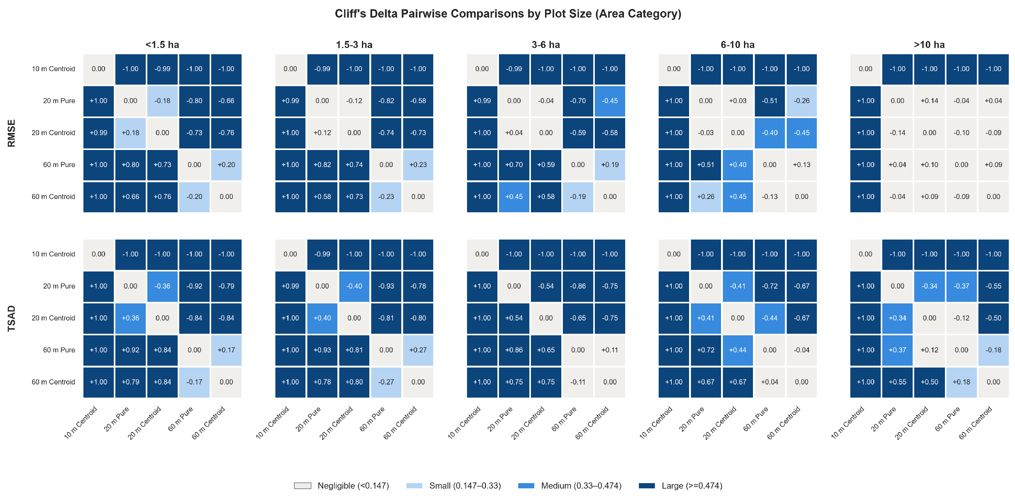
Pairwise Cliff’s Delta analysis stratified by plot size revealed a consistent pattern across both RMSE and TSAD metrics (Figure 10). The largest effect sizes were systematically associated with comparisons involving the 10 m spatial resolution, with Cliff’s Delta values frequently approaching $\left|\delta \right|=1$, indicating an almost complete separation between the distributions obtained at 10 m and those derived from coarser resolutions. Comparisons between the 20 m and 60 m datasets yielded substantially smaller effect sizes, suggesting that most methodological differences arise when moving from the native Sentinel-2 resolution to coarser resolutions. Likewise, comparisons between aggregation methods within the same spatial resolution generally yielded negligible to moderate effect sizes, particularly for RMSE, suggesting that the choice of aggregation method exerted a comparatively minor influence on the evaluated metrics.

The magnitude of the resolution effect also varied with plot size. For small parcels (<3 ha), pairwise comparisons between spatial resolutions consistently produced large effect sizes, whereas these differences progressively decreased with increasing plot area. In the largest parcels (>10 ha), most comparisons between the 20 m and 60 m spatial resolutions showed negligible or small effect sizes, indicating that the influence of spatial resolution diminishes as parcel size increases. This trend was more pronounced for RMSE, whereas TSAD showed moderate effect sizes between aggregation methods in some plot-size classes, suggesting a greater sensitivity of this metric to methodological differences.

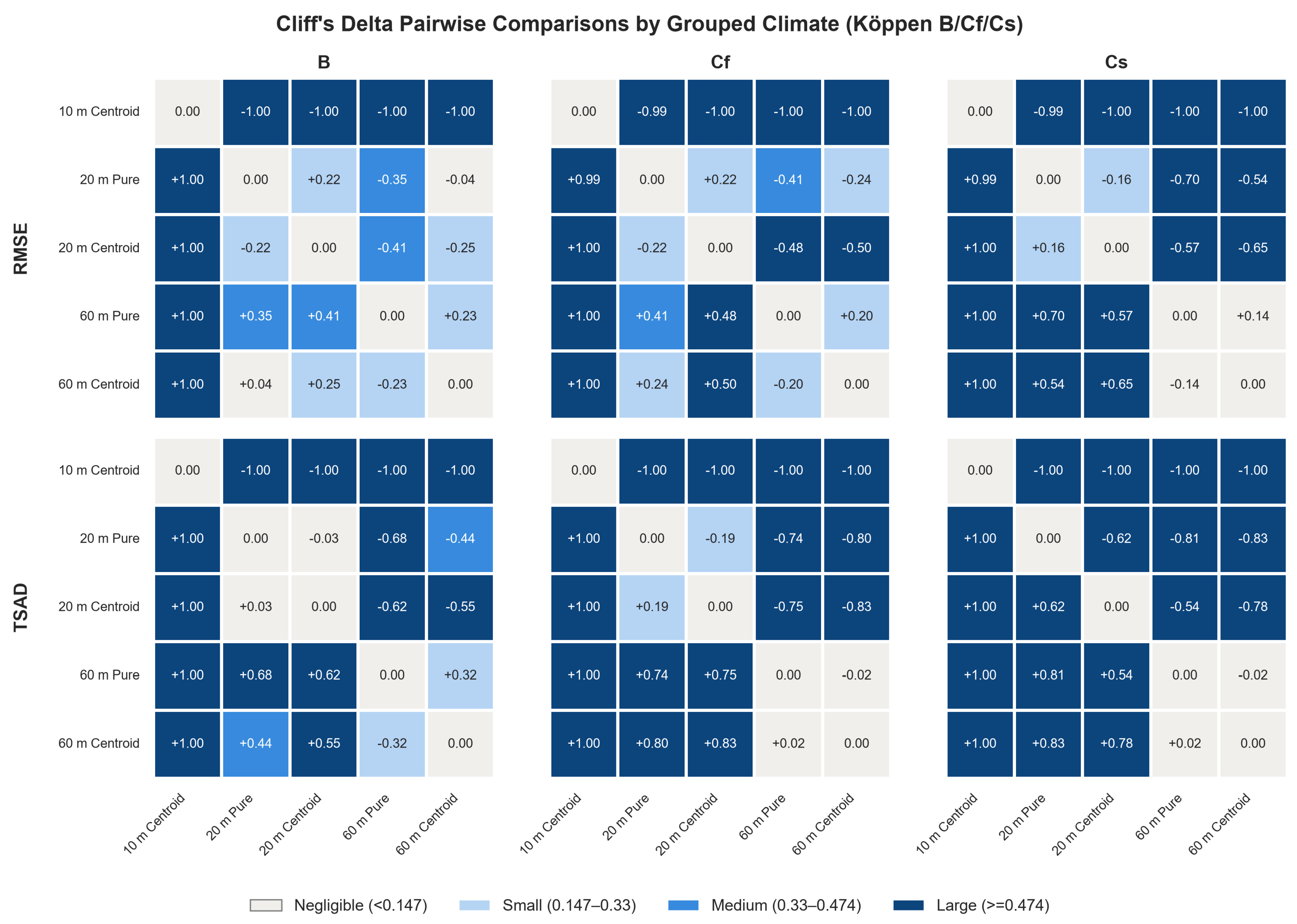
Pairwise comparisons based on Cliff’s Delta revealed a consistent effect on spatial resolution across the three grouped Köppen climates (B, Cf, and Cs) (Figure 11). In all climatic regions, comparisons involving the 10 m centroid strategy yielded effect sizes close to the maximum possible value ($\left|\delta \right|\approx 1$), indicating a systematic separation from all coarser-resolutions. This pattern was observed for both RMSE and TSAD, highlighting the strong influence of spatial aggregation relative to the 10 m baseline.

For the RMSE metric, effect sizes between the 20 m and 60 m resolutions were generally small to moderate and varied among climatic regions. In the B climate, comparisons between the pure and centroid strategies at the same spatial resolution produced negligible or small effects (e.g., $\delta$ = 0.22 for 20 m and $\delta$ = 0.23 for 60 m), whereas comparisons across different spatial resolutions reached moderate effect sizes. Similar patterns were observed in the Cf climate, although the differences between the 20 m and 60 m products tended to be slightly larger. In contrast, the Cs climate exhibited the strongest contrasts, particularly between the 20 m and 60 m products, with Cliff’s Delta values reaching up to $\left|\delta \right|=0.70$.

The TSAD metric exhibited a similar overall structure but generally larger effect sizes than RMSE. The differences between the 20 m and 60 m products were consistently moderate to large across all climatic regions, particularly in the Cf and Cs climates, where several pairwise comparisons exceeded $\left|\delta \right|=0.70$. Conversely, differences between the pure and centroid strategies at the same spatial resolution remained negligible to small, indicating that the aggregation strategy had a limited influence compared with changes in spatial resolution.

Together, these matrices provide a useful framework for identifying resolution–aggregation strategy combinations that yield comparable results across different climatic conditions and plot-size classes. Overall, these results indicate that spatial resolution is the primary driver of differences in both RMSE and TSAD, whereas the aggregation method plays a secondary role. The influence of spatial resolution was further modulated by both plot size and climatic conditions. Small grassland parcels were considerably more sensitive to changes in spatial resolution than larger parcels, while the largest effect sizes were generally observed under temperate climates (Cf and Cs). Furthermore, a notable difference between the two metrics emerged when comparing the pure and centroid aggregation strategies at the same spatial resolution. Whereas RMSE generally showed negligible or small effect sizes, TSAD frequently showed moderate effect sizes, indicating a greater sensitivity to changes in the aggregation strategy.

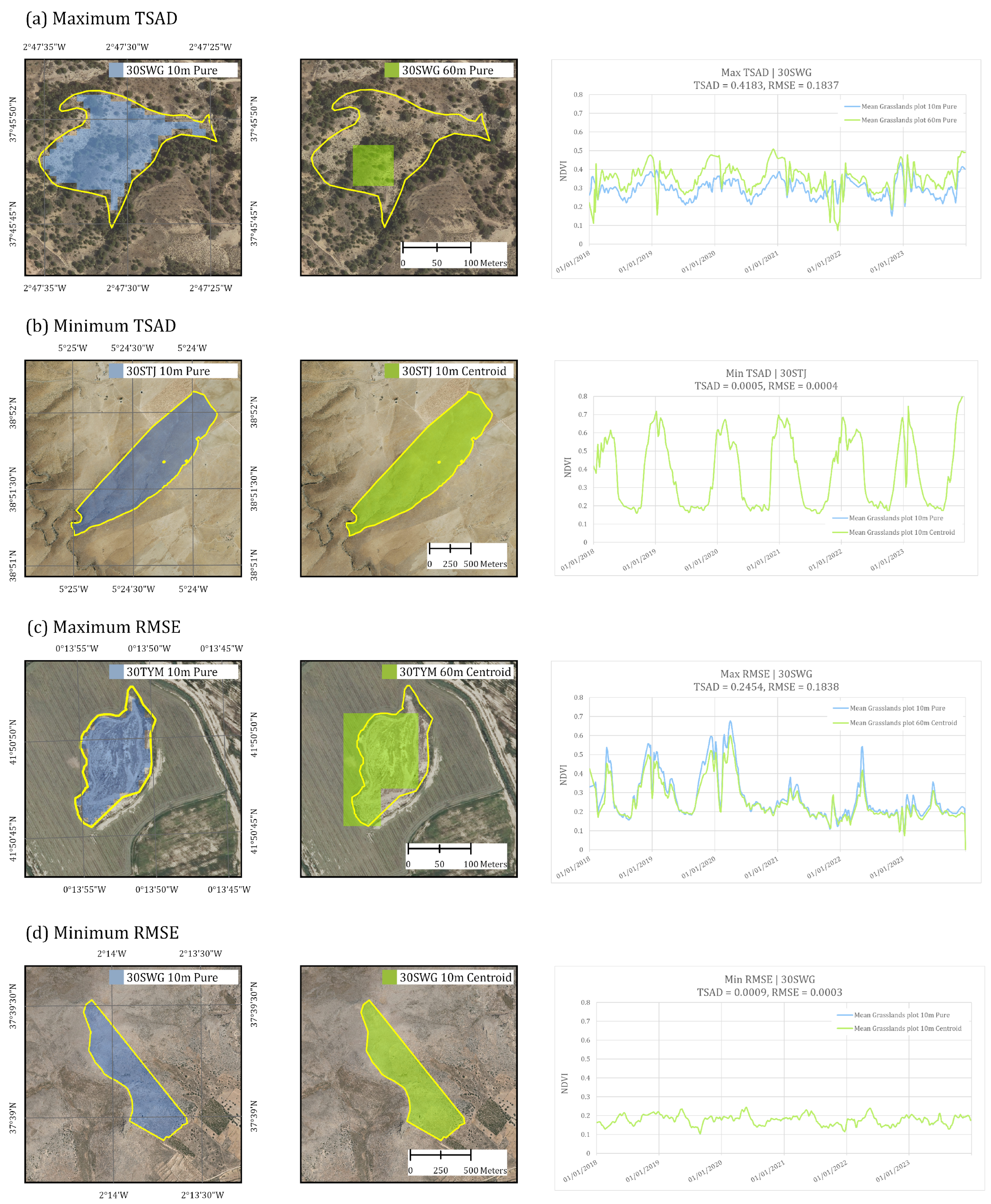
Figure 12 presents four representative grassland plots selected based on the maximum and minimum TSAD and RMSE values, as well as differences in their mean NDVI time series (2018–2023), all referenced to the baseline of 10 m pure-pixel method. Pixel selection and NDVI time series derived using pure-pixel and centroid approaches are shown in blue and green, respectively. The plots are displayed in yellow on a satellite imagery basemap. The figure illustrates how the choice of pixel-selection strategy and spatial resolution affects both the geometric representation of the plots—through the number, area, and spatial distribution of the selected pixels—and the spectral fidelity, reflected in the variations of the mean NDVI values. When TSAD and RMSE are minimum, there is a high similarity between mean NDVI time series. The differences between the mean NDVI time series increase as the TSAD and RMSE values increase. When comparing the most extreme values of both indicators, the largest discrepancies were associated with the highest TSAD values rather than with the highest RMSE values.

4. Discussion

We evaluated how methodological choices in image processing such as the spatial resolution (10 m, 20 m, 60 m) and pixel aggregation method (pure-pixel vs. cetroid) affect the selection of study plots, the spectral representation of the grassland plots and their NDVI time series consistency. The results revealed that the finer spatial resolutions of Sentinel-2 (i.e., 10 m, 20 m) are especially indicated for small plots (<3 ha) as they minimize the loss of the number of plots, preserving most of the total grassland area without significant differences between aggregation methods Figure 7. This is strongly supported by the omnibus Kruskal–Wallis test (Table 3), which demonstrated that plot area strongly conditions the error metrics at higher resolutions, particularly when using the 10 m centroid method, yielding a large effect size, with ${\epsilon }^2=0.273$ for TSAD and ${\epsilon }^2=0.234$ for RMSE. Furthermore, the pairwise comparisons using Cliff’s Delta (Figure 10) empirically validate that the discrepancies between the 10 m baseline and coarser resolutions become progressively more severe—transitioning to large effect sizes—in the smallest parcel categories (<1.5 ha and 1.5–3 ha). These small plots, which are located mainly in humid northern zones [51], show irregular boundaries where high resolution is required to accurately capture heterogeneity and estimate vegetation indices such as NDVI without excessive spectral mixing. As parcel area increases (>10 ha), the effect sizes decrease (Figure 10), suggesting that larger grasslands inherently mitigate the geometric distortions introduced by pixel-selection strategies.

Working at 20 m spatial resolution introduces a moderate but consistent phenological distortion (median TSAD = 0.05 rad, RMSE = 0.026), the majority of which is attributable to genuine resolution loss rather than pixel-extraction artifacts (pure-resolution TSAD = $0.049$ rad). Unlike the 60 m product, whose accuracy is strongly parcel-size dependent (Cliff’s $\delta$ = 0.68 vs. 0.35 at 20 m), the 20 m degradation remains within the “perceptible but non-severe” range across the full range of parcel sizes evaluated, supporting its use as a practical compromise between spatial detail and phenological fidelity for grassland monitoring at the parcel scale.

The choice between 10 and 20 m spatial resolution can be carried out using different criteria: (1) representativeness of NDVI dynamics with respect to grassland plots, and (2) time of processing of Sentinel-2 NDVI time series on a pixel basis. If the user prefers to obtain high spatial and temporal representativeness of NDVI dynamics, the 10 m should be chosen. This resolution showed higher values than 20 m in terms of spatial representativeness metric, especially when using the centroid method (Figure 8a). Furthermore, when using this aggregation method, the highest Signal-to-Noise Ratio was obtained at 10 m resolution (Figure 8b). In relation to the temporal representativeness of the dynamics of NDVI, the lowest TSAD and RMSE values were obtained at 10 m resolution compared to the 10 m pure-pixel baseline (Figure 9).

However, when the user aims to reduce both processing time and storage requirements for Sentinel-2 time series, the 20 m spatial resolution can be recommended. Using this resolution, only 50 plots were lost, equivalent to 124.48 ha. A critical factor in processing long-term satellite archives is the management of data volume, as minimizing memory footprint directly influences system throughput. The storage disparity between resolutions is substantial: a full Sentinel-2 time series (2018–2023) requires approximately 118 GB at 10 m resolution, whereas resampling to 20 m reduces this to 26 GB, representing a fourfold reduction. This decrease in data volume had immediate operational benefits. By reducing the memory load, our parallel processing pipeline was able to generate NDVI time series significantly faster.

Processing the full 5-tile dataset (2018–2023, 438 observations) required 5.2 h at 10 m resolution (118 GB output) and 1.5 h at 20 m resolution (26 GB output), representing a 72% speedup and 78% storage reduction

Table 4. Computational performance measured on Intel Xeon Gold 6248 × 2 (40 cores, 2.5 GHz), 256 GB RAM, dask chunking [1024, 1025, 10], GeoTIFF-COG output (DEFLATE level 9, 512 × 512 tiling).

Resolution	Processing Time	Storage	Memory Peak	Array Size
10 m	5.2 h	118 GB	128 GB	10,9802 × 438
20 m	1.5 h	26 GB	64 GB	54902 × 438
60 m	0.4 h	2.8 GB	16 GB	18302 × 438

. This improvement reflects the 16× reduction in array elements (4× fewer pixels per dimension), faster I/O throughput, and reduced memory pressure during parallel operations. These timings are hardware-dependent and not directly comparable to other systems; the relative speedup (2–3×) is expected to generalize across similar architectures.

Although TSAD and RMSE values at 20 m were three times higher than at 10 m (Figure 9), the vegetation signal remained largely preserved. Notably, even though the relative metric difference between 20 m and 60 m is smaller than the initial jump, the 60 m resolution suffered from significantly higher information loss due to the shape of the plots. Furthermore, these metrics presented small differences among pixel aggregation methods (pure and centroid based methods) (Figure 9). Thus, 20 m spatial resolution provides sufficient detail for most agricultural and biophysical applications while reducing data volume and processing time. This result is supported by recent studies showing that resolutions (20–30 m) can sufficiently capture vegetation dynamics in relatively homogeneous areas [13,15].

The use of a 20 m spatial resolution proved to be highly advantageous across the study area due to its robustness. Crucially, statistical analyses revealed that the effect of plot size on the temporal consistency of 20 m data is small for both TSAD and RMSE (${ϵ}^2<0.06$; Figure 10). This implies that 20 m imagery can be reliably applied for vegetation monitoring without a strict dependence on parcel dimensions, offering a versatile operational advantage. Despite this general stability, absolute metric values were lowest in plots larger than 10 ha (Figure 10), which are located mainly in the southern and central drylands [51]. Beyond parcel dimensions, our statistical analysis revealed a markedly asymmetrical influence of climate on temporal dynamics versus absolute error. As shown in Table 3, the Köppen climate classification decisively determines the shape of the time series (TSAD) with consistently large effect sizes (up to ${\epsilon }^2=0.447$) at 20 m and 60 m resolutions, while its influence on RMSE remains contained within small to medium magnitudes. This climate-driven divergence is further illustrated by the Cliff’s Delta matrices (Figure 11). In dry climates (B), TSAD values were higher because the NDVI time series in these environments exhibited more irregular shapes, likely driven by the responses of vegetation to short and sporadic rainfall events [52]. In contrast, these plots showed more moderate effect sizes for RMSE (Figure 11) because, despite the variability in shape, the absolute NDVI range remained small due to the generally low productivity of dryland ecosystems. Conversely, in humid temperate climates (Cf), typically found along the Atlantic fringe and mountain systems, the “Cs” and “Cf” categories exhibited larger effect sizes in TSAD comparisons against coarser resolutions (Figure 11). This highlights that the temporal reconstruction of NDVI is highly sensitive to spatial resolution in high-productivity, seasonally varying environments where the “shape” of the vegetation cycle is more intricate. While the Atlantic environment promotes more uniform pasture growth within fields—reducing within-plot variability—the higher productivity and wider NDVI range lead to larger absolute differences between the original and smoothed series, resulting in higher RMSE values. Therefore, the choice of resolution produces distinct impacts depending on the Köppen climate type, demonstrating that spatial degradation distorts the NDVI phenological trajectory highly unequally depending on the bioclimatic environment.

The use of 60 m resolutions is mainly advisable when the study areas are large. The pure-pixel approach led to substantial losses, both in grassland area and in plot count, with more than half of the plots excluded (Figure 7). The centroid approach maintained most of the plots at 60 m, and although it introduced some boundary effects, it still preserved the overall spatial coverage and representation of grassland areas. This leads to higher representativeness compared to the pure method, but lower Spatial Signal-to-Noise Ratio values compared to the 10 m and 20 m resolutions for the same plot area (Figure 8b). Furthermore, these metrics generally increase as parcel size increases, since larger parcels are less affected by pixel boundary effects, contain fewer mixed pixels, and are therefore better represented at coarser spatial resolutions.

As the resolution decreases from 10 to 20 m, and especially to 60 m, the NDVI signal becomes smoother and loses temporal detail. Both TSAD and RMSE increase substantially when 60 m data are used, indicating notable divergences from the 10 m pure-pixel series (Figure 9). This spatial degradation reduces the temporal fidelity of the NDVI dynamics. In practical terms, NDVI at 60 m tended to underestimate vegetation variability by averaging heterogeneity so that the sampling method had a significant impact. Using the centroid method risks including pixels only partially covering the grassland, introducing NDVI noise from non-target areas [53]. In contrast, the pure-pixel criterion filters such cases, improving representativeness. Although even “pure” 60 m pixels still showed large divergences from 10 m, slightly lower RMSE values compared to centroid-based 60 m sampling indicate that part of the 60 m error comes from mixed land covers. In particular, the smallest parcels (<1.5 ha) consistently exhibited the highest TSAD values across all combinations of resolution-methods, reflecting their greater sensitivity to pixel mixing, especially at 60 m. Our empirical results reaffirm that reducing the resolution to 60 m excessively simplifies the variability of NDVI, a simplification driven primarily by mixed pixels. This aligns with Skakun et al. [54], who highlighted that although specific processing methods can partially mitigate data degradation, spatial resolution remains the dominant factor in the reliability of NDVI. For example, Sothe et al. [55] observed an improved vegetation-index accuracy when excluding edge pixels, yet noted that this approach does not fully compensate for the loss of detail inherent in coarse resolutions. Similarly, Marino [56] demonstrated that capturing fine-scale spatial heterogeneity is critical for precise monitoring, as it is otherwise homogenized by coarser sensors. Consequently, as warned by Tiruneh et al. [57], reliance on inappropriate spatial scales risks masking key ecological changes and productivity patterns by obscuring sub-pixel heterogeneity.

In arid and semi-arid regions, using 60 m resolution data could be advantageous, as spatial aggregation reduces noise from sparse and heterogeneous vegetation, potentially improving the stability of the NDVI signal at the landscape scale (Table 3). This enables a more robust monitoring of vegetation patterns on the landscape scale, despite some loss of fine-scale spatial detail [51]. Therefore, the field-size gradient and climatic contrasts across Spain support a multi-scale Sentinel-2 strategy: finer resolutions for the heterogeneous, humid north and coarser ones for the extensive, arid south. This ensures that the image resolution matches the spatial structure and general temporal behavior of the agricultural systems under observation. Our results indicate that the highest available resolution (10 m) is necessary in heterogeneous pastures to capture fine spatial variability; preserving this structural detail is widely considered essential in the literature to facilitate the detection of sub-pixel processes such as overgrazing or shrub encroachment. Conversely, 20 m NDVI data are adequate for large, homogeneous grasslands, providing a cost-effective balance between spatial detail and processing effort. These findings have a strong practical relevance, especially in policy frameworks such as the Common Agricultural Policy (CAP). CAP monitoring programs are based on Sentinel-2 data to verify pasture status and compliance with sustainable practices [15].

Several limitations should be acknowledged. The use of different NIR bands (B8 at 10 m vs. B8A at 20 and 60 m) introduces a potential spectral confound, although our sensitivity check indicates that this bias is small relative to the spatial-resolution effects. The analysis evaluates internal consistency against a chosen baseline rather than absolute accuracy against independent field data.

Based on these findings, further research could deepen the ecological interpretation of RMSE and TSAD metrics by integrating ground-truth data, such as biomass or vegetation cover assessments. Additionally, since NDVI is prone to saturation at high Leaf Area Index (LAI) values in productive humid grasslands, evaluating alternative vegetation indices (e.g., EVI or red-edge based approaches) could improve the characterization of dense canopies. Furthermore, while this study establishes a robust framework for Spanish grasslands, extending similar analyses to diverse ecosystems such as savannas or steppes would provide valuable insights into global applicability. Finally, the integration of emerging remote sensing technologies—including hyperspectral sensors, commercial very high-resolution satellite imagery, and drone-based platforms—alongside data fusion techniques offers a promising avenue to maximize spatial and spectral precision in ecosystem monitoring.

5. Conclusions

This study evaluated the impact of Sentinel-2 spatial resolution (10 m, 20 m, 60 m) and pixel aggregation methods (pure-pixel vs. centroid) on the consistency of NDVI time series across 14,031 grassland plots in mainland Spain over the period 2018–2023. Both descriptive metrics and formal non-parametric statistical analyses—including omnibus Kruskal–Wallis with epsilon-squared (${\epsilon }^2$) effect sizes and pairwise Cliff’s Delta comparisons—were used to quantify the magnitude and practical significance of the observed differences.

Our results demonstrate that spatial resolution is the dominant factor governing the reliability of NDVI time series at the parcel scale. The 20 m resolution preserved most of the temporal and spectral information, introducing only moderate phenological distortion (median TSAD ≈ 0.05 rad, RMSE ≈ 0.026 NDVI units) that remained within a perceptible but non-severe range regardless of parcel size. In contrast, the 60 m resolution resulted in substantial information loss: more than half of the plots were excluded under the pure-pixel criterion, and the remaining time series exhibited marked divergences from the 10 m baseline due to the homogenization of sub-pixel heterogeneity. Regarding aggregation methods, differences between pure-pixel and centroid approaches were negligible at 10 m and 20 m. However, at 60 m, the pure-pixel method significantly reduced errors from spectral mixing with adjacent land covers, although it did so at the cost of severe sample attrition.

The statistical analysis revealed that parcel area strongly conditioned the error metrics, particularly at the 10 m centroid configuration (${\epsilon }^2=0.273$ for TSAD, large effect) and at 60 m resolutions, where both methods showed medium-to-large effect sizes. The pairwise Cliff’s Delta matrices confirmed that the discrepancies between the 10 m baseline and coarser resolutions become progressively more severe in the smallest parcel categories (<1.5 ha and 1.5–3 ha), whereas effect sizes diminish for parcels larger than 10 ha. A markedly asymmetrical influence of climate was also observed: the Köppen classification decisively shaped the temporal dynamics of NDVI (TSAD), with consistently large effect sizes (up to ${\epsilon }^2=0.447$) at 20 m and 60 m resolutions. By contrast, the influence of climate on the RMSE was limited to small-to-medium magnitudes. This asymmetry suggests that, at coarser resolutions, climatic variations primarily intensify distortions in the temporal shape of the series (TSAD) rather than in its absolute magnitude (RMSE).

Operationally, the 20 m resolution offers the best balance between spatial fidelity and computational feasibility, reducing data volume by 78% and processing time by 72% relative to 10 m without critically compromising the vegetation signal. Our analysis therefore supports a multi-scale Sentinel-2 monitoring strategy adapted to the spatial structure and climatic context of each landscape:

• 10 m resolution is recommended for fragmented, heterogeneous plots (<3 ha) typical of humid northern and mountain regions (Cf climates), where irregular boundaries and high biomass productivity require fine spatial detail to prevent spectral mixing and preserve phenological fidelity.
• 20 m resolution provides a robust and computationally efficient alternative for large, homogeneous grasslands (>10 ha) characteristic of Mediterranean and semi-arid southern zones (Cs and B climates), capturing the relevant temporal dynamics while minimizing data volume.
• 60 m resolution is generally unsuitable for parcel-level monitoring due to excessive plot loss and temporal smoothing; however, it may retain utility for landscape-scale assessments in arid regions where spatial aggregation can reduce noise from sparse vegetation.

From a practical perspective, these findings outline potential implications for policy frameworks such as the Common Agricultural Policy (CAP). Although this study does not evaluate administrative thresholds or inspection errors, the spectral and temporal consistency observed suggests that Sentinel-2 products at 20 m could provide a viable monitoring compromise in extensive grazing systems, while 10 m data might remain necessary for small-scale intensive pastures.

Future research should aim to validate these spectral metrics against ground-truth biomass data, explore alternative vegetation indices less susceptible to saturation (e.g., EVI, red-edge-based indices), and extend the analytical framework to diverse ecosystems such as savannas or steppes to assess global applicability. The integration of emerging remote sensing technologies—including hyperspectral sensors, commercial very-high-resolution imagery, and drone-based platforms—alongside data fusion techniques offers a promising avenue to maximize spatial and spectral precision in ecosystem monitoring.

References

1. Beck, P.S.; Atzberger, C.; Høgda, K.A.; Johansen, B.; Skidmore, A.K. Improved monitoring of vegetation dynamics at very high latitudes: A new method using MODIS NDVI. Remote Sens. Environ. 2006, 100, 321–334. [Google Scholar] [CrossRef]
2. Fensholt, R.; Proud, S.R. Evaluation of Earth Observation based global long term vegetation trends—Comparing GIMMS and MODIS global NDVI time series. Remote Sens. Environ. 2012, 119, 131–147. [Google Scholar] [CrossRef]
3. White, M.A.; de Beurs, K.M.; Didan, K.; Inouye, D.W.; Richardson, A.D.; Jensen, O.P.; O’Keefe, J.; Zhang, G.; Nemani, R.R.; van Leeuwen, W.J.; et al. Intercomparison, interpretation, and assessment of spring phenology in North America estimated from remote sensing for 1982–2006. Glob. Change Biol. 2009, 15, 2335–2359. [Google Scholar] [CrossRef]
4. Tucker, C.J. Red and Photographic Infrared Linear Combinations for Monitoring Vegetation. Remote Sens. Environ. 1979, 8, 127–150. [Google Scholar] [CrossRef]
5. Cicuéndez, V.; Litago, J.; Sánchez-Girón, V.; Román-Cascón, C.; Recuero, L.; Saénz, C.; Yagüe, C.; Palacios-Orueta, A. Dynamic relationships between gross primary production and energy partitioning in three different ecosystems based on eddy covariance time series analysis. Front. For. Glob. Change 2023, 6, 1017365. [Google Scholar] [CrossRef]
6. Zeng, X.; Dickinson, R.E.; Walker, A.; Shaikh, M.; DeFries, R.S.; Qi, J. Derivation and Evaluation of Global 1-km Fractional Vegetation Cover Data for Land Modeling. J. Appl. Meteorol. 2000, 39, 826–839. [Google Scholar] [CrossRef] [PubMed]
7. Fu, D.; Zhang, L.; Chen, H.; Wang, J.; Sun, X.; Wu, T. Assessing the effect of temporal interval length on the blending of landsat-MODIS surface reflectance for different land cover types in southwestern continental United States. ISPRS Int. J. Geo-Inf. 2015, 4, 2542–2560. [Google Scholar] [CrossRef]
8. Drusch, M.; Del Bello, U.; Carlier, S.; Colin, O.; Fernandez, V.; Gascon, F.; Hoersch, B.; Isola, C.; Laberinti, P.; Martimort, P.; et al. Sentinel-2: ESA’s Optical High-Resolution Mission for GMES Operational Services. Remote Sens. Environ. 2012, 120, 25–36. [Google Scholar] [CrossRef]
9. Misra, G.; Cawkwell, F.; Wingler, A. Status of phenological research using sentinel-2 data: A review. Remote Sens. 2020, 12, 2760. [Google Scholar] [CrossRef]
10. Romero, L.S.; Marcello, J.; Vilaplana, V. Super-resolution of Sentinel-2 imagery using generative adversarial networks. Remote Sens. 2020, 12, 2424. [Google Scholar] [CrossRef]
11. Jocea, A.F.; Porumb, L.; Necula, L.; Raducanu, D. Sentinel-2 Land Cover Classification: State-of-the-Art Methods and the Reality of Operational Deployment—A Systematic Review. Sustainability 2025, 17, 10324. [Google Scholar] [CrossRef]
12. Pettorelli, N.; Vik, J.O.; Mysterud, A.; Gaillard, J.M.; Tucker, C.J.; Stenseth, N.C. Using the satellite-derived NDVI to assess ecological responses to environmental change. Trends Ecol. Evol. 2005, 20, 503–510. [Google Scholar] [CrossRef] [PubMed]
13. Sun, M.; Zhao, X.; Zhao, J.; Liu, N.; Zhao, S.; Guo, Y.; Shi, W.; Si, L. A New Spatial Downscaling Method for Long-Term AVHRR NDVI by Multiscale Residual Convolutional Neural Network. IEEE J. Sel. Top. Appl. Earth Obs. Remote Sens. 2024, 17, 7068–7088. [Google Scholar] [CrossRef]
14. Munyati, C.; Mboweni, G. Variation in NDVI values with change in spatial resolution for semi-arid savanna vegetation: A case study in northwestern South Africa. Int. J. Remote Sens. 2013, 34, 2253–2267. [Google Scholar] [CrossRef]
15. Vajsová, B.; Fasbender, D.; Wirnhardt, C.; Lemajic, S.; Devos, W. Assessing spatial limits of Sentinel-2 data on arable crops in the context of checks by monitoring. Remote Sens. 2020, 12, 2195. [Google Scholar] [CrossRef]
16. Hu, Z.; Chu, Y.; Zhang, Y.; Zheng, X.; Wang, J.; Xu, W.; Wang, J.; Wu, G. Scale matters: How spatial resolution impacts remote sensing based urban green space mapping? Int. J. Appl. Earth Obs. Geoinf. 2024, 134, 104178. [Google Scholar] [CrossRef]
17. Jagannathan, J.; Vadivel, M.T.; Divya, C. Land use classification using multi-year Sentinel-2 images with deep learning ensemble network. Sci. Rep. 2025, 15, 29047. [Google Scholar] [CrossRef] [PubMed]
18. Li, H.; Duvviri, B.; Borsoi, R.; Imbiriba, T.; Beighley, E.; Erdogmus, D.; Closas, P. Online multi-resolution fusion of space-borne multispectral images. arXiv 2022, arXiv:2204.12566. [Google Scholar]
19. Bair, E.H.; Dozier, J.; Rittger, K.; Stillinger, T.; Kleiber, W.; Davis, R.E. How do tradeoffs in satellite spatial and temporal resolution impact snow water equivalent reconstruction? Cryosphere 2023, 17, 2629–2643. [Google Scholar] [CrossRef]
20. Radoux, J.; Waldner, F.; Bogaert, P. How response designs and class proportions affect the accuracy of validation data. Remote Sens. 2020, 12, 257. [Google Scholar] [CrossRef]
21. Lu, K.; Ma, Z.; Huo, P.; He, Z.; Zhang, H.; Zheng, X. Mixed Pixel Saturability Based Area Estimation Model on Remote Sensing Image. In Proceedings of the 2023 IEEE 6th International Conference on Pattern Recognition and Artificial Intelligence (PRAI), Haikou, China, 18–20 August 2023; pp. 751–757. [Google Scholar] [CrossRef]
22. Immitzer, M.; Vuolo, F.; Atzberger, C. First experience with Sentinel-2 data for crop and tree species classifications in central Europe. Remote Sens. 2016, 8, 166. [Google Scholar] [CrossRef]
23. Thanh Noi, P.; Kappas, M. Comparison of Random Forest, k-Nearest Neighbor, and Support Vector Machine Classifiers for Land Cover Classification Using Sentinel-2 Imagery. Sensors 2017, 18, 18. [Google Scholar] [CrossRef] [PubMed]
24. Panunzi, E. Are Grasslands Under Threat? Brief Analysis of FAO Statistical Data on Pasture and Fodder Crops; Technical Report; FAO: Rome, Italy, 2008. [Google Scholar]
25. Blair, J.; Nippert, J.; Briggs, J. Grassland Ecology. In Ecology and the Environment; Springer: New York, NY, USA, 2014; pp. 389–423. [Google Scholar] [CrossRef]
26. Strömberg, C.A.E.; Staver, A.C. The history and challenge of grassy biomes. Science 2022, 377, 592–593. [Google Scholar] [CrossRef] [PubMed]
27. Zhao, Y.; Liu, Z.; Wu, J. Grassland ecosystem services: A systematic review of research advances and future directions. Landsc. Ecol. 2020, 35, 793–814. [Google Scholar] [CrossRef]
28. Smith, M.D.; Wilkins, K.D.; Holdrege, M.C.; Wilfahrt, P.; Collins, S.L.; Knapp, A.K.; Sala, O.E.; Dukes, J.S.; Phillips, R.P.; Yahdjian, L.; et al. Extreme drought impacts have been underestimated in grasslands and shrublands globally. Proc. Natl. Acad. Sci. USA 2024, 121, e2309881120. [Google Scholar] [CrossRef] [PubMed]
29. Rodríguez-Ortega, T.; Olaizola, A.; Bernués, A. A novel management-based system of payments for ecosystem services for targeted agri-environmental policy. Ecosyst. Serv. 2018, 34, 74–84. [Google Scholar] [CrossRef]
30. Ministry of Agriculture, Fisheries and Food; Spanish Agricultural Guarantee Fund. SIGPAC: Viewer. 2025. Available online: https://sigpac.mapa.gob.es/fega/visor/ (accessed on 15 April 2023).
31. Main-Knorn, M.; Pflug, B.; Louis, J.; Debaecker, V.; Müller-Wilm, U.; Gascon, F. Sen2Cor for Sentinel-2. In Proceedings of the Image and Signal Processing for Remote Sensing XXIII; Bruzzone, L., Bovolo, F., Benediktsson, J.A., Eds.; SPIE: Bellingham, WA, USA, 2017; p. 3. [Google Scholar] [CrossRef]
32. Source, M.O.; McFarland, M.; Emanuele, R.; Morris, D.; Augspurger, T. Microsoft PlanetaryComputer; Zenodo: Geneva, Switzerland, 2022. [Google Scholar] [CrossRef]
33. Savitzky, A.; Golay, M.J.E. Smoothing and Differentiation of Data by Simplified Least Squares Procedures. Anal. Chem. 1964, 36, 1627–1639. [Google Scholar] [CrossRef]
34. Chen, J.; Jönsson, P.; Tamura, M.; Gu, Z.; Matsushita, B.; Eklundh, L. A simple method for reconstructing a high-quality NDVI time-series data set based on the Savitzky-Golay filter. Remote Sens. Environ. 2004, 91, 332–344. [Google Scholar] [CrossRef]
35. Sáenz, C.; Cicuéndez, V.; García, G.; Madruga, D.; Recuero, L.; Bermejo-Saiz, A.; Litago, J.; de la Calle, I.; Palacios-Orueta, A. New Insights on the Information Content of the Normalized Difference Vegetation Index Sentinel-2 Time Series for Assessing Vegetation Dynamics. Remote Sens. 2024, 16, 2980. [Google Scholar] [CrossRef]
36. PySTAC: Python Library for Working with SpatioTemporal Asset Catalogs (STAC), Version 1.15.1; Python Softwrae Foundation: Libertyville, IL, USA, 2026. Available online: https://pypi.org/project/pystac/ (accessed on 23 June 2023).
37. Lam, S.K.; Pitrou, A.; Seibert, S. Numba: A llvm-based python jit compiler. In Proceedings of the Second Workshop on the LLVM Compiler Infrastructure in HPC; ACM: New York, NY, USA, 2015; pp. 1–6. [Google Scholar]
38. Dask Development Team. Dask: Library for Dynamic Task Scheduling. 2016. Available online: https://dask.org (accessed on 23 June 2022).
39. Peel, M.C.; Finlayson, B.L.; McMahon, T.A. Updated world map of the Köppen-Geiger climate classification. Hydrol. Earth Syst. Sci. 2007, 11, 1633–1644. [Google Scholar] [CrossRef]
40. Agencia Estatal de Meteorología. Atlas Climático Ibérico: Temperatura del Aire y Precipitación (1971–2000); Instituto de Meteorología: Madrid, Spain, 2011. [Google Scholar] [CrossRef]
41. Kruse, F.A.; Lefkoff, A.B.; Boardman, J.W.; Heidebrecht, K.B.; Shapiro, A.T.; Barloon, P.J.; H Goetz, A.F. The Spectral Image Processing System (SIPS) Interactive Visualization and Analysis of Imaging Spectrometer Data. Remote Sens. Environ. 1993, 44, 145–163. [Google Scholar] [CrossRef]
42. Chai, T.; Draxler, R.R. Root mean square error (RMSE) or mean absolute error (MAE)?—Arguments against avoiding RMSE in the literature. Geosci. Model Dev. 2014, 7, 1247–1250. [Google Scholar] [CrossRef]
43. Hoffmann, H.; Boehner, J. Spatial pattern recognition by means of representativeness measures. In Proceedings of the IEEE 1999 International Geoscience and Remote Sensing Symposium. IGARSS’99 (Cat. No.99CH36293); IEEE: Piscataway, NJ, USA, 1999; Volume 1, pp. 110–112. [Google Scholar] [CrossRef]
44. de la Casa, A.; Ovando, G.; Bressanini, L.; Martínez, J.; Díaz, G.; Miranda, C. Soybean crop coverage estimation from NDVI images with different spatial resolution to evaluate yield variability in a plot. ISPRS J. Photogramm. Remote Sens. 2018, 146, 531–547. [Google Scholar] [CrossRef]
45. Zhang, Y.; Huang, J.; Huang, H.; Li, X.; Jin, Y.; Guo, H.; Feng, Q.; Zhao, Y. Grassland Aboveground Biomass Estimation through Assimilating Remote Sensing Data into a Grass Simulation Model. Remote Sens. 2022, 14, 3194. [Google Scholar] [CrossRef]
46. Sullivan, G.M.; Feinn, R. Using effect size—Or why the P value is not enough. J. Grad. Med. Educ. 2012, 4, 279–282. [Google Scholar] [CrossRef] [PubMed]
47. Kruskal, W.H.; Wallis, W.A. Use of Ranks in One-Criterion Variance Analysis. J. Am. Stat. Assoc. 1952, 47, 583–621. [Google Scholar] [CrossRef]
48. Tomczak, M.; Tomczak, E. The need to report effect size estimates revisited. An overview of some recommended measures of effect size. Trends Sport Sci. 2014, 21, 19–25. [Google Scholar]
49. Cohen, J. Statistical Power Analysis for the Behavioral Sciences (Rev. ed.); Academic Press: New York, NY, USA, 1977. [Google Scholar] [CrossRef]
50. Romano, J.; Kromrey, J.D.; Coraggio, J.; Skowronek, J.; Devine, L. Exploring methods for evaluating group differences on the NSSE and other surveys: Are the t-test and Cohen’sd indices the most appropriate choices. In Proceedings of the Annual Meeting of the Southern Association for Institutional Research, Arlington, VA, USA, 15–18 October 2006; Volume 14. [Google Scholar]
51. Fritz, S.; See, L.; Mccallum, I.; You, L.; Bun, A.; Moltchanova, E.; Duerauer, M.; Albrecht, F.; Schill, C.; Perger, C.; et al. Mapping global cropland and field size. Glob. Change Biol. 2015, 21, 1980–1992. [Google Scholar] [CrossRef] [PubMed]
52. Batungwanayo, P.; Vanclooster, M.; Koropitan, A.F. Response of Seasonal Vegetation Dynamics to Climatic Constraints in Northeastern Burundi. J. Geosci. Environ. Prot. 2020, 08, 151–181. [Google Scholar] [CrossRef]
53. Song, S.; Yu, H.; Miao, Z.; Zhang, Q.; Lin, Y.; Wang, S. Domain Adaptation for Convolutional Neural Networks-Based Remote Sensing Scene Classification. IEEE Geosci. Remote Sens. Lett. 2019, 16, 1324–1328. [Google Scholar] [CrossRef]
54. Skakun, S.; Kalecinski, N.I.; Brown, M.G.; Johnson, D.M.; Vermote, E.F.; Roger, J.C.; Franch, B. Assessing within-field corn and soybean yield variability from worldview-3, planet, sentinel-2, and landsat 8 satellite imagery. Remote Sens. 2021, 13, 872. [Google Scholar] [CrossRef]
55. Sothe, C.; de Almeida, C.M.; Liesenberg, V.; Schimalski, M.B. Evaluating Sentinel-2 and Landsat-8 data to map sucessional forest stages in a subtropical forest in Southern Brazil. Remote Sens. 2017, 9, 838. [Google Scholar] [CrossRef]
56. Marino, S. Assessing the Agronomic Subfield Variability by Sentinel-2 NDVI Time-Series and Landscape Position. Agronomy 2023, 13, 44. [Google Scholar] [CrossRef]
57. Tiruneh, G.A.; Meshesha, D.T.; Adgo, E.; Tsunekawa, A.; Haregeweyn, N.; Fenta, A.A.; Alemayehu, T.Y.; Mulualem, T.; Fekadu, G.; Demissie, S.; et al. Mapping crop yield spatial variability using Sentinel-2 vegetation indices in Ethiopia. Arab. J. Geosci. 2023, 16, 631. [Google Scholar] [CrossRef]
Figure 1. Spatial distribution of grassland cover in peninsular Spain [30]. Location of the selected five 100 × 100 km Sentinel-2 MGRS tiles (labels: 29TQH, 30TYM, 30SWG, 30STJ, 30TVL) based on the Köppen and SIGPAC databases.
Remotesensing 18 02611 g001
Figure 2. Schematic of the multitemporal image cube and vegetation index dynamics: (a) Conceptual representation of the image cube from January 2018 to December 2023, with stacked layers showing temporal progression. (b) NDVI time series over the same period, highlighting seasonal phenology and interannual variability.
Remotesensing 18 02611 g002
Figure 3. Methodological workflow for the spatial delimitation of stable grassland plots. Annual records of land use classification (LUC) and land owner declaration (LOD) are integrated at the Declared Plot (DP) level for the period 2020–2023. This temporal alignment results in the creation of the SIGPAC-CRONO geospatial layer. Finally, the target grasslands are extracted by filtering plots that consistently present a permanent pasture classification (PS) or specific declared agricultural practices (codes 62, 63, and 64) throughout the entire study period.
Remotesensing 18 02611 g003
Figure 4. Methodological workflow developed to assess the influence of Sentinel-2 spatial resolution and pixel-selection strategy on grassland NDVI time series. Input datasets included Sentinel-2 L2A imagery, Sentinel-2 MGRS tiles, Köppen climate classes, and SIGPAC grassland parcels.
Remotesensing 18 02611 g004
Figure 5. Comparison of pixel-selection strategies from grasslands plots. (a) Centroid method; (b) pure-pixel method.
Remotesensing 18 02611 g005
Figure 6. Trade-off between representativeness and noise for pixel-based sampling of a reference plot. (a) Centroid method, (b) pure-pixel method.
Remotesensing 18 02611 g006
Figure 7. Characterization of grassland plot areas across Sentinel-2 tiles by spatial resolution and aggregation method. (a) Total area, (b) number of plots, (c) minimum plot area and (d) average plot area.
Remotesensing 18 02611 g007
Figure 8. Boxplots of representativeness (a) and SSNR (b) metrics across five parcel area categories, grouped by spatial resolution and aggregation method.
Remotesensing 18 02611 g008
Figure 9. Mean TSAD (a) and RMSE (b) values across five parcel size categories, using the pure 10 m resolution as the baseline.
Remotesensing 18 02611 g009
Figure 10. Pairwise comparisons of Sentinel-2 spatial resolutions and aggregation methods using Cliff’s Delta, stratified by plot area categories. Darker colors indicate larger effect sizes.
Remotesensing 18 02611 g010
Figure 11. Cliff’s Delta pairwise comparisons for RMSE and TSAD metrics, stratified by grouped Köppen climate classes (B, Cf, Cs). Darker colors indicate larger effect sizes. The matrices illustrate how climate-driven phenological variability modulates the discrepancy between spatial aggregation strategies.
Remotesensing 18 02611 g011
Figure 12. Comparison of spatial and spectral reconstruction accuracy using RMSE and TSAD metrics across representative land-cover plots comparing the maximum (a,c) and minimum (b,d) values for RMSE and TSAD methods.
Remotesensing 18 02611 g012