Temporal-Variation-Resistant Bidirectional Convolution-Transformer GAN for Remote Sensing Image Spatiotemporal Fusion

Highlights

What are the main findings?

• The proposed TRB-GAN, equipped with a temporal-variation-resistant bidirectional encoder and a dual-guided triple-attention fusion decoder, significantly improves prediction robustness under abrupt changes, long-interval variations, and land-cover transitions, achieving superior spatiotemporal fusion performance on the CIA and LGC dataset.
• The multi-resolution input discriminator with deep supervision effectively learns local–global structures and spectral features across scales, providing feedback that enhances the ability of the generator to produce fine-resolution images with reduced spectral and spatial distortions.

What are the implications of the main findings?

• The TRB-GAN framework offers a robust solution to the long-standing challenge of STF under complex time-varying conditions, bridging the gap between theoretical model design and practical applications in dynamic land-surface monitoring.
• The proposed architecture and adversarial learning strategy provide a new paradigm for integrating heterogeneous features and mitigating sensor-related discrepancies, paving the way for more reliable and generalizable spatiotemporal fusion models in real-world scenarios.

Abstract

Single-source remote sensing image (RSI) cannot simultaneously meet high-spatial and high-temporal resolution requirements, failing to provide decision-makers with timely and accurate monitoring data. Spatiotemporal fusion (STF) of multi-source RSIs represents an efficient and convenient means of producing land-cover observations with high-temporal and high-spatial resolutions. However, current STF approaches still suffer from severe prediction distortion under abrupt changes, long-interval temporal variations, and land-cover type transitions, as well as poor robustness against disturbances in prior data. To address these challenges, a temporal-variation-resistant bidirectional convolution-Transformer generative adversarial network (TRB-GAN) for RSI STF, which comprises a temporal-variation-resistant bidirectional convolution-Transformer generator (TRBG) and a multiresolution input convolution-Transformer discriminator (MICTD), is devised to improve the robustness in predicting time-varying information and enhance STF capability. First, the TRBG designs a temporal-variation-resistant bidirectional encoder to capture prior information and arbitrary time-varying local–global features, enhancing prediction robustness and representation capability for time-varying information. Second, the TRBG designs a dual-guided triple-attention fusion decoder (DTAFD), incorporating dual-guided cross convolution-attention fusion and decision attention fusion. DTAFD dynamically calculates correlations among spectral, spatial, and time-varying information to aggregate heterogeneous features and adaptively performs stepwise weighting and integration, effectively mitigating the adverse impacts from heterogeneous imaging mechanisms and significant resolution gaps. Finally, MICTD and deep supervision enable adversarial learning of local–global structures and spectra across resolutions, providing feedback to the TRBG for producing finer images. Ablation and comparative experiments demonstrate the TRB-GAN achieves superior STF performance and stronger robustness to time-varying disturbances for the widely used CIA and LGC datasets.

1. Introduction

With the continuous development of technology, the demand for remote sensing images (RSIs) with high-temporal and high-spatial resolutions is growing rapidly in fields including coastal wetlands monitoring, mangrove conservation, marine surveillance [1,2,3], natural disaster monitoring, agricultural and forestry change detection, and land surface change monitoring [4,5,6]. In these applications, RSIs with high-temporal and high-spatial resolutions can not only provide clear spatial details and spectra but also timely capture scene changes, facilitating decision-making and management [7].

However, due to limitations in sensor technology and budget, products from a single sensor exhibit mutual constraints among temporal, spatial, and spectral resolutions and cannot simultaneously possess any two high-resolution attributes [6]. For instance, the multispectral and panchromatic images acquired by the Landsat satellite have spatial resolutions of 30 m and 15 m, respectively, which can deliver sufficient spatial details, but the revisit period is approximately 16 days, making it difficult to provide timely and continuous monitoring of dynamically changing scenes. In contrast, MODIS images feature a temporal resolution of nearly 1 day, enabling continuous monitoring of changing scenes, but the spatial resolution is only 500 m, which fails to capture fine textural and structural information of ground objects. Spatiotemporal fusion (STF) for multi-source RSIs [8] aggregates low-temporal high-spatial resolution images and high-temporal low-spatial resolution images to generate high-temporal high-spatial resolution images, thereby providing a convenient and effective solution to improve resolutions.

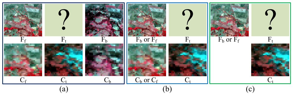
Existing STF models can be broadly classified into three categories according to prior data employed. The first category generates fine-resolution imagery for the prediction date using two pairs of coarse-fine resolution images at prior dates and the coarse-resolution image of the prediction date, as illustrated in Figure 1a. The second category generates fine-resolution images for the prediction date by using one pair of coarse-fine resolution images from the prior date and the coarse-resolution image of the prediction date, as shown in Figure 1b. The third category generates fine-resolution images for the prediction date by employing the fine-resolution image at the prior date and the coarse-resolution image of the prediction date, as shown in Figure 1c. In recent years, STF technologies have developed rapidly and can be broadly categorized into weighted-based STF methods, unmixing-based STF approaches, hybrid STF methods, and learning-based STF models [9,10,11,12].

Among weighted-based STF methods, the core distinction among extensive variants lies in the specific strategies for similar pixel identification and weight calculation. A spatial and temporal adaptive reflectance fusion model (STARFM) [13] pioneered the STF of RSIs. STARFM utilizes the data strategy in Figure 1a to fuse Landsat and MODIS images, generating daily Landsat images. STARFM first employs a sliding window on the Landsat image at the prior date to identify pixels similar to the central pixel and subsequently calculates the weights of similar pixels between Landsat and MODIS to derive the predicted value. The prediction accuracy of STARFM is constrained when mapping targets with dimensions smaller than the coarse-resolution pixel size, and it exhibits poor applicability in complex heterogeneous landscapes. To further improve prediction accuracy, the enhanced STARFM (ESTARFM) [14] was developed. ESTARFM leverages the data strategy illustrated in Figure 1b to fuse Landsat and MODIS images, generating Landsat products at the prediction date. ESTARFM searches for similar pixels using all bands, calculates weights based on spectral similarity, and introduces different conversion coefficients, thereby enhancing prediction accuracy in heterogeneous scenes. However, predicting scenes with shape changes remains challenging, resulting in blurred boundaries. To address the limitation that cloud-free fine-resolution prior images rarely have close temporal proximity to the prediction date and even exhibit intense temporal dynamics, a three-step method (Fit-FC)  [15] is developed, consisting of regression model fitting, spatial filtering, and residual compensation. Fit-FC leverages the data strategy in Figure 1a to generate daily Sentinel-2 products and achieves superior performance in scenarios with dramatic temporal variations. Overall, weighting-based STF methods are simple and easy to implement. However, these methods rely heavily on high-quality prior data, making it difficult to achieve reliable and accurate predictions for scenes with massive abrupt changes. Furthermore, built on the fundamental assumption that temporal changes in coarse-resolution images are consistent with those in fine-resolution images, these methods face considerable challenges when predicting scenes with dramatic temporal variations over a short period or large-scale scenes.

Unmixing-based STF methods predict fine-resolution images by performing spectral unmixing on coarse-resolution images. LSUSDFM [16] devised a linear spectral unmixing-based STF model. LSUSDFM reconstructs the fused image based on the endmember spectral signals and the corresponding abundance maps of the coarse-resolution image. LSUSDFM only requires a prior fine-resolution image and a target coarse-resolution image and effectively mitigates the blocking artifacts. LSUSDFM can predict phenological changes and fuse multisource RSIs, but the prediction performance is suboptimal in areas with land cover type changes. To address the issue that multitemporal RSIs always exhibit substantial differences, leading to large increments and significant uncertainty in downscaling, a virtual image pair-based STF (VIPSTF) [17] method was proposed, and further, a VIPSTF variant integrated with spatial unmixing was investigated, where the virtual image pairs are generated from prior Landsat-MODIS image pairs. VIPSTF is a framework that can be applied to and enhance existing weighted-based and unmixing-based methods, achieving notable prediction performance for longer time intervals and multiple image fusion while exhibiting higher computational efficiency. To address block artifacts via spatial continuity constraints, a spatial unmixing method with block removal (SU-BR) [18] establishes a flexible framework, improving prediction accuracy in heterogeneous landscapes, homogeneous regions, and areas with land cover changes. Overall, unmixing-based STF methods feature the merits of straightforward implementation, flexible operability, and reconstruction of abrupt changes and details to a certain extent. Nevertheless, these methods are generally built on the assumption of invariant land cover types. Coarse-resolution images fail to accurately unmix every land cover information, leading to poor unmixing performance in scenes with diverse land cover categories and resulting in block artifacts induced by endmember classification. Moreover, predicting abrupt changes in land cover types remains challenging.

Among learning-based models, deep learning (DL)-driven STF has undergone rapid and extensive development [19].

In terms of the generative adversarial network (GAN), GAN-STFM [20] implemented an STF model based on a conditional GAN employing the data strategy in Figure 1c. GAN-STFM overcomes the temporal limitations of prior images and enhances STF applicability. HPLTS-GAN [21] designed adaptive spatial distribution transformation, multi-level feature extraction, and cross-scale attention feature fusion and reconstruction to improve the spatiotemporal consistency, feature utilization, and fusion performance.

For convolution and attention mechanism-driven STF models, SwinSTFM [22] implemented an STF model based on the Swin-Transformer and linear spectral mixture. Since high-quality image pairs are difficult to obtain, the SwinSTFM model requires data augmentation or pre-trained models to prevent overfitting. CTSTFM [23] constructed an STF model based on the convolution-Transformer, which designed a multikernel convolution-Transformer encoder, a cross-fusion module, and a convolution-based compression decoder to enhance feature extraction and fusion capability. DGFANet [24] constructed a deformable global–local feature alignment network for unpaired STF, which adopts a hybrid CNN-Transformer architecture for global–local feature alignment for enhancing texture and semantic details. Furthermore, a color consistency loss function is designed to reduce color loss and preserve texture information. AGSDF [25] implemented a multiscale attention-guided deep optimization network for STF using the data strategy in Figure 1b. AGSDF employs a physical attention mechanism to mitigate the impact of climate change in time-series RSIs and performs continuous STF across multiple scales to enhance the STF robustness. LCCINet [26] developed a land cover change inpainting network for STF adopting the data strategy in Figure 1b. LCCINet designs a change detection module to generate a change mask, then modulates the features of the high-spatial-resolution image via a feature mask modulator. A feature fusion encoder focuses on aggregating the unchanged features, while image inpainting modules progressively reconstruct the fine-resolution image using the change mask and contextual cues. ECPW-STFN [27] implemented an enhanced cross-pairing wavelet STF network leveraging the data strategy in Figure 1c. ECPW-STFN conducts independent training for high-frequency and low-frequency components, enabling more accurate extraction of multilevel hierarchical features. Furthermore, a composite loss function incorporating wavelet loss is designed to preserve details. CIG-STF [28] integrates change detection and STF into a unified framework, capturing land cover changes to guide and assist fusion, and designs a dynamic decay loss function using change information to further boost the prediction accuracy. RealFusion [29] implemented a reliable STF framework by integrating diverse inputs, a task-decoupled architecture, advanced inpainting and fusion networks, an adaptive training strategy, and a comprehensive accuracy evaluation system. RealFusion robustly and accurately reconstructs areas with drastic land surface changes and low-quality images. A three-branch convolutional neural network (CNN) for STF [30] is devised using the strategy illustrated in Figure 1a, which incorporates a dual-stream spatial network and a temporal difference network. The spatial branch integrates spatiotemporal adaptive modulation to boost feature discriminability, while the temporal branch leverages lightweight depthwise separable convolutions to efficiently capture dynamic changes.

Regarding diffusion models, given that the sensor and scaling errors may follow a Gaussian noise distribution, CDMSTF [31] implemented a conditional diffusion model-based STF algorithm to characterize stochastic noise. CDMSTF enables finer preservation of details and adaptation to phenological abrupt events. STFDiff [32] presented an STF diffusion model, which iteratively predicts noise via a dual-stream Unet conditional noise predictor driven by Gaussian noise and prior date images, generating fine-resolution images that retain details and temporal dynamics. GCM-PDA [33] introduced a generative compensation model with progressive difference attenuation for STF. GCM-PDA tackles large-scale differences via progressive fusion, alleviates radiation biases using domain adaptation, and achieves spatial-spectral compensation utilizing diffusion and style transfer techniques. GCM-PDA overcomes the limitation of insufficient prior images and displays robust performance under diverse conditions.

STF methods based on CNNs, GANs, Transformers, and diffusion have rapidly advanced, demonstrating highly promising performance. However, there remain many specificities in STF that require further consideration. The architecture, feature extraction, fusion strategy, and loss function of DL models need to be tailored for STF to enhance the generalization capability of STF models across different scenarios and prediction ability for abrupt changes.

Hybrid STF methods integrate the strengths of multiple STF solutions to achieve superior fusion accuracy. FSDAF [34] realized a flexible STF method based on spectral unmixing analysis and thin plate spline interpolation. FSDAF is suitable for heterogeneous landscapes and enables more accurate prediction of both gradual changes and land cover type changes. Subsequently, improved versions were developed, including improved FSDAF (IFSDAF) [35], FSDAF 2.0 [36], cuFSDAF [37], and robust FSDAF [38], enhancing the STF accuracy or optimizing the computational efficiency. LiSTF [39] performed reconstruction directly from MODIS-like images using a linear regression STF strategy. LiSTF effectively reduces uncertainty errors of the model and better preserves fine-grained spatial details. The CycleGAN is introduced in STF [40] to simulate the changes between two fine-resolution images and generate a batch of synthetic fine-resolution images. Subsequently, the coarse-resolution image at the target date is leveraged to screen valid synthetic images, which are further enhanced via wavelet transform. Ultimately, the FSDAF is employed to complete the final STF. Although this approach improves STF performance, the randomly synthetic images may introduce significant deviations, resulting in fewer viable images, and multiple GANs are relatively time-consuming. FastVSDF [41] achieved a fast FSDAF, which integrates a fast and robust change classification strategy and an intra-class Gaussian weighting function to accelerate computation and improve fidelity. Furthermore, a fast guided filter is employed to eliminate the blocking artifacts in the global residuals. W-STFTCR [42] developed a weighted STF approach based on tensor collaborative representation, which incorporates collaborative representation constraints into the tensor decomposition framework to prevent overfitting and enhance STF robustness. Meanwhile, a superpixel segmentation strategy is adopted to construct block dictionaries and perform clustering. Furthermore, the normalized difference vegetation index and joint information entropy are introduced to improve the physical interpretability and STF accuracy. Hybrid STF methods can integrate the advantages of distinct STF solutions to improve the prediction accuracy of land surface changes and enhance cross-scenario generalization capability. However, the complexity of the methods also increases, which limits their widespread applicability. Overall, hybrid STF methods are suitable for scenarios with stringent requirements for fusion accuracy and non-stringent constraints on computational complexity and hardware resources.

In summary, current DL-based STF models have achieved promising prediction performance, particularly excelling in scenarios involving gradual phenological changes. Nevertheless, there remains substantial room for improvement in prediction accuracy for scenarios with abrupt changes over short time periods, long temporal intervals, and land cover type conversions. Although most STF methods based on the data strategy illustrated in Figure 1a achieve superior accuracy to those of the other two strategies, it is rare to obtain well-aligned paired, high-quality, and cloud-free coarse- and fine-resolution RSIs for actual observations of dynamic scenarios, which hinders the STF application. STF approaches based on the data strategy in Figure 1c utilize only the coarse-resolution image at the prediction time. The vast resolution gap between coarse- and fine-resolution images greatly limits the available information, making it challenging to effectively leverage prior spatiotemporal variations. Moreover, there exist notable sensor-induced imaging discrepancies between the coarse- and fine-resolution images. Based on the data strategy in Figure 1b, spatiotemporal difference information between the prior time and the prediction time can be captured. However, the fusion results are susceptible to interference from the prior information.

To address the aforementioned critical limitations, a temporal-variation-resistant bidirectional convolution-Transformer GAN (TRB-GAN) for STF of RSIs is proposed. Extensive ablation and comparative experiments are conducted on widely used public datasets, CIA and LGC. The results demonstrate the superior STF capability and time-varying robustness of the proposed TRB-GAN model for the CIA and LGC data. The main contributions are as follows:

(1)

TRB-GAN framework for temporal-variation-resistant STF: A TRB-GAN is proposed to improve the predictive robustness for time-varying information and STF capability, consisting of a temporal-variation-resistant bidirectional convolution-Transformer generator (TRBG) and a multiresolution input convolution-Transformer discriminator (MICTD).

(2)

Bidirectional time-varying encoder for enhanced dynamic feature modeling: The TRBG devises a temporal-variation-resistant bidirectional encoder to bidirectionally capture local–global features of both prior and arbitrary time-varying information, enhancing the representation capability for time-varying information and the prediction robustness of dynamic changes.

(3)

Dual-guided triple-attention fusion decoder (DTAFD) for heterogeneous feature aggregation: The TRBG designs a DTAFD, incorporating dual-guided cross convolution-attention fusion and decision attention fusion, which dynamically computes the correlations among spectral, spatial, and time-varying information to aggregate heterogeneous features and adaptively performs stepwise weighting, thereby mitigating the discrepancies caused by heterogeneous imaging mechanisms and significant resolution differences.

(4)

MICTD for fine-grained image reconstruction: A MICTD with multiresolution inputs and deep supervision are introduced to adversarially learn the local–global structures and spectral information across different resolutions and provide feedback to the TRBG to produce finer images.

2. Methodology

2.1. Motivation and Model Framework

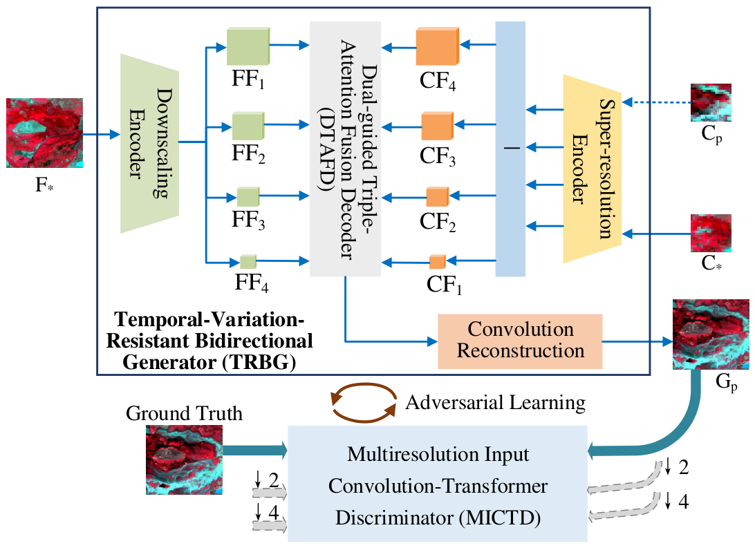
To tackle the critical bottlenecks of existing STF frameworks, including the huge resolution gap between fine- and coarse-resolution images, severe performance degradation induced by prior data and complex time-varying land surface changes, and the limited effective information available in coarse-resolution images, the TRB-GAN is proposed. The overall framework of the proposed TRB-GAN is illustrated in Figure 2, which comprises a TRBG and a MICTD, capturing and modeling complex time-varying land surface changes and fine-grained details from prior observations via adversarial learning.

First, existing STF models may exhibit detail and spectral distortions in predictions for areas with intense temporal changes when there is a significant temporal variation discrepancy between the test data and the training samples or abrupt scenario changes. Consequently, the ability to capture land surface changes deteriorates, resulting in unreliable predictions of land cover changes. To address this critical challenge, improving the adaptive learning capabilities of the model regarding variations across arbitrary time intervals is essential to boost robustness and prediction accuracy under complex time-varying scenarios. This design effectively reduces the severe STF performance degradation caused by cross-domain data distribution discrepancies and abrupt land cover changes.

Second, the information available in coarse-resolution images is highly restricted. The individual coarse-resolution pixel typically represents a mixture of diverse land cover types, introducing blurring in details and boundaries, which makes it extremely challenging to directly and effectively extract temporal variation information from pure pixels. Furthermore, the mixed pixel exacerbates the phenomenon of dissimilar objects sharing similar spectra and identical objects exhibiting dissimilar spectra, interfering with the capability to accurately differentiate land cover types. The aforementioned challenges are further amplified in regions experiencing rapid or sudden changes, resulting in considerable difficulty in precisely modeling the abrupt and dynamic variations of land cover. To overcome this challenge, super-resolution reconstruction of the temporal change information from coarse-resolution images is performed, progressively enhancing spatial resolution and highlighting the crucial structures and spectra embedded in the coarse-resolution data. As illustrated in Figure 2, a downscaling encoder obtains multiscale features of the fine-resolution image at an arbitrary time (${\mathrm{F}}_{*}$) from a high-to-low resolution; a super-resolution encoder obtains multiscale features of the coarse-resolution image at the arbitrary time (${\mathrm{C}}_{*}$) and the coarse-resolution image at prediction time (${\mathrm{C}}_{\mathrm{p}}$) from low-to-high resolution. The variation features for arbitrary time intervals are then obtained via a subtraction operation.

Finally, since disparate sensors exhibit differing imaging attributes arising from their distinct imaging mechanisms, a DTAFD is proposed to reduce sensor discrepancies and effectively aggregate complementary information from the dual sources. Guided by dual semantic features derived from prior fine-grained spatial details and dynamic time-varying change information, the DTAFD aggregates complementary information regarding spatial structure and semantic content via parallel attention streams. To alleviate uncertainties and biases introduced by a single large-scale resolution enhancement, the DTAFD employs a small-scale ratio and multistage decision attention fusion to progressively improve resolution and reconstruct intermediate-resolution images. Furthermore, a MICTD is devised to hierarchically and adversarially learn local–global multiresolution details and temporal change information, thereby preserving the consistency of spatiotemporal evolution.

2.2. Temporal-Variation-Resistant Bidirectional Generator

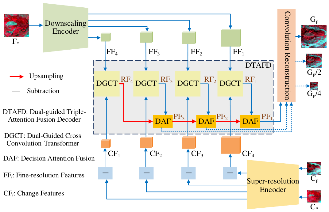
A temporal-variation-resistant bidirectional convolution-Transformer generator (TRBG) is proposed, presented in Figure 3. The TRBG comprises a downscaling encoder, a super-resolution encoder, a DTAFD, and a reconstruction unit. The downscaling encoder and super-resolution encoder capture multiscale local–global prior features and temporal variation features. The DTAFD integrates a dual-guided cross convolution-Transformer with decision attention fusion, progressively aggregating complementary information from spatial structure and semantic content. The reconstruction unit is implemented to reconstruct the fused feature maps and yield desired-resolution images.

2.2.1. Temporal-Variation-Resistant Bidirectional Encoder

Existing STF models are prone to producing predictions with severe detail and spectral distortions in regions with noticeable temporal variations or abrupt scene changes. Consequently, the capability to capture authentic land surface changes is decreased, preventing accurate prediction of land cover variations. To address this critical challenge, the proposed approach enhances the adaptive learning capability for change information over arbitrary time intervals by capturing the spatiotemporal differences between the coarse-resolution image at the prediction time (${\mathrm{C}}_{\mathrm{p}}$) and the coarse-resolution image at arbitrary time (${\mathrm{C}}_{*}$). Consequently, the degradation in STF performance caused by differing prior data and sudden scene variations is effectively mitigated.

Moreover, each coarse-resolution pixel inherently represents a mixture of multiple distinct land cover types, which makes it extremely challenging to effectively extract accurate time-varying change signals for different land cover categories. More importantly, the mixed pixel effect significantly exacerbates the well-known spectral confusion problems, i.e., the same spectrum for different objects and different spectra for the same object phenomena, which severely impairs the STF capability to correctly discriminate the land cover types. In regions experiencing dramatic temporal variations or abrupt land cover transitions, these aforementioned limitations are significantly exacerbated, resulting in significant challenges in reliably predicting sudden variations in ground cover. Super-resolution reconstruction on the temporal variation information of coarse-resolution images is performed to progressively enhance the spatial resolution and highlight the critical structures and spectra implicit in the coarse-resolution data.

Recognizing the respective strengths of CNNs in capturing local features and Transformers in establishing long-range dependencies, as demonstrated in Restormer [43], and further inspired by the fact that depthwise convolutional Transformers can decrease computational complexity and are applicable to high-resolution images, a temporal-variation-resistant bidirectional encoder (TRBE) is devised, as illustrated in Figure 3. The TRBE consists of a downscaling encoder and a super-resolution encoder based on convolution-Transformers. The downscaling encoder captures prior features from a high-to-low resolution direction, while the super-resolution encoder captures temporal variation features from a low-to-high resolution direction.

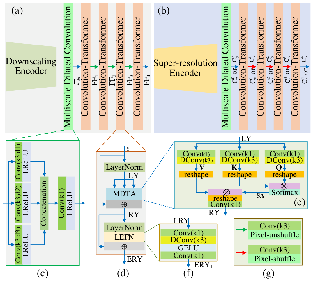
As depicted in Figure 3, the downscaling encoder obtains multiresolution prior features (${\mathrm{FF}}_i$) of the fine-resolution image ${\mathrm{F}}_{*}$ at an arbitrary time from a high-to-low resolution, while the super-resolution encoder captures multiresolution features of the coarse-resolution image at an arbitrary time (${\mathrm{C}}_{*}$) and the coarse-resolution image at the prediction time (${\mathrm{C}}_{\mathrm{p}}$) from a low-to-high resolution. The temporal change features (${\mathrm{CF}}_i$) across arbitrary time intervals are then obtained by element-wise subtraction between the corresponding multiresolution features of ${\mathrm{C}}_{*}$ and ${\mathrm{C}}_{\mathrm{p}}$. The architectures of the downscaling encoder and the super-resolution encoder are presented in Figure 4a,b. The downscaling encoder consists of multiscale dilated convolutions, convolution-Transformers, and progressive downsampling layers, while the super-resolution encoder comprises multiscale dilated convolutions, convolution-Transformers, and progressive upsampling layers.

The multiscale dilated convolution module is designed to extract multiscale local features representing low-level semantics from ${\mathrm{F}}_{*}$, ${\mathrm{C}}_{*}$, and ${\mathrm{C}}_{\mathrm{p}}$ images. As illustrated in Figure 4c, convolutions with dilation rates of 1, 2, and 3 are executed in parallel to acquire multiscale features from ${\mathrm{F}}_{*}$, ${\mathrm{C}}_{*}$, and ${\mathrm{C}}_{\mathrm{p}}$ images. The multiscale features are then channel-wise concatenated, followed by a 1 × 1 convolution for preliminary fusion and adjustment of the number of channels. Conv(k3,d1) indicates a convolution with a kernel size of 3 × 3 and a dilation rate of 1. The implementation of the multiscale dilated convolution module for extracting low-level semantic features is expressed as Equations (1)–(3).

$${\mathrm{F}}_{*}^0=f_{\mathrm{cvl}}^1\left(f_{\mathrm{cat}}\left(f_{\mathrm{lrelu}}\left(f_{\mathrm{cv}}^{3,d_1}\left({\mathrm{F}}_{*}\right),f_{\mathrm{cv}}^{3,d_2}\left({\mathrm{F}}_{*}\right),f_{\mathrm{cv}}^{3,d_3}\left({\mathrm{F}}_{*}\right)\right)\right)\right)$$

(1)

$${\mathrm{C}}_{*}^0=f_{\mathrm{cvl}}^1\left(f_{\mathrm{cat}}\left(f_{\mathrm{lrelu}}\left(f_{\mathrm{cv}}^{3,d_1}\left({\mathrm{C}}_{*}\right),f_{\mathrm{cv}}^{3,d_2}\left({\mathrm{C}}_{*}\right),f_{\mathrm{cv}}^{3,d_3}\left({\mathrm{C}}_{*}\right)\right)\right)\right)$$

(2)

$${\mathrm{C}}_{\mathrm{p}}^0=f_{\mathrm{cvl}}^1\left(f_{\mathrm{cat}}\left(f_{\mathrm{lrelu}}\left(f_{\mathrm{cv}}^{3,d_1}\left({\mathrm{C}}_{\mathrm{p}}\right),f_{\mathrm{cv}}^{3,d_2}\left({\mathrm{C}}_{\mathrm{p}}\right),f_{\mathrm{cv}}^{3,d_3}\left({\mathrm{C}}_{\mathrm{p}}\right)\right)\right)\right)$$

(3)

where ${\mathrm{F}}_{*}^0$, ${\mathrm{C}}_{*}^0$, and ${\mathrm{C}}_{\mathrm{p}}^0$ denote the low-level semantic features extracted from ${\mathrm{F}}_{*}$, ${\mathrm{C}}_{*}$, and ${\mathrm{C}}_{\mathrm{p}}$; $f_{\mathrm{cv}}^{3,d_1}(·)$, $f_{\mathrm{cv}}^{3,d_2}(·)$, $f_{\mathrm{cv}}^{3,d_3}(·)$ represent the dilated convolution operations with a kernel size of 3 and dilation rates of 1, 2, and 3; $f_{\mathrm{lrelu}}(·)$ signifies the leaky ReLU (LReLU) function; $f_{\mathrm{cat}}(·)$ refers to the concatenation operation along the channel dimension; and $f_{\mathrm{cvl}}^1(·)$ indicates a convolution operation with a kernel size of 1 followed by the LReLU.

To effectively capture high-level hierarchical multiscale prior details and temporal variation information, a multiresolution feature extraction module integrating convolution-Transformers with downsampling or upsampling is introduced. As depicted in Figure 4a,b, the downscaling encoder consists of four convolution-Transformer blocks and three downsampling modules, extracting four hierarchical prior detail semantic features ${\mathrm{FF}}_i$ at distinct resolutions along the high-to-low resolution manner. The super-resolution encoder comprises four convolution-Transformer blocks and three upsampling modules, capturing four hierarchical semantic features at distinct resolutions from ${\mathrm{C}}_{*}$ and ${\mathrm{C}}_{\mathrm{p}}$ along the low-to-high resolution manner, and then obtaining temporal variation semantic features ${\mathrm{CF}}_i$ across arbitrary time intervals via the element-wise subtraction. The architectures of the convolution-Transformer, downsampling, and upsampling are illustrated in Figure 4d,g. The downsampling and upsampling operations are executed via the pixel-unshuffle and pixel-shuffle operations. Conv(k3) denotes a 3 × 3 convolution to adjust the number of channels. The implementation of high-level multiresolution semantic features for ${\mathrm{F}}_{*}$, ${\mathrm{C}}_{*}$, and ${\mathrm{C}}_{\mathrm{p}}$ is described by Equations (4)–(6), and the temporal variation semantic features are obtained as expressed in Equation (7).

$$\left\{\begin{array}{c}\mathrm{F}{\mathrm{F}}_1=f_{\mathrm{CT}}\left({\mathrm{F}}_{*}^0\right)\hfill \\ \mathrm{F}{\mathrm{F}}_i=f_{\mathrm{CT}}\left(f_{\mathrm{ds}}\left(\mathrm{F}{\mathrm{F}}_{i-1}\right)\right)\hspace{1em}i=2,\cdots ,4\hfill \end{array}\right.$$

(4)

$$\left\{\begin{array}{c}{\mathrm{C}}_{*}^1=f_{\mathrm{CT}}\left({\mathrm{C}}_{*}^0\right)\hfill \\ {\mathrm{C}}_{*}^i=f_{\mathrm{CT}}\left(f_{\mathrm{us}}\left({\mathrm{C}}_{*}^{i-1}\right)\right)\hspace{1em}i=2,\cdots ,4\hfill \end{array}\right.$$

(5)

$$\left\{\begin{array}{c}{\mathrm{C}}_{\mathrm{p}}^1=f_{\mathrm{CT}}\left({\mathrm{C}}_{\mathrm{p}}^0\right)\hfill \\ {\mathrm{C}}_{\mathrm{p}}^i=f_{\mathrm{CT}}\left(f_{\mathrm{us}}\left({\mathrm{C}}_{\mathrm{p}}^{i-1}\right)\right)\hspace{1em}i=2,\cdots ,4\hfill \end{array}\right.$$

(6)

$$\mathrm{C}{\mathrm{F}}_i={\mathrm{C}}_{\mathrm{p}}^i-{\mathrm{C}}_{*}^i\hspace{1em}i=1,\cdots ,4$$

(7)

where ${\mathrm{FF}}_i$ and $\mathrm{C}{\mathrm{F}}_i\left(i=1,\cdots ,4\right)$ denote the extracted prior detail semantic features and temporal variation semantic features at the i-th resolution; ${\mathrm{C}}_{*}^i$ and ${\mathrm{C}}_{\mathrm{p}}^i\left(i=1,\cdots ,4\right)$ represent the i-th resolution semantic features of ${\mathrm{C}}_{*}$ and ${\mathrm{C}}_{\mathrm{p}}$; $f_{\mathrm{CT}}(·)$ denotes the function of the convolution-Transformer; and $f_{\mathrm{ds}}(·)$ and $f_{\mathrm{us}}(·)$ represent downsampling and upsampling operations.

Constrained by the local receptive fields of CNNs, global structures are often neglected, resulting in insufficient reconstruction of high-quality images. Standard self-attention is capable of capturing long-range dependencies but suffers from high computational cost [43]. Therefore, a multi-head depthwise convolutional transposed attention (MDTA) module and a locally enhanced feed-forward network (LEFN) are introduced to collaboratively capture long-range dependencies, enhance local details, and reduce computational overhead. As illustrated in Figure 4d, the convolution-Transformer comprises layer normalization, the MDTA module, the LEFN, and residual connections.

The architecture of the MDTA module is illustrated in Figure 4e. The input image Y is normalized by layer normalization to obtain LY. Then, a 1 × 1 convolution layer aggregates pixel-wise cross-channel context, and a 3 × 3 depthwise convolution encodes channel-separated spatial context and generates query (Q), key (K), and value (V). The self-attention map SA is computed by reshaping, dot product, and Softmax operations on Q and K. V is reshaped and multiplied with SA, followed by another reshaping and convolution to produce the calibrated feature $\mathrm{R}{\mathrm{Y}}_1$. Finally, $\mathrm{R}{\mathrm{Y}}_1$ is added to the input Y to obtain the local–global feature RY. The implementation process is expressed as Equations (8)–(10).

$$\mathrm{LY}=f_{\mathrm{LN}}\left(\mathrm{Y}\right)$$

(8)

$$\left[\mathrm{Q},\mathrm{K},\mathrm{V}\right]=\left[f_{\mathrm{Q}}^{\mathrm{dwc},3}\left(f_{\mathrm{Q}}^{\mathrm{cv},1}\left(\mathrm{LY}\right)\right),f_{\mathrm{K}}^{\mathrm{dwc},3}\left(f_{\mathrm{K}}^{\mathrm{cv},1}\left(\mathrm{LY}\right)\right)\right.,\left.f_{\mathrm{V}}^{\mathrm{dwc},3}\left(f_{\mathrm{V}}^{\mathrm{cv},1}\left(\mathrm{LY}\right)\right)\right]$$

(9)

$$\mathrm{RY}=\mathrm{Y}+f_{\mathrm{cv}}^1\left(f_r\left(f_r\left(\mathrm{V}\right)·f_{\mathrm{Soft}}\left(f_r\left(\mathrm{K}\right)·f_r\left(\mathrm{Q}\right)/\alpha \right)\right)\right)$$

(10)

where Y, LY, and RY denote the input feature, layer-normalized feature, and the local–global feature corrected by MDTA; $f_{\mathrm{LN}}$ represents the layer normalization operation; $f_{\mathrm{Q}}^{\mathrm{cv},1}$ and $f_{\mathrm{Q}}^{\mathrm{dwc},3}$ are the 1 × 1 convolution and 3 × 3 depthwise convolution that generate Q; $f_{\mathrm{K}}^{\mathrm{cv},1}$ and $f_{\mathrm{K}}^{\mathrm{dwc},3}$ are the 1 × 1 convolution and 3 × 3 depthwise convolution for generating K; $f_{\mathrm{V}}^{\mathrm{cv},1}$ and $f_{\mathrm{V}}^{\mathrm{dwc},3}$ are the 1 × 1 convolution and 3 × 3 depthwise convolution to produce V; $\alpha$ is a learnable parameter for amplitude adjustment; $f_r(·)$ refers to the reshaping operation; $f_{\mathrm{Soft}}(·)$ signifies the Softmax operation; and $f_{\mathrm{cv}}^1(·)$ indicates a 1 × 1 convolution operation.

As depicted in Figure 4d, RY is passed through layer normalization to the LEFN, which enhances the local context, and the enhanced feature ERY is produced via a residual connection. The structure of LEFN is presented in Figure 4f, and the implementation procedure is formulated as Equation (11).

$$\mathrm{ERY}=f_{\mathrm{cv}}^1\left(f_{\mathrm{GELU}}\left(f_{\mathrm{dwc}}^3\left(f_{\mathrm{cv}}^1\left(f_{\mathrm{LN}}\left(\mathrm{RY}\right)\right)\right)\right)\right)+\mathrm{RY}$$

(11)

where $f_{\mathrm{GELU}}$ is the Gaussian error linear unit (GELU) function, and $f_{\mathrm{dwc}}^3(·)$ represents the 3 × 3 depthwise convolution operation.

With the collaboration of the MDTA and LEFN, the convolution-Transformer simultaneously captures fine-grained local features and models long-range global contextual dependencies across different regions, thereby facilitating the reconstruction of high-quality RSIs.

2.2.2. Dual-Guided Triple-Attention Fusion Decoder

To mitigate the effects of disparity in diverse imaging mechanisms and vast resolution gaps and enhance the ability to perceive and predict dynamic change scenarios, a DTAFD is proposed, as depicted in Figure 3. The DTAFD designs a dual-guided cross convolution-Transformer (DGCT), which consists of prior semantic feature-guided cross-attention fusion and temporal variation information-guided cross-attention fusion to aggregate heterogeneous prior information and temporal variation information, dynamically modeling the correlations between spectral and spatial features. Furthermore, the DTAFD introduces a decision attention fusion mechanism to perform high-level adaptive weighting and integration of the hierarchical cross-fusion results at different resolutions. The implementation of the DTAFD can be divided into the following two core modules.

(1) Dual-Guided Cross Convolution-Transformer

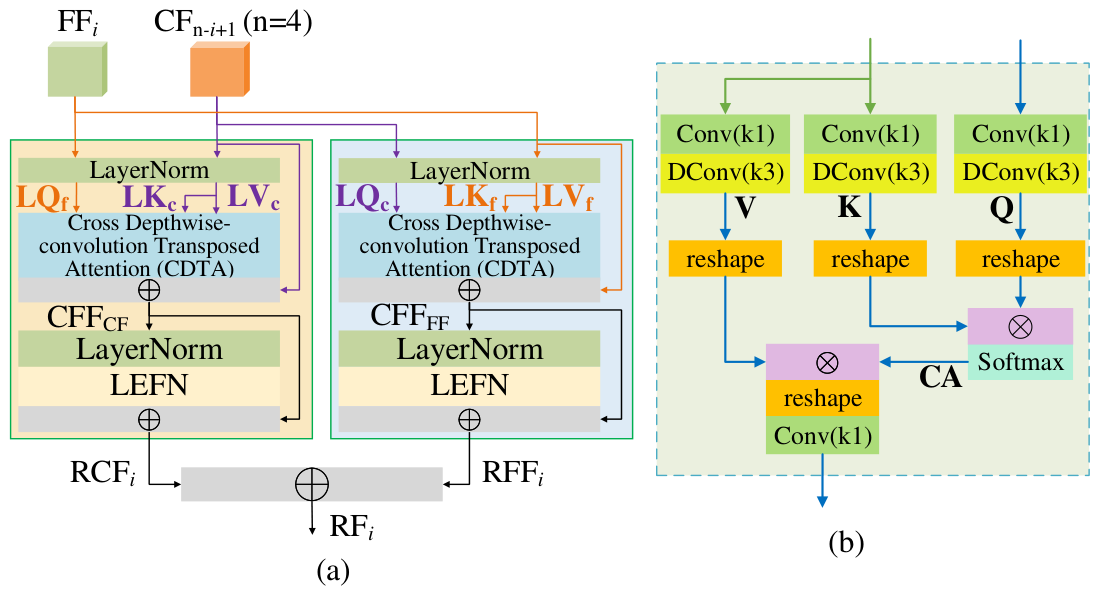
As displayed in Figure 3, to aggregate heterogeneous prior information and temporal change information, a DGCT is devised to fuse the local–global prior semantic features $\mathrm{F}{\mathrm{F}}_i\left(i=4,3,2,1\right)$ and temporal-change semantic features $\mathrm{C}{\mathrm{F}}_{4-i+1}\left(i=4,3,2,1\right)$ at different resolutions to generate preliminary local–global cross-fusion features $\mathrm{R}{\mathrm{F}}_i$. The architecture of DGCT is shown in Figure 5a, which includes prior semantic feature-guided cross-attention fusion and temporal-change semantic feature-guided cross-attention fusion. Both comprise layer normalization, cross depthwise-convolution transposed attention (CDTA), LEFN, and residual connections.

The prior semantic feature-guided cross-attention fusion first performs layer normalization on $\mathrm{F}{\mathrm{F}}_i\left(i=4,3,2,1\right)$ and $\mathrm{C}{\mathrm{F}}_{4-i+1}\left(i=4,3,2,1\right)$ to obtain normalized features $\mathrm{L}{\mathrm{Q}}_{\mathrm{c}}$, $\mathrm{L}{\mathrm{K}}_{\mathrm{f}}$, and $\mathrm{L}{\mathrm{V}}_{\mathrm{f}}$. Subsequently, the CDTA performs cross-attention fusion to produce the corrected features, which are then added to $\mathrm{F}{\mathrm{F}}_i$ to obtain the preliminary cross-attention fusion feature ${\mathrm{CFF}}_{\mathrm{FF}}$. Finally, the ${\mathrm{CFF}}_{\mathrm{FF}}$ is fed into the LEFN to further enhance local information, yielding the refined cross-fusion feature ${\mathrm{RFF}}_i$. The implementation process is expressed as Equations (12)–(15).

$$\left\{\begin{array}{c}\mathrm{L}{\mathrm{Q}}_{\mathrm{c}}=f_{\mathrm{LN}}\left(\mathrm{C}{\mathrm{F}}_{4-i+1}\right)\hfill \\ \mathrm{L}{\mathrm{K}}_{\mathrm{f}}=\mathrm{L}{\mathrm{V}}_{\mathrm{f}}=f_{\mathrm{LN}}\left(\mathrm{F}{\mathrm{F}}_i\right)\hfill \end{array}\right.$$

(12)

$$\left[\mathrm{Q},\mathrm{K},\mathrm{V}\right]=\left[f_{\mathrm{Q}}^{\mathrm{dwc},3}\left(f_{\mathrm{Q}}^{\mathrm{cv},1}\left(\mathrm{L}{\mathrm{Q}}_{\mathrm{c}}\right)\right),f_{\mathrm{K}}^{\mathrm{dwc},3}\left(f_{\mathrm{K}}^{\mathrm{cv},1}\left(\mathrm{L}{\mathrm{K}}_{\mathrm{f}}\right)\right)\right.,\left.f_{\mathrm{V}}^{\mathrm{dwc},3}\left(f_{\mathrm{V}}^{\mathrm{cv},1}\left(\mathrm{L}{\mathrm{V}}_{\mathrm{f}}\right)\right)\right]$$

(13)

$${\mathrm{CFF}}_{\mathrm{FF}}={\mathrm{FF}}_i+f_{\mathrm{cv}}^1\left(f_r\left(f_r\left(\mathrm{V}\right)·f_{\mathrm{Soft}}\left(f_r\left(\mathrm{K}\right)·f_r\left(\mathrm{Q}\right)/\alpha \right)\right)\right)$$

(14)

$${\mathrm{RFF}}_i={\mathrm{CFF}}_{\mathrm{FF}}+f_{\mathrm{LEFN}}\left(f_{\mathrm{LN}}\left(\mathrm{CF}{\mathrm{F}}_{\mathrm{FF}}\right)\right)i=4,3,2,1$$

(15)

where $\mathrm{L}{\mathrm{Q}}_{\mathrm{c}}$ denotes the normalized feature of $\mathrm{C}{\mathrm{F}}_{4-i+1}$ used to generate the Q; $\mathrm{L}{\mathrm{K}}_{\mathrm{f}}$ and $\mathrm{L}{\mathrm{V}}_{\mathrm{f}}$ represent the normalized features of $\mathrm{F}{\mathrm{F}}_i$ used to produce K and V; ${\mathrm{CFF}}_{\mathrm{FF}}$ indicates the preliminary cross-attention fusion feature generated under the guidance of $\mathrm{F}{\mathrm{F}}_i$; and ${\mathrm{RFF}}_i$ denotes the enhanced local–global cross-fusion feature generated under the guidance of $\mathrm{F}{\mathrm{F}}_i$.

The implementation of CDTA is illustrated in Figure 5b. The key difference from MDTA is the method of obtaining Q, K and V. Specifically, in the prior semantic feature-guided cross-attention fusion, Q in CDTA is derived from the temporal change feature $\mathrm{C}{\mathrm{F}}_{4-i+1}\left(i=4,3,2,1\right)$ by applying a 1 × 1 pointwise convolution followed by a 3 × 3 depthwise convolution, and K and V are generated by mapping $\mathrm{F}{\mathrm{F}}_i\left(i=4,3,2,1\right)$ via 1 × 1 convolution and 3 × 3 depthwise convolution. The realization process is expressed as Equation (13).

Analogously, the temporal-change semantic feature-guided cross-attention fusion first performs layer normalization on $\mathrm{F}{\mathrm{F}}_i$ and $\mathrm{C}{\mathrm{F}}_{4-i+1}\left(i=4,3,2,1\right)$ to obtain normalized features $\mathrm{L}{\mathrm{Q}}_{\mathrm{f}}$, $\mathrm{L}{\mathrm{K}}_{\mathrm{c}}$, and $\mathrm{L}{\mathrm{V}}_{\mathrm{c}}$. Subsequently, the CDTA performs cross-attention fusion to produce the calibrated feature, which is then added to the temporal change feature $\mathrm{C}{\mathrm{F}}_{4-i+1}$ to obtain the preliminary cross-fusion feature ${\mathrm{CFF}}_{\mathrm{CF}}$. Finally, ${\mathrm{CFF}}_{\mathrm{CF}}$ is passed to LEFN for further local enhancement to yield the refined cross-fusion feature $\mathrm{RC}{\mathrm{F}}_i$. The realization process is expressed as Equations (16)–(19). In the CDTA, Q is derived from $\mathrm{F}{\mathrm{F}}_i\left(i=4,3,2,1\right)$ via a 1×1 convolution and a 3 × 3 depthwise convolution. Correspondingly, K and V are obtained by mapping $\mathrm{C}{\mathrm{F}}_{4-i+1}\left(i=4,3,2,1\right)$ via a 1 × 1 convolution and a 3 × 3 depthwise convolution. The implementation is expressed as Equation (17).

$$\left\{\begin{array}{c}\mathrm{L}{\mathrm{Q}}_{\mathrm{f}}=f_{\mathrm{LN}}\left(\mathrm{F}{\mathrm{F}}_i\right)\hfill \\ \mathrm{L}{\mathrm{K}}_{\mathrm{c}}=\mathrm{L}{\mathrm{V}}_{\mathrm{c}}=f_{\mathrm{LN}}\left(\mathrm{C}{\mathrm{F}}_{4-i+1}\right)\hfill \end{array}\right.$$

(16)

$$\left[\mathrm{Q},\mathrm{K},\mathrm{V}\right]=\left[f_{\mathrm{Q}}^{\mathrm{dwc},3}\left(f_{\mathrm{Q}}^{\mathrm{cv},1}\left(\mathrm{L}{\mathrm{Q}}_{\mathrm{f}}\right)\right),f_{\mathrm{K}}^{\mathrm{dwc},3}\left(f_{\mathrm{K}}^{\mathrm{cv},1}\left(\mathrm{L}{\mathrm{K}}_{\mathrm{c}}\right)\right),\right.\left.f_{\mathrm{V}}^{\mathrm{dwc},3}\left(f_{\mathrm{V}}^{\mathrm{cv},1}\left(\mathrm{L}{\mathrm{V}}_{\mathrm{c}}\right)\right)\right]$$

(17)

$$\mathrm{CF}{\mathrm{F}}_{\mathrm{CF}}=\mathrm{C}{\mathrm{F}}_{4-i+1}+f_{\mathrm{cv}}^1\left(f_r\left(f_r\left(\mathrm{V}\right)·f_{\mathrm{Soft}}\left(f_r\left(\mathrm{K}\right)·f_r\left(\mathrm{Q}\right)/\phantom{f_r\left(\mathrm{Q}\right)\alpha }\alpha \right)\right)\right)$$

(18)

$$\mathrm{RC}{\mathrm{F}}_i=\mathrm{CF}{\mathrm{F}}_{\mathrm{CF}}+f_{\mathrm{LEFN}}\left(f_{\mathrm{LN}}\left(\mathrm{CF}{\mathrm{F}}_{\mathrm{CF}}\right)\right)i=4,3,2,1$$

(19)

where $\mathrm{L}{\mathrm{Q}}_{\mathrm{f}}$ denotes the normalized feature of $\mathrm{F}{\mathrm{F}}_i$ used to generate the Q; $\mathrm{L}{\mathrm{K}}_{\mathrm{c}}$ and $\mathrm{L}{\mathrm{V}}_{\mathrm{c}}$ represent the normalized features of $\mathrm{C}{\mathrm{F}}_{4-i+1}$ used to produce K and V; $\mathrm{CF}{\mathrm{F}}_{\mathrm{CF}}$ indicates the preliminary cross-attention fusion feature generated under the guidance of $\mathrm{C}{\mathrm{F}}_{4-i+1}$; and $\mathrm{RC}{\mathrm{F}}_i$ denotes the enhanced local–global cross-fusion feature generated under the guidance of $\mathrm{C}{\mathrm{F}}_{4-i+1}$.

Finally, the preliminary local–global cross-fusion feature $\mathrm{R}{\mathrm{F}}_i\left(i=4,3,2,1\right)$ at the i-th resolution is generated by adding ${\mathrm{RFF}}_i$ and $\mathrm{RC}{\mathrm{F}}_i$ obtained from the $\mathrm{F}{\mathrm{F}}_i$-guided and $\mathrm{C}{\mathrm{F}}_{4-i+1}$-guided cross-convolution attention fusion, as shown in Equation (20).

$$\mathrm{R}{\mathrm{F}}_i=\mathrm{RC}{\mathrm{F}}_i+{\mathrm{RFF}}_{i}i=4,3,2,1$$

(20)

(2) Multiresolution Cascaded Decision Attention Fusion

To further reduce the false change information that may arise from the phenomena of “different objects with the same spectrum” and “the same object with different spectra” and improve the fusion accuracy of fine-grained spatial details and spectral characteristics of dynamic changes, a multiresolution cascaded decision attention fusion (MCDAF) module is designed, as shown in Figure 3. The MCDAF hierarchically fuses the cross-fusion result $\mathrm{R}{\mathrm{F}}_i\left(i=3,2,1\right)$ at the i-th resolution and the decision fusion feature $\mathrm{P}{\mathrm{F}}_{i+1}\left(i=3,2,1\right)$ ($\mathrm{P}{\mathrm{F}}_4=\mathrm{R}{\mathrm{F}}_4$) at the (i+1)-th resolution via dual spectral-spatial attention mechanisms, adaptively evaluates and assigns optimal weights for different spectral bands and spatial positions, and generates fused features with better temporal change information and fine-grained prior details. As illustrated in Figure 3, three cascaded DAF perform coarse-to-fine hierarchical decision attention fusion on four-resolution cross-fusion features, yielding the desired-resolution decision-fusion feature, denoted as Equation (21). Subsequently, a reconstruction unit composed of three consecutive convolutions generates the desired-resolution image ${\mathrm{G}}_{\mathrm{p}}$ and two intermediate-resolution images ${\mathrm{G}}_{\mathrm{p}}/\phantom{{\mathrm{G}}_{\mathrm{p}}2}2$ and ${\mathrm{G}}_{\mathrm{p}}/\phantom{{\mathrm{G}}_{\mathrm{p}}4}4$, as described in Equation (22).

$$\left\{\begin{array}{c}\mathrm{P}{\mathrm{F}}_i=f_{\mathrm{DAF}}\left(\mathrm{R}{\mathrm{F}}_i,\mathrm{P}{\mathrm{F}}_{i+1};W_{\mathrm{DAF}}\right)\hspace{1em}i=3,2,1\hfill \\ \mathrm{P}{\mathrm{F}}_4=\mathrm{R}{\mathrm{F}}_4\hfill \end{array}\right.$$

(21)

$${\mathrm{G}}_{\mathrm{p}}/\phantom{{\mathrm{G}}_{\mathrm{p}}{2}^{i-1}}{2}^{i-1}=f_{\mathrm{cv}}^3\left(f_{\mathrm{cvl}}^3\left(f_{\mathrm{cvl}}^3\left(\mathrm{P}{\mathrm{F}}_i\right)\right)\right)\hspace{1em}n=1,2,3$$

(22)

where $f_{\mathrm{DAF}}\left( \right)$ denotes the DAF module function, $W_{\mathrm{DAF}}$ represents the parameter of the DAF module, $\mathrm{P}{\mathrm{F}}_i\left(i=3,2,1\right)$ is the i-th resolution DAF feature, ${\mathrm{G}}_{\mathrm{p}}$ is the final image generated by the proposed STF model, and ${\mathrm{G}}_{\mathrm{p}}/\phantom{{\mathrm{G}}_{\mathrm{p}}2}2$ and ${\mathrm{G}}_{\mathrm{p}}/\phantom{{\mathrm{G}}_{\mathrm{p}}4}4$ are the generated reduced-resolution images.

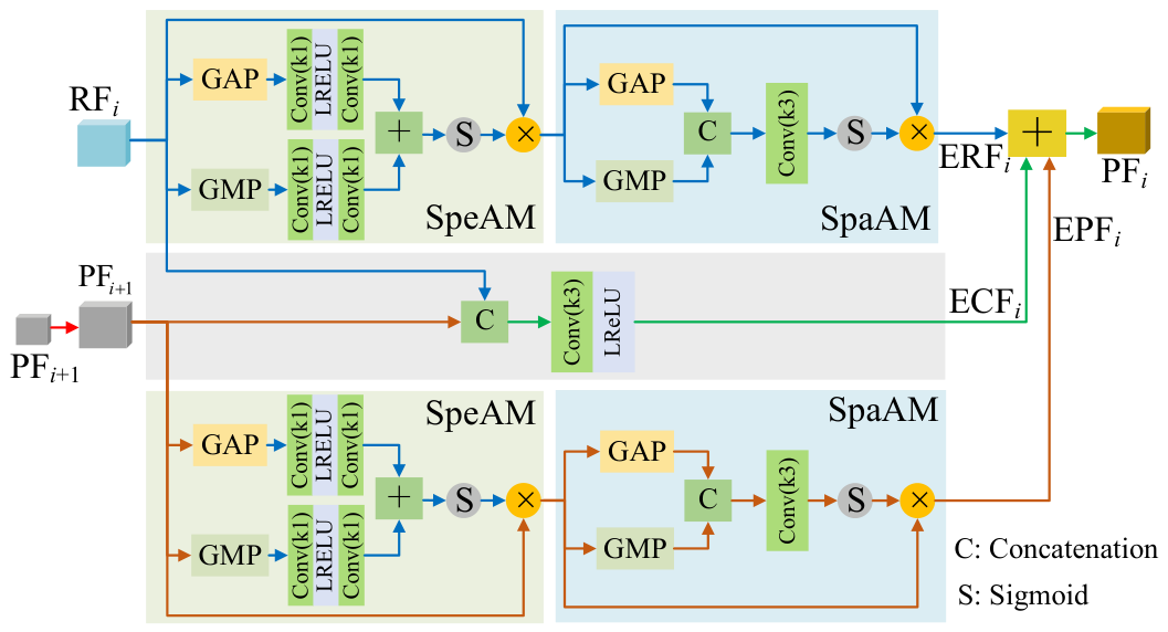
The detailed architecture of DAF is illustrated in Figure 6, which comprises three parallel branches. Specifically, the upper branch adaptively evaluates the importance weights of different spectral channels and spatial positions of the high-spatial resolution cross-fusion feature $\mathrm{R}{\mathrm{F}}_i\left(i=3,2,1\right)$, and performs adaptive attention-weighted enhancement on the critical spectral and spatial information. The lower branch adaptively assesses the importance of spectral channels and spatial locations of the low-spatial resolution decision fusion feature $\mathrm{P}{\mathrm{F}}_{i+1}\left(i=3,2,1\right)$ ($\mathrm{P}{\mathrm{F}}_4=\mathrm{R}{\mathrm{F}}_4$), and dynamically strengthens critical spectral and spatial information. The middle branch is dedicated to integrating the complementary information from both the low-spatial-resolution and the high-spatial-resolution fusion features. Finally, the results of the three branches are added to obtain the refined DAF result $\mathrm{P}{\mathrm{F}}_i\left(i=3,2,1\right)$ at high-spatial resolution. The implementation process is presented in Equations (23) and (24).

$${\mathrm{ERF}}_i=\left[\mathrm{R}{\mathrm{F}}_i·f_{\mathrm{SpeAM}}\left(\mathrm{R}{\mathrm{F}}_i\right)\right]·f_{\mathrm{SpaAM}}\left(\mathrm{R}{\mathrm{F}}_i·f_{\mathrm{SpeAM}}\left(\mathrm{R}{\mathrm{F}}_i\right)\right)\hspace{1em}i=3,2,1$$

(23)

$${\mathrm{EPF}}_i=\left[\widehat{\mathrm{P}{\mathrm{F}}_{i+1}}·f_{\mathrm{SpeAM}}\left(\widehat{\mathrm{P}{\mathrm{F}}_{i+1}}\right)\right]·f_{\mathrm{SpaAM}}\left(\widehat{\mathrm{P}{\mathrm{F}}_{i+1}}·f_{\mathrm{SpeAM}}\left(\widehat{\mathrm{P}{\mathrm{F}}_{i+1}}\right)\right)\hspace{1em}i=3,2,1$$

(24)

$${\mathrm{ECF}}_i=f_{\mathrm{cvl}}^3\left(f_{\mathrm{cat}}\left(\mathrm{R}{\mathrm{F}}_i,\widehat{\mathrm{P}{\mathrm{F}}_{i+1}}\right)\right)\hspace{1em}i=3,2,1$$

(25)

$$\mathrm{P}{\mathrm{F}}_i={\mathrm{ERF}}_i+\mathrm{EP}{\mathrm{F}}_i+\mathrm{EC}{\mathrm{F}}_i\hspace{1em}i=3,2,1$$

(26)

where $f_{\mathrm{SpeAM}}\left( \right)$ denotes the function of the spectral attention module, $f_{\mathrm{SpaAM}}\left( \right)$ represents the function of the spatial attention module, ${\mathrm{ERF}}_i$ is the enhanced feature of $\mathrm{R}{\mathrm{F}}_i$ obtained by spectral-spatial attention adaptive reinforcement, $\widehat{\mathrm{P}{\mathrm{F}}_{i+1}}$ is the upsampled version of ${\mathrm{P}\mathrm{F}}_{i+1}$, ${\mathrm{EPF}}_i$ denotes the enhanced feature of $\mathrm{P}{\mathrm{F}}_i$ obtained by spectral-spatial attention adaptive reinforcement, ${\mathrm{ECF}}_i$ represents the fused feature obtained by integrating the complementary information from $\mathrm{R}{\mathrm{F}}_i$ and ${\mathrm{P}\mathrm{F}}_{i+1}$, and ${\mathrm{P}\mathrm{F}}_i$ denotes the decision fusion feature of DAF.

As illustrated in Figure 6, the upper and lower branches adaptively enhance spectral band information and spatial information of respective importance using a spectral attention module (SpeAM) and a spatial attention module (SpaAM) and adaptively adjust the assignment weights of the fusion results at different stages, thereby achieving more effective feature integration. The implementation process is presented in Equations (27) and (28). Specifically, the SpeAM employs both global average pooling (GAP) and global max pooling (GMP) operations to aggregate the spatial information of each spectral channel, thereby capturing the global contextual characteristics of individual channels. Subsequently, two consecutive convolutions are applied to adaptively learn the complex non-linear interdependencies between different spectral channels. The generated weight coefficients from the two pooling branches are combined via element-wise addition and then processed by a Sigmoid function to produce a spectral channel attention map with values normalized to the range [0, 1]. Finally, this attention map is multiplied element-wise with the original input feature map to achieve channel-wise adaptive feature recalibration.

Correspondingly, the SpaAM applies GAP and GMP operations along the channel dimension to extract the most distinctive structural features (e.g., textures and edges) and overall background characteristics across all channels, and then concatenates them along the channel dimension. Subsequently, a convolution is employed to adaptively fuse and learn the contextual information, followed by a Sigmoid function to generate a spatial attention map with values in [0, 1]. Finally, this spatial attention map is multiplied with each channel feature of the input to adaptively enhance the informative spatial regions.

$$f_{\mathrm{SpeAM}}\left(X\right)=f_{\mathrm{Sigmoid}}\left(f_{\mathrm{cv}}^1\left(f_{\mathrm{cvl}}^1\left(f_{\mathrm{GAP}}\left(X\right)\right)\right)\right.\left.+f_{\mathrm{cv}}^1\left(f_{\mathrm{cvl}}^1\left(f_{\mathrm{GMP}}\left(X\right)\right)\right)\right)$$

(27)

$$f_{\mathrm{SpaAM}}\left(X\right)=f_{\mathrm{Sigmoid}}\left(f_{\mathrm{cv}}^3\left(f_{\mathrm{cat}}\left(f_{\mathrm{GAP}}\left(X\right),f_{\mathrm{GMP}}\left(X\right)\right)\right)\right)$$

(28)

where X denotes the input, $f_{\mathrm{GAP}}\left( \right)$ and $f_{\mathrm{GMP}}\left( \right)$ represent the GAP and GMP operations, and $f_{\mathrm{Sigmoid}}\left( \right)$ refers to the Sigmoid function.

2.3. Convolution-Transformer Discriminator with Multiresolution Inputs

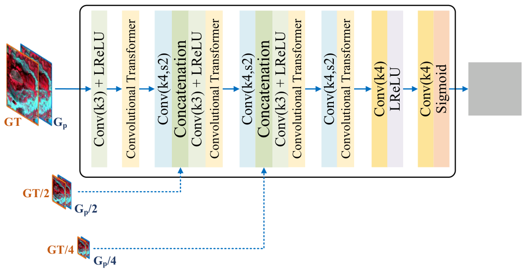
To effectively capture details and temporal variations of ground scenes across diverse scales, an MICTD is designed. The MICTD adversarially learns local and global spectra and details across different resolutions, guiding the TRBG to produce outputs with high perceptual fidelity at all hierarchical resolutions, thereby improving the relative authenticity of the final generated images. As illustrated in Figure 7, the generated multiresolution images ${\mathrm{G}}_{\mathrm{p}}$, ${\displaystyle \frac{{\mathrm{G}}_{\mathrm{p}}}{2}}$, and ${\displaystyle \frac{{\mathrm{G}}_{\mathrm{p}}}{4}}$, together with the ground truth (GT), ${\displaystyle \frac{\mathrm{GT}}{2}}$, and ${\displaystyle \frac{\mathrm{GT}}{4}}$, are fed into the MICTD, enabling the MICTD to perform adversarial learning of hierarchical multiresolution contextual information. Specifically, the high-resolution input branches are dedicated to adversarially learning fine-grained textures, sharp edges, and small-scale ground objects, whereas the low-resolution input branches focus on capturing global scene semantics and spatial relationships.

As depicted in Figure 7, the MICTD first employs a 3 × 3 convolution followed by a convolution-Transformer block to obtain primary local–global features. Subsequently, three consecutive 4 × 4 convolution layers with a stride of 2 are applied to sequentially downsample the feature maps. The downsampled intermediate features are concatenated along the channel dimension with the corresponding 2× and 4× downsampled inputs, then fed into a convolution-Transformer block to produce deep semantic features. Finally, two successive 4 × 4 convolutions with a stride of 1 and a Sigmoid function are used to produce the final authenticity score.

Meanwhile, to accelerate model convergence and significantly enhance training stability and overall performance, spectral normalization [44] is introduced after every convolution. Furthermore, the relative average least squares (RaLS) discriminator [45] is employed to evaluate the relative authenticity of inputs, which further boosts the stability and STF performance.

2.4. Composite Loss Function

To optimize the training stability and fusion capability, a composite loss function is developed, integrating both TRBG and MICTD losses. The TRBG loss comprises not only the RaLS adversarial loss against the MICTD but also the pixel-level reconstruction loss, spectral consistency loss, structural consistency loss, and feature-level perceptual loss.

The adversarial loss for the TRBG and the MICTD is formulated as in Equation (29).

$$\underset{TRBG}{min}\underset{MICTD}{max}\mathcal{L}\left(TRBG,MICTD\right)$$

(29)

The RaLS expressions for the TRBG and MICTD are formulated as Equations (30) and (31).

$${\mathcal{L}}_{TRBG}^{RaLS}={\mathbb{E}}_{T\sim \mathcal{T}}\left[{\left(C\left(T\right)-{\mathbb{E}}_{F\sim \mathcal{F}}\left[C\left(F\right)\right]+1\right)}^2\right]+{\mathbb{E}}_{F\sim \mathcal{F}}\left[{\left(C\left(F\right)-{\mathbb{E}}_{T\sim \mathcal{T}}\left[C\left(T\right)\right]-1\right)}^2\right]$$

(30)

$${\mathcal{L}}_{MICTD}^{RaLS}={\mathbb{E}}_{T\sim \mathcal{T}}\left[{\left(C\left(T\right)-{\mathbb{E}}_{F\sim \mathcal{F}}\left[C\left(F\right)\right]-1\right)}^2\right]+{\mathbb{E}}_{F\sim \mathcal{F}}\left[{\left(C\left(F\right)-{\mathbb{E}}_{T\sim \mathcal{T}}\left[C\left(T\right)\right]+1\right)}^2\right]$$

(31)

where ${\mathcal{L}}_{TRBG}^{RaLS}$ indicates the adversarial loss between the TRBG and MICTD, ${\mathcal{L}}_{MICTD}^{RaLS}$ denotes the MICTD loss, $C\left(·\right)$ refers to the raw logit output of the MICTD, $\mathcal{T}$ signifies the distribution of real images, $\mathcal{F}$ denotes the distribution of generated images, and ${\mathbb{E}}_{T\sim \mathcal{T}}$ and ${\mathbb{E}}_{F\sim \mathcal{F}}$ perform the averaging operation over all reference images and generated images in a batch.

To maintain pixel-level content consistency between the generated image and the real image, the content loss function ${\mathcal{L}}_{MSE}$ is formulated in Equation (32).

$${\mathcal{L}}_{MSE}={\displaystyle \frac{1}{M}}{\displaystyle \sum _{m=1}^M}{\left(GT-G_p\right)}^2$$

(32)

where M denotes the batch size, $GT$ represent the real image, and $G_p$ is the generated image.

To enforce consistency in spatial structure between the generated image and the GT, multiscale structural similarity (MS-SSIM) is adopted to characterize spatial consistency, evaluating the spatial structure similarity from three aspects: luminance l, contrast c, and structure s. The spatial consistency loss function ${\mathcal{L}}_{MS-SSIM}$ is formulated in Equation (33).

$$\begin{array}{c}{\mathcal{L}}_{MS-SSIM}=1-MS\_SSIM\left(GT,G_p\right)\hfill \\ =1-{\left[l_Z\left(GT,G_p\right)\right]}^{{\alpha }_Z}·{\displaystyle \prod _{\tau =1}^Z}{\left[c_{\tau }\left(GT,G_p\right)\right]}^{{\beta }_{\tau }}·{\left[s_{\tau }\left(GT,G_p\right)\right]}^{{\gamma }_{\tau }}\hfill \end{array}$$

(33)

where $MS\_SSIM$ denotes the multiscale structure similarity; $l_Z\left( \right)$, $c_{\tau }\left( \right)$, and $s_{\tau }\left( \right)$ are the luminance at scale Z, contrast at scale $\tau$, and structure at scale $\tau$; ${\alpha }_Z$, ${\beta }_{\tau }$, and ${\gamma }_{\tau }$ are parameters that determine the importance of the l, c, and s components. The mathematical formulations for l, c, and s are presented in Equation (34).

$$\left\{\begin{array}{c}l\left(GT,G_p\right)={\displaystyle \frac{2{\mu }_{GT}{\mu }_{G_p}+{\lambda }_1}{{\mu }_{GT}^2+{\mu }_{G_p}^2+{\lambda }_1}}\hfill \\ c\left(GT,G_p\right)={\displaystyle \frac{2{\sigma }_{GT}{\sigma }_{G_p}+{\lambda }_2}{{\sigma }_{GT}^2+{\sigma }_{G_p}^2+{\lambda }_2}}\hfill \\ s\left(GT,G_p\right)={\displaystyle \frac{{\sigma }_{GT,G_p}+{\lambda }_3}{{\sigma }_{GT}{\sigma }_{G_p}+{\lambda }_3}}\hfill \end{array}\right.$$

(34)

To enforce spectral consistency between the generated images and real images, the spectral angle loss (SAL) is employed to quantitatively evaluate and constrain the spectral distortion. The spectral consistency loss function ${\mathcal{L}}_{spe}$ is formulated in Equation (35).

$${\mathcal{L}}_{spe}=\vartheta \left(GT,G_p\right)=arccos\left({\displaystyle \frac{\overrightarrow{GT}·{\overrightarrow{G_p}}^{\prime }}{\sqrt{{\overrightarrow{GT}}^{\prime }·\overrightarrow{GT}}\sqrt{{\overrightarrow{G_p}}^{\prime }·\overrightarrow{G_p}}}}\right)$$

(35)

where $\overrightarrow{GT}$ and $\overrightarrow{G_p}$ denote the pixel vectors of the GT and generated images, ${\overrightarrow{GT}}^{\prime }$ and ${\overrightarrow{G_p}}^{\prime }$ represent the transposed vectors of the $\overrightarrow{GT}$ and $\overrightarrow{G_p}$, and $\vartheta \left( \right)$ is the spectral angle between the $\overrightarrow{GT}$ and $\overrightarrow{G_p}$ vectors.

To enforce feature-level perceptual consistency between the generated image and the real image, the feature loss ${\mathcal{L}}_{FL}$ is defined as minimizing the distance between the two feature representations before the activation function in the pretrained VGG-19 model [46]. The feature loss is expressed in Equation (36).

$${\mathcal{L}}_{FL}={\displaystyle \frac{1}{M}}{\displaystyle \sum _{m=1}^M}{\left(f_{\mathrm{VGG}}\left(GT\right)-f_{\mathrm{VGG}}\left(G_p\right)\right)}^2$$

(36)

where $f_{\mathrm{VGG}}\left(GT\right)$ and $f_{\mathrm{VGG}}\left(G_p\right)$ denote the feature maps extracted from the pretrained VGG-19 network for the real and generated images only with the red-green-blue band.

Consequently, the total loss function ${\mathcal{L}}_{TL}$ is formulated in Equation (37), where ${\epsilon }_1,{\nu }_2,{\eta }_3,{\gamma }_4$, and ${\zeta }_5$ are the weighting coefficients that control the relative contributions of individual loss terms.

$${\mathcal{L}}_{TL}={\epsilon }_1{\mathcal{L}}_{TRBG}^{RaLS}+{\nu }_2{\mathcal{L}}_{MSE}+{\eta }_3{\mathcal{L}}_{MS-SSIM}+{\gamma }_4{\mathcal{L}}_{spe}+{\zeta }_5{\mathcal{L}}_{FL}$$

(37)

2.5. Training Procedure

In the above elaboration, Algorithm 1 displays the training specifics of the TRB-GAN. First, initialize parameters of the TRBG and MICTD, and define hyperparameters. The GT (Landsat images acquired on the prediction date) is downsampled by the factors of 2 and 4, obtaining 3-scale images, i.e., GT, GT/2, and GT/4. Next, first freeze the TRBG and optimize the MICTD q steps; then fix the MICTD and optimize the TRBG. Last, iterate the preceding procedure until the optimal model is gained.

Algorithm 1 Training specifics of the TRB-GAN

Input:   Fine-resolution and coarse-resolution images at an arbitrary time (F* and C*) and the coarse-resolution image at the prediction time (Cp) Output:   The generated Landsat image at the prediction date (Gp)   1: Initialize parameters of the TRBG and MICTD and define hyperparameters   2: Obtain the downsampled GT images by the factors of 2 and 4: GT/2 and GT/4   3: for k epochs do   4:     Freeze parameters of the TRBG   5:     for q steps do   6:         Select M Gp images with 3-scale produced by the TRBG:   7:         $\left\{{{\mathrm{G}}_{\mathrm{p}}}^{\left(1\right)},\cdots {{\mathrm{G}}_{\mathrm{p}}}^{\left(M\right)}\right\}$, $\left\{{{\displaystyle \frac{{\mathrm{G}}_{\mathrm{p}}}{2}}}^{\left(1\right)},\cdots ,{{\displaystyle \frac{{\mathrm{G}}_{\mathrm{p}}}{2}}}^{\left(M\right)}\right\}$, and $\left\{{{\displaystyle \frac{{\mathrm{G}}_{\mathrm{p}}}{4}}}^{\left(1\right)},\cdots ,{{\displaystyle \frac{{\mathrm{G}}_{\mathrm{p}}}{4}}}^{\left(M\right)}\right\}$   8:         Select M GT images with 3-scale:   9:         $\left\{\mathrm{G}{\mathrm{T}}^{\left(1\right)},\cdots \mathrm{G}{\mathrm{T}}^{\left(M\right)}\right\}$, $\left\{{{\displaystyle \frac{\mathrm{GT}}{2}}}^{\left(1\right)},\cdots ,{{\displaystyle \frac{\mathrm{GT}}{2}}}^{\left(M\right)}\right\}$, and $\left\{{{\displaystyle \frac{\mathrm{GT}}{4}}}^{\left(1\right)},\cdots ,{{\displaystyle \frac{\mathrm{GT}}{4}}}^{\left(M\right)}\right\}$ 10:         Extract local–global features and output authenticity discrimination scores 11:         ${\mathcal{L}}_{MICTD}^{RaLS}$ is estimated by Equation (31) 12:         Update the MICTD by the Adam optimizer 13:     end for 14:     Freeze parameters of the MICTD 15:     Select M F*, C*, and Cp images: 16:     $\left\{{{\mathrm{F}}_{*}}^{\left(1\right)},\dots ,{{\mathrm{F}}_{*}}^{\left(M\right)}\right\}$, $\left\{{\mathrm{C}}_{*}^{\left(1\right)},\dots {,\mathrm{C}}_{*}^{\left(M\right)}\right\}$, and $\left\{{\mathrm{C}}_p^{\left(1\right)},\dots {,\mathrm{C}}_p^{\left(M\right)}\right\}$ 17:     Extract low-level semantic features, high-level multiresolution semantic features, and temporal variation semantic features by Equations (1)–(7) 18:     Execute DGCT and MCDAF to dynamically aggregate spectral, spatial, and time-varying features with Equations (12)–(21) and (23)–(28) 19:     Reconstruct the desired-resolution image and two intermediate-resolution images by the Equation (22) 20:     ${\mathcal{L}}_{TL}$ is estimated by Equation (37) 21:     Update the TRBG by Adam optimizer 22: end for 23: Achieve the optimal model 24: Return the final STF result Gp

3. Experimental Results

3.1. Dataset

To comprehensively validate the STF performance of the proposed TRB-GAN model, extensive experiments are conducted on two wide datasets: the Coleambally Irrigation Area (CIA) and Lower Gwydir Catchment (LGC) [47], both of which contain paired Landsat and MODIS images.

The CIA dataset consists of 17 pairs of cloud-free Landsat-MODIS images, where the Landsat images are derived from Landsat-7 ETM+, and the MODIS images are derived from the MODIS Terra MOD09GA Collection 5 product. The Landsat-MODIS images have dimensions of 1720 × 2040 × 6 (width-height-band). The CIA scenes contain numerous small, irregularly shaped agricultural fields that are spatially dispersed and heterogeneous. The CIA dataset includes scenes with significant seasonal phenological changes and a few land cover type changes.

The LGC dataset consists of 14 pairs of cloud-free Landsat-MODIS images, where the Landsat images are derived from Landsat-5 TM, and the MODIS images are derived from the MODIS Terra MOD09GA Collection 5 product. The Landsat-MODIS images have dimensions of 3200 × 2720 × 6. The LGC dataset contains numerous flood disaster scenes with strong spatial heterogeneity. The LGC dataset includes extensive land cover type changes and seasonal phenological changes.

The Landsat and MODIS images in both CIA and LGC are co-registered to a resolution of 25 m, with a resolution ratio of approximately 20. For the CIA dataset, Landsat–MODIS image pairs are randomly selected as the training set (1st–3rd and 10th–17th groups), while the remaining pairs from the 5th–9th groups are used for testing. The CIA images used for training have a size of 1358 × 2032 × 6. For the LGC dataset, Landsat–MODIS image pairs are randomly selected as the training set (1st–6th and 12th–14th groups), while the remaining pairs from the 8th–11th groups are used for testing. The LGC images used for training have a size of 3184 × 2708 × 6.

3.2. Experimental Setup

The proposed TRB-GAN model is compared with several representative and reproduced STF models, including traditional methods (STARFM [13] and FSDAF [34]) and DL-based models (GAN-STFM [20], MLFF-GAN [48], SwinSTFM [22], ECPW-STFN [27], and STFDiff [32]).

The DL-based comparative methods are retrained on the same training set with identical scene splits to ensure a fair comparison. The training configurations for all learning-based methods, including training epochs, batch size, loss functions, and hyperparameters, are set according to the optimal parameters reported in their respective original publications. The number of input data for comparison methods is also determined following the original works: GAN-STFM and ECPW-STFN take two inputs (as shown in Figure 1c), while STARFM, FSDAF, MLFF-GAN, SwinSTFM, and STFDiff take three inputs (as shown in Figure 1b). For all comparative methods, the patch size was uniformly set to 256 × 256 × C, with a stride of 200.

The inputs to the STARFM, FSDAF, MLFF-GAN, and SwinSTFM models contain three images: the Landsat and MODIS images at time $t_0$ (adjacent to the prediction time $t_p$) and the MODIS image at time $t_p$, predicting the Landsat image at time $t_p$. The inputs to GAN-STFM and ECPW-STFN consist of only two images. GAN-STFM uses the Landsat image at an arbitrary time $t_{*}$ and the MODIS image at time $t_p$, while ECPW-STFN uses the Landsat image at time $t_0$ and the MODIS image at time $t_p$ to predict the Landsat image at $t_p$. The inputs of the proposed TRB-GAN model consist of three images, i.e., the Landsat and MODIS images at an arbitrary time $t_{*}$ and the MODIS image at time $t_p$, to predict the Landsat image at time $t_p$.

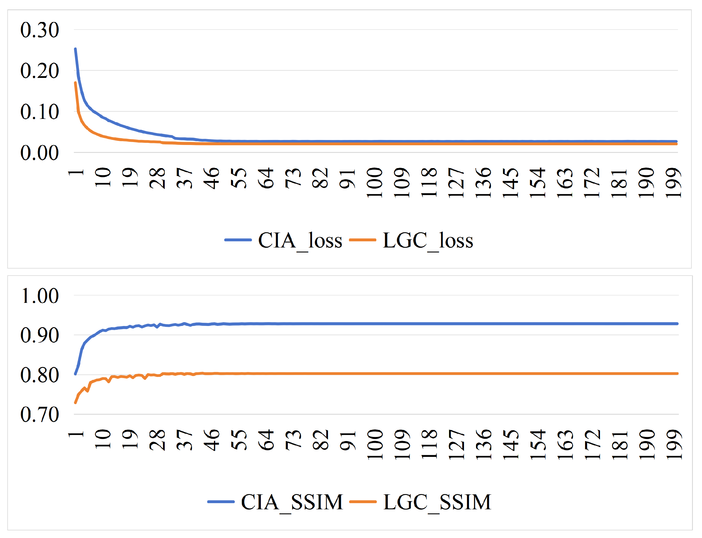
The DL-based models are realized via the PyTorch framework, and the STARFM and FSDAF methods are implemented in IDL. The experimental platform includes two NVIDIA GeForce RTX 4090 GPUs and an AMD Ryzen 9 7950X 16-core processor. The proposed TRB-GAN employs a batch size of 8 and a maximum of 200 epochs. The actual number of epochs can be determined adaptively during training based on the dataset size and the batch size. The number of input and output channels can be configured according to the data. The optimal hyperparameters in the loss function are set to ${\epsilon }_1=1\times {10}^{-3}$ and ${\nu }_2={\eta }_3={\gamma }_4={\zeta }_5=1$. The tuning procedure of hyperparameters is detailed in Appendix B. The Adam optimizer [49] is employed to optimize the model, with an initial learning rate of $2\times {10}^{-4}$. The training loss and SSIM curves on the CIA and LGC datasets are shown in Figure A1. The DL-based models are implemented on GPUs, and traditional models are executed on CPUs.

Both subjective and objective assessments of the STF results are conducted. Quantitative evaluation metrics commonly employed include root mean square error (RMSE), spectral angle mapper (SAM) [50], structural similarity (SSIM) [51], erreur relative globale adimensionnelle de synthèse (ERGAS), and correlation coefficient (CC) [52]. RMSE quantifies the pixel-wise deviation between the ${\mathrm{G}}_{\mathrm{p}}$ and GT images; the closer ${\mathrm{G}}_{\mathrm{p}}$ is to GT, the smaller the RMSE value. SAM calculates the spectral similarity between the spectral vectors of ${\mathrm{G}}_{\mathrm{p}}$ and GT images; the smaller the angle, the more similar the spectra. ERGAS is a global metric for assessing the quality of multispectral images; a lower ERGAS value indicates a smaller overall error between ${\mathrm{G}}_{\mathrm{p}}$ and GT. SSIM measures the perceptual similarity between ${\mathrm{G}}_{\mathrm{p}}$ and GT; the closer is to GT, the closer the SSIM value is to 1. CC measures the degree of linear correlation between ${\mathrm{G}}_{\mathrm{p}}$ and GT; the more positively correlated ${\mathrm{G}}_{\mathrm{p}}$ and GT are, the closer the CC value is to 1. The optimal values for RMSE, SAM, and ERGAS are 0, and the optimal values for SSIM and CC are 1.

3.3. Ablation Experiment

To validate the contributions of core components of the proposed model to the STF performance, i.e., the arbitrary temporal variation information, the bidirectional encoder, the dual-guided cross-convolution attention, the decision attention fusion, and the multiresolution inputs of the MICTD, ablation experiments are conducted. In the tables, bold values indicate the best results and underlined values indicate the second-best results among the compared models.

3.3.1. Influence of Prior Time-Varying Information

To verify the influence of different prior data on the predictions for the same scene, prior data from different dates are utilized to predict the CIA scene from 5 January 2002, and the LGC scene from 28 December 2004.

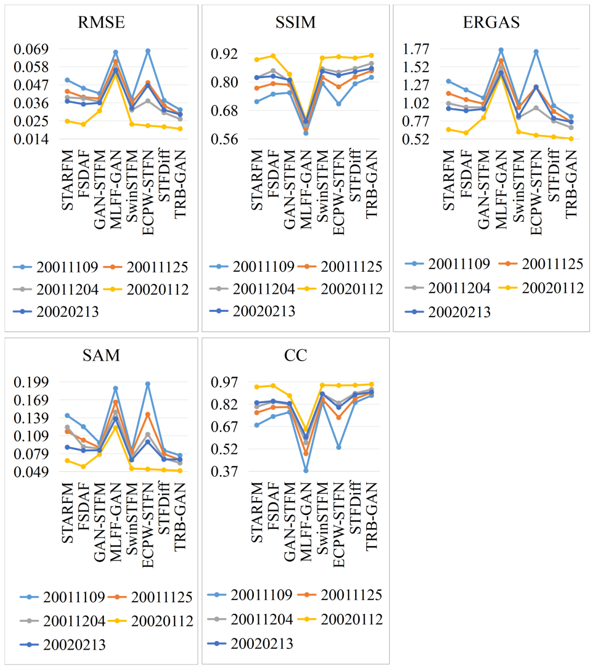
The CIA scene data from 5 January 2002 is predicted utilizing the prior data from 9 November 2001, 25 November 2001, 4 December 2001, 12 January 2002, and 13 February 2002, with dimensions of 2000 × 1200 × 6. The quantitative evaluations of the predictions are displayed in Figure 8. The horizontal axis denotes the compared methods: STARFM, FSDAF, GAN-STFM, MLFF-GAN, SwinSTFM, ECPW-STFN, STFDiff, and the proposed TRB-GAN. On the vertical axis, circles of different colors represent the objective metrics of the CIA predictions of 5 January 2002, obtained by each method using five prior data. From Figure 8, it is evident that comparative methods exhibit distinct prediction performances when using different prior data. Moreover, the metrics of STARFM, MLFF-GAN, SwinSTFM, FSDAF, and ECPW-STFN are considerably affected by the prior data, yet the GAN-STFM, STFDiff, and proposed TRB-GAN are less sensitive across different prior data. Furthermore, TRB-GAN exhibits relatively low sensitivity to varying time intervals in terms of RMSE, SSIM, ERGAS, SAM, and CC metrics. Notably, the proposed TRB-GAN achieves superior metrics under five different prior data.

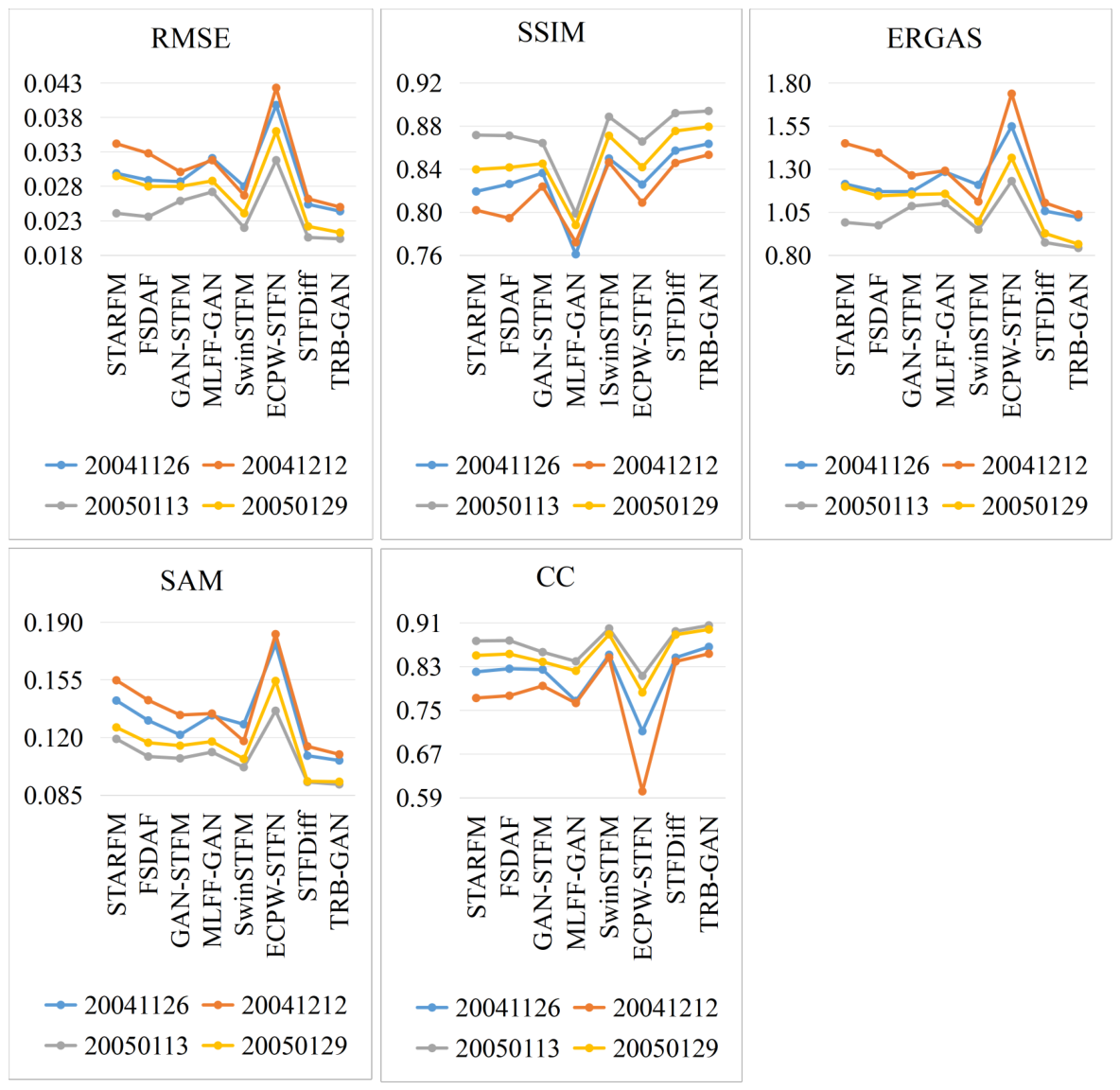
The LGC scene data from 28 December 2004 is predicted utilizing the prior data from 26 November 2004, 12 December 2004, 13 January 2005, and 29 January 2005, with dimensions of 2500 × 3000 × 6. The quantitative evaluations of the predictions are displayed in Figure 9. On the vertical axis, circles of different colors represent the objective metrics of the LGC predictions of 28 December 2004, obtained by each method using four prior data. As clearly illustrated in Figure 9, comparative methods exhibit distinct prediction performances when utilizing different prior data. The STARFM, MLFF-GAN, SwinSTFM, FSDAF, ECPW-STFN, and STFDiff demonstrate substantial variations in quantitative metrics across four prior data. The GAN-STFM and the proposed TRB-GAN exhibit significantly lower sensitivity to the four prior data, with TRB-GAN showing even smaller variation. Moreover, the proposed TRB-GAN achieves superior quantitative performance across four prior data.

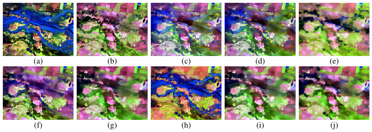
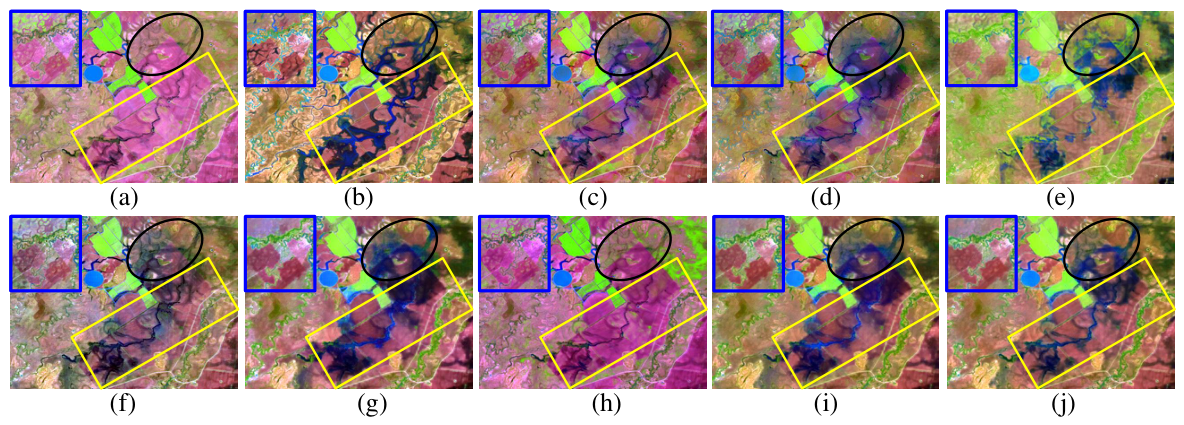
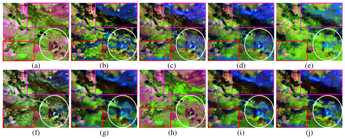
To validate the prediction performance of the proposed TRB-GAN in flood-affected change regions,

Table 1. Objective metric evaluation of the fusion results for the flood-affected region in the LGC scene on 28 December 2004, using prior data from different temporal phases.

Prediction Data	Model	RMSE	CC	SSIM	ERGAS	SAM
20041126 ↓ 20041228	STARFM	0.0304	0.7824	0.8089	1.3294	0.1440
	FSDAF	0.0302	0.7852	0.8135	1.3158	0.1347
	GAN-STFM	0.0333	0.7323	0.8040	1.4847	0.1476
	MLFF-GAN	0.0343	0.7231	0.7439	1.5041	0.1446
	SwinSTFM	0.0309	0.8178	0.8221	1.4734	0.1596
	ECPW-STFN	0.0418	0.7023	0.8016	1.8087	0.1996
	STFDiff	0.0272	0.8110	0.8382	1.2384	0.1286
	TRB-GAN	0.0241	0.8582	0.8543	1.0691	0.1124
20041212 ↓ 20041228	STARFM	0.0425	0.5941	0.7212	2.1582	0.2100
	FSDAF	0.0372	0.6457	0.7395	1.8697	0.1861
	GAN-STFM	0.0335	0.7269	0.7791	1.4796	0.1984
	MLFF-GAN	0.0350	0.6578	0.7440	1.6138	0.1649
	SwinSTFM	0.0302	0.7718	0.8139	1.3852	0.1312
	ECPW-STFN	0.0483	0.4054	0.7555	2.2954	0.3014
	STFDiff	0.0291	0.7757	0.8154	1.3460	0.1319
	TRB-GAN	0.0268	0.8197	0.8307	1.1933	0.1272
20050113 ↓ 20041228	STARFM	0.0247	0.8641	0.8559	1.1056	0.1369
	FSDAF	0.0238	0.8685	0.8639	1.0721	0.1184
	GAN-STFM	0.0293	0.7893	0.8358	1.3629	0.1327
	MLFF-GAN	0.0284	0.8098	0.7809	1.2624	0.1174
	SwinSTFM	0.0235	0.8815	0.8730	1.0905	0.1177
	ECPW-STFN	0.0307	0.8213	0.8514	1.2881	0.1430
	STFDiff	0.0215	0.8750	0.8809	0.9766	0.1012
	TRB-GAN	0.0208	0.8961	0.8862	0.9202	0.0983
20050129 ↓ 20041228	STARFM	0.0402	0.7372	0.8027	1.8882	0.1541
	FSDAF	0.0384	0.7315	0.8123	1.8238	0.1361
	GAN-STFM	0.0309	0.7639	0.8178	1.4187	0.1342
	MLFF-GAN	0.0313	0.7628	0.7634	1.3908	0.1267
	SwinSTFM	0.0284	0.8245	0.8497	1.2831	0.1226
	ECPW-STFN	0.0360	0.7562	0.8232	1.5182	0.1565
	STFDiff	0.0255	0.8362	0.8592	1.1591	0.1069
	TRB-GAN	0.0226	0.8724	0.8688	1.0016	0.1014

presents the evaluation metrics of the fusion results over flood areas generated by different comparative methods using multitemporal data. Figure 10 provides a visual comparison of the prediction results for 28 December 2004, using the prior data from 12 December 2004. From Table 1, it is evident that the proposed TRB-GAN achieves superior performance across RMSE, CC, SSIM, ERGAS, and SAM metrics for the prediction results in the flood region on 28 December 2004, using prior data from 26 November 2004, 12 December 2004, 13 January 2005, and 29 January 2005. Figure 10a presents the Landsat image acquired on 12 December 2004; Figure 10b shows the reference Landsat image acquired on 28 December 2004 (GT). Figure 10c–j display the prediction results of STARFM, FSDAF, GAN-STFM, MLFF-GAN, SwinSTFM, ECPW-STFN, STFDiff, and TRB-GAN. From Figure 10, it can be clearly observed that STARFM, FSDAF, MLFF-GAN, and ECPW-STFN yield poor predictive performance in the flood-affected areas. GAN-STFM suffers from more pronounced spectral and spatial distortions. Compared with SwinSTFM and STFDiff, the proposed TRB-GAN produces prediction results that are more closely aligned with the GT.

The above results demonstrate that the proposed TRB-GAN exhibits minimal sensitivity to the prior data when predicting numerous scenes with seasonal phenological variations and land cover type transitions and consistently achieves superior STF performance. This further verifies that the proposed TRB-GAN model possesses excellent stability and strong robustness in handling predictions for different types of changes and across varying temporal intervals for the CIA and LGC data.

3.3.2. Effectiveness of the Bidirectional Encoder

To validate the effectiveness of bidirectional encoding of temporal variation information and prior information, the temporal variation information encoding branch is modified to extract multiscale temporal variation features in the high-to-low resolution manner, the same as the prior information encoding branch. All other components of the proposed model remain unchanged, denoted as DFE. The objective metrics of the fusion results on the CIA and LGC test data are presented in

Table 2. Quantitative evaluation of ablation experiment results for the DFE, w/o DAF, and TDAF models on three test data of CIA.

Prediction Data	Model	RMSE	CC	SSIM	ERGAS	SAM
20011125 ↓ 20011204	DFE	0.0270	0.8911	0.8724	0.7730	0.0788
	w/o DAF	0.0263	0.8936	0.8758	0.7444	0.0797
	TDAF	0.0226	0.9198	0.8837	0.6422	0.0665
	TRB-GAN	0.0215	0.9269	0.8970	0.6062	0.0571
20011204 ↓ 20020105	DFE	0.0331	0.8666	0.8456	0.8499	0.0796
	w/o DAF	0.0319	0.8736	0.8512	0.8202	0.0784
	TDAF	0.0266	0.9123	0.8615	0.6910	0.0640
	TRB-GAN	0.0261	0.9193	0.8780	0.6791	0.0635
20020112 ↓ 20020213	DFE	0.0250	0.9151	0.8748	0.8104	0.0706
	w/o DAF	0.0251	0.9115	0.8716	0.8194	0.0738
	TDAF	0.0238	0.9214	0.8730	0.7704	0.0695
	TRB-GAN	0.0227	0.9234	0.8817	0.7435	0.0656

and

Table 3. Quantitative evaluation of ablation experiment results for the DFE, w/o DAF, and TDAF models on two test data of LGC.

Prediction Data	Model	RMSE	CC	SSIM	ERGAS	SAM
20041126 ↓ 20041212	DFE	0.0318	0.7797	0.7995	1.6611	0.1778
	w/o DAF	0.0315	0.7766	0.8040	1.6411	0.1712
	TDAF	0.0310	0.7806	0.7994	1.5975	0.1901
	TRB-GAN	0.0291	0.7995	0.8087	1.5053	0.1690
20041228 ↓ 20050113	DFE	0.0183	0.9229	0.9167	0.6344	0.0602
	w/o DAF	0.0171	0.9255	0.9200	0.5816	0.0595
	TDAF	0.0177	0.9217	0.9164	0.6061	0.0636
	TRB-GAN	0.0158	0.9312	0.9213	0.5441	0.0583

. 20011125⟶20011204 indicates that the prior data is from 25 November 2001, and the forecast is for 4 December 2001. As clearly observed in Table 2 and Table 3, on the three CIA and two LGC test data, the fusion results of DFE are inferior to those of the proposed TRB-GAN in RMSE, SAM, CC, SSIM, and ERGAS. This demonstrates the effectiveness of the temporal variation information encoding branch in extracting multiscale features from low-to-high resolution via super-resolution, which confirms that the bidirectional encoder enhances STF capability and information fidelity.

3.3.3. Effectiveness of Decision Attention Fusion

The DAF is a crucial component of the DTAFD. To demonstrate the effectiveness of DAF, the following ablation experiments are conducted. (1) Fusion is performed using concatenation+convolution+LReLU, removing the attention branches in DAF, denoted as w/o DAF. (2) The middle concatenation fusion branch of DAF is removed, retaining the attention branches, denoted as TDAF. Table 2 and Table 3 present the metrics of the fusion results on the CIA and LGC test dataset for the variants w/o DAF and TDAF. As clearly observed from Table 2 and Table 3, the fusion performance of w/o DAF and TDAF in RMSE, SAM, CC, SSIM, and ERGAS degrades compared with that of the TRB-GAN. This demonstrates the positive role of DAF in aggregating and restoring spectra and details, effectively improving the STF capability.

3.3.4. Effectiveness of Dual-Guided Cross Convolution-Transformer

DGCT is a crucial module in the DTAFD. To prove the role of DGCT, the following ablation experiments are performed. (1) Replace DGCT with cross convolution-Transformer fusion guided by prior feature $\mathrm{F}{\mathrm{F}}_i$, i.e., retain the right branch of DGCT, denoted as PFD; (2) Replace DGCT with cross convolution-Transformer fusion guided by time-varying feature $\mathrm{C}{\mathrm{F}}_{4-i+1}$, i.e., retain the left branch of DGCT, denoted as CFD. The metrics of the fusion results of PFD and CFD on the CIA and LGC test data are shown in

Table 4. Quantitative evaluation of ablation experiment results for the PFD and CFD models on three test data of CIA.

Prediction Data	Model	RMSE	CC	SSIM	ERGAS	SAM
20011125 ↓ 20011204	PFD	0.0278	0.8866	0.8721	0.7998	0.0807
	CFD	0.0240	0.9153	0.8801	0.6895	0.0677
	TRB-GAN	0.0215	0.9269	0.8970	0.6062	0.0571
20011204 ↓ 20020105	PFD	0.0312	0.8817	0.8527	0.8051	0.0742
	CFD	0.0277	0.9104	0.8558	0.7595	0.0695
	TRB-GAN	0.0261	0.9193	0.8780	0.6791	0.0635
20020112 ↓ 20020213	PFD	0.0242	0.9164	0.8767	0.7834	0.0678
	CFD	0.0252	0.9193	0.8699	0.8308	0.0704
	TRB-GAN	0.0227	0.9234	0.8817	0.7435	0.0656

and

Table 5. Quantitative evaluation of ablation experiment results for the PFD and CFD models on two test data of LGC.

Prediction Data	Model	RMSE	CC	SSIM	ERGAS	SAM
20041126 ↓ 20041212	PFD	0.0327	0.7783	0.8007	1.7205	0.1787
	CFD	0.0317	0.7751	0.8034	1.6461	0.1730
	TRB-GAN	0.0291	0.7995	0.8087	1.5053	0.1690
20041228 ↓ 20050113	PFD	0.0175	0.9196	0.9184	0.6089	0.0605
	CFD	0.0168	0.9279	0.9209	0.5706	0.0590
	TRB-GAN	0.0158	0.9312	0.9213	0.5441	0.0583

. As clearly illustrated in Table 4 and Table 5, the CFD achieves better prediction metrics than the PFD on the CIA scenes of 4 December 2001, and 5 January 2002, and the two LGC scenes, whereas the PFD outperforms the CFD on the CIA scene of 13 February 2002. In the three CIA and two LGC scenes, both PFD and CFD exhibit degraded fusion performance in RMSE, SAM, CC, SSIM, and ERGAS compared to the TRB-GAN. This demonstrates the positive roles of PFD and CFD in effectively aggregating prior and temporal variation information, thereby effectively improving STF capability.

3.3.5. Validity of Multiresolution Input for MICTD

To verify the impact of multiresolution inputs from the MICTD on the STF capability, adversarial training is performed using fusion results at distinct resolutions paired with the GT as inputs, as demonstrated in the following ablation experiments: (1) Adversarial training with ${\mathrm{G}}_{\mathrm{p}}$ and GT as inputs to the MICTD, denoted as ORI; (2) Adversarial training with (${\mathrm{G}}_{\mathrm{p}}$, GT) and (${\displaystyle \frac{{\mathrm{G}}_{\mathrm{p}}}{2}}$, ${\displaystyle \frac{\mathrm{GT}}{2}}$) as inputs to the MICTD, denoted as TRI. The objective evaluation of the fusion results on the CIA and LGC test data is presented in

Table 6. Quantitative evaluation of ablation experiment results for the ORI and TRI models on three test data of CIA.

Prediction Data	Model	RMSE	CC	SSIM	ERGAS	SAM
20011125 ↓ 20011204	ORI	0.0281	0.8857	0.8700	0.8129	0.0826
	TRI	0.0226	0.9205	0.8825	0.6367	0.0657
	TRB-GAN	0.0215	0.9269	0.8970	0.6062	0.0571
20011204 ↓ 20020105	ORI	0.0311	0.8862	0.8546	0.7988	0.0726
	TRI	0.0265	0.9132	0.8597	0.6890	0.0650
	TRB-GAN	0.0261	0.9193	0.8780	0.6791	0.0635
20020112 ↓ 20020213	ORI	0.0240	0.9187	0.8771	0.7731	0.0673
	TRI	0.0247	0.9206	0.8709	0.7920	0.0733
	TRB-GAN	0.0227	0.9234	0.8817	0.7435	0.0656

and

Table 7. Quantitative evaluation of ablation experiment results for the ORI and TRI models on two test data of LGC.

Prediction Data	Model	RMSE	CC	SSIM	ERGAS	SAM
20041126 ↓ 20041212	ORI	0.0328	0.7781	0.7921	1.7074	0.1784
	TRI	0.0312	0.7780	0.8006	1.6215	0.1757
	TRB-GAN	0.0291	0.7995	0.8087	1.5053	0.1690
20041228 ↓ 20050113	ORI	0.0180	0.9157	0.9151	0.6221	0.0632
	TRI	0.0175	0.9214	0.9175	0.6046	0.0630
	TRB-GAN	0.0158	0.9312	0.9213	0.5441	0.0583

. As clearly illustrated in Table 6 and Table 7, the TRI achieves better prediction metrics than ORI on the CIA scenes of 4 December 2001, and 5 January 2002, and the LGC scenes of 12 December 2004, and 13 January 2005, whereas the ORI outperforms TRI in RMSE, SSIM, ERGAS, and SAM on the CIA scene of 13 February 2002. Therefore, four repeated experiments with different seeds for ORI, TRI, and TRB-GAN are conducted; the mean and standard deviation of five core metrics are calculated. On the CIA scene of 13 February 2002, the TRI achieves consistently lower mean ERGAS (0.7824 ± 0.0103 vs. 0.7871 ± 0.0137) and SAM (0.0720 ± 0.001 vs. 0.0730 ± 0.0049) and higher mean SSIM (0.8762 ± 0.0041 vs. 0.8755 ± 0.0025) and CC (0.9194 ± 0.0021 vs. 0.9164±0.0035) than ORI, while the differences in RMSE (0.0242 ± 0.0004 vs. 0.0242 ± 0.0002) are negligible. From the perspective of average performance over four repeated trials, TRI brings neutral-to-positive fusion gains and does not induce universal performance degradation. In addition, the TRB-GAN outperforms both ORI and TRI on five metrics with the smallest standard deviation, fully verifying the complementary benefits of multiresolution components. These findings also indicate that the ORI and TRI may exhibit varying performance under distinct scenarios. However, on the three CIA and two LGC scenes, the fusion results of ORI and TRI both exhibit inferior performance compared to the proposed TRB-GAN across the RMSE, SAM, CC, SSIM, and ERGAS metrics. This verifies the positive role of adversarial learning on multiresolution data for the proposed model, enhancing both the STF capability and fidelity.

3.4. Comparative Experiment and Analysis

3.4.1. Experiments on the CIA Dataset

Table 8. Objective metrics of comparative fusion results on the CIA dataset.

Prediction Data	Model	RMSE	ERGAS	SAM	CC	SSIM
20011109 ↓ 20011125	STARFM	0.0303	1.0356	0.1079	0.8088	0.8304
	FSDAF	0.0299	1.0230	0.1121	0.8105	0.8310
	GAN-STFM	0.0322	1.0777	0.1236	0.7964	0.8134
	MLFF-GAN	0.0465	1.5002	0.1379	0.6118	0.6793
	SwinSTFM	0.0269	0.8839	0.0953	0.8659	0.8541
	ECPW-STFN	0.0286	0.9967	0.1081	0.8557	0.8517
	STFDiff	0.0267	0.8984	0.0946	0.8614	0.8507
	TRB-GAN	0.0234	0.7849	0.0760	0.8934	0.8682
20011125 ↓ 20011204	STARFM	0.0301	0.8925	0.0890	0.8612	0.8672
	FSDAF	0.0300	0.9057	0.0884	0.8785	0.8715
	GAN-STFM	0.0326	0.9388	0.1014	0.8161	0.8342
	MLFF-GAN	0.0501	1.3847	0.1260	0.6159	0.6678
	SwinSTFM	0.0286	0.8504	0.0831	0.8912	0.8699
	ECPW-STFN	0.0292	0.8460	0.0851	0.8758	0.8710
	STFDiff	0.0268	0.7618	0.0781	0.8919	0.8731
	TRB-GAN	0.0215	0.6062	0.0571	0.9269	0.8970
20011204 ↓ 20020105	STARFM	0.0393	1.0126	0.1235	0.8038	0.8185
	FSDAF	0.0387	0.9601	0.0907	0.8368	0.8476
	GAN-STFM	0.0367	0.9581	0.0876	0.8182	0.8040
	MLFF-GAN	0.0578	1.5127	0.1487	0.5618	0.6176
	SwinSTFM	0.0316	0.8166	0.0729	0.8900	0.8556
	ECPW-STFN	0.0372	0.9520	0.1114	0.8278	0.8411
	STFDiff	0.0300	0.7690	0.0715	0.8935	0.8569
	TRB-GAN	0.0261	0.6791	0.0635	0.9193	0.8780
20020105 ↓ 20020112	STARFM	0.0290	0.9248	0.0842	0.9383	0.8785
	FSDAF	0.0239	0.8311	0.0714	0.9347	0.8920
	GAN-STFM	0.0287	0.8477	0.0794	0.8916	0.8493
	MLFF-GAN	0.0517	1.4905	0.1297	0.6446	0.6348
	SwinSTFM	0.0206	0.5965	0.0547	0.9476	0.9103
	ECPW-STFN	0.0223	0.6806	0.0578	0.9565	0.9175
	STFDiff	0.0199	0.5887	0.0533	0.9496	0.9114
	TRB-GAN	0.0196	0.5861	0.0491	0.9554	0.9176
20020112 ↓ 20020213	STARFM	0.0330	1.0989	0.1045	0.8491	0.8122
	FSDAF	0.0328	1.1656	0.1157	0.8569	0.8308
	GAN-STFM	0.0261	0.8593	0.0802	0.8963	0.8555
	MLFF-GAN	0.0481	1.5952	0.1568	0.6648	0.6517
	SwinSTFM	0.0241	0.8237	0.0727	0.9162	0.8755
	ECPW-STFN	0.0339	1.1664	0.0971	0.8656	0.8461
	STFDiff	0.0242	0.7783	0.0696	0.9179	0.8755
	TRB-GAN	0.0227	0.7435	0.0656	0.9234	0.8817

presents the objective evaluation of the STF results obtained by the compared methods and the proposed TRB-GAN model on the five groups of test data from CIA, with dimensions of 2000 × 1200 × 6.

As clearly observed in Table 8, the proposed TRB-GAN model achieves superior performance in RMSE, ERGAS, SAM, CC, and SSIM metrics across the first, second, third, and fifth groups of CIA test data. In the fourth group of CIA test data, the proposed TRB-GAN model achieves optimal performance in RMSE, ERGAS, SAM, and SSIM metrics and ranks second on the CC metric, differing from the optimal result by only 0.0011. Although the majority of indicators for STFDiff rank second-best, there are still cases where the RMSE, ERGAS, and CC metrics fall below the suboptimal level. The SwinSTFM performs slightly worse than the STFDiff on most metrics. The FSDAF outperforms GAN-STFM on the first, second, and fourth test data, whereas the GAN-STFM yields better results than FSDAF on the fifth test data. The ECPW-STFN ranks third in the metrics of the fusion results on the first, second, and fourth test data, while the metrics for the fusion results on the third and fifth test data are relatively poor.

The above proves that the fusion results of the proposed TRB-GAN model achieve superior spectral and detail fidelity, yield more favorable prediction results in scenarios with significant phenological variations, and demonstrate more robust STF stability and robustness in the various CIA scenarios.

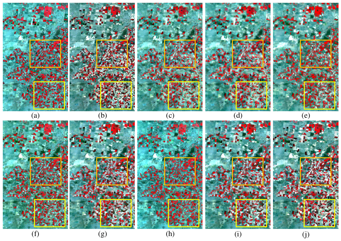
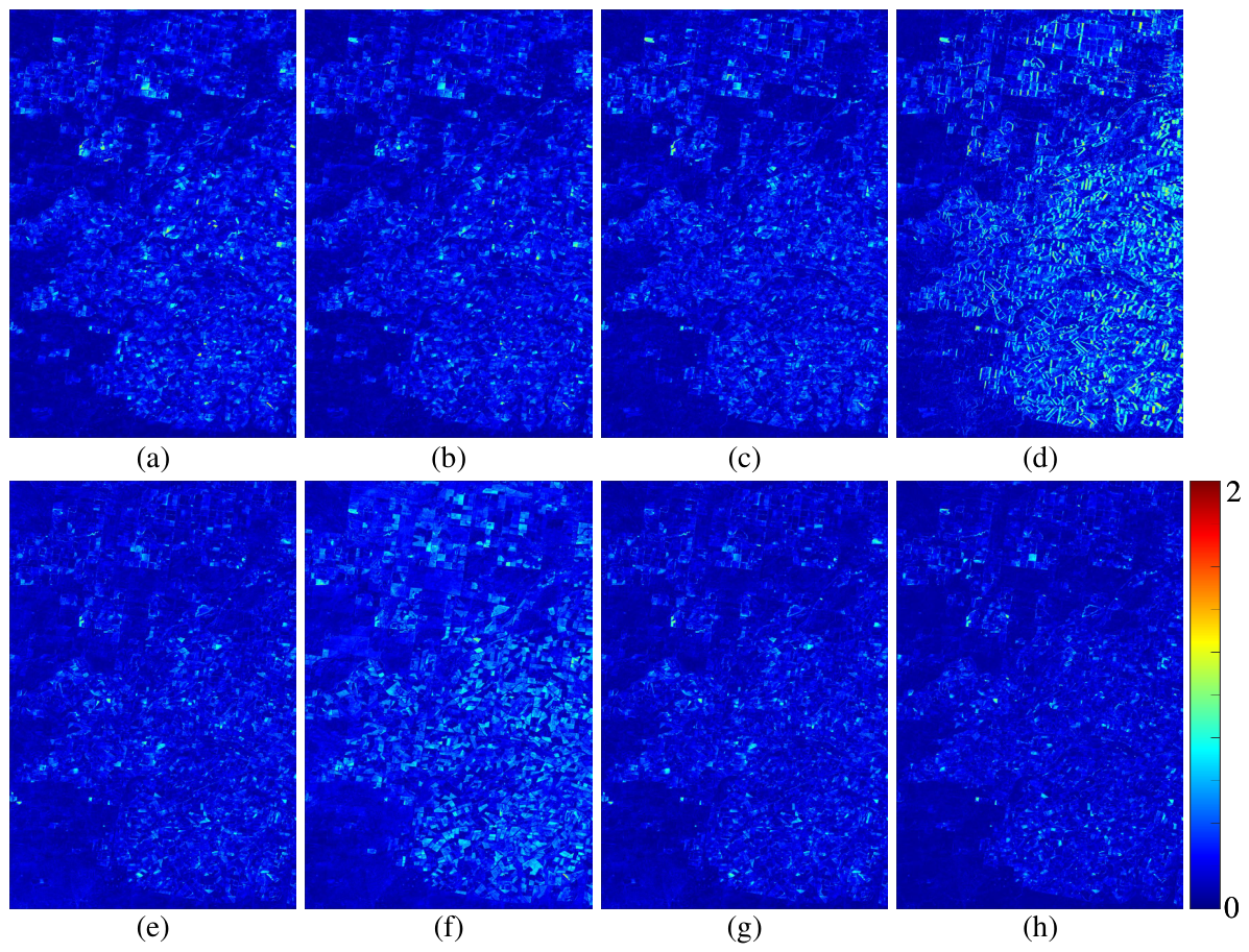
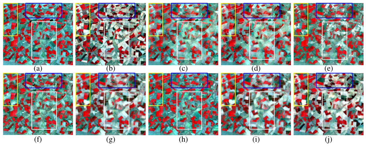
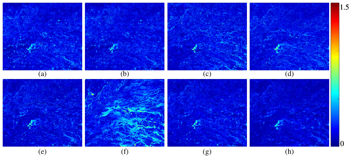
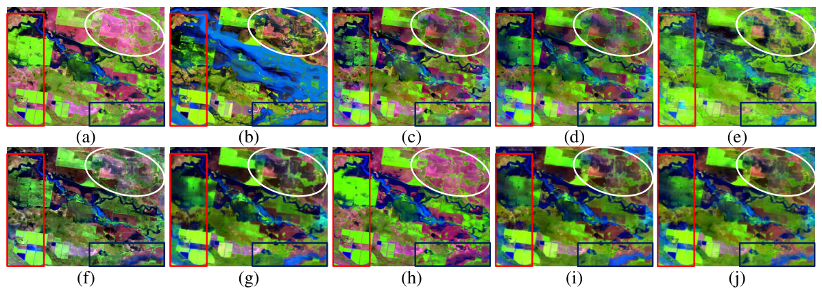
For visual evaluation, the CIA scene exhibits extensive phenological changes. Figure 11 illustrates the prediction results for the CIA scene of 5 January 2002, using the prior data from 13 February 2002, with the near-infrared, red, and green bands assigned to the R, G, and B channels. The Landsat and MODIS images from 13 February 2002, serve as the prior data (GAN-STFM only uses the Landsat image), and the Landsat scene of 5 January 2002, is the GT. Figure 11a depicts the Landsat image acquired on 13 February 2002, serving as the prior data. Figure 11b displays the Landsat image obtained on the same date, i.e., the GT. Figure 11c–j present the prediction results for the image in Figure 11b generated by the STARFM, FSDAF, GAN-STFM, MLFF-GAN, SwinSTFM, ECPW-STFN, STFDiff, and the proposed TRB-GAN method. The mean absolute error maps (MAEMs) between the predicted results and the GT are illustrated in Figure 12.

Figure 11 clearly demonstrates that the fusion results generated by STARFM, FSDAF, GAN-STFM, MLFF-GAN, and ECPW-STFN exhibit spectral characteristics closer to that of the prior data in Figure 11a, achieving relatively low prediction accuracy for land cover changes in the scene and deviating significantly from the GT in spectra. In contrast, SwinSTFM, STFDiff, and the proposed TRB-GAN produce predictions for the changed regions that are more consistent with the GT. In Figure 12, the darker the error color, the smaller the discrepancy between the fusion result and the GT; conversely, the brighter the color, the larger the error. As clearly evident from Figure 12, the TRB-GAN result exhibits smaller errors compared to the GT.

The objective evaluation of the prediction results for the CIA scene of 5 January 2002, obtained by the compared methods via the prior data from 13 February 2002, is presented in

Table 9. Quantitative evaluation for predicted results of CIA scene on 5 January 2002, using the prior data of 13 February 2002.

Prediction Data	Model	RMSE	ERGAS	SAM	CC	SSIM
20020213 ↓ 20020105	STARFM	0.0370	0.9418	0.0899	0.8304	0.8185
	FSDAF	0.0352	0.9126	0.0845	0.8411	0.8244
	GAN-STFM	0.0360	0.9353	0.0849	0.8255	0.8081
	MLFF-GAN	0.0559	1.4363	0.1374	0.5991	0.6341
	SwinSTFM	0.0328	0.8383	0.0687	0.8897	0.8450
	ECPW-STFN	0.0466	1.2385	0.0989	0.7988	0.8272
	STFDiff	0.0317	0.8081	0.0696	0.8845	0.8428
	TRB-GAN	0.0289	0.7565	0.0695	0.9018	0.8571

. As clearly observed from Table 9, the proposed TRB-GAN method achieves the best performance in RMSE, ERGAS, CC, and SSIM, although it ranks second best in SAM with a difference of only 0.0008 from the optimal value.

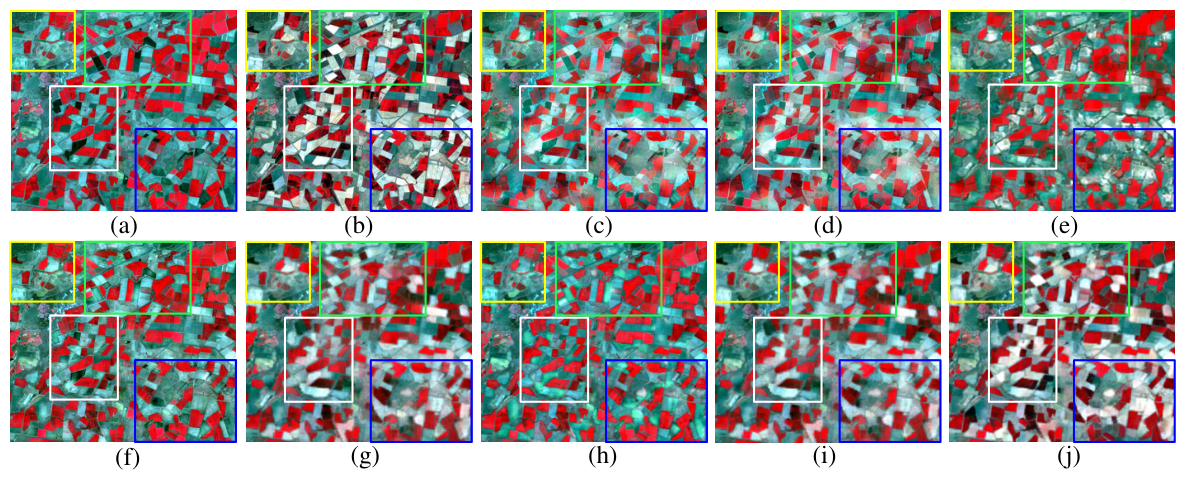
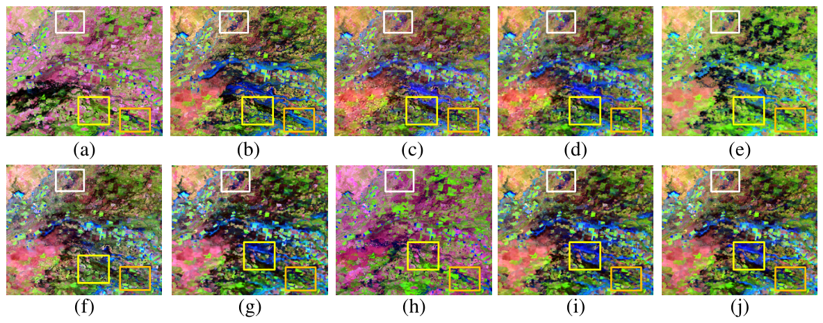
To more clearly compare the prediction performance of various methods for changed scenarios, the areas marked by orange and yellow boxes in Figure 11 are magnified and displayed in Figure 13 and Figure 14. From Figure 13, it is evident that the fused results of the STARFM, GAN-STFM, MLFF-GAN, and ECPW-STFN exhibit significant distortion, are greatly influenced by the prior data in Figure 13a, and demonstrate poor prediction accuracy for changed scenarios. The FSDAF, SwinSTFM, STFDiff, and TRB-GAN methods yield promising predictions for changed regions, as illustrated in the yellow, green, and blue marked areas in Figure 13. By comparison, the spectra and details of the TRB-GAN results are closer to the GT. As observed from Figure 14, the fusion results of STARFM, GAN-STFM, MLFF-GAN, and ECPW-STFN rely on the prior data in Figure 14a, yielding poor prediction performance in changed regions and exhibiting large deviations from the GT. FSDAF exhibits severe distortion in the predictions within the white, blue, and yellow boxes. Compared to SwinSTFM and STFDiff, the TRB-GAN achieves prediction results in changed regions closer to the GT and exhibits fewer spectrum and detail distortions.

In summary, the proposed TRB-GAN method achieves superior STF results in both visual assessment and objective metrics for the CIA dataset, which contains substantial phenological variations, and demonstrates higher STF stability and robustness over large temporal intervals for the CIA scenes.

3.4.2. Experiments on the LGC Dataset

Table 10. Objective metrics of comparative fusion results on the LGC dataset.

Prediction Data	Model	RMSE	ERGAS	SAM	CC	SSIM
20041126 ↓ 20041212	STARFM	0.0587	3.0485	0.3841	0.2100	0.6914
	FSDAF	0.0354	1.8738	0.2122	0.7472	0.7669
	GAN-STFM	0.0380	1.9207	0.2376	0.6997	0.7401
	MLFF-GAN	0.0371	1.9075	0.2213	0.6436	0.7141
	SwinSTFM	0.0319	1.6684	0.1872	0.7785	0.7978
	ECPW-STFN	0.0561	3.0888	0.3364	0.5699	0.7438
	STFDiff	0.0314	1.6434	0.1859	0.7728	0.7968
	TRB-GAN	0.0291	1.5053	0.1690	0.7995	0.8087
20041212 ↓ 20041228	STARFM	0.0342	1.4499	0.1548	0.7726	0.8019
	FSDAF	0.0328	1.3952	0.1427	0.7768	0.7945
	GAN-STFM	0.0301	1.2641	0.1337	0.7948	0.8238
	MLFF-GAN	0.0318	1.2910	0.1346	0.7634	0.7721
	SwinSTFM	0.0267	1.1118	0.1179	0.8467	0.8463
	ECPW-STFN	0.0423	1.7380	0.1828	0.6019	0.8089
	STFDiff	0.0261	1.0921	0.1126	0.8402	0.8483
	TRB-GAN	0.0250	1.0380	0.1098	0.8536	0.8533
20041228 ↓ 20050113	STARFM	0.0236	0.8120	0.0852	0.8715	0.8896
	FSDAF	0.0219	0.7634	0.0821	0.8798	0.8857
	GAN-STFM	0.0205	0.7014	0.0677	0.9037	0.9146
	MLFF-GAN	0.0246	0.8256	0.0866	0.8438	0.8321
	SwinSTFM	0.0190	0.6608	0.0702	0.9207	0.9149
	ECPW-STFN	0.0314	1.3095	0.1181	0.8668	0.8764
	STFDiff	0.0182	0.6261	0.0612	0.9179	0.9155
	TRB-GAN	0.0158	0.5441	0.0583	0.9312	0.9213
20050113 ↓ 20050129	STARFM	0.0257	0.8518	0.0794	0.8943	0.8913
	FSDAF	0.0259	0.8568	0.0762	0.8925	0.8792
	GAN-STFM	0.0237	0.8039	0.0723	0.8931	0.8919
	MLFF-GAN	0.0275	0.9274	0.0838	0.8504	0.8074
	SwinSTFM	0.0228	0.8313	0.0732	0.9122	0.9001
	ECPW-STFN	0.0310	1.1260	0.0860	0.8723	0.8879
	STFDiff	0.0220	0.7492	0.0670	0.9149	0.9041
	TRB-GAN	0.0179	0.6177	0.0566	0.9395	0.9103

presents the objective evaluation of fusion results for the comparative methods and the proposed TRB-GAN model on four LGC test data, with dimensions of 2500 × 3000 × 6. As clearly demonstrated in Table 10, the proposed TRB-GAN model achieves superior performance across the four test data in RMSE, ERGAS, SAM, CC, and SSIM. The RMSE, ERGAS, and SAM metrics of the STFDiff results rank second-best, outperforming SwinSTFM, while the CC and SSIM metrics of SwinSTFM sometimes surpass those of STFDiff. The FSDAF outperforms the GAN-STFM, MLFF-GAN, and ECPW-STFN in prediction metrics on the first test data with sudden flood changes; on the second test data, the FSDAF method performs worse than GAN-STFM and MLFF-GAN but better than ECPW-STFN; on the third and fourth test datasets, the FSDAF method performs worse than GAN-STFM but better than MLFF-GAN and ECPW-STFN.

The above proves that the fusion performance of the same compared method varies across four different land-cover change scenarios, whereas the TRB-GAN results are consistently superior on all four data with land-cover type changes, achieving better spectral and detail fidelity and exhibiting stronger STF stability and robustness in the various LGC scenarios.

For visual evaluation, the LGC scene exhibits significant variations in land cover types, with a severe flood occurring abruptly in December 2004. Utilizing the Landsat and MODIS images from 28 December 2004, as prior data, the prediction results for the Landsat image of 12 December 2004, are displayed. The compared results for the LGC scene of 12 December 2004, are illustrated in Figure 15. Figure 15a depicts the Landsat image acquired on 28 December 2004; Figure 15b represents the Landsat image obtained on 12 December 2004 (GT); and Figure 15c–j illustrate the prediction results from the STARFM, FSDAF, GAN-STFM, MLFF-GAN, SwinSTFM, ECPW-STFN, STFDiff, and TRB-GAN methods. Figure 16 displays the MAEM between the comparative results and the GT.

Figure 15 distinctly indicates that the fusion results of STARFM, GAN-STFM, and ECPW-STFN suffer from severe spectral distortion. The MLFF-GAN and ECPW-STFN exhibit weak predictive capabilities for land cover changes in flooding areas. From the perspective of predicting both overall spectra and details, the TRB-GAN result is the closest to the GT. Furthermore, the proposed TRB-GAN method also exhibits the smallest error compared to the GT in Figure 16.

Table 11. Quantitative evaluation for predicted results of LGC scene on the 12 December 2004, using the prior data of the 28 December 2004.

Prediction Data	Model	RMSE	CC	SSIM	ERGAS	SAM
20041228 ↓ 20041212	STARFM	0.0341	0.7481	0.7810	1.8071	0.2158
	FSDAF	0.0325	0.7599	0.7886	1.7123	0.1948
	GAN-STFM	0.0356	0.7262	0.7641	1.8060	0.2176
	MLFF-GAN	0.0343	0.6976	0.7444	1.7830	0.1987
	SwinSTFM	0.0303	0.7931	0.8196	1.5684	0.1714
	ECPW-STFN	0.0498	0.6154	0.7519	2.5382	0.3051
	STFDiff	0.0292	0.7981	0.8235	1.5401	0.1681
	TRB-GAN	0.0281	0.8081	0.8249	1.4622	0.1590

provides the objective evaluation for the prediction results of the 12 December 2004, scene utilizing the LGC data collected on 28 December 2004. Table 11 also indicates that the proposed TRB-GAN achieves superior performance in RMSE, ERGAS, SAM, CC, and SSIM.

To more clearly compare the prediction performance of the different methods for land cover change scenarios, the contents of the white, yellow, and orange boxes in Figure 15 are enlarged and displayed in Figure 17, Figure 18 and Figure 19. From Figure 17, it is apparent that the ECPW-STFN model performs poorly in predicting sudden changes for flood areas and heavily relies on the prior data in Figure 17a, resulting in considerable error compared to the GT. The GAN-STFM result suffers from significant color distortion and has poor predictive capability for flooding areas. Furthermore, the contents in the yellow box in Figure 17 reveal that STARFM, FSDAF, and MLFF-GAN predict a smaller water-covered area, whereas SwinSTFM and STFDiff yield a larger water-covered region. In contrast, the proposed TRB-GAN provides predictions for the water-covered areas that are closer to the GT. From the content in the blue box of Figure 17, it is observed that the water colors in the STARFM and FSDAF results are more consistent with the prior data, whereas the surface colors and details of the TRB-GAN result are more similar to the GT. For the prediction of land-cover changes in the black ellipse, the TRB-GAN result is also the closest to the GT.

As distinctly demonstrated in Figure 18, the ECPW-STFN shows poor predictive performance for sudden flood areas marked by pink, red, and white boxes. Moreover, the predictions of spectra and land-cover types largely rely on the prior data in Figure 18a, resulting in substantial deviations from the GT. Both STARFM and FSDAF underestimate the flood coverage in the red box and produce blurred and overestimated flood coverage within the white box; STARFM underpredicts the flood depth in the pink box. The GAN-STFM and MLFF-GAN results suffer from severe color distortion and exhibit poor prediction performance for flooded areas. The SwinSTFM demonstrates weak flood prediction in the red and white boxes and suffers extensive loss of spatial details. The flood extent predicted by STFDiff is relatively extensive. The TRB-GAN fusion achieves superior spectral and detail fidelity, and the predicted flood-covered areas are more consistent with the GT.

From Figure 19, it is obvious that the ECPW-STFN shows poor predictive ability for changes in the red, white, and black boxes. Furthermore, the spectra and details of ECPW-STFN predictions are highly dependent on prior data in Figure 19a, leading to significant deviations from the GT. For flood coverage predictions in diagonal regions, the performance of comparative methods is poor. However, combining spectra and details of predictions for the red, white, and black-boxed areas, the TRB-GAN results exhibit superior quality.

Overall, for the LGC data, both objective metrics and visual evaluation validate that the proposed TRB-GAN exhibits robust predictive capabilities for sudden surface changes following floods and displays strong resistance to prior data. In flood-covered areas of LGC, the proposed TRB-GAN achieves superior predictions with better fidelity.

3.4.3. Statistical Significance Analysis

To further validate whether the observed improvements of the proposed TRB-GAN over the comparative methods are statistically significant, paired sample t-tests with Holm–Bonferroni correction are conducted for pairwise performance comparison. The tests are performed on five independent repeated trials with different random seeds for SwinSTFM, STFDiff, ECPW-STFN, and TRB-GAN methods, covering five core metrics (RMSE, CC, SSIM, ERGAS, and SAM), with the significance level set to $\alpha$ = 0.05.

Five independent experimental runs with distinct random seeds are conducted for SwinSTFM, STFDiff, ECPW-STFN, and the proposed TRB-GAN on the CIA and LGC datasets. The above results reported for SwinSTFM, STFDiff, and ECPW-STFN are based on the seeds provided in the original publications, while the reported results for the proposed TRB-GAN correspond to the first random seed.

Paired samples t-tests are performed on the RMSE, CC, SSIM, ERGAS, and SAM metrics obtained from five random experiments on the CIA data of 25 November 2001, using the prior data of 9 November 2001. The results are presented in

Table A5. Statistical results of paired-samples t-tests between TRB-GAN and SwinSTFM, STFDiff, and ECPW-STFN on the CIA dataset. ** indicates significant (p < 0.01); *** indicates extremely significant (p < 0.001).

Metrics	SwinSTFM			STFDiff			ECPW-STFN
	t	p	Significant	t	p	Significant	t	p	Significant
RMSE	−19.09	0.0002	***	−13.7	0.0005	***	−14.18	0.0006	***
CC	12.95	0.0005	***	15.58	0.0004	***	36.67	<0.0001	***
SSIM	13.93	0.0005	***	17.21	0.0003	***	14.06	0.0006	***
ERGAS	−20.49	0.0002	***	−6.37	0.0031	**	−9.35	0.0015	**
SAM	−10.44	0.0005	***	−12.69	0.0005	***	−8.68	0.0015	**

. From Table A5, the statistical results demonstrate that the proposed TRB-GAN achieves statistically extremely significant improvements on RMSE, CC, SSIM, and SAM metrics compared with STFDiff (corrected p < 0.001) and achieves statistically significant improvements on the ERGAS metric compared with STFDiff (corrected p < 0.01). The proposed TRB-GAN achieves statistically extremely significant improvements on RMSE, CC, and SSIM metrics compared with ECPW-STFN (corrected p < 0.001) and achieves statistically significant improvements on ERGAS and SAM metrics compared with ECPW-STFN (corrected p < 0.01). Moreover, the performance advantages over SwinSTFM reach an extremely significant level on RMSE, CC, SSIM, ERGAS, and SAM metrics (all corrected p < 0.001).

Paired samples t-tests are performed on the RMSE, CC, SSIM, ERGAS, and SAM metrics obtained from five random experiments on the LGC data of 12 December 2004, using the prior data of 26 November 2004. The results are presented in

Table A6. Statistical results of paired-samples t-tests between TRB-GAN and SwinSTFM, STFDiff, and ECPW-STFN on the LGC dataset. ** indicates significant (p < 0.01); *** indicates extremely significant (p < 0.001).

Metrics	SwinSTFM			STFDiff			ECPW-STFN
	t	p	Significant	t	p	Significant	t	p	Significant
RMSE	−14.88	0.0005	***	−19.96	0.0002	***	−22.12	<0.0001	***
CC	8.3	0.0023	**	5.36	0.0059	**	25.41	<0.0001	***
SSIM	9.19	0.0023	**	17.21	0.0002	***	58.57	<0.0001	***
ERGAS	−17.64	0.0003	***	−18.53	0.0002	***	−24.35	<0.0001	***
SAM	−5.54	0.0052	**	−6.86	0.0047	**	−32.41	<0.0001	***

. From Table A6, the statistical results demonstrate that the proposed TRB-GAN achieves statistically significant improvements on RMSE, CC, SSIM, ERGAS, and SAM metrics compared with SwinSTFM (all corrected p < 0.01) and STFDiff (all corrected p < 0.01). Moreover, the performance advantages over ECPW-STFN reach an extremely significant level on RMSE, CC, SSIM, ERGAS, and SAM metrics (all corrected p < 0.0001). These findings verify that the superior fusion performance of the proposed TRB-GAN is statistically significant and not caused by random experimental variation.

4. Discussion

Statistical significance analysis further corroborates the robustness and reliability of the performance improvements achieved by the proposed TRB-GAN on the CIA and LGC data. The consistently significant differences observed on both the CIA and LGC datasets confirm that the superior performance of TRB-GAN is not an incidental result from specific test samples or random seed settings, but a stable performance gain derived from the architectural innovations.

The performance gap between TRB-GAN and ECPW-STFN is large and reaches an extremely significant level on the LGC data, which indicates that the convolution–Transformer hybrid architecture fundamentally improves the feature representation capability for STF tasks. Meanwhile, even compared with the advanced Transformer-based SwinSTFM and diffusion-based STFDiff, the proposed TRB-GAN still maintains statistically significant advantages on five metrics. This finding verifies that the designs of the proposed TRB-GAN effectively address the limitations of insufficient time-varying feature modeling and inadequate heterogeneous feature aggregation.

It should be noted that the number of repeated trials in this study is limited, which may lead to relatively lower statistical power for partial metrics with small performance gaps. Nevertheless, five metrics still pass the significance test after Holm–Bonferroni correction, which sufficiently supports the effectiveness of the proposed TRB-GAN. Subsequent studies can expand the number of test scenarios and repeated experiments to further validate the generalizability of the statistical conclusions.

Although the proposed TRB-GAN achieves superior performance on the widely used CIA and LGC benchmarks, the evaluation is currently limited to these established datasets. Future work will extend the validation to more recent and diverse STF datasets to further examine the generalization ability and robustness across different sensors, geographical regions, and contemporary time periods. Such extensions would provide deeper insight into the practical deployability of the method in real-world monitoring scenarios.

Moreover, although the convolution-Transformer design of the proposed TRB-GAN helps reduce the parameter count to some extent, the total number of parameters is still considerable compared to convolutional methods.

Table 12. Parameter statistics of the DL-based compared methods.

Model	GAN-STFM	MLFF-GAN	SwinSTFM	ECPW-STFN	STFDiff	TRB-GAN
Param ($\times {10}^6$)	0.58	5.9	37.54	0.47	4.59	20.16

lists the parameter statistics of the DL-based compared methods. As can be seen, the proposed TRB-GAN contains 20.16 $\times {10}^6$ parameters, which is significantly smaller than SwinSTFM and moderately larger than the lighter models such as STFDiff. Despite this moderate increase in model capacity, TRB-GAN consistently achieves superior performance across five metrics on both CIA and LGC datasets. This indicates a favorable accuracy-efficiency trade-off, i.e., the additional parameters effectively contribute to the TRBE and the DTAFD, which are key to handling complex spatiotemporal dynamics. This also points to a promising direction for future research: developing more lightweight models with superior STF performance.

5. Conclusions

A TRB-GAN is proposed for RSI STF to enhance the robustness in predicting time-varying information and enhancing STF capability. The TRB-GAN comprises the TRBG and MICTD. Specifically, the TRBG incorporates a temporal-variation-resistant bidirectional encoder to strengthen the prediction robustness for change information and the representation capability of time-varying information. The DTAFD of TRBG integrates dual-guided cross convolution-attention fusion and decision attention fusion to aggregate heterogeneous features and adaptively perform stepwise weighting and integration, effectively mitigating the adverse impacts caused by discrepancies arising from heterogeneous imaging mechanisms and significant resolution gaps. Meanwhile, the MICTD adversarially learns local–global structures and spectra at different resolutions, providing feedback to the TRBG to produce finer images. Finally, the composite loss function is designed to establish deep supervision, further enhancing the STF capability. Extensive experiments demonstrate that the proposed TRB-GAN achieves superior STF performance and exhibits stronger robustness against time-varying disturbances on the CIA and LGC datasets.

However, the proposed TRB-GAN is validated only on Landsat-MODIS image pairs, and the generalization ability to other sensor combinations (e.g., Sentinel-2) with different spectral bands, spatial resolutions, and revisit cycles remains to be systematically verified. Although the proposed TRB-GAN demonstrates improved robustness to abrupt temporal changes (e.g., floods) and achieves superior STF performance on the CIA and LGC data, the STF performance still has room for improvement. Future work should focus on developing multisensor fusion tasks to adapt to diverse sensor combinations and data characteristics, exploring adaptive temporal sampling with importance gating and continuous-time encoding to more efficiently handle non-uniform intervals, as well as heteroscedastic uncertainty estimation to enable region- and time-adaptive weighting, potentially further enhancing robustness against noise and cloud occlusion. Moreover, integrating physical prior knowledge into the DL framework is expected to enhance physical interpretability, strengthen the ability to predict abrupt extreme events, and reduce model complexity.

References

1. Xue, W.; Ai, J.; Zhu, Y.; Sun, X.; Zhang, Y.; Gao, G. LMCNet: Lightweight Modality Compensation Network Via Knowledge Distillation for Salient Ship Detection Under Missing-Modality Conditions. IEEE Trans. Aerosp. Electron. Syst. 2026, 62, 6547–6560. [Google Scholar] [CrossRef]
2. Ai, J.; Tian, R.; Luo, Q.; Jin, J.; Tang, B. Multi-Scale Rotation-Invariant Haar-Like Feature Integrated CNN-Based Ship Detection Algorithm of Multiple-Target Environment in SAR Imagery. IEEE Trans. Geosci. Remote Sens. 2019, 57, 10070–10087. [Google Scholar] [CrossRef]
3. Ai, J.; Mao, Y.; Luo, Q.; Jia, L.; Xing, M. SAR Target Classification Using the Multikernel-Size Feature Fusion-Based Convolutional Neural Network. IEEE Trans. Geosci. Remote Sens. 2022, 60, 5214313. [Google Scholar] [CrossRef]
4. Tang, J.; Bento, V.A.; Hao, D.; Zeng, Y.; Guo, P.; Chen, Y.; Wang, Q.; Jia, H. Assessing methods in fusion and fitting for time series construction in remote sensing-based earth observations. Gisci. Remote Sens. 2025, 62, 2486190. [Google Scholar] [CrossRef]
5. Wang, S.; Li, W.; Yang, H.; Guan, J.; Liu, X.; Zhang, Y.; Qin, R.; Zhou, S. LLM4HRS: LLM-Based Spatiotemporal Imputation Model for Highly Sparse Remote Sensing Data. IEEE Trans. Geosci. Remote Sens. 2025, 63, 4204117. [Google Scholar] [CrossRef]
6. Gao, G.; Yao, L.; Li, W.; Zhang, L.; Zhang, M. Onboard Information Fusion for Multisatellite Collaborative Observation: Summary, challenges, and perspectives. IEEE Geosci. Remote Sens. Mag. 2023, 11, 40–59. [Google Scholar] [CrossRef]
7. Han, W.; Zhang, X.; Wang, Y.; Wang, L.; Huang, X.; Li, J.; Wang, S.; Chen, W.; Li, X.; Feng, R. A survey of machine learning and deep learning in remote sensing of geological environment: Challenges, advances, and opportunities. ISPRS J. Photogramm. Remote Sens. 2023, 202, 87–113. [Google Scholar] [CrossRef]
8. Liu, P.; Li, J.; Wang, L.; He, G. Remote Sensing Data Fusion With Generative Adversarial Networks: State-of-the-art methods and future research directions. IEEE Geosci. Remote Sens. Mag. 2022, 10, 295–328. [Google Scholar] [CrossRef]
9. Wu, Y.; Huang, M. A Unified Generative Adversarial Network With Convolution and Transformer for Remote Sensing Image Fusion. IEEE Trans. Geosci. Remote Sens. 2024, 62, 5407922. [Google Scholar] [CrossRef]
10. Wu, Y.; Feng, S.; Huang, M. An enhanced spatiotemporal fusion model with degraded fine-resolution images via relativistic generative adversarial networks. Geocarto Int. 2023, 38, 2153931. [Google Scholar] [CrossRef]
11. Chen, G.; Lu, H.; Zou, W.; Li, L.; Emam, M.; Chen, X.; Jing, W.; Wang, J.; Li, C. Spatiotemporal fusion for spectral remote sensing: A statistical analysis and review. J. King Saud Univ. Comput. Inf. Sci. 2023, 35, 259–273. [Google Scholar] [CrossRef]
12. Li, J.; Li, Y.; He, L.; Chen, J.; Plaza, A. Spatio-temporal fusion for remote sensing data: An overview and new benchmark. Sci. China Inform. Sci. 2020, 63, 140301. [Google Scholar] [CrossRef]
13. Gao, F.; Masek, J.; Schwaller, M.; Hall, F. On the blending of the Landsat and MODIS surface reflectance: Predicting daily Landsat surface reflectance. IEEE Trans. Geosci. Remote Sens. 2006, 44, 2207–2218. [Google Scholar] [CrossRef]
14. Zhu, X.; Chen, J.; Gao, F.; Chen, X.; Masek, J.G. An enhanced spatial and temporal adaptive reflectance fusion model for complex heterogeneous regions. Remote Sens. Environ. 2010, 114, 2610–2623. [Google Scholar] [CrossRef]
15. Wang, Q.; Atkinson, P.M. Spatio-temporal fusion for daily Sentinel-2 images. Remote Sens. Environ. 2018, 204, 31–42. [Google Scholar] [CrossRef]
16. Liu, W.; Zeng, Y.; Li, S.; Huang, W. Spectral unmixing based spatiotemporal downscaling fusion approach. Int. J. Appl. Earth Obs. Geoinf. 2020, 88, 102054. [Google Scholar] [CrossRef]
17. Wang, Q.; Tang, Y.; Tong, X.; Atkinson, P.M. Virtual image pair-based spatio-temporal fusion. Remote Sens. Environ. 2020, 249, 112009. [Google Scholar] [CrossRef]
18. Wang, Q.; Peng, K.; Tang, Y.; Tong, X.; Atkinson, P.M. Blocks-removed spatial unmixing for downscaling MODIS images. Remote Sens. Environ. 2021, 256, 112325. [Google Scholar] [CrossRef]
19. Sun, E.; Cui, Y.; Liu, P.; Yan, J. A decade of deep learning for remote sensing spatiotemporal fusion: Advances, challenges, and opportunities. Inf. Fusion 2026, 126, 103675. [Google Scholar] [CrossRef]
20. Tan, Z.; Gao, M.; Li, X.; Jiang, L. A Flexible Reference-Insensitive Spatiotemporal Fusion Model for Remote Sensing Images Using Conditional Generative Adversarial Network. IEEE Trans. Geosci. Remote Sens. 2022, 60, 5601413. [Google Scholar] [CrossRef]
21. Lei, D.; Zhu, Q.; Li, Y.; Tan, J.; Wang, S.; Zhou, T.; Zhang, L. HPLTS-GAN: A High-Precision Remote Sensing Spatio-Temporal Fusion Method Based on Low Temporal Sensitivity. IEEE Trans. Geosci. Remote Sens. 2024, 62, 5407416. [Google Scholar] [CrossRef]
22. Chen, G.; Jiao, P.; Hu, Q.; Xiao, L.; Ye, Z. SwinSTFM: Remote Sensing Spatiotemporal Fusion Using Swin Transformer. IEEE Trans. Geosci. Remote Sens. 2022, 60, 5410618. [Google Scholar] [CrossRef]
23. Jiang, M.; Shao, H. A CNN-Transformer Combined Remote Sensing Imagery Spatiotemporal Fusion Model. IEEE J. Sel. Top. Appl. Earth Obs. Remote Sens. 2024, 17, 13995–14009. [Google Scholar] [CrossRef]
24. Ding, X.; Song, H.; Zhang, X. Unpaired Spatio-Temporal Fusion for Remote Sensing Images via Deformable Global-Local Feature Alignment. IEEE J. Sel. Top. Appl. Earth Obs. Remote Sens. 2025, 18, 7781–7793. [Google Scholar] [CrossRef]
25. Jin, D.; Zhu, X.; Qu, Y.; Qi, J.; Wu, H.; Pan, Y. A robust and efficient deep optimization network for spatiotemporal data fusion. Inf. Fusion 2026, 127, 103939. [Google Scholar] [CrossRef]
26. Zhu, B.; Song, H.; Zhang, X.; Zhang, K. Learning Land-Cover Change Inpainting Network for Spatiotemporal Remote Sensing Fusion. IEEE J. Sel. Top. Appl. Earth Obs. Remote Sens. 2026, 19, 2173–2188. [Google Scholar] [CrossRef]
27. Zhang, X.; Li, S.; Tan, Z.; Li, X. Enhanced wavelet based spatiotemporal fusion networks using cross-paired remote sensing images. ISPRS J. Photogramm. Remote Sens. 2024, 211, 281–297. [Google Scholar] [CrossRef]
28. You, M.; Meng, X.; Liu, Q.; Shao, F.; Fu, R. CIG-STF: Change Information Guided Spatiotemporal Fusion for Remote Sensing Images. IEEE Trans. Geosci. Remote Sens. 2024, 62, 5405815. [Google Scholar] [CrossRef]
29. Guo, D.; Li, Z.; Gao, X.; Gao, M.; Yu, C.; Zhang, C.; Shi, W. RealFusion: A reliable deep learning-based spatiotemporal fusion framework for generating seamless fine-resolution imagery. Remote Sens. Environ. 2025, 321, 114689. [Google Scholar] [CrossRef]
30. Bai, Y.; Li, W.; Peng, Y.; Liu, Y. A Triple-Branch Architecture With Multiscale Attention for Spatiotemporal Remote Sensing Fusion. IEEE Trans. Geosci. Remote Sens. 2026, 64, 5401517. [Google Scholar] [CrossRef]
31. Ma, Y.; Wang, Q.; Wei, J. Spatiotemporal Fusion via Conditional Diffusion Model. IEEE Geosci. Remote Sens. Lett. 2024, 21, 5002405. [Google Scholar] [CrossRef]
32. Huang, H.; He, W.; Zhang, H.; Xia, Y.; Zhang, L. STFDiff: Remote sensing image spatiotemporal fusion with diffusion models. Inf. Fusion 2024, 111, 102505. [Google Scholar] [CrossRef]
33. Ren, K.; Sun, W.; Meng, X.; Yang, G. GCM-PDA: A Generative Compensation Model for Progressive Difference Attenuation in Spatiotemporal Fusion of Remote Sensing Images. IEEE Trans. Image Process. 2025, 34, 3817–3832. [Google Scholar] [CrossRef] [PubMed]
34. Zhu, X.; Helmer, E.H.; Gao, F.; Liu, D.; Chen, J.; Lefsky, M.A. A flexible spatiotemporal method for fusing satellite images with different resolutions. Remote Sens. Environ. 2016, 172, 165–177. [Google Scholar] [CrossRef]
35. Liu, M.; Yang, W.; Zhu, X.; Chen, J.; Chen, X.; Yang, L.; Helmer, E.H. An Improved Flexible Spatiotemporal DAta Fusion (IFSDAF) method for producing high spatiotemporal resolution normalized difference vegetation index time series. Remote Sens. Environ. 2019, 227, 74–89. [Google Scholar] [CrossRef]
36. Guo, D.; Shi, W.; Hao, M.; Zhu, X. FSDAF 2.0: Improving the performance of retrieving land cover changes and preserving spatial details. Remote Sens. Environ. 2020, 248, 111973. [Google Scholar] [CrossRef]
37. Gao, H.; Zhu, X.; Guan, Q.; Yang, X.; Yao, Y.; Zeng, W.; Peng, X. cuFSDAF: An Enhanced Flexible Spatiotemporal Data Fusion Algorithm Parallelized Using Graphics Processing Units. IEEE Trans. Geosci. Remote Sens. 2022, 60, 4403016. [Google Scholar] [CrossRef]
38. Hou, S.; Sun, W.; Guo, B.; Li, X.; Zhang, J.; Xu, C.; Li, X.; Shao, Y.; Li, C. RFSDAF: A New Spatiotemporal Fusion Method Robust to Registration Errors. IEEE Trans. Geosci. Remote Sens. 2022, 60, 5616018. [Google Scholar] [CrossRef]
39. Li, J.; Li, Y.; Cai, R.; He, L.; Chen, J.; Plaza, A. Enhanced Spatiotemporal Fusion via MODIS-Like Images. IEEE Trans. Geosci. Remote Sens. 2022, 60, 5610517. [Google Scholar] [CrossRef]
40. Chen, J.; Wang, L.; Feng, R.; Liu, P.; Han, W.; Chen, X. CycleGAN-STF: Spatiotemporal fusion via CycleGAN-based image generation. IEEE Trans. Geosci. Remote Sens. 2021, 59, 5851–5865. [Google Scholar] [CrossRef]
41. Xu, C.; Du, X.; Fan, X.; Jian, H.; Yan, Z.; Zhu, J.; Wang, R. FastVSDF: An Efficient Spatiotemporal Data Fusion Method for Seamless Data Cube. IEEE Trans. Geosci. Remote Sens. 2024, 62, 5402022. [Google Scholar] [CrossRef]
42. Shen, H.; Su, H.; Lu, H.; Wu, Z.; Du, Q. Weighted Spatiotemporal Fusion via Tensor Collaborative Representation. IEEE Trans. Geosci. Remote Sens. 2025, 63, 5400518. [Google Scholar] [CrossRef]
43. Zamir, S.W.; Arora, A.; Khan, S.; Hayat, M.; Khan, F.S.; Yang, M.H. Restormer: Efficient Transformer for High-Resolution Image Restoration. In Proceedings of the IEEE/CVF Conference Computer Vision and Pattern Recognition (CVPR), New Orleans, LA, USA, 18–24 June 2022; pp. 5728–5739. [Google Scholar] [CrossRef]
44. Miyato, T.; Kataoka, T.; Koyama, M.; Yoshida, Y. Spectral Normalization for Generative Adversarial Networks. In Proceedings of the 6th International Conference on Learning Representations (ICLR), Vancouver, BC, Canada, 30 April–3 May 2018; pp. 1–26. [Google Scholar] [CrossRef]
45. Jolicoeur-Martineau, A. The relativistic discriminator: A key element missing from standard GAN. In Proceedings of the 7th International Conference on Learning Representations (ICLR), New Orleans, LA, USA, 6–9 May 2019; pp. 1–26. [Google Scholar] [CrossRef]
46. Simonyan, K.; Zisserman, A. Very deep convolutional networks for large-scale image recognition. In Proceedings of the 3rd International Conference on Learning Representations (ICLR), San Diego, CA, USA, 7–9 May 2015; pp. 1–14. [Google Scholar] [CrossRef]
47. Emelyanova, I.V.; McVicar, T.R.; Van Niel, T.G.; Li, L.T.; Van Dijk, A.I. Assessing the accuracy of blending Landsat-MODIS surface reflectances in two landscapes with contrasting spatial and temporal dynamics: A framework for algorithm selection. Remote Sens. Environ. 2013, 133, 193–209. [Google Scholar] [CrossRef]
48. Song, B.; Liu, P.; Li, J.; Wang, L.; Zhang, L.; He, G.; Chen, L.; Liu, J. MLFF-GAN: A Multilevel Feature Fusion With GAN for Spatiotemporal Remote Sensing Images. IEEE Trans. Geosci. Remote Sens. 2022, 60, 4410816. [Google Scholar] [CrossRef]
49. Kingma, D.; Ba, J. Adam: A Method for Stochastic Optimization. In Proceedings of the International Conference on Learning Representations (ICLR), San Diego, CA, USA, 7–9 May 2015; pp. 1–15. [Google Scholar] [CrossRef]
50. Yuhas, R.H.; Goetz, A.F.H.; Boardman, J.W. Discrimination among semi-arid landscape endmembers using the Spectral Angle Mapper (SAM) algorithm. In Proceedings of the Summaries 3rd Annual JPL Airborne Geoscience Workshop, Pasadena, CA, USA, 1–5 June 1992; pp. 147–149. Available online: https://ntrs.nasa.gov/citations/19940012238 (accessed on 4 February 2026).
51. Wang, Z.; Bovik, A.C.; Sheikh, H.R.; Simoncelli, E.P. Image quality assessment: From error visibility to structural similarity. IEEE Trans. Image Process. 2004, 13, 600–612. [Google Scholar] [CrossRef] [PubMed]
52. Wu, Y.; Li, Y.; Huang, M.; Feng, S. Multiresolution generative adversarial networks with bidirectional adaptive-stage progressive guided fusion for remote sensing image. Int. J. Digit. Earth 2023, 16, 2962–2997. [Google Scholar] [CrossRef]
Figure 1. Strategies of prior data utilization in spatiotemporal fusion models. (a) Two pairs of coarse- and fine-resolution images acquired at prior dates and a coarse-resolution image at the prediction date are used to generate a fine-resolution image at the prediction date. (b) A pair of coarse- and fine-resolution images acquired at a prior date and a coarse-resolution image at the prediction date are used to generate a fine-resolution image at the prediction date. (c) A fine-resolution image acquired at a prior date and a coarse-resolution image at the prediction date are used to generate a fine-resolution image at the prediction date.  F t and  C t denote the fine-resolution image and the coarse-resolution image at the target prediction time;  F f and  C f represent the fine-resolution image and the coarse-resolution image at the previous time; and  F b and  C b represent the fine-resolution image and the coarse-resolution image at the subsequent time.
Remotesensing 18 02597 g001
Figure 2. Temporal-variation-resistant bidirectional convolution-Transformer GAN. ↓2 and ↓4 denote the images downsampled by factors of 2 and 4.
Remotesensing 18 02597 g002
Figure 3. Temporal-variation-resistant bidirectional convolution-Transformer generator.
Remotesensing 18 02597 g003
Figure 4. Architectures of the core components of the temporal-variation-resistant bidirectional encoder. (a) Downscaling encoder. (b) Super-resolution encoder. (c) Multiscale dilated convolution. (d) Convolution-Transformer. (e) Multihead depthwise convolutional transposed attention (MDTA). (f) Locally enhanced feed-forward network (LEFN). (g) Downsampling and upsampling.
Remotesensing 18 02597 g004
Figure 5. (a) Architecture of the dual-guided cross convolution-Transformer (DGCT). (b) Architecture of the cross depthwise-convolution transposed attention (CDTA).
Remotesensing 18 02597 g005
Figure 6. Architecture of decision attention fusion (DAF).
Remotesensing 18 02597 g006
Figure 7. Architecture of the convolution-Transformer discriminator with multiresolution inputs.
Remotesensing 18 02597 g007
Figure 8. Predictions of the CIA scene on 5 January 2002, using prior inputs with different temporal variation intervals.
Remotesensing 18 02597 g008
Figure 9. Predictions of the LGC scene on 28 December 2004, using prior inputs with different temporal variation intervals.
Remotesensing 18 02597 g009
Figure 10. Prediction results for the flood-affected area in the LGC scene on 28 December 2004, using prior data acquired on 12 December 2004. (a) Landsat image of 12 December 2004. (b) Landsat image of 28 December 2004 (GT). (c) STARFM. (d) FSDAF. (e) GAN-STFM. (f) MLFF-GAN. (g) SwinSTFM. (h) ECPW-STFN. (i) STFDiff. (j) TRB-GAN.
Remotesensing 18 02597 g010
Figure 11. Prediction results of the compared methods for the CIA scene of 5 January 2002, using the prior data of 13 February 2002, with the near-infrared, red, and green bands as the R-G-B channels. (a) Landsat image with the prior date of 13 February 2002. (b) Landsat image with the prediction date of 5 January 2002 (GT). (c) STARFM. (d) FSDAF. (e) GAN-STFM. (f) MLFF-GAN. (g) SwinSTFM. (h) ECPW-STFN. (i) STFDiff. (j) TRB-GAN.
Remotesensing 18 02597 g011
Figure 12. MAEM between the prediction results of the comparison methods in Figure 11 and the GT for the CIA scene on 5 January 2002. (a) STARFM. (b) FSDAF. (c) GAN-STFM. (d) MLFF-GAN. (e) SwinSTFM. (f) ECPW-STFN. (g) STFDiff. (h) TRB-GAN.
Remotesensing 18 02597 g012
Figure 13. Magnified details of the content in the orange rectangle in Figure 11. (a) Landsat image with the prior date of 13 February 2002. (b) Landsat image with the prediction date of 5 January 2002 (GT). (c) STARFM. (d) FSDAF. (e) GAN-STFM. (f) MLFF-GAN. (g) SwinSTFM. (h) ECPW-STFN. (i) STFDiff. (j) TRB-GAN.
Remotesensing 18 02597 g013
Figure 14. Magnified details of the content in the yellow rectangle in Figure 11. (a) Landsat image with the prior date of 13 February 2002. (b) Landsat image with the prediction date of 5 January 2002 (GT). (c) STARFM. (d) FSDAF. (e) GAN-STFM. (f) MLFF-GAN. (g) SwinSTFM. (h) ECPW-STFN. (i) STFDiff. (j) TRB-GAN.
Remotesensing 18 02597 g014
Figure 15. Prediction results of the compared methods for the LGC scene of 12 December 2004, using the 28 December 2004 data, with shortwave infrared, near-infrared, and red bands as R, G, B channels. (a) Landsat image of 28 December 2004. (b) Landsat image of 12 December 2004 (GT). (c) STARFM. (d) FSDAF. (e) GAN-STFM. (f) MLFF-GAN. (g) SwinSTFM. (h) ECPW-STFN. (i) STFDiff. (j) TRB-GAN.
Remotesensing 18 02597 g015
Figure 16. MAEM between the prediction results of the comparison methods in Figure 15 and the GT for the LGC scene on 12 December 2004. (a) STARFM. (b) FSDAF. (c) GAN-STFM. (d) MLFF-GAN. (e) SwinSTFM. (f) ECPW-STFN. (g) STFDiff. (h) TRB-GAN.
Remotesensing 18 02597 g016
Figure 17. Magnified details of the content in the white rectangle in Figure 15. (a) Landsat image with the prior date of 28 December 2004. (b) Landsat image with the prediction date of 12 December 2004 (GT). (c) STARFM. (d) FSDAF. (e) GAN-STFM. (f) MLFF-GAN. (g) SwinSTFM. (h) ECPW-STFN. (i) STFDiff. (j) TRB-GAN.
Remotesensing 18 02597 g017
Figure 18. Magnified details of the content in the orange rectangle in Figure 15. (a) Landsat image with the prior date of 28 December 2004. (b) Landsat image with the prediction date of 12 December 2004 (GT). (c) STARFM. (d) FSDAF. (e) GAN-STFM. (f) MLFF-GAN. (g) SwinSTFM. (h) ECPW-STFN. (i) STFDiff. (j) TRB-GAN.
Remotesensing 18 02597 g018
Figure 19. Magnified details of the content in the yellow rectangle in Figure 15. (a) Landsat image with the prior date of 28 December 2004. (b) Landsat image with the prediction date of 12 December 2004 (GT). (c) STARFM. (d) FSDAF. (e) GAN-STFM. (f) MLFF-GAN. (g) SwinSTFM. (h) ECPW-STFN. (i) STFDiff. (j) TRB-GAN.
Remotesensing 18 02597 g019