Self-Supervised Pre-Training Style Adaptation-Guided Remote Sensing Image Change Detection Network

Highlights

What are the main findings?

• A self-supervised pre-training style adaptation-guided RSICD network was proposed, integrating the CSSP module, FD-MSCE module, and EGA module.

What are the implications of the main findings?

• The CSSP module alleviates false changes caused by lighting, seasons, and imaging differences.
• The FD-MSCE module enhances detailed features and highlights the true change areas; EGA optimizes the edge. It restores spatial continuity. These two modules complement and coordinate with each other, jointly enhancing the model’s change detection capability.

Abstract

To alleviate the limitations of remote sensing image change detection (RSICD) methods in suppressing cross-style imaging differences, extracting fine-grained change features, and preserving the structural integrity of change boundaries, a self-supervised pre-training style adaptation-guided RSICD network is proposed. Firstly, in the pre-training stage, a cross-style self-supervised pre-training module is constructed, which does not rely on pixel-level labels. Cross-style positive sample pairs are constructed through the style adapter, and self-supervised constraints are utilized to guide the model to learn the feature representation of imaging style differences, alleviating the pseudo changes caused by lighting, seasons, and imaging differences. Subsequently, the model is transferred to the downstream change detection network for optimization using labels. In the downstream fine-tuning stage, the feature domain multi-scale collaborative enhancement module is designed for feature enhancement, achieving focused response and suppression of pseudo-change features in the changed areas, and alleviating the loss of fine-grained feature information during continuous downsampling. Additionally, the edge Gaussian aggregation module is introduced to enhance the model’s ability to represent change boundaries, small targets, and local structures. This method achieved F1 scores of 93.37%, 92.19%, 90.06%, and 90.39% on the CDD, DSIFN, LEVIR, and WHU datasets, respectively, demonstrating the effectiveness and advantages of the proposed method.

1. Introduction

Remote sensing image change detection (RSICD) is a technique that observes and identifies surface change information by analyzing multi-temporal remote sensing images obtained at different observation times in the same area [1]. RSICD is widely used in urban planning [2], disaster assessment [3], agricultural investigation [4,5,6], and environmental monitoring [7]. Over the past few years, RSICD methods have achieved substantial advances in both accuracy and computational efficiency. In particular, fully supervised methods have demonstrated strong feature representation capabilities. However, effective detection by fully supervised models requires a large number of high-quality pixel-level annotations and is strongly influenced by the quality and trustworthiness of the pixel-level annotated data [8]. However, acquiring accurate pixel-level annotations in real-world scenarios usually requires considerable time and financial resources, especially in emergencies such as earthquakes, landslides, and wildfires, which make annotations even more challenging [9].

In recent years, self-supervised learning has gradually become an important research direction in RSICD [10]. Self-supervised learning aims to extract representative attributes from the data through designing pretext tasks as supervision information for unlabeled data, thereby improving the model’s feature extraction ability [11]. It can perform pre-training on unlabeled data and then adapt the learned model to different downstream applications, including scene classification [12], semantic segmentation [13,14], and RSICD [15,16,17], and then fine-tune it during the downstream fine-tuning stage. Self-supervised learning approaches can generally be classified into three major categories: generative, predictive, and contrastive methods [18]. The generative method learns feature representations by reconstructing input data, among which, for example, are masked autoencoders [19]. However, pixel-level reconstruction may ignore high-level semantic information [20], resulting in pseudo changes in downstream tasks [21]. The predictive method learns feature representations by predicting automatically generated pseudo labels, but its performance highly depends on the design of the preceding task and manual experience, and has limited generalization capability in complex scenarios [22]. The contrastive method learns features by maximizing the similarity between semantically identical inputs, that is, by designing positive and negative samples and loss functions to distinguish the features between network outputs [23,24,25].

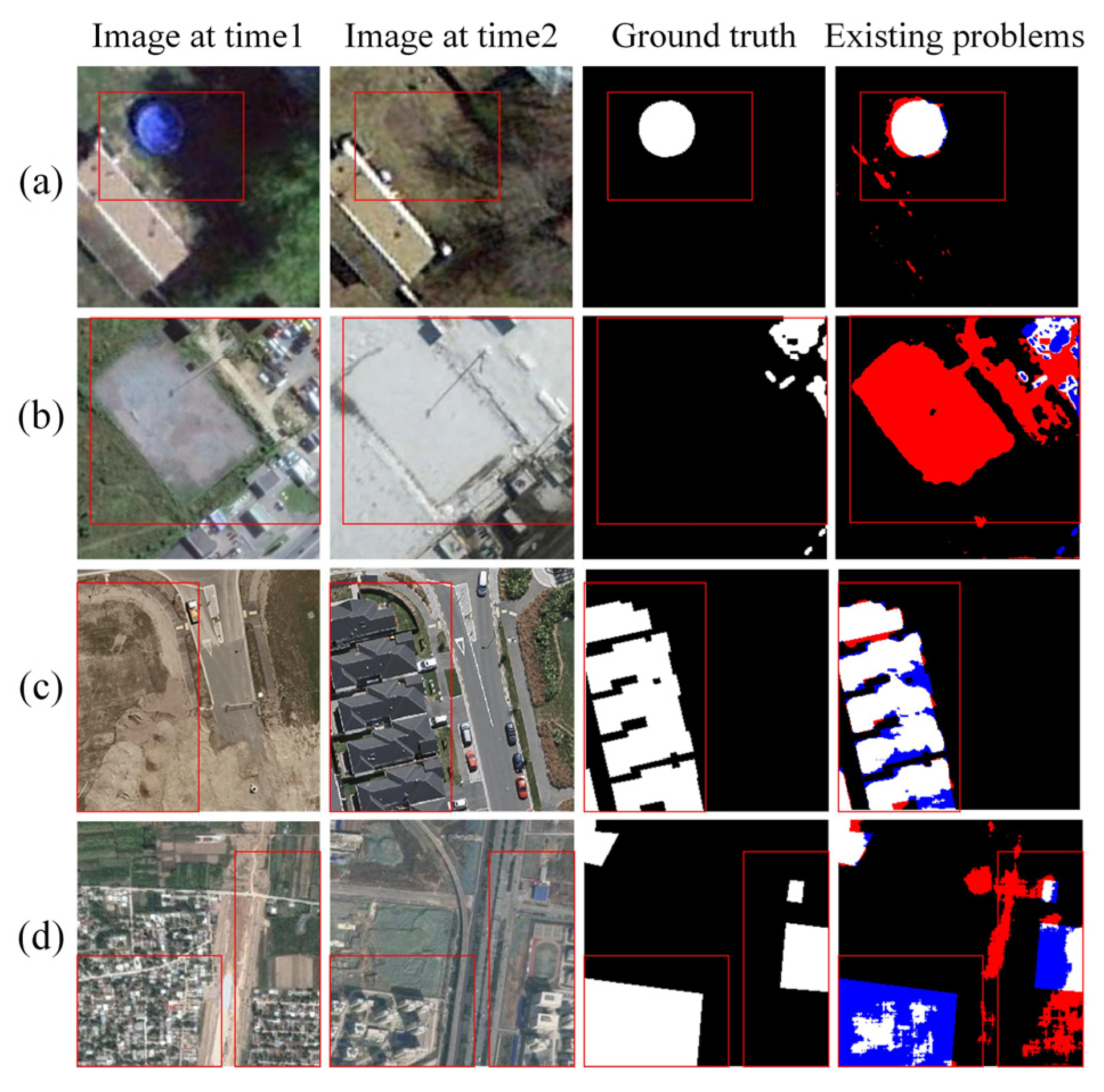
Although self-supervised learning provides an effective approach for enhancing feature representation, the existing methods still have significant deficiencies in adaptively handling sensor imaging differences, illumination (Figure 1a), and seasonal (Figure 1b) variations that cause pseudo changes. Furthermore, most existing RSICD networks tend to capture global representations while ignoring shallow fine-grained features, resulting in ineffective alignment of semantic representations between shallow and deep layers. This problem is particularly prominent in pixel-level RSICD, especially in building RSICD scenarios, where insufficient fine-grained feature representation often leads to blurred prediction boundaries, loss of local structures, and numerous false detections and missed detections (Figure 1c). Moreover, for remote sensing images with blurred boundaries, the model has difficulty capturing the contours of change areas during feature extraction, ultimately degrading the model’s overall performance (Figure 1d).

To alleviate these limitations, we propose a self-supervised pre-training style adaptation-guided RSICD network. During the pre-training stage, the cross-style self-supervised pre-training (CSSP) module was constructed to eliminate the influence of sensor imaging differences, illumination, and seasonal variations; in the downstream fine-tuning stage, the feature-domain multi-scale collaborative enhancement (FD-MSCE) module was designed; in addition, to address the blurred boundaries and missing details of the change areas caused by noise, clouds, fog, and insufficient resolution, the edge Gaussian aggregation (EGA) [26] module was introduced. The key contributions are summarized below:

• The self-supervised pre-training style adaptation-guided RSICD network was proposed. By constructing an unlabeled pre-training and downstream fine-tuning learning framework, the combination of style adaptation, self-supervised representation learning, and change detection was used to enhance the model’s detection ability under complex imaging conditions.
• The CSSP module was constructed, which effectively eliminates pseudo changes caused by sensor differences, illumination, and seasonal variations by combining generative adversarial networks and self-supervised pre-training techniques.
• The FD-MSCE module was designed to enhance fine-grained feature information and achieve cross-scale semantic alignment, effectively strengthening the identification of small-scale changes and improving prediction consistency.
• The EGA module was introduced to enhance the model’s ability to represent change boundaries, small targets, and local structural features, effectively resolving the ambiguity of change area boundaries and the lack of details, leading to improved overall detection performance.

2. Methodology

2.1. Architecture

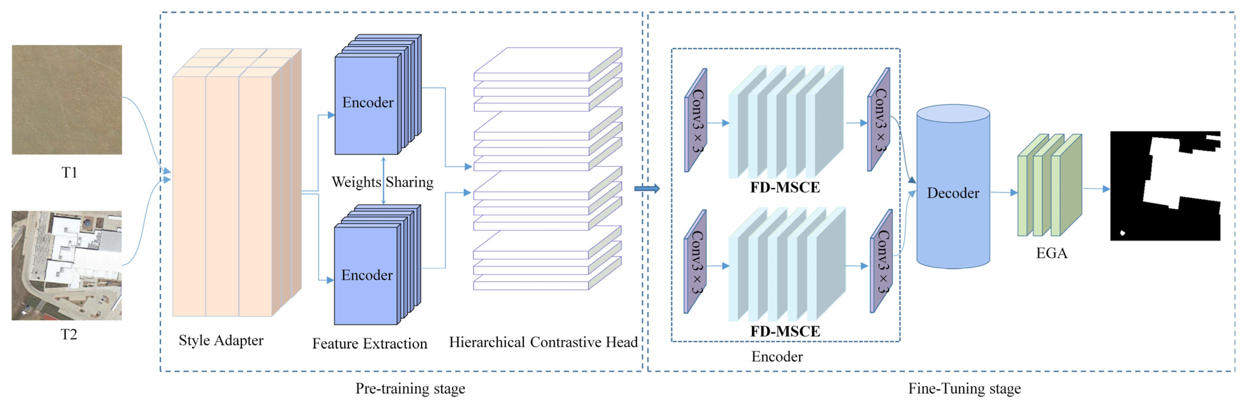
This paper proposes a self-supervised pre-training style adaptation-guided remote sensing image change detection (RSICD) network. Figure 2 illustrates the overall architecture of the proposed network. The architecture is organized into two phases: (1) the self-supervised pre-training phase; (2) the downstream fine-tuning phase.

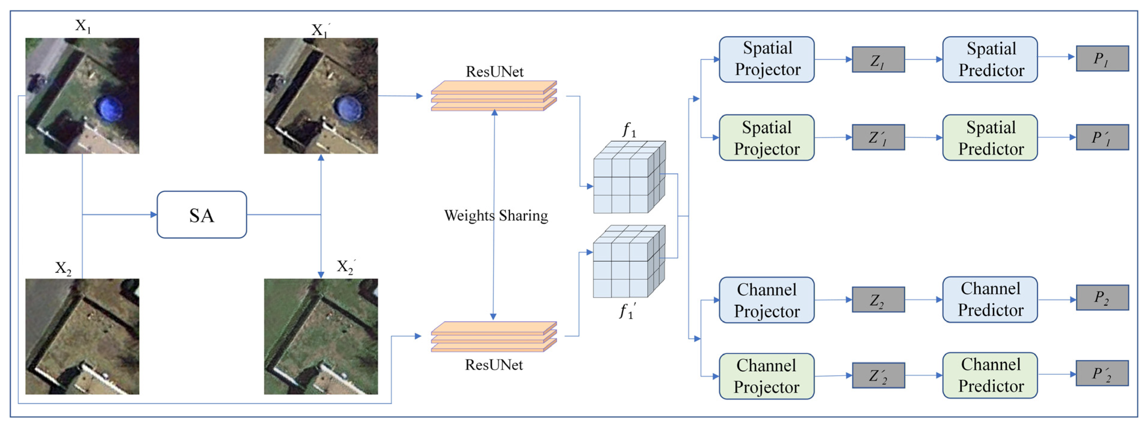
During the self-supervised pre-training phase, this study employs the constructed cross-style self-supervised pre-training (CSSP) module to alleviate the pseudo changes caused by illumination, seasons, and imaging differences. Firstly, the bi-temporal remote sensing images acquired at $T_1$ and $T_2$ are fed into the style adapter (SA), and the differences between the bi-temporal images are reduced through style transfer. Subsequently, two shared-weight encoders are used for feature extraction, and the extracted features are further input into the hierarchical contrast head [27], thereby allowing the model to learn stable structural and semantic representations while generating more distinctive pre-trained features for downstream change detection.

In the downstream change detection stage, the baseline model is constructed using a standard encoding–decoding structure. The Siamese network is adopted as the encoder, which consists of a dual-branch structure with shared weights, and each branch is composed of the same convolutional encoder. At the same time, the feature-domain multi-scale collaborative enhancement (FD-MSCE) module is used to enhance the fine-grained feature representation of the change areas at multiple scales, across multiple domains, and along multiple dimensions, ensuring that the model achieves a focused response to the features of the change areas. Finally, the edge Gaussian aggregation (EGA) module [28] is utilized to perform boundary smoothing and enhancement on the fused feature map after multi-scale feature fusion to retain key boundary information and avoid local structural loss and blurred boundaries in the final predictions caused by the absence of boundary features.

2.2. Cross-Style Self-Supervised Pre-Training Module

In RSICD, although images of the same geographical area are captured at different time points and may therefore exhibit substantial appearance discrepancies due to variation in illumination, weather, and seasons, these differences are not real changes, but they may cause the model to mistakenly identify the areas as changed, that is, to generate pseudo changes. To mitigate this problem, the CSSP module is constructed, and its architecture is illustrated in Figure 3. Firstly, a cycle-consistent generative adversarial network (CycleGAN) [26] is used as the SA, leveraging the style features of remote sensing images to train the SA for bidirectional mapping and generate naturally corresponding positive samples, thereby eliminating the distribution differences between the original bi-temporal images and alleviating the inter-domain deviations caused by different imaging conditions, illumination, and seasonal changes.

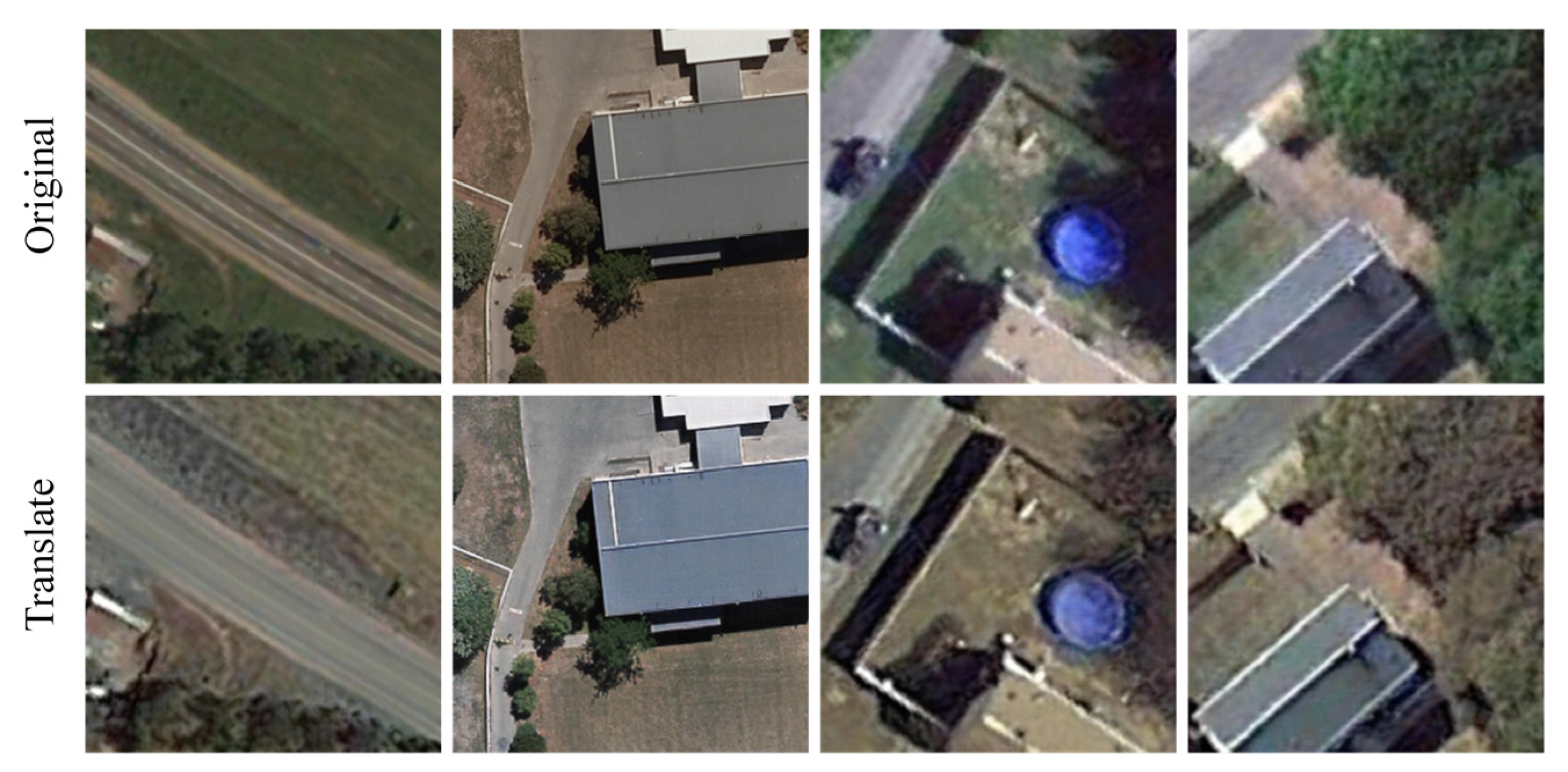
Specifically, the SA translates the $T_1$ image $X_1$ in the dataset into $X_1^{\prime }$, which is style-consistent with the $T_2$ image $X_2$ while preserving the original content of $X_1$. Meanwhile, it translates $X_2$ into $X_2^{\prime }$, whose style is consistent with that of $X_1$ while preserving the original content of $X_2$. It is worth noting that the SA primarily alters the image style, while largely preserving the spatial structures of the main objects and the overall layout of ground features within the scene (as shown in Figure 4). In particular, rooftops, shadows, vegetation, roads, and small-scale objects are well preserved. In the subsequent feature extraction stage, only $X_1$ and $X_1^{\prime }$ are fed into the two branches of the shared-weight ResUNet encoder for feature extraction, yielding the features $f_1$ and $f_1^{\prime }$, respectively. Subsequently, the hierarchical contrastive head [27] is utilized to fully explore the above features, $f_1$ and $f_1^{\prime }$. Firstly, the features go through the spatial projector and predictor:

$$\left\{\begin{array}{ll}{z}_1=\mathrm{Spa}\_\mathrm{Proj}(\mathrm{E}({\mathrm{x}}_1)),\hfill & p_1=\mathrm{Spa}\_\mathrm{Pred}(z_1)\hfill \\ z_1^{\prime }=\mathrm{Spa}\_\mathrm{Proj}(\mathrm{E}({\mathrm{x}}_1^{\prime })),\hfill & p_1^{\prime }=\mathrm{Spa}\_\mathrm{Pred}(z_1^{\prime })\hfill \end{array}\right.$$

(1)

where E(·) represents the encoder function used for extracting features, Spa_Proj(·) represents the spatial projector, Spa_Pred(·) represents the spatial predictor, $Z_1$ and $Z_1^{\prime }$ represent the intermediate feature encoding of the spatial branch, and $P_1$ and $P_1^{\prime }$ represent the encoding after the predictor.

Similarly, features $f_1$ and $f_1^{\prime }$ are respectively projected through the channel projector and the predictor:

$$\left\{\begin{array}{ll}{z}_2=\mathrm{Cha}\_\mathrm{Proj}(\mathrm{E}({\mathrm{x}}_1)),\hfill & p_2={\mathrm{Cha}\_\mathrm{Pred}(\mathrm{z}}_2)\hfill \\ z_2^{\prime }=\mathrm{Cha}\_\mathrm{Proj}(\mathrm{E}({\mathrm{x}}_1^{\prime })),\hfill & p_2^{\prime }={\mathrm{Cha}\_\mathrm{Pred}(\mathrm{z}}_2^{\prime })\hfill \end{array}\right.$$

(2)

where $\mathrm{E}\left(·\right)$ represents the encoder function used for extracting features, Cha_Proj(·) represents the channel projector, Cha_Pred(·) represents the channel predictor, $Z_2$ and $Z_2^{\prime }$ represent the intermediate encoding of the channel branches, and $P_2$ and $P_2^{\prime }$ represent the encoding after the channel predictor.

To promote representation consistency across the two branches, a negative cosine similarity loss is employed:

$$D\left(z_1,p_1^{\prime }\right)=-〈{\displaystyle \frac{z_1}{{‖z_1‖}_2}},{\displaystyle \frac{p_1^{\prime }}{{‖p_1^{\prime }‖}_2}}〉$$

(3)

Loss function for the spatial branches [27]:

$${\mathcal{L}}_{\mathrm{Spa}}={\displaystyle \frac{D\left(z_1,p_1^{\prime }\right)}{2}}+{\displaystyle \frac{D\left(z_1^{\prime },p_1\right)}{2}}$$

(4)

Loss function for the channel branches [27]:

$${\mathcal{L}}_{\mathrm{Cha}}={\displaystyle \frac{D\left(z_2,p_2^{\prime }\right)}{2}}+{\displaystyle \frac{D\left(z_2^{\prime },p_2\right)}{2}}$$

(5)

During this process, no labels are introduced. Instead, a hierarchical cross-comparison mechanism is incorporated into both branches to guide model optimization. The overall loss function of the hierarchical contrastive head is then formulated as a weighted sum of the spatial loss and channel loss:

$$\mathcal{L}=\alpha \cdot {\mathcal{L}}_{\mathrm{Spa}}+(1-\alpha )\cdot {\mathcal{L}}_{\mathrm{Cha}}$$

(6)

Among these, α denotes the weight parameter of the spatial branch and is set to 0.5 in this study.

2.3. Feature-Domain Multi-Scale Collaborative Enhancement

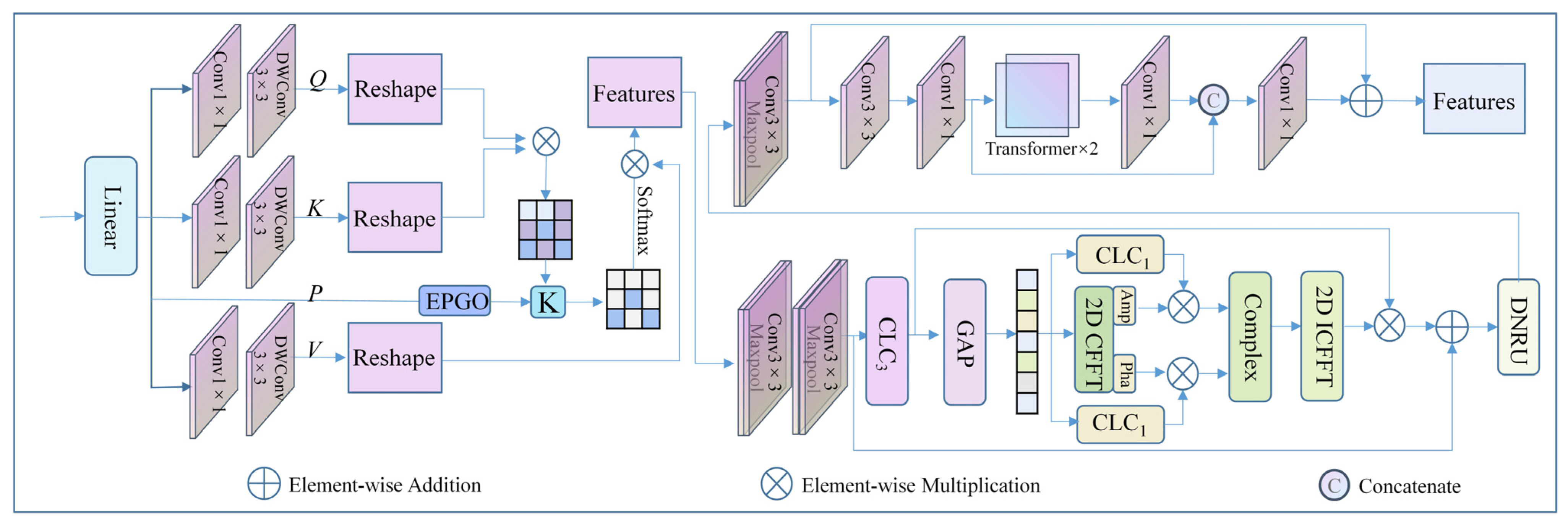
To address the model’s tendency to lose shallow, fine-grained information during downsampling and to lack effective multi-scale feature fusion and semantic alignment, the FD-MSCE module is designed (as shown in Figure 5). Firstly, following the sparse prompt channel self-attention mechanism proposed in [29], point-wise convolution and deep convolution aggregation, cross-pixel channel information is generated to form feature matrices for the query (Q), key (K), and value (V). Subsequently, the reshaped Q and K are subjected to element-wise multiplication to obtain the attention matrix $M\in R^{C\times C}$, which prevents possible false noise during denoising. A top-k mechanism is introduced to filter and retain the key information in the attention matrix. At the same time, the efficient prompt guiding operator is used to dynamically generate prompt vectors based on the input features, guiding the K value for adaptive modulation to achieve the dynamic selection of the attention matrix. The corresponding computation is formulated as follows:

$${\Omega }_i^{(k)}=\arg \underset{S\subset \{1,\dots ,N\}}{\max }{\displaystyle \sum _{j\in S}{M}_{ij}}$$

(7)

$${\Omega }^{(k)}=\left\{{\Omega }_1^{(k)},{\Omega }_2^{(k)},\dots ,{\Omega }_N^{(k)}\right\}$$

(8)

$${\left[M_k\right]}_{ij}=\left\{\begin{array}{l}1, if j\in {\Omega }_i^{(k)}\hfill \\ 0, otherwise. \hfill \end{array}\iff M_{ij}\in {\mathrm{Top}}_k\left(M_{i,:}\right)\right.$$

(9)

where ${\Omega }_i^K$ denotes the set of column indices associated with the top-k largest attention scores in the i-th row of $M$. The processing procedure of the sparse prompt channel self-attention mechanism is as follows:

$$SPC-SA=Soft\max \left(T_k\left({\displaystyle \frac{Q{K}^T}{\sqrt{d}}}\right)\right)V$$

(10)

where $T_K\left(·\right)$ represents the top-k selection operator guided by the efficient prompt guiding operator, and $1/\sqrt{d}$ is used to scale the dot product between Q and K, preventing excessively large attention logits and stabilizing the subsequent Softmax operation. Finally, all the outputs of the multi-head attention are concatenated and projected through a linear layer to obtain the feature map. After performing convolution and downsampling operations on the obtained feature map, the Fourier residual channel attention block [30] is employed, which jointly integrates the Residual-in-Residual (RIR) structure and Fourier channel attention (FCA) for feature enhancement. Here, RIR enables the encoder to pay more attention to high-frequency components, whereas FCA captures the statistical information between channels, thereby improving the model’s capability to distinguish global information. Feature X obtains a global vector representation through global average pooling, then undergoes a fast Fourier Transform in the channel dimension, and enhances the amplitude and phase information of feature X. Subsequently, the inverse Fourier Transform is applied, and two residual connections are constructed. Finally, $DNRU\left(·\right)$ is used for further feature refinement and scale restoration to obtain the output result y:

$$x^c=CFFT\left(GAP\left(CL{C}_3(x)\right)\right)$$

(11)

$$a^x=Amp\left(x^c\right),p^x=Pha\left(x^c\right)$$

(12)

$$a^{xc}=a^x\times GAP\left(CL{C}_1(x)\right)$$

(13)

$$p^{xc}=p^x\times GAP\left(CL{C}_1(x)\right)$$

(14)

$$x^{ic}=ICFFT\left(Complex\left(a^{xc},p^{xc}\right)\right)\times CL{C}_3(x)+x$$

(15)

$$y=DNRU\left(x^{ic}\right)$$

(16)

where, $x^c$ denotes the channel-domain frequency feature; $a^{xc}$ and $p^{xc}$ denote the amplitude and phase components modulated by the channel-wise statistical information, respectively. Next, the convolution with the Vision Transformer [31] is adopted. The 3 × 3 convolution and the 1 × 1 convolution are applied to the processed feature y to establish local context correlations. Then, using the stacking and unstacking operations of the Transformer, a bridge is established between the convolution operation and the Transformer operation. The self-attention mechanism is described as follows:

$${\mathcal{A}}_{\mathrm{ViT}}(\mathrm{q},\mathrm{k},\mathrm{v})=\mathrm{softmax}\left({\displaystyle \frac{{\mathrm{qk}}^T}{\sqrt{D_{\mathrm{h}}}}}\right)v$$

(17)

where N denotes the total number of image patches, while D indicates the embedding dimension of each patch token. When using m self-attention heads, the feature dimension of each head is defined as D/m. Additionally, to alleviate the information loss of small-scale targets in the feature extraction process of remote sensing images, a skip connection operation is introduced. Through the hybrid architecture of convolution and Transformer, the model can simultaneously capture local texture features and context information, and can more precisely align the fine areas of actual ground changes.

2.4. Edge Gaussian Aggregation

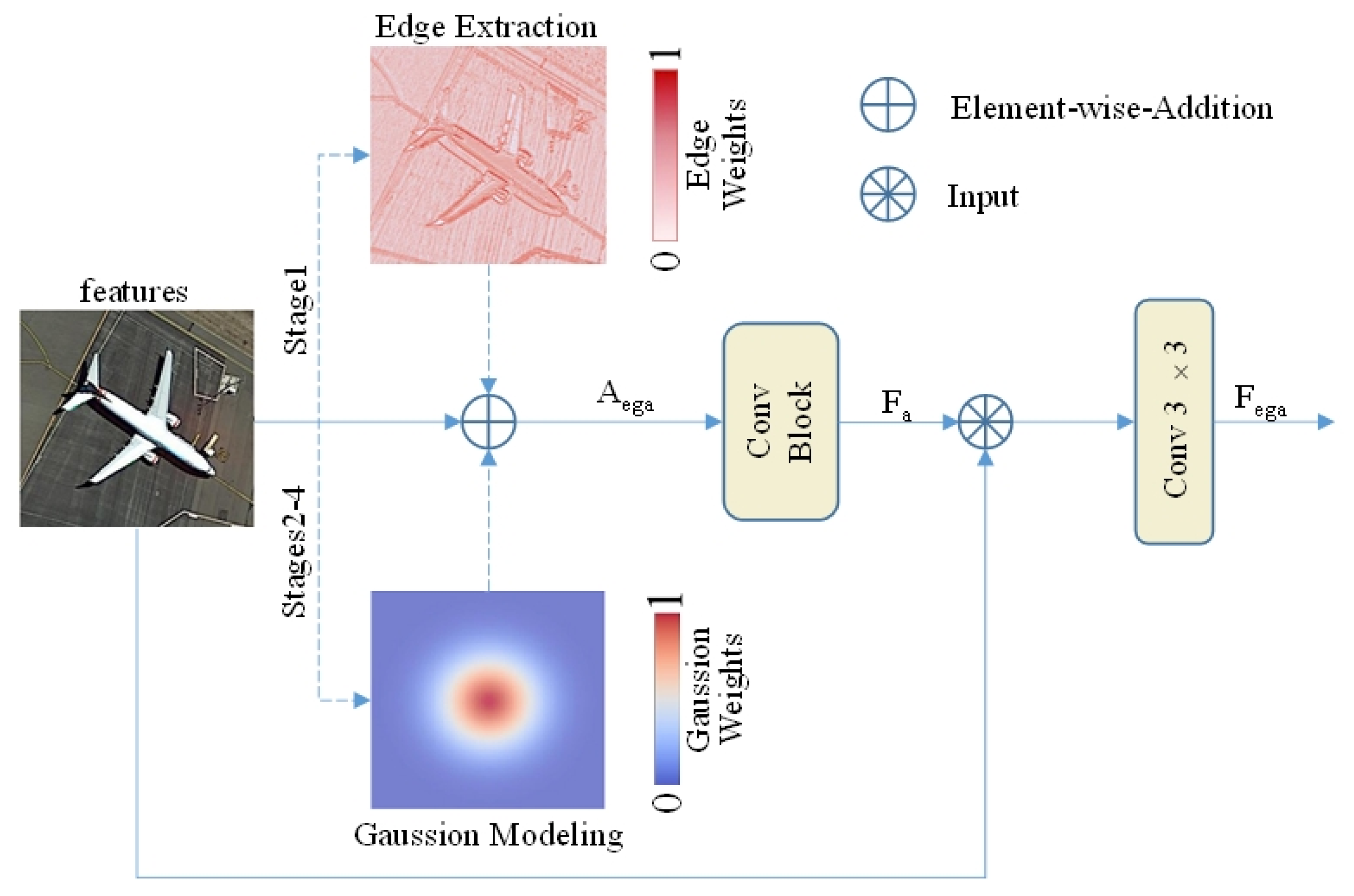
To address the issues of blurred domain boundaries and lost details in remote sensing images caused by noise, clouds, and insufficient resolution, this paper introduces the EGA module [28] (illustrated in Figure 6). Its operational procedure is described below:

The EGA processes the input features $F_{in}$ through a selection mechanism, which selects either the boundary extraction or Gaussian modeling module depending on the stage:

$$A_{\mathrm{ega} }=\left\{\begin{array}{ll}{A}_{\mathrm{edge} }\left(F_{\mathrm{in} }\right),\hfill & \mathrm{if} \mathrm{Stage} =1,\hfill \\ A_{\mathrm{gauss} }\left(F_{\mathrm{in} }\right),\hfill & \mathrm{otherwise}. \hfill \end{array}\right.$$

(18)

where $A_{edga}\left(\cdot \right)$ and $A_{gauss}\left(\cdot \right)$ denote the edge extraction and Gaussian-modeling operation, respectively. After processing by the selection mechanism, the sum of $A_{ega}$ and $F_{in}$ is added together, and then this sum is input into a three-layer convolution block to enhance the feature representation ability:

$$F_{\mathrm{temp} }={\mathrm{Conv}}_{2D}^{3\times 3}\left(\mathrm{AN}\left({\mathrm{Conv}}_{2D}^{1\times 1}\left(F_{\mathrm{in} }+A_{\mathrm{ega} }\left(F_{\mathrm{in} }\right)\right)\right)\right)$$

(19)

where $AN\left(\cdot \right)$ denotes the activation-normalization layer. The output of the convolution block is:

$$\mathrm{Conv}\_\mathrm{Block}\left(F_{in}\right)=\mathrm{Norm}\left({\mathrm{Conv}}_{2D}^{1\times 1}\left(\mathrm{AN}\left(F_{temp}\right)\right)\right)$$

(20)

Finally, the result $F_a$ of the convolution block, which denotes the modulation feature used to adaptively reweight the $F_{in}$, is fused with $F_{in}$ through element-wise multiplication and residual addition. A 3 × 3 convolution is then applied to generate the final module output:

$$F_{ega}={\mathrm{Conv}}_{2D}^{3\times 3}\left(\left(F_{in}\otimes F_a\right)+F_{in}\right)$$

(21)

2.5. Loss Function

The loss function used in this paper is described as follows. In the downstream change detection network, to mitigate the impact of sample imbalance, a hybrid loss function composed of weighted cross-entropy loss ($L_{WCE}$) and dice loss ($L_{Dice}$) [32] is used, and it is defined as:

$$\mathcal{L}(y,\hat{y})={\mathcal{L}}_{\mathrm{WCE} }+{\mathcal{L}}_{\mathrm{Dice} }$$

(22)

$${\mathcal{L}}_{\mathrm{WCE}}=-\omega \cdot \hat{y}\cdot \log (y)-(1-\hat{y})\cdot (\log (1-y))$$

(23)

$${\mathcal{L}}_{\mathrm{Dice} }=1-{\displaystyle \frac{2\cdot \hat{y}\cdot \mathrm{softmax}(y)}{\hat{y}+\mathrm{softmax}(y)}}$$

(24)

Among these, ω is the weight parameter of the positive sample. In this experiment, ω is set to 1, and y and $\hat{y}$ are the variation graphs calculated by the baseline network and the real changed map, respectively.

3. Experiments and Analysis

3.1. Dataset Description

Four publicly available change detection datasets, namely LEVIR [33], WHU [34], DSIFN [35] and CDD [36], were employed to assess the performance of the proposed method. A summary of these datasets is provided in

Table 1. Overview of the four experimental datasets.

Dataset	Resolution	Sample Size	Number of Samples	Train/Val/Test
LEVIR	0.5 m	256 × 256	10,192	7120/1024/2048
WHU	0.3 m	256 × 256	7434	5947/743/744
DSIFN	2 m	256 × 256	15,952	14,400/1360/192
CDD	0.03–1 m	256 × 256	16,000	10,000/3000/3000

. For the LEVIR dataset, 637 bi-temporal image pairs and their associated labels were partitioned into training, validation, and testing subsets using a 7:1:2 ratio. Subsequently, each image pair and its corresponding labels were cropped in a synchronized manner into non-overlapping patches of 256 × 256 pixels. For the WHU dataset, the original spatially non-overlapping geographical regions were divided into training, validation, and test sets at a ratio of 8:1:1, after which the images and labels in each subset were synchronously cropped into patches of 256 × 256 pixels. Following the original partitioning protocol of the DSIFN dataset, the data from Beijing, Chengdu, Shenzhen, Chongqing, and Wuhan were used for training and validation, while the data from Xi’an were used as an independent test set. The CDD dataset comprises 16,000 bi-temporal image pairs, each with a spatial size of 256 × 256 pixels. These samples are allocated to the training, validation, and testing subsets in quantities of 10,000, 3000, and 3000, respectively.

3.2. Evaluation Metrics

To quantitatively assess the proposed method, four commonly used indicators, namely Precision (P), Recall (R), F1-score (F1), and Intersection over Union (IoU), were calculated based on the generated predicted images and the true change images for evaluating accuracy.

$$\mathrm{Precision}={\displaystyle \frac{TP}{TP+FP}}$$

(25)

$$\mathrm{Recall}={\displaystyle \frac{TP}{TP+FN}}$$

(26)

$$F1=2\times {\displaystyle \frac{\mathrm{Precision}\times \mathrm{Recall}}{\mathrm{Precision}+\mathrm{Recall}}}$$

(27)

$$IoU={\displaystyle \frac{TP}{TP+FN+FP}}$$

(28)

where TP, FP, and FN denote the numbers of true positive, false positive, and false negative pixels, respectively.

3.3. Experimental Setup

Table 2. Hardware and software configuration.

Operating Environment		CSSP Pretraining		Downstream Fine-Tuning
		Hyperparameter Setting
System	Windows11	Batch	8	4
CPU	Intel(R) Core (TM) i7-13700KF	epoch	100
GPU	NVIDIA GeForceRTX3090 (24 G)	Initial Learning Rate	0.001
Python	3.80	Optimization	SGD	AdamW
CUDA	11.6	weight decay	0.0001	0.01
PyTorch	1.13.1	momentum	0.9	0.9, 0.999

summarizes the experimental environment and the main hyperparameter settings for CSSP pre-training and downstream fine-tuning.

3.4. Comparison Methods

To evaluate the proposed method, extensive comparisons were conducted with advanced remote sensing image change detection (RSICD) methods. The comparison methods included: STADE-CDNet [37], BIFA [38], MS-Former [39], TransWCD [40], ACWCD [41], and KD-MSI [42]. To ensure the fairness of the comparative experiments, all selected competing methods were reimplemented in our local experimental environment using their publicly available source codes, and the results reported in the tables were not directly taken from the original publications. All methods used the same training, validation, and test sets, as well as identical input data, image sizes, and evaluation protocols.

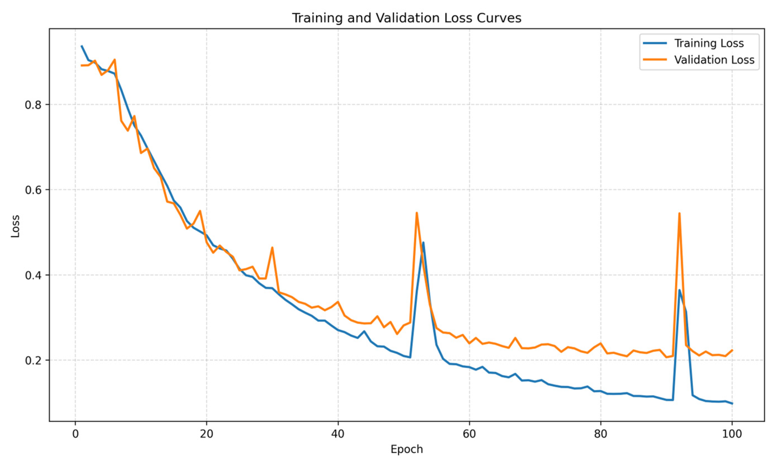
3.5. Training and Validation Loss Analysis

To further evaluate the convergence behavior of the proposed model and investigate potential overfitting or underfitting, the training and validation losses over 100 epochs are shown in Figure 7. Both losses decreased rapidly during the early training stage and exhibited generally consistent trends, demonstrating the model’s ability to extract distinctive feature representations while maintaining a stable convergence process. Beyond roughly 60 epochs, the training loss decreased further, whereas the validation loss remained nearly constant at a low value. This demonstrated that the model had been sufficiently trained and did not exhibit evident underfitting. Although the gap between the training and validation losses slightly increased during the later stage, the validation loss did not show a sustained upward trend, indicating only mild overfitting. Two temporary fluctuations were observed at approximately epochs 52 and 92; however, the losses quickly returned to their previous trends, suggesting short-term optimization variations rather than model divergence. Overall, the proposed model demonstrated satisfactory convergence and generalization performance.

3.6. Experimental Results on the DSIFN Dataset

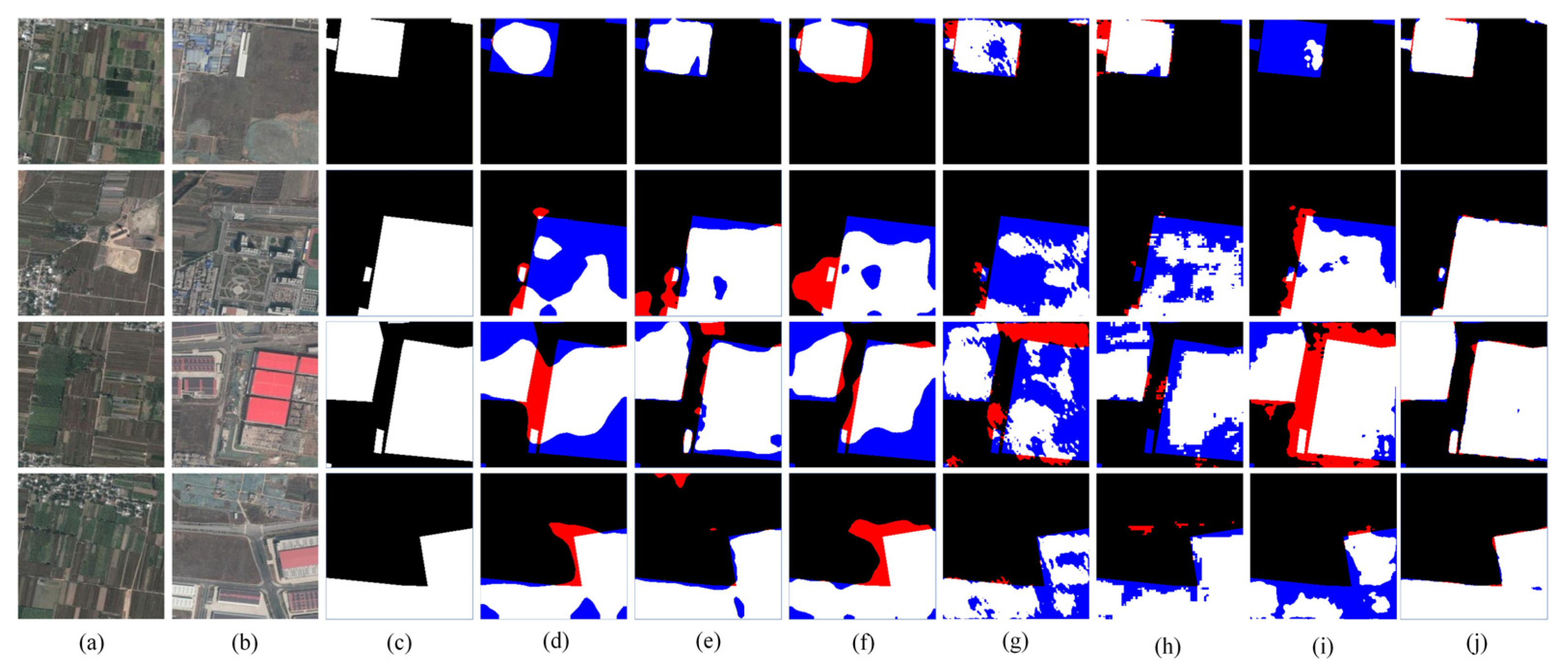
As reported in

Table 3. Quantitative evaluation results on the DSIFN dataset.

Methods	DSIFN
	P (%)	R (%)	F1 (%)	IoU (%)
MS-Former	74.08	59.13	65.77	48.99
TransWCD	43.25	72.40	54.15	37.13
ACWCD	61.57	51.02	55.80	38.70
KD-MSI	85.99	77.30	81.42	68.66
STADE-CDNet	71.03	48.63	57.73	40.58
BIFA	78.72	65.85	71.71	55.90
Ours	92.51	91.87	92.19	85.51

Bold represents the best, and underline represents the 2nd-best.

, the proposed method achieved the highest values for the P, R, F1, and IoU indicators on the DSIFN dataset, reaching 92.51%, 91.87%, 92.19%, and 85.51%, respectively. Compared to the suboptimal comparison method KD-MSI, it improved by 6.52%, 14.57%, 10.77%, and 16.85%, respectively. Among all the comparison methods, TransWCD did not show significant advantages on this dataset. STADE-CDNet, MS-Former, and ACWCD performed relatively evenly across all indicators. In contrast, the proposed method demonstrated optimal performance.

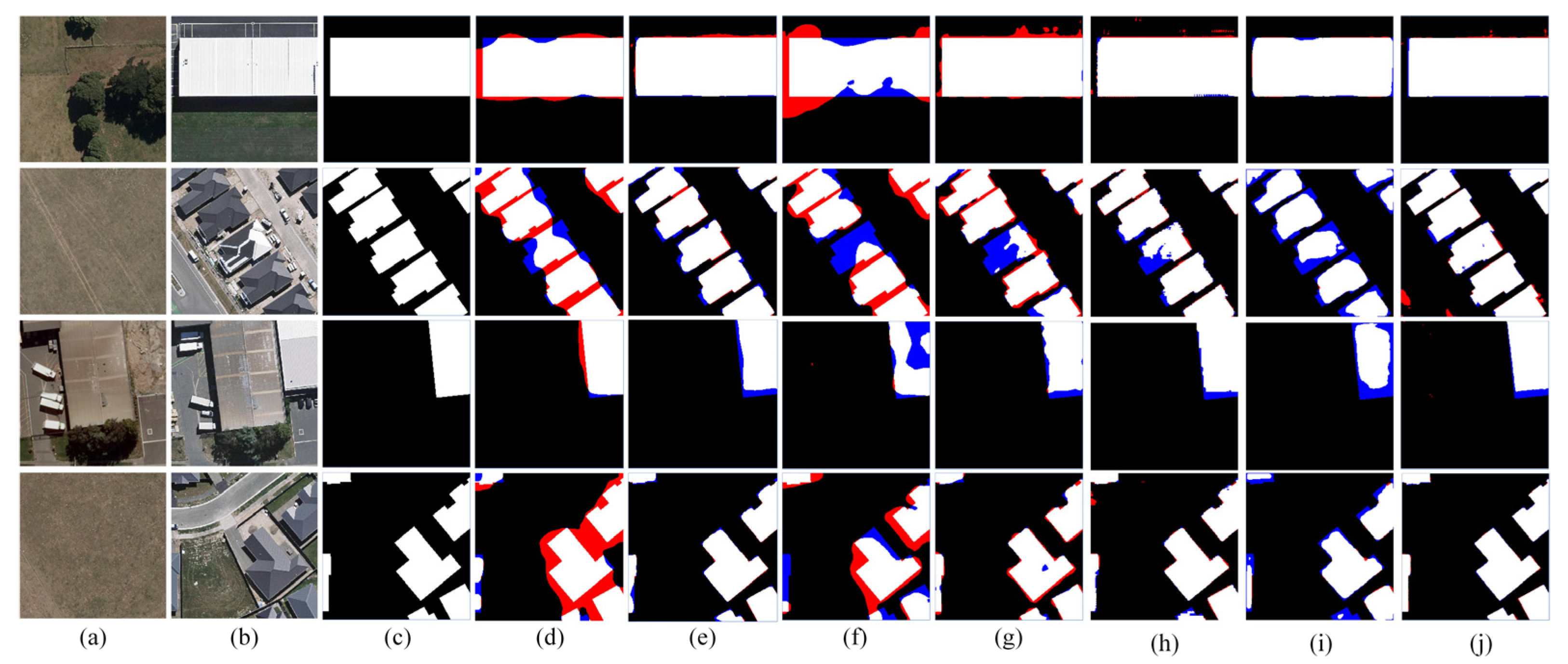
Figure 8 shows the visualization of the experimental results on the DSIFN dataset. The proposed method had the fewest false detections (represented in red) and missed detections (represented in blue) in the experimental results and was closest to the ground truth. Among the comparison methods, MS-Former, TransWCD, BIFA, STADE-CDNet, and ACWCD all had certain limitations to varying degrees. Among them, the detection results of MS-Former still showed deficiencies in the overall recognition of the change areas and boundary response, which further led to unsatisfactory clarity and continuity of the change boundaries. In contrast, KD-MSI produced relatively fewer false detections and missed detections, and the boundary detection performance was also improved. However, there were still some false detections in the boundary detection of the change areas. Specifically, the proposed method performed best in boundary detection and the recognition of the change areas, and the change boundary was clearer.

3.7. Experimental Results on the LEVIR Dataset

The results presented in

Table 4. Quantitative evaluation results on the LEVIR dataset.

Methods	LEVIR
	P (%)	R (%)	F1 (%)	IoU (%)
MS-Former	71.40	85.49	77.81	63.68
TransWCD	46.34	62.47	53.21	36.25
ACWCD	53.03	80.01	63.79	46.83
KD-MSI	97.17	61.60	75.40	60.51
STADE-CDNet	88.25	59.35	70.79	55.00
BIFA	91.62	87.32	89.42	80.86
Ours	90.59	89.54	90.06	81.92

Bold represents the best, and underline represents the 2nd-best.

demonstrate that the proposed method achieved superior performance compared with the other methods on the LEVIR dataset. Although its P was lower than that of KD-MSI and BIFA, it obtained the highest results in terms of R, F1, and IoU, indicating that KD-MSI and BIFA did not fully cover the change areas and still exhibited some missed detections. By comparison, the proposed method achieved the highest R and IoU. A high R indicates a stronger capability to reduce false detections, while a higher IoU indicates a more comprehensive coverage of the actual situation. In summary, the proposed method provides more accurate predictions and better spatial consistency, indicating that the model has stronger representational and discrimination capabilities in extracting change features and preserving spatial details.

Figure 9 presents the qualitative comparison results on the LEVIR dataset. The model proposed produces more accurate change areas and demonstrates better visual performance than the competing methods. In contrast, KD-MSI, MS-Former, and BIFA also demonstrate strong overall detection capabilities, with relatively fewer false detections and missed detections in their predictions. Compared to KD-MSI, MS-Former, and BIFA, the boundary detection effect of this method is better, and the change detection details are also more outstanding, proving the effectiveness of the method proposed.

3.8. Experimental Results on the WHU Dataset

As reported in

Table 5. Quantitative evaluation results on the WHU dataset.

Methods	WHU
	P (%)	R (%)	F1 (%)	IoU (%)
MS-Former	88.78	88.09	88.43	79.27
TransWCD	66.27	59.16	62.51	45.47
ACWCD	73.99	79.57	76.68	62.18
KD-MSI	96.12	82.35	88.70	79.70
STADE-CDNet	96.67	56.95	71.86	55.86
BIFA	88.22	84.23	86.18	75.72
Ours	90.59	90.18	90.39	82.46

Bold represents the best, and underline represents the 2nd-best.

, the proposed method achieved better results across all evaluation indicators than the competing approaches on the WHU dataset. However, in terms of P, it was lower than that of KD-MSI and STADE-CDNet. Nevertheless, the R and IoU of KD-MSI and STADE-CDNet were significantly lower than those of the proposed method, indicating that the proposed method is more effective at detecting change areas and that its predictions show greater agreement with the ground truth maps. Overall, the proposed method delivers the best comprehensive performance on the WHU dataset.

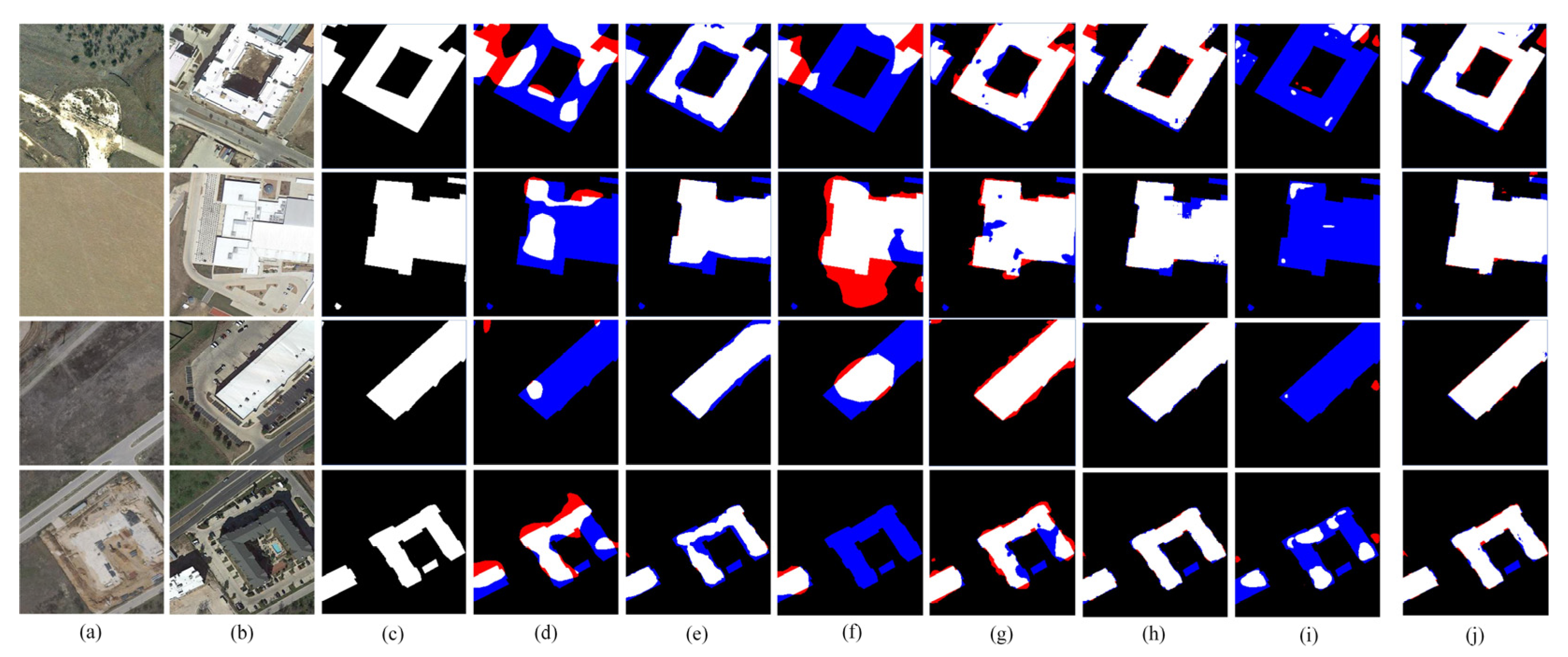
The visual comparison results obtained on the WHU dataset are illustrated in Figure 10. KD-MSI, MS-Former, and BIFA demonstrate relatively strong detection performance, but there are still some false detections (indicated in red) and missed detections (indicated in blue). In contrast, the proposed method generates more accurate detection results with clearer delineation of the change areas. Its boundaries are more sharply defined, and it performs more stably in complex backgrounds.

4. Discussion

4.1. Robustness Experiment

To further evaluate the detection robustness of the proposed method under diverse change types and complex scene conditions, we conducted additional experiments on the CDD dataset. Compared with DSIFN, LEVIR, and WHU, this dataset not only includes changes in buildings, but also changes caused by human and natural factors such as vehicles and roads. Therefore, it provides a more diverse and challenging benchmark for evaluating the performance of the model under complex seasonal, radiometric, and scene variations. In addition to the conventional evaluation indicators, a pixel-level confusion matrix (Ss shown in

Table 6. Pixel-Level confusion matrix on the CDD test set.

Ground Truth/Prediction	Unchanged	Changed
Unchanged	TN = 170,325,089	FP = 1,180,820
Changed	FN = 2,089,574	TP = 23,012,517

) reporting the numbers of TP, TN, FP, and FN is further provided to enable a more comprehensive assessment of the model’s detection performance.

The results in

Table 7. Quantitative evaluation results on the CDD dataset.

Methods	CDD
	P (%)	R (%)	F1 (%)	IoU (%)
MS-Former	75.36	62.13	68.11	51.64
TransWCD	31.54	52.45	39.39	24.53
ACWCD	62.10	34.95	44.73	28.81
KD-MSI	97.93	67.72	80.07	66.67
STADE-CDNet	97.86	57.15	72.15	56.44
BIFA	92.34	92.32	92.33	85.75
ours	95.12	91.68	93.37	87.56

Bold represents the best, and underline represents the 2nd-best.

show that the proposed method achieved significantly better results than the competing methods in terms of F1 and IoU on the CDD dataset, achieving 93.37% and 87.56%, respectively, demonstrating a more balanced and stable detection performance.

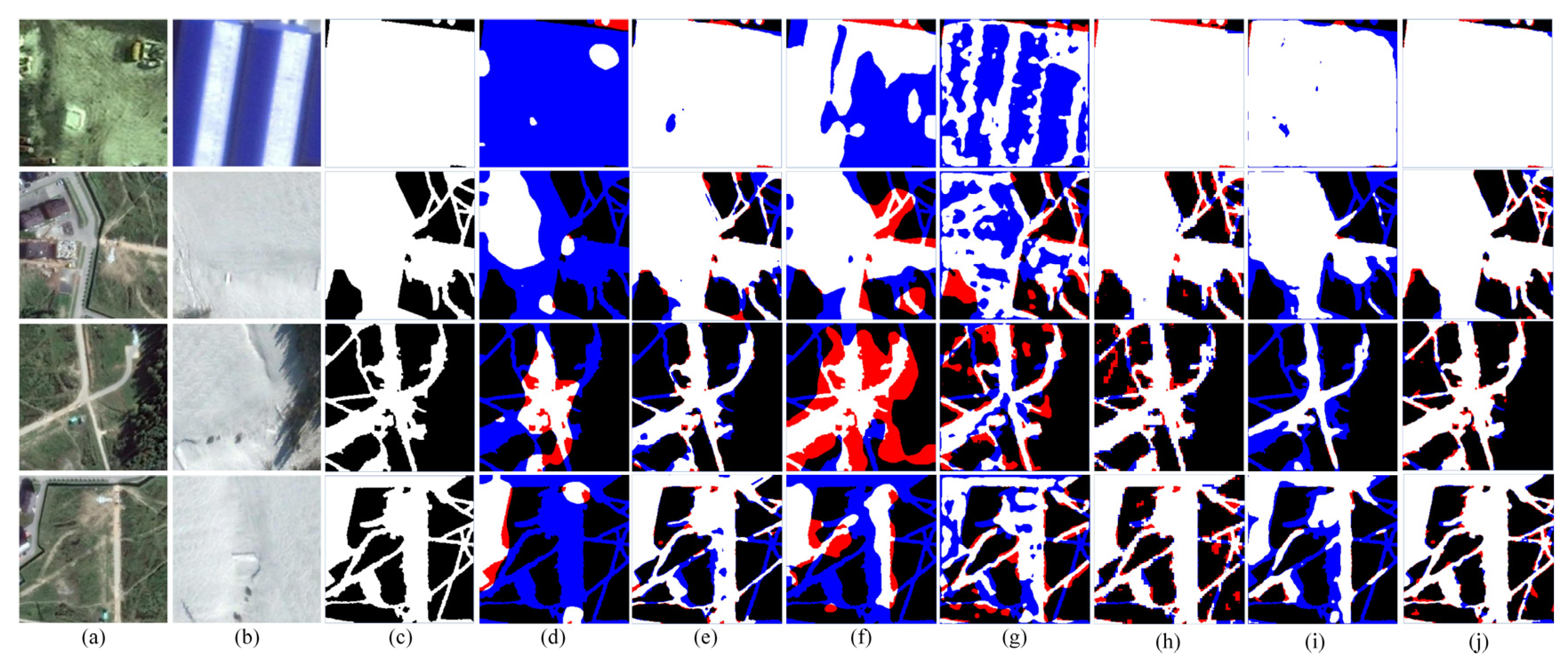
Figure 11 illustrates representative qualitative comparisons on the CDD dataset. ACWCD, TransWCD, MS-Former, and STADE-CDNet exhibited missed and false detections in some areas and showed deficiencies in the completeness and boundary clarity of the change areas. KD-MSI and BIFA demonstrated stable performance, but they also exhibited certain missed detections and a few false detections. In contrast, under the influence of snow cover and complex backgrounds, the proposed method accurately detected the change areas, with sharp boundary contours, and the predicted change areas were highly consistent with the real change areas. The proposed method effectively mitigated interference from pseudo changes and demonstrated stronger robustness and visual consistency.

4.2. Ablation Experiment

To further evaluate the model’s ability to detect change boundaries, the Boundary F1 score was added as a supplementary evaluation indicator in the ablation experiments:

$$\mathrm{Boundary} \mathrm{F}1=2\times {\displaystyle \frac{\mathrm{BP}\times \mathrm{BR}}{\mathrm{BP}+\mathrm{BR}}}$$

(29)

where BP denotes boundary precision, defined as the proportion of predicted boundary pixels located within a distance of no more than two pixels from the ground-truth boundary to all predicted boundary pixels; BR denotes boundary recall, defined as the proportion of ground-truth boundary pixels located within a distance of no more than two pixels from the predicted boundary to all ground-truth boundary pixels.

To verify the effectiveness of the style adapter (SA), this paper conducted experiments on the WHU dataset, including models with SA and without SA, and transferred the pre-trained models to the baseline network for fine-tuning. The ablation experiment results are reported in

Table 8. Quantitative evaluation results of SA ablation in WHU.

Modules	WHU
SA	P (%)	R (%)	F1 (%)	IoU (%)	Boundary F1 (%)
	89.46	85.57	87.47	77.74	63.27
√	90.59	90.18	90.39	82.46	65.83

Bold represents the best.

. It can be seen that after introducing SA, the model exhibited substantial gains across all five evaluation indicators. Meanwhile, the improvement in the Boundary F1 score further demonstrated that SA enhanced the model’s ability to accurately detect change boundaries. This indicated that SA could effectively alleviate pseudo changes between bi-temporal remote sensing images caused by illumination, imaging conditions, and seasonal differences. It helped to enhance the model’s response ability to real change areas and reduce missed detections and false detections.

To verify the effectiveness of the cross-style self-supervised pre-training (CSSP) module, ablation experiments were conducted on the WHU dataset to evaluate model variants incorporating or excluding the CSSP module. The experimental results are summarized in

Table 9. Quantitative evaluation results of CSSP ablation in WHU.

Modules	WHU
CSSP	P (%)	R (%)	F1 (%)	IoU (%)	Boundary F1 (%)
	83.80	88.90	86.27	75.86	52.55
√	90.59	90.18	90.39	82.46	65.83

Bold represents the best.

, which demonstrate that by incorporating the CSSP module, the proposed model achieved significant improvements in five evaluation indicators. These improvements demonstrated that the CSSP module could learn more robust cross-style feature representations during the pre-training stage, thereby enhancing the model’s ability to distinguish actual changes from stable areas and improving its overall detection accuracy.

To verify the effectiveness and stability of SA in scenarios with substantial seasonal variations, ablation experiments with and without SA were conducted on the CDD dataset, and the results are presented in

Table 10. Quantitative evaluation results of SA ablation in CDD.

Modules	CDD
SA	P (%)	R (%)	F1 (%)	IoU (%)	Boundary F1 (%)
	92.16	86.67	89.33	80.72	54.63
√	95.12	91.68	93.37	87.56	72.98

Bold represents the best.

. After introducing SA, the model achieved improvements in all five evaluation indicators. These results demonstrated that SA could alleviate style interference caused by seasonal variations, suppress pseudo change responses, and reduce missed detections of real change regions. Overall, SA maintained good stability and robustness in complex scenarios.

To examine the effectiveness and robustness of CSSP under complex conditions involving pronounced seasonal differences, ablation studies were carried out on the CDD dataset by comparing models with and without this module. The corresponding results are summarized in

Table 11. Quantitative evaluation results of CSSP ablation in CDD.

Modules	CDD
CSSP	P (%)	R (%)	F1 (%)	IoU (%)	Boundary F1 (%)
	90.16	77.68	83.46	71.61	32.20
√	95.12	91.68	93.37	87.56	72.98

Bold represents the best.

. After introducing CSSP, the model achieved improvements in all five evaluation indicators. These results indicated that CSSP could not only reduce pseudo changes caused by seasonal variations and illumination differences, but also decrease missed detections and false detections of real changes while improving the completeness of detected change regions. Therefore, the experimental results on the CDD dataset demonstrated that CSSP maintained good stability and robustness in complex scenarios with substantial seasonal variations.

To investigate the individual contribution of each component in the proposed method, comprehensive ablation studies were performed on the WHU dataset. Each module was successively incorporated into the baseline model in a permutation and combination manner, and the experimental results were quantitatively evaluated.

Table 12. The ablation experiment results of the modules proposed in WHU.

Modules		WHU
FD-MSCE	EGA	P (%)	R (%)	F1 (%)	IoU (%)	Boundary F1 (%)
		82.07	86.06	84.01	72.44	53.06
√		87.55	81.70	84.52	73.19	41.73
	√	88.12	90.78	89.43	80.88	63.67
√	√	90.59	90.18	90.39	82.46	65.83

Bold represents the best.

shows the changes in model performance after the gradual introduction of the modules.

As summarized in Table 12, the baseline model achieved a P of 82.07%, an F1 of 84.01%, and an IoU of 72.44%. When the feature-domain multi-scale collaborative enhancement (FD-MSCE) module was added, the P, F1, and IoU of the model improved, indicating that this module enhanced the model’s discrimination ability for the change areas, effectively reduced false detections, and improved overall detection accuracy. However, R and Boundary F1 decreased, suggesting that the model became more conservative and exhibited limited performance in boundary delineation. There were still certain missed detections in identifying all the change areas. After adding the edge Gaussian aggregation (EGA) module, all five evaluation indicators of the model significantly improved, indicating that the EGA module helped the model capture the change areas more comprehensively, reduced missed detections, and enhanced the sensitivity and completeness of the model. When the FD-MSCE module and the EGA module were used in combination, the model showed significant improvements across the five evaluation indicators of P, R, F1, IoU, and Boundary F1, indicating the complementarity and synergistic enhancement effect between the two modules. Overall, the proposed model demonstrated better detection accuracy and robustness when integrating the FD-MSCE and EGA modules in the CD task.

4.3. Computational Complexity

As shown in

Table 13. Computational complexity of the downstream change detection baseline.

Model	Params (M)	FLOPs (G/Pair)	Peak GPU Memory (GB)	Inference Time (ms/Pair)	Training Time (min/Epoch) 5947 Samples (256 × 256)
Baseline	13.32	109.67	0.838	12.66	4.42
EGA	13.32	117.20	1.057	14.09	5.15
FD-MSCE	13.32	119.73	0.838	15.20	5.50
EGA + FD-MSCE	13.32	127.27	1.057	16.79	6.15

, the main limitation of the downstream change detection baseline is the increased computational and runtime overhead introduced by EGA and FD-MSCE. Although the parameter count of the change detection network remains unchanged at 13.32 M, the FLOPs increase from 109.67 G/pair for the baseline to 127.27 G/pair, corresponding to an increase of approximately 16.05%. Meanwhile, the peak GPU memory consumption rises from 0.838 GB to 1.057 GB, an increase of about 26.13%, and the inference time increases from 12.66 ms/pair to 16.79 ms/pair, representing an increase of approximately 32.62%. In addition, the training time per epoch increases from 4.42 min to 6.15 min, corresponding to an increase of about 39.14%. These results indicate that, although the modules proposed improve feature representation ability, they also reduce the training and inference efficiency of the model; this may hinder its practical application in real-time change detection systems. Therefore, future research will focus on reducing computational overhead by developing more lightweight modules and eliminating unnecessary operations.

5. Conclusions

This study proposes a self-supervised pre-training style adaptation-guided RSICD network. Firstly, the network constructs the CSSP module, which effectively alleviates the pseudo changes caused by lighting, seasons, and imaging differences. Secondly, FD-MSCE is proposed for feature enhancement, achieving focused response and enhancing fine-grained features of the change areas and reducing the loss of fine-grained feature information in continuous downsampling. Moreover, EGA is introduced to enhance the representation ability of the model for change boundaries, small targets, and local structures, effectively restoring the spatial continuity and structural integrity of the change areas. It forms a complementary relationship with the FD-MSCE module, thereby improving the overall RSICD ability of the model. Meanwhile, the network was verified on four public datasets, and the results show that this network has strong superiority and robustness. Moreover, the ablation experiments further verified the overall performance of the proposed modules. However, while improving the model performance, it also increases the computational complexity of the proposed model, and there are certain limitations in computational performance. Future work will explore lightweight modules to improve detection accuracy while reducing model complexity and further enhancing overall performance.

References

1. Qu, Y.; Li, J.; Huang, X.; Wen, D. TD-SSCD: A Novel Network by Fusing Temporal and Differential Information for Self-Supervised Remote Sensing Image Change Detection. IEEE Trans. Geosci. Remote Sens. 2023, 61, 5407015. [Google Scholar] [CrossRef] [Scilit]
2. Jaturapitpornchai, R.; Matsuoka, M.; Kanemoto, N.; Kuzuoka, S.; Ito, R.; Nakamura, R. Newly Built Construction Detection in SAR Images Using Deep Learning. Remote Sens. 2019, 11, 1444. [Google Scholar] [CrossRef] [Scilit]
3. Ji, M.; Liu, L.; Du, R.; Buchroithner, M.F. A Comparative Study of Texture and Convolutional Neural Network Features for Detecting Collapsed Buildings After Earthquakes Using Pre- and Post-Event Satellite Imagery. Remote Sens. 2019, 11, 1202. [Google Scholar] [CrossRef] [Scilit]
4. Wu, Q.; Huang, L.; Tang, B.-H. Spatial Location-Guided Global Context Modeling Network for Cropland Dynamic Monitoring in Multitemporal Remote Sensing Images. IEEE J. Sel. Top. Appl. Earth Obs. Remote Sens. 2025, 18, 27549–27564. [Google Scholar] [CrossRef] [Scilit]
5. Li, F.; Zhou, F.; Zhang, G.; Xiao, J.; Zeng, P. HSAA-CD: A Hierarchical Semantic Aggregation Mechanism and Attention Module for Non-Agricultural Change Detection in Cultivated Land. Remote Sens. 2024, 16, 1372. [Google Scholar] [CrossRef] [Scilit]
6. Huang, L.; Zhang, Z.; Yu, Y.; Tang, B.-H. DEDANet: Mountainous Cropland Extraction from Remote Sensing Imagery with Detail Enhancement and Distance Attenuation. IEEE J. Sel. Top. Appl. Earth Obs. Remote Sens. 2025, 18, 17565–17579. [Google Scholar] [CrossRef] [Scilit]
7. Khan, S.H.; He, X.; Porikli, F.; Bennamoun, M. Forest Change Detection in Incomplete Satellite Images with Deep Neural Networks. IEEE Trans. Geosci. Remote Sens. 2017, 55, 5407–5423. [Google Scholar] [CrossRef] [Scilit]
8. Zhao, Y.; Wu, H.; Chen, Z. Self-Supervised Network Compression Based on Quantum Mutual Information for Fast Change Detection. Knowl. Based Syst. 2025, 323, 113691. [Google Scholar] [CrossRef] [Scilit]
9. Zhan, T.; Dang, Q.; Zhu, Y. Neighborhood Difference-Based Self-Supervised Network for Detecting Small Changes from Synthetic Aperture Radar Images. IEEE Geosci. Remote Sens. Lett. 2024, 21, 4012305. [Google Scholar] [CrossRef] [Scilit]
10. Li, H.; Zou, B.; Zhang, L.; Qin, J. CausalCD: A Causal Graph Contrastive Learning Framework for Self-Supervised SAR Image Change Detection. IEEE Trans. Geosci. Remote Sens. 2024, 62, 5217016. [Google Scholar] [CrossRef] [Scilit]
11. Zhou, T.; Luo, F.; Fu, C.; Guo, T.; Wang, X.; Du, B.; Gao, X. STMNet: Single-Temporal Mask-Based Network for Self-Supervised Hyperspectral Change Detection. IEEE Trans. Geosci. Remote Sens. 2025, 63, 5502712. [Google Scholar] [CrossRef] [Scilit]
12. Berg, P.; Pham, M.-T.; Courty, N. Self-Supervised Learning for Scene Classification in Remote Sensing: Current State of the Art and Perspectives. Remote Sens. 2022, 14, 3995. [Google Scholar] [CrossRef] [Scilit]
13. Marsocci, V.; Scardapane, S. Continual Barlow Twins: Continual Self-Supervised Learning for Remote Sensing Semantic Segmentation. IEEE J. Sel. Top. Appl. Earth Obs. Remote Sens. 2023, 16, 5049–5060. [Google Scholar] [CrossRef] [Scilit]
14. Zhang, Z.; Huang, L.; Tang, B.-H.; Le, W.; Wang, M.; Cheng, J.; Wu, Q. MATNet: Multiattention Transformer Network for Cropland Semantic Segmentation in Remote Sensing Images. Int. J. Digit. Earth 2024, 17, 2392845. [Google Scholar] [CrossRef] [Scilit]
15. Chen, H.; Song, J.; Wu, C.; Du, B.; Yokoya, N. Exchange Means Change: An Unsupervised Single-Temporal Change Detection Framework Based on Intra- and Inter-Image Patch Exchange. ISPRS J. Photogramm. Remote Sens. 2023, 206, 87–105. [Google Scholar] [CrossRef] [Scilit]
16. Huang, L.; Wang, M.; Tang, B.-H.; Le, W.; Tian, Q. CIBENet: A Channel Interaction and Bridging-Enhanced Change Detection Network for Optical and SAR Remote Sensing Images. Int. J. Appl. Earth Obs. Geoinf. 2024, 131, 103969. [Google Scholar] [CrossRef] [Scilit]
17. Zhang, M.; Huang, L.; Tang, B.-H.; Pu, S.; Yang, T. Causal Attention and Frequency Domain Gating Fusion Enhanced Dual-Branch Optical and SAR Images Change Detection. IEEE J. Sel. Top. Appl. Earth Obs. Remote Sens. 2026, 19, 5103–5118. [Google Scholar] [CrossRef] [Scilit]
18. Wang, Y.; Albrecht, C.M.; Braham, N.A.A.; Mou, L.; Zhu, X.X. Self-Supervised Learning in Remote Sensing: A Review. IEEE Geosci. Remote Sens. Mag. 2022, 10, 213–247. [Google Scholar] [CrossRef] [Scilit]
19. He, K.; Chen, X.; Xie, S.; Li, Y.; Dollar, P.; Girshick, R. Masked Autoencoders Are Scalable Vision Learners. In Proceedings of the 2022 IEEE/CVF Conference on Computer Vision and Pattern Recognition (CVPR), New Orleans, LA, USA, 18–24 June 2022; pp. 15979–15988. [Google Scholar]
20. Lu, K.; Zhang, R.; Huang, X.; Xie, Y.; Ning, X.; Zhang, H.; Yuan, M.; Zhang, P.; Wang, T.; Liao, T. Pattern Integration and Enhancement Vision Transformer for Self-Supervised Learning in Remote Sensing. IEEE Trans. Geosci. Remote Sens. 2025, 63, 5613913. [Google Scholar] [CrossRef] [Scilit]
21. Wan, L.; Xiang, Y.; Kang, W.; Ma, L. A Self-Supervised Learning Pretraining Framework for Remote Sensing Image Change Detection. IEEE Trans. Geosci. Remote Sens. 2025, 63, 5630116. [Google Scholar] [CrossRef] [Scilit]
22. Wang, Y.; Hernández, H.H.; Albrecht, C.M.; Zhu, X.X. Feature Guided Masked Autoencoder for Self-Supervised Learning in Remote Sensing. IEEE J. Sel. Top. Appl. Earth Obs. Remote Sens. 2025, 18, 321–336. [Google Scholar] [CrossRef] [Scilit]
23. Yan, L.; Yang, J.; Wang, J. Domain Knowledge-Guided Self-Supervised Change Detection for Remote Sensing Images. IEEE J. Sel. Top. Appl. Earth Obs. Remote Sens. 2023, 16, 4167–4179. [Google Scholar] [CrossRef] [Scilit]
24. Hou, X.; Bai, Y.; Xie, Y.; Zhang, Y.; Fu, L.; Li, Y.; Shang, C.; Shen, Q. Self-Supervised Multimodal Change Detection Based on Difference Contrast Learning for Remote Sensing Imagery. Pattern Recognit. 2025, 159, 111148. [Google Scholar] [CrossRef] [Scilit]
25. Wang, J.; Yan, L.; Yang, J.; Xie, H.; Yuan, Q.; Wei, P.; Gao, Z.; Zhang, C.; Atkinson, P.M. MaCon: A Generic Self-Supervised Framework for Unsupervised Multimodal Change Detection. IEEE Trans. Image Process. 2025, 34, 1485–1500. [Google Scholar] [CrossRef] [Scilit] [PubMed]
26. Zhu, J.-Y.; Park, T.; Isola, P.; Efros, A.A. Unpaired Image-to-Image Translation Using Cycle-Consistent Adversarial Networks. arXiv 2017, arXiv:1703.10593. [Google Scholar]
27. Zhao, Y.; Celik, T.; Liu, N.; Gao, F.; Li, H.-C. SSLChange: A Self-Supervised Change Detection Framework Based on Domain Adaptation. IEEE Trans. Geosci. Remote Sens. 2024, 62, 5647814. [Google Scholar] [CrossRef] [Scilit]
28. Lu, W.; Chen, S.-B.; Li, H.-D.; Shu, Q.-L.; Ding, C.H.Q.; Tang, J.; Luo, B. LEGNet: A Lightweight Edge-Gaussian Network for Low-Quality Remote Sensing Image Object Detection. In Proceedings of the IEEE/CVF International Conference on Computer Vision (ICCV) Workshops, Honolulu, HI, USA, 19–20 October 2025; pp. 2844–2853. [Google Scholar] [CrossRef] [Scilit]
29. Zou, S.; Zou, Y.; Li, J.; Gao, G.; Qi, G. Cross Paradigm Representation and Alignment Transformer for Image Deraining. In Proceedings of the 33rd ACM International Conference on Multimedia (ACM MM), Dublin, Ireland, 27–31 October 2025; pp. 8448–8457. [Google Scholar]
30. Lyu, P.; Yu, X.; Yeung, P.-H.; Wu, C.; Rajapakse, J.C. Deep Fourier-Embedded Network for RGB and Thermal Salient Object Detection. IEEE Trans. Circuits Syst. Video Technol. 2025, 36, 4226–4241. [Google Scholar] [CrossRef] [Scilit]
31. Dai, W.; Liu, R.; Wu, Z.; Wu, T.; Wang, M.; Zhou, J.; Yuan, Y.; Liu, J. Exploiting Scale-Variant Attention for Segmenting Small Medical Objects. IEEE Trans. Neural Netw. Learn. Syst. 2026, 37, 3161–3175. [Google Scholar] [CrossRef] [Scilit] [PubMed]
32. Sudre, C.H.; Li, W.; Vercauteren, T.; Ourselin, S.; Cardoso, M.J. Generalised Dice Overlap as a Deep Learning Loss Function for Highly Unbalanced Segmentations. In Deep Learning in Medical Image Analysis and Multimodal Learning for Clinical Decision Support; Cardoso, M.J., Arbel, T., Carneiro, G., Syeda-Mahmood, T., Tavares, J.M.R.S., Moradi, M., Bradley, A., Greenspan, H., Papa, J.P., Madabhushi, A., et al., Eds.; Springer International Publishing: Cham, Germany, 2017; pp. 240–248. [Google Scholar]
33. Chen, H.; Shi, Z. A Spatial-Temporal Attention-Based Method and a New Dataset for Remote Sensing Image Change Detection. Remote Sens. 2020, 12, 1662. [Google Scholar] [CrossRef] [Scilit]
34. Ji, S.; Wei, S.; Lu, M. Fully Convolutional Networks for Multisource Building Extraction from an Open Aerial and Satellite Imagery Data Set. IEEE Trans. Geosci. Remote Sens. 2019, 57, 574–586. [Google Scholar] [CrossRef] [Scilit]
35. Zhang, C.; Yue, P.; Tapete, D.; Jiang, L.; Shangguan, B.; Huang, L.; Liu, G. A Deeply Supervised Image Fusion Network for Change Detection in High Resolution Bi-Temporal Remote Sensing Images. ISPRS J. Photogramm. Remote Sens. 2020, 166, 183–200. [Google Scholar] [CrossRef] [Scilit]
36. Lebedev, M.A.; Vizilter, Y.V.; Vygolov, O.V.; Knyaz, V.A.; Rubis, A.Y. Change Detection in Remote Sensing Images Using Conditional Adversarial Networks. Int. Arch. Photogramm. Remote Sens. Spat. Inf. Sci. 2018, XLII–2, 565–571. [Google Scholar] [CrossRef] [Scilit]
37. Li, Z.; Cao, S.; Deng, J.; Wu, F.; Wang, R.; Luo, J.; Peng, Z. STADE-CDNet: Spatial–Temporal Attention with Difference Enhancement-Based Network for Remote Sensing Image Change Detection. IEEE Trans. Geosci. Remote Sens. 2024, 62, 5611617. [Google Scholar] [CrossRef] [Scilit]
38. Zhang, H.; Chen, H.; Zhou, C.; Chen, K.; Liu, C.; Zou, Z.; Shi, Z. BiFA: Remote Sensing Image Change Detection with Bitemporal Feature Alignment. IEEE Trans. Geosci. Remote Sens. 2024, 62, 5614317. [Google Scholar] [CrossRef] [Scilit]
39. Li, Z.; Tang, C.; Liu, X.; Li, C.; Li, X.; Zhang, W. MS-Former: Memory-Supported Transformer for Weakly Supervised Change Detection with Patch-Level Annotations. IEEE Trans. Geosci. Remote Sens. 2024, 62, 5625213. [Google Scholar] [CrossRef] [Scilit]
40. Zhao, Z.; Ru, L.; Wu, C.; Wang, D. TransWCD: Scene-Adaptive Joint Constrained Framework for Weakly Supervised Change Detection. IEEE Trans. Geosci. Remote Sens. 2025, 63, 4702112. [Google Scholar] [CrossRef] [Scilit]
41. Liu, W.; Yu, Z.; Luo, B. ACWCD: Utilizing Inherent Transformers Information and Prior Knowledge for Weakly Supervised Change Detection. IEEE Trans. Geosci. Remote Sens. 2025, 63, 4402614. [Google Scholar] [CrossRef] [Scilit]
42. Lu, B.; Ding, C.; Bi, J.; Song, D. Weakly Supervised Change Detection via Knowledge Distillation and Multiscale Sigmoid Inference. arXiv 2024. [Google Scholar] [CrossRef] [Scilit]
Figure 1. Challenges in change detection. (a) False detections caused by sunlight, (b) False detections resulting from seasonal changes, (c) Boundary blurring due to insufficient fine-grained feature representation, (d) False detections and missed detections caused by boundary blurring.
Remotesensing 18 02523 g001
Figure 2. Overall architecture of the proposed network.
Remotesensing 18 02523 g002
Figure 3. Cross-Style self-supervised pre-training module.
Remotesensing 18 02523 g003
Figure 4. Visual examples of image translation.
Remotesensing 18 02523 g004
Figure 5. Feature-domain multi-scale collaborative enhancement module.
Remotesensing 18 02523 g005
Figure 6. Edge Gaussian Aggregation Module [28].
Remotesensing 18 02523 g006
Figure 7. Training and validation loss curves of the proposed model.
Remotesensing 18 02523 g007
Figure 8. Sample of CD results from the DSIFN dataset. (a) Image at time1, (b) Image at time2, (c) Ground truth, (d) ACWCD, (e) KD-MSI, (f) TransWCD, (g) MS-Former, (h) BIFA, (i) STADE-CDNet, (j) ours.
Remotesensing 18 02523 g008
Figure 9. Sample of CD results from the LEVIR dataset. (a) Image at time1, (b) Image at time2, (c) Ground truth, (d) ACWCD, (e) KD-MSI, (f) TransWCD, (g) MS-Former, (h) BIFA, (i) STADE-CDNet, (j) ours.
Remotesensing 18 02523 g009
Figure 10. Sample of CD results from the WHU dataset. (a) Image at time1, (b) Image at time2, (c) Ground truth, (d) ACWCD, (e) KD-MSI, (f) TransWCD, (g) MS-Former, (h) BIFA, (i) STADE-CDNet, (j) ours.
Remotesensing 18 02523 g010
Figure 11. Sample of CD results from the CDD dataset. (a) Image at time1, (b) Image at time2, (c) Ground truth, (d) ACWCD, (e) KD-MSI, (f) TransWCD, (g) MS-Former, (h) BIFA, (i) STADE-CDNet, (j) ours.
Remotesensing 18 02523 g011