Geographically Constrained Transformer for Spatiotemporal Reconstruction of 2 m NDVI in Complex Coastal Landscapes

Highlights

What are the main findings?

• Experiments on the Yellow River Delta dataset demonstrate that embedding geographic priors into the Transformer-based Coastal-GLFT model enhances high-resolution NDVI reconstruction accuracy in complex coastal regions.
• Qualitative analysis further confirms improved preservation of boundary structures, spatial continuity, and heterogeneous coastal features.

What are the implications of the main findings?

• The results reveal the reliability of integrating geographic constraints with multi-scale Transformer reconstruction to improve the fidelity and structural consistency of NDVI data.
• The proposed framework lays a solid foundation for fine-scale coastal vegetation monitoring and land-cover analysis.

Abstract

High-resolution Normalized Difference Vegetation Index (NDVI) data are essential for monitoring fine-scale coastal environmental dynamics, yet persistent cloud cover, rapid geomorphic change, and strong spatial heterogeneity limit the availability of temporally continuous observations. Existing spatiotemporal fusion approaches can partially address these limitations, but many rely primarily on data-driven feature learning and do not explicitly incorporate geographic information, leading to boundary blurring, structural inconsistency, and sensitivity to background noise in complex coastal environments. This study presents a geographically constrained Transformer-based framework for 2 m NDVI spatiotemporal reconstruction in coastal landscapes named Coastal-Prior-Embedded Global–Local Fusion Transformer (Coastal-GLFT). The approach integrates high-resolution Gaofen-6 panchromatic and multispectral imagery with high-frequency wide-field-view observations and auxiliary geographic datasets describing elevation, coastline proximity, and land use/land cover. Geographic priors were incorporated as explicit spatial constraints, while a spatiotemporal gating mechanism and global–local fusion architecture were used to improve the representation of temporal variation and multi-scale spatial structure. The method was evaluated using a multi-temporal dataset for the Yellow River Delta comprising 49 high-resolution scenes and 137 coarse-resolution scenes acquired between 2020 and 2025. Compared with representative physics-based, convolutional neural network, generative adversarial network, and Transformer-based fusion methods, the proposed approach reduced reconstruction error by approximately 5–72%, increased signal fidelity by approximately 1–12%, and improved structural similarity by approximately 2–52%. Compared with the strongest Transformer-based baseline, SwinSTFM, Coastal-GLFT reduced RMSE from 0.0896 to 0.0855, increased PSNR from 36.19 dB to 37.09 dB, and improved SSIM from 0.8551 to 0.8742. Qualitative analysis further demonstrated improved preservation of boundary structure, spatial continuity, and heterogeneous coastal features, including aquaculture ponds, tidal creeks, and fragmented wetlands. These results indicate that integrating geographic constraints with multi-scale Transformer-based reconstruction can improve the fidelity and structural consistency of high-resolution NDVI reconstruction in complex coastal environments. The framework provides a basis for fine-scale coastal vegetation monitoring and land-cover analysis, while future work should assess transferability across diverse coastal systems and improve computational scalability.

1. Introduction

The Normalized Difference Vegetation Index (NDVI) is a key indicator for characterizing surface vegetation properties and, at high spatial resolution, provides detailed information on land cover structure and spatial heterogeneity [1,2,3]. This capability is particularly important in coastal zones and deltas, where land cover is highly fragmented and diverse as a result of strong interactions between terrestrial and marine processes [4,5]. In such landscapes, conventional 10–30 m resolution imagery is often affected by mixed-pixel effects, limiting the ability to resolve fine-scale features such as tidal flats, narrow creek networks, and the boundaries of artificial structures, including aquaculture ponds [3]. Highly resolved NDVI down to the meter scale can therefore play a critical role in accurately delineating coastal features and capturing detailed spatial patterns of vegetation distribution and boundaries [6,7]. However, obtaining such high-resolution observations consistently through time remains a major limitation in coastal remote sensing.

The acquisition of continuous high-resolution NDVI in coastal regions is constrained by persistent cloud cover and high atmospheric moisture, which frequently obscure optical observations [8,9,10]. Furthermore, inherent trade-offs between spatial and temporal resolution, together with hardware and budget constraints, limit the spatiotemporal resolution of NDVI observations [11,12,13]. For example, the Gaofen-6 satellite provides both 2 m panchromatic and multispectral imagery and 16 m wide-field imagery, but these sensors differ substantially in revisit frequency and spatial detail [14,15,16]. As a result, reconstructing high-resolution NDVI from multi-source observations is essential for overcoming data gaps and enabling consistent monitoring in coastal landscapes. This need has driven the development of spatiotemporal fusion approaches.

Spatiotemporal fusion methods address this challenge by combining high-resolution spatial information with temporally dense coarse-resolution data to generate continuous high-resolution imagery [17]. Traditional fusion methods, such as STARFM [18] and FSDAF [19], rely on predefined weighting schemes within local windows to model temporal change, offering a degree of physical interpretability and preserving spatial detail under relatively stable conditions [20,21]. However, these methods are constrained by fixed functional assumptions and often struggle to generalize under complex land-cover transitions [22,23]. This limitation is particularly pronounced in coastal regions, where land cover is shaped by both natural processes and human activity, resulting in frequent shifts in shoreline position, tidal flats, and artificial land cover [24,25]. To overcome these limitations, data-driven approaches have increasingly been adopted.

Deep learning models can learn complex non-linear relationships directly from data, enabling the extraction of higher-order spatial features such as edges, textures, and structural patterns [26]. More recently, Transformer architectures, originally developed for sequence analysis, have been adapted for remote sensing image processing. Unlike convolutional neural networks, which primarily analyze information within local neighborhoods, Transformers compare relationships among many image regions simultaneously using a self-attention mechanism. During this process, the model calculates the relative importance of different spatial features and dynamically weights their contribution to the final representation. This reduces the locality constraints of traditional convolutional neural networks, facilitating deeper representation of global spatiotemporal relationships [27,28,29] and enabling more flexible modeling of spatial and temporal relationships across large image domains [27,29]. Recent studies have further advanced NDVI reconstruction, optical image gap filling, and remote sensing spatiotemporal fusion using deep learning and multi-source data [30,31]. These models have improved the representation of non-linear spatial–temporal relationships in remote sensing imagery. However, most existing studies still rely mainly on image-derived spectral and spatial features, while the explicit integration of coastal geographic priors remains limited [32]. This limitation is particularly important in coastal zones, where fragmented wetlands, tidal creeks, aquaculture ponds, mudflats, and narrow land–water transitions increase reconstruction uncertainty [33,34]. Therefore, incorporating geographic constraints into high-resolution NDVI spatiotemporal reconstruction provides a key distinction of this study. Nevertheless, most deep learning-based fusion models remain primarily data-driven and do not explicitly incorporate geographic or physical contexts, which can lead to reduced interpretability, boundary smoothing, and increased sensitivity to noise [35,36,37]. These limitations become particularly critical when such models are applied to complex coastal landscapes.

While these methods have demonstrated strong performance in relatively homogeneous inland landscapes, such as croplands [6,16,38] and forests [26,39], their application to coastal landscapes remains limited. Coastal regions are characterized by strong spatial heterogeneity and pronounced environmental variability, including atmospheric effects, tidal fluctuations, and land–sea interactions. Recent empirical analyses in low-level vision tasks further show that window-partitioned Transformers often derive performance gains from enhanced local feature modeling rather than substantial expansion of the effective receptive field [40]. Under these conditions, existing fusion models face three key limitations. First, they lack explicit representation of coastal geomorphic constraints, which can result in reconstructed patterns that are inconsistent with underlying terrain and shoreline structure. Second, they struggle to distinguish true vegetation change from background interference associated with dynamic coastal environments, leading to noise contamination. Third, they often fail to simultaneously preserve fine-scale spatial detail and maintain broader land–water spatial consistency, reflecting a trade-off between local texture reconstruction and global contextual coherence. Addressing these limitations requires a reconstruction framework that explicitly incorporates geographic constraints while maintaining both local and global consistency.

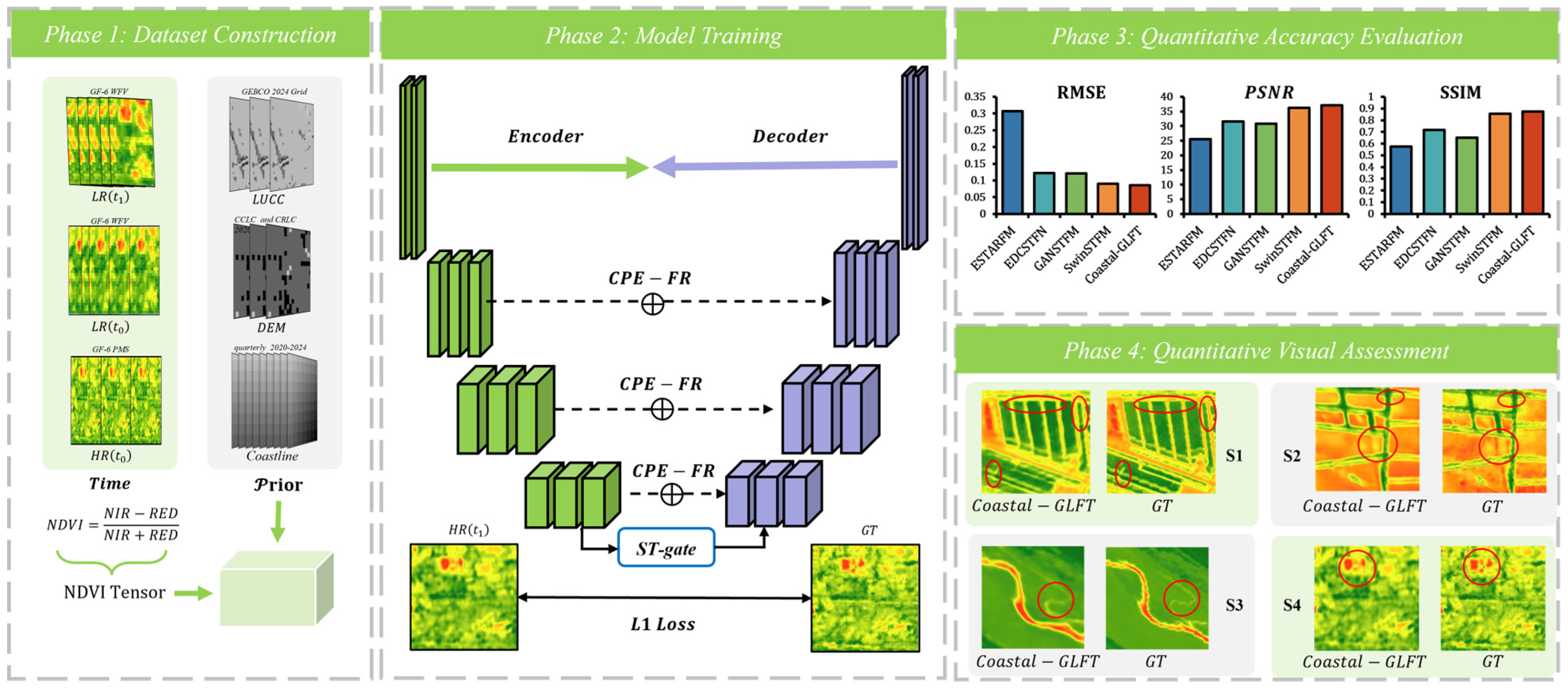
To address these challenges, a geographically constrained reconstruction framework was developed based on a hybrid fusion Transformer model that embeds geographic prior knowledge, termed the Coastal-Prior-Embedded Global–Local Fusion Transformer (Coastal-GLFT). The objective was to achieve robust reconstruction of 2 m high-resolution NDVI in complex coastal landscapes through the following workflow components:

• Geographic prior information, including digital elevation, coastline proximity, and land use/land cover, was integrated as explicit spatial constraints to guide reconstruction in accordance with underlying geospatial structure and to preserve fine boundaries in highly heterogeneous environments.
• A spatiotemporal gating mechanism was introduced to capture dynamic variations and suppress environmental interference, enabling improved separation of true land-cover change from background noise.
• A parallel global–local dual-branch architecture was developed to improve the balance between local detail and broader spatial consistency, combining detailed local information with larger-scale (global) context to preserve both fine features and overall spatial consistency.

Together, these components provide a unified multiscale framework for improving the accuracy and structural consistency of NDVI reconstruction across adjacent, sharply bounded coastal features under dynamic environmental conditions.

2. Materials and Methods

2.1. Dataset

This section describes the datasets, geographic prior information, and reconstruction framework used to generate high-resolution NDVI in complex coastal environments. The methodology first introduces the study area and construction of the multi-source image dataset, followed by the development of auxiliary geographic prior datasets representing terrain, coastline proximity, and land cover. The overall Coastal-GLFT framework is then presented, including the encoder–decoder architecture, feature extraction backbone, geographic-prior integration strategy, spatiotemporal gating mechanism, and global–local fusion module. Together, these components are designed to improve reconstruction accuracy, preserve fine coastal boundaries, and maintain larger-scale spatial consistency under dynamic environmental conditions.

2.1.1. Study Area

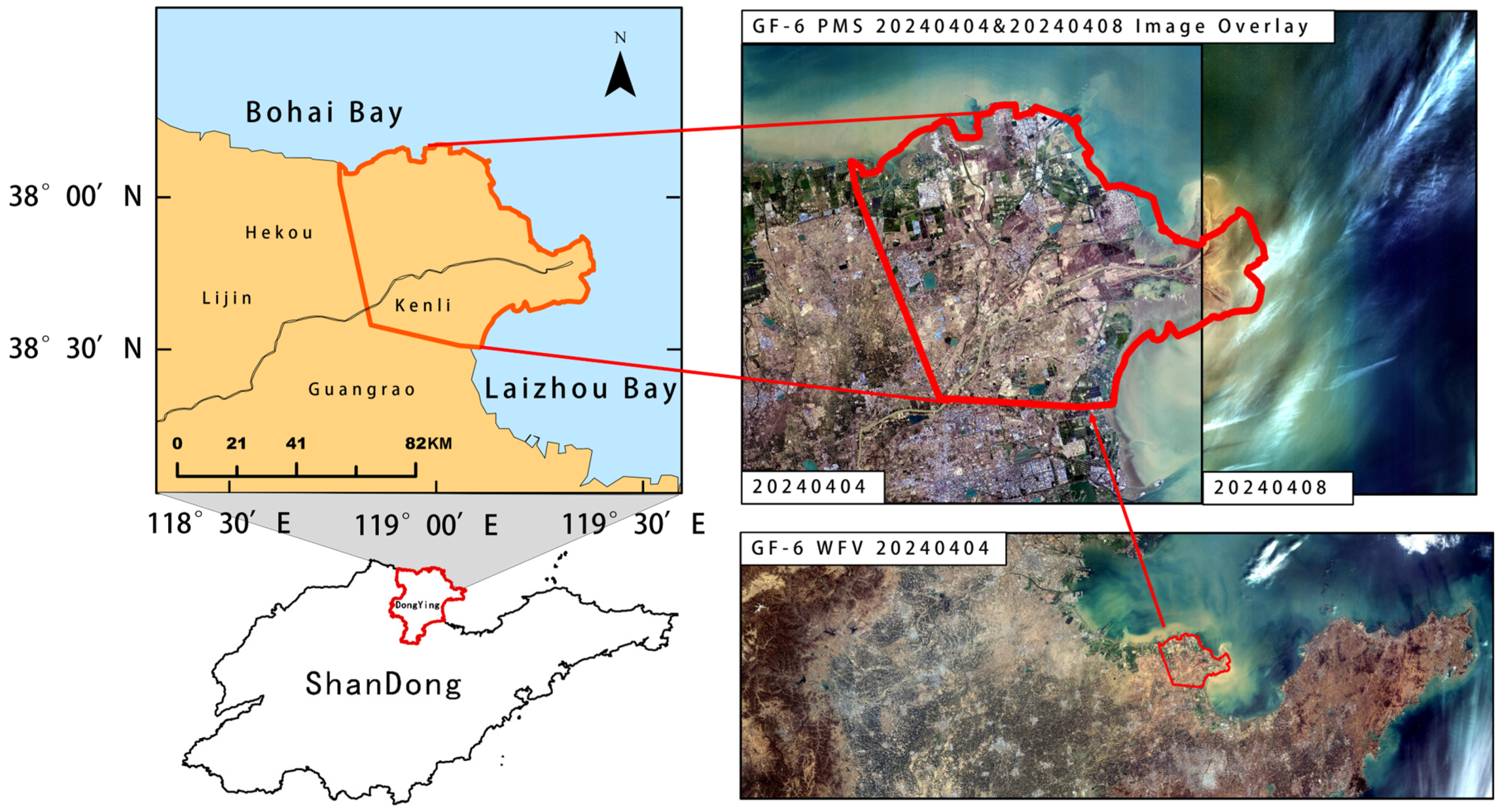
This study focuses on the Yellow River Delta, located at the interface of Bohai Bay and Laizhou Bay in China, with the Yellow River estuary and adjacent land–sea transition zone forming the core study region (Figure 1) [41]. As a representative muddy coastal system, the area is subject to strong coupled terrestrial and marine processes, including sediment deposition, tidal forcing, and shoreline migration, which drive continuous land cover evolution [42]. These processes produce a highly heterogeneous dynamic landscape characterized by intricate tidal creek networks, extensive coastal wetlands, and fragmented anthropogenic features such as reclaimed land and aquaculture ponds.

This combination of rapid environmental change and fine-scale spatial complexity presents a significant challenge for monitoring by remote sensing. Conventional single-satellite sensors typically struggle to simultaneously capture both the high-frequency temporal variability and the detailed spatial structure required to resolve these features. Consequently, the Yellow River Delta provides a suitable testbed for evaluating spatiotemporal reconstruction methods, as it requires an accurate representation of both dynamic processes and sharply defined fine-scale spatial boundaries.

This setting therefore enables rigorous assessment of the ability of the proposed framework to reconstruct high-resolution NDVI under conditions of strong heterogeneity and frequent land cover transitions from complex land–sea interactions. Building on this foundation, the following section describes the construction of the multi-source image dataset used to support model training and evaluation.

2.1.2. Construction of the Image-Pair Dataset

To effectively evaluate the reconstruction performance of the Coastal-GLFT model in complex coastal scenes, a dedicated high-resolution remote sensing spatiotemporal fusion dataset was constructed using multi-sensor imagery from the Chinese GF-6 satellite [14,16,43]. All raw data were acquired as standard Level-4 products from the China Centre for Resources Satellite Data and Application (CRESDA) and pre-processed for radiometric calibration and geometric correction.

Based on these standard products, an additional preprocessing workflow was conducted to prepare the PMS and WFV images for multi-resolution NDVI reconstruction. The images were first organized according to acquisition date and sensor type, and scenes with excessive cloud contamination or incomplete coverage of the study area were excluded. The selected PMS and WFV images were then clipped to the study area and processed for radiometric consistency and reflectance normalization to improve the comparability of multi-temporal and multi-sensor observations. Spatial consistency between PMS and WFV images was checked and adjusted based on projection information, image extent, and grid alignment. NDVI was subsequently calculated from the red and near-infrared bands. Invalid pixels and abnormal values were removed, and auxiliary geographic variables were spatially matched to the GF-6 image grid before model training and validation. This workflow ensured that the PMS, WFV, and auxiliary geographic data were spatially consistent and suitable for subsequent spatiotemporal image-pair construction.

The characteristics of the Gaofen-6 sensors (China Academy of Space Technology, Beijing, China), listed in

Table 1. Specifications of Spatiotemporal Image-Pair Data Sources.

Sensor/Payload	Panchromatic and Multispectral Sensor (PMS)	Wide-Field View Camera (WFV)
Spatial Resolution	2 m	16 m
Swath Width	90 km	800 km
Revisit Period	41 days	4 days
Spectral Band Configuration	5 conventional bands:	8 multispectral bands:
	Panchromatic (0.45–0.90 μm)	Blue, Green, Red, NIR (same as PMS)
	Blue (0.45–0.52 μm)	Coastal (0.40–0.45 μm)
	Green (0.52–0.59 μm)	Yellow (0.59–0.63 μm)
	Red (0.63–0.69 μm)	Red Edge 1 (0.69–0.73 μm)
	Near-Infrared (NIR) (0.77–0.89 μm)	Red Edge 2 (0.73–0.77 μm)
Radiometric Calibration Accuracy	Absolute accuracy: Better than 7%	Absolute accuracy: Better than 7%
	Relative accuracy: Better than 3%	Relative accuracy: Better than 3%

, underpin the design of this dataset. The Gaofen-6 platform is equipped with a panchromatic–multispectral (PMS) sensor at 2 m spatial resolution and a wide-field view (WFV) sensor at 16 m resolution. During same-day overpasses, these two sensors share highly consistent atmospheric transmission paths and sun-sensor observation geometries [16]. PMS imagery provides detailed spatial structure, while the WFV imagery offers high temporal frequency, forming a complementary dataset for spatiotemporal reconstruction. These complementary characteristics define the data selection and sampling strategy. This inherent physical consistency significantly mitigates radiometric normalization errors during multi-source fusion, making it an ideal data source for spatiotemporal reconstruction.

Images acquired between 2020 and 2025 with less than 30% cloud cover over the study area were selected. The selection strategy aimed to acquire one to two wide-field (WFV) images and one high-resolution (PMS) image per month wherever possible, resulting in a dataset comprising 49 PMS scenes and 137 WFV scenes. The specifications of the two sensors, including spatial resolution, spectral configuration, and radiometric accuracy, are summarized in Table 1.

These selected data were then organized to explicitly represent spatiotemporal relationships for model training. To ensure temporal consistency between high-resolution PMS observations and wide-field WFV observations, near-synchronous acquisitions were defined as PMS–WFV image pairs acquired within one day. In practice, most paired PMS and WFV observations were acquired within approximately one hour because the two sensors are carried by the same GF-6 satellite platform. Same-day PMS–WFV observations were preferentially selected whenever available. This temporal constraint ensured that the paired PMS and WFV images represented comparable surface conditions during image-pair construction.

To support model training, spatiotemporal image pairs were determined based on a reference–target framework. For each sample, PMS and WFV images acquired at a reference date were paired with WFV imagery at a target date, with the corresponding PMS image at the target date serving as the reconstruction ground truth. This structure enables the model to learn the mapping between high-resolution spatial detail and temporal variation across dates. The effectiveness of this mapping depends on maintaining temporal consistency between paired observations.

To ensure consistent pairing of derived relationships, near-synchronous PMS and WFV acquisitions were selected for both reference and target dates wherever possible. The resulting data reliably pair high-resolution spatial features and low-resolution temporal signals for modeling. All image pairs were spatially aligned and divided into fixed-size patches to meet neural network input requirements. This process yielded 99,867 valid paired samples for model training and evaluation. Building on this dataset, the following subsection introduces the auxiliary geographic data used to constrain the reconstruction process.

2.1.3. Construction of the Coastal-Prior-Knowledge Dataset

To address limitations of purely data-driven reconstruction, auxiliary geographic datasets were incorporated to provide physically meaningful spatial constraints on NDVI reconstruction. These geographic constraints comprised three components: digital elevation, distance to coastline, and land use/land cover, each representing important controls on coastal morphology, hydrological connectivity, and vegetation distribution. These variables were selected to represent key controls on coastal morphology and vegetation distribution, and their data sources, processing parameters, and roles in constraining coastal spatial patterns are summarized in

Table 2. Data Sources for Coastal Prior Knowledge.

Prior Factor	Data Sources and Processing Parameters	Geospatial Significance and Classification Description
DEM	Copernicus DEM 2020 Grid (30 m) [44]; processed via spatial cropping, alignment, and resampling.	Represents terrain elevation and associated hydrological connectivity, providing altitude-based constraints on the spatial distribution of vegetation and geomorphological features such as tidal flats and water systems.
Distance to Coastline	Based on quarterly shoreline variation data (2020–2024), converted into continuous gradient tensors using Euclidean distance spatial analysis.	Represents the spatial gradient of land–sea interaction, providing a topological constraint on the distribution of surface features and their proximity to the shoreline.
LUCC	Constructed via mosaicking CCLC [45] (10 m, 79.3% accuracy) and CRLC [46] (10 m, 84% accuracy) data.	Represents surface reflectance characteristics and baseline land-cover states, including 11 coastal classes: cropland, forest, shrubland, grassland, impervious surface, barren land, water bodies, herbaceous wetland, artificial wetland, mudflat, and sandy beach.

.

Digital elevation data were obtained from the Copernicus DEM 2020 Grid at 30 m resolution and processed through spatial cropping, alignment, and resampling to match the resolution and extent of the satellite imagery [40]. Elevation constrains terrain structure and hydrological connectivity, influencing the distribution of tidal flats, wetlands, and water bodies across the coastal landscape. Complementing this topographic control, proximity to the coastline represents the spatial gradient of land–sea interaction and the influence of shoreline position on land-cover distribution and evolution. Distance-to-coastline data were derived from multi-temporal shoreline vectors (2020–2024) and converted into continuous raster fields using Euclidean-distance analysis. Together, elevation and coastline proximity provide physically meaningful constraints on spatial organization within dynamic coastal environments. Land use/land cover information was incorporated as an additional constraint describing surface characteristics and expected spatial patterns of different coastal land-cover types.

Land use/land cover (LUCC) data were constructed by mosaicking two datasets: the China Coastal Land Cover (CCLC) dataset (10 m resolution, 79.3% accuracy) and the China Regional Land Cover (CRLC) dataset (10 m resolution, 84% accuracy). The combined product includes 11 coastal land-cover classes, comprising cropland, forest, shrubland, grassland, impervious surfaces, barren land, water bodies, herbaceous wetlands, artificial wetlands, mudflats, and sandy beaches. These classes provide information on expected surface characteristics, spatial organization, and spectral behavior, helping distinguish between coastal land-cover types that may exhibit similar spectral responses in remote sensing imagery. Together with elevation and coastline proximity, the LUCC data provide complementary geographic constraints during reconstruction.

All prior variables were spatially aligned with remote sensing imagery and converted into continuous raster representations before co-registration with the image patches used for model training. These prior datasets were then incorporated as additional inputs to the reconstruction framework, enabling the model to integrate geographic context during feature extraction and fusion. Although these priors provide useful spatial constraints, their effectiveness depends on the quality and temporal consistency of the underlying datasets, which may introduce uncertainty in regions undergoing rapid environmental change. This integrated multi-source dataset forms the basis of the geographically constrained reconstruction framework described in the following section.

2.2. Overall Architecture

The proposed Coastal-Prior-Embedded Global–Local Fusion Transformer (Coastal-GLFT) is designed as an end-to-end framework for reconstructing high-resolution NDVI by integrating multi-temporal satellite observations with auxiliary geographic information. The model follows a non-linear mapping paradigm, combining high-resolution spatial structure from a reference date with low-resolution temporal variation from a target date, while incorporating geographic priors to constrain the reconstruction process. This formulation enables the generation of high-resolution NDVI at the target date from multi-source inputs. This overall mapping can be formally expressed as follows:

$$\widehat{HR}\left(t_1\right)={\mathcal{M}}_{Coastal-GLFT}\left(LR\left(t_0\right),LR\left(t_1\right),HR\left(t_0\right),\mathcal{P};\mathsf{\Theta }\right)$$

(1)

where $LR\left(t_0\right)\mathrm{and}LR\left(t_1\right)$ denote the low-resolution NDVI images at the reference date and target date, respectively. $HR\left(t_0\right)$ denotes the high-resolution NDVI image at the reference date, and $\widehat{HR}\left(t_1\right)$ denotes the reconstructed high-resolution NDVI at the target date. During training, the observed $HR\left(t_1\right)$ is used as the ground truth. $\mathcal{P}$ represents the geographic prior data, including elevation, coastline proximity, and land use/land cover. 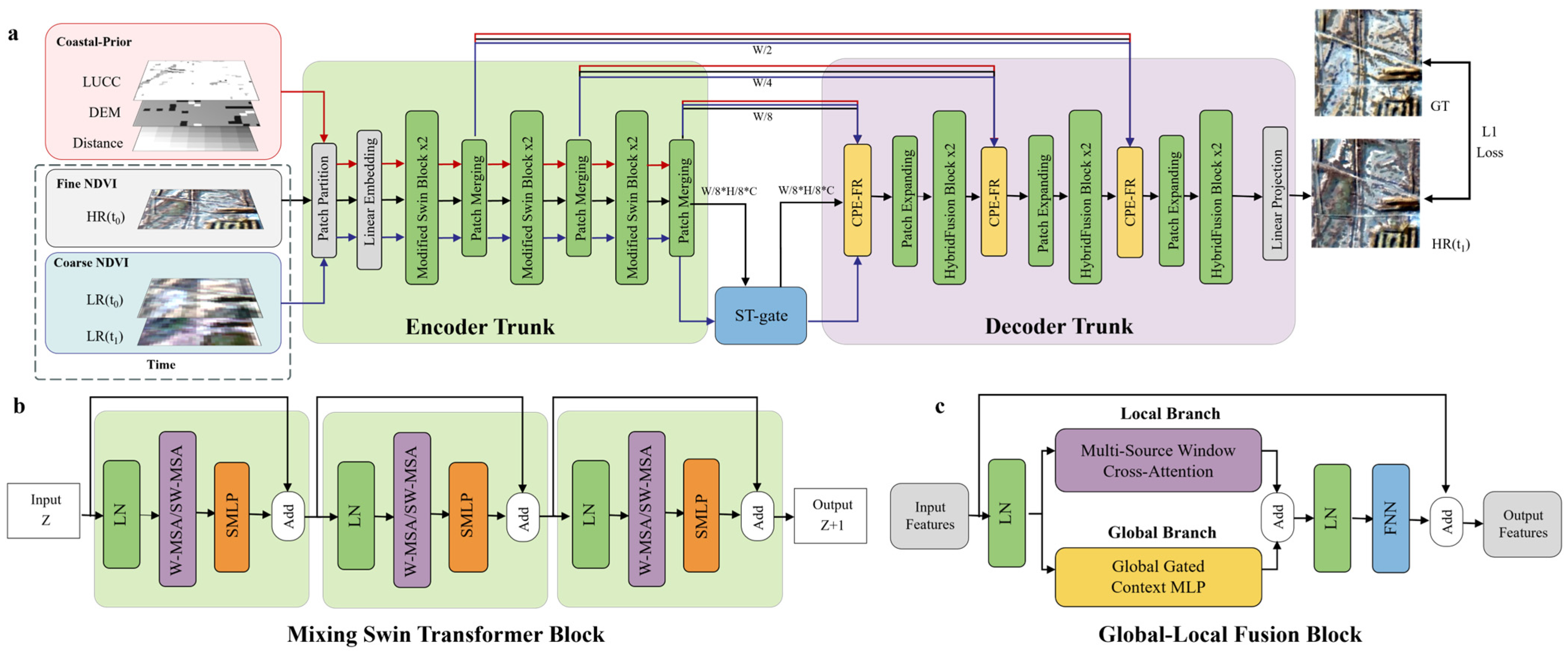$\mathsf{\Theta }$ denotes the learnable model parameters. This formulation defines the inputs and outputs of the reconstruction problem and provides the basis for the network architecture shown in Figure 2.

The architecture uses a symmetric U-shaped encoder–decoder structure built on the proposed Mixing Swin Transformer backbone (Figure 3). Mixing Swin Transformer refers to a modified Swin Transformer feature-extraction backbone in which window-based self-attention is combined with additional spatial mixing operations to improve representation of fine coastal textures and boundaries. This backbone is used to encode multi-scale features while maintaining computational efficiency, and its detailed block structure is described in Section 2.3. This backbone provides the feature-extraction structure within which the different input streams are separated and then progressively fused.

To preserve the distinct physical meanings of heterogeneous inputs, initial feature extraction is decoupled into two groups of parameter-independent branches. The first group, the multi-temporal NDVI branch, consists of a fine-resolution branch dedicated to extracting detailed spatial structures from $HR\left(t_0\right)$, and a coarse-resolution temporal branch designed to capture variation signals from the low-resolution sequence ($LR\left(t_0\right)$ and $LR\left(t_1\right)$). The second group is the Geographic-Prior branch, which uses separate encoding paths for land use/land cover, digital elevation, and distance to coastline. This separation reduces feature entanglement and allows each data source to contribute according to its physical role in the reconstruction.

The forward propagation of Coastal-GLFT consists of five main steps. First, $LR\left(t_0\right)$, $LR\left(t_1\right)$, and $HR\left(t_0\right)$ are embedded through the multi-temporal NDVI branches to extract image-derived spatial and temporal features. Second, the auxiliary geographic priors $P$ are encoded through independent prior-encoding branches to generate geographic constraint features. Third, the image features and prior features are processed through the hierarchical encoder, where patch-merging operations progressively reduce spatial resolution and increase contextual representation. At the same time, skip connections retain fine-scale NDVI features and geographic-prior information for later decoding. Fourth, at the bottleneck stage, the spatiotemporal gating mechanism selectively emphasizes meaningful temporal-change features and suppresses background variability and noise. Finally, the decoder progressively restores spatial resolution and reconstructs $\widehat{HR}\left(t_1\right)$ through Coastal-Prior-Embedded Feature Refinement modules and the Global–Local Fusion Block.

During decoding, skip-connected features from the encoder are reintroduced to recover fine spatial detail and geographic-context information that may be weakened during down-sampling. The Coastal-Prior-Embedded Feature Refinement modules integrate decoder features, skip-connected image features, and geographic-prior features to improve boundary preservation and structural consistency. The decoder further incorporates a parallel global–local fusion strategy, in which the local pathway preserves fine-scale boundary detail and the global pathway maintains broader scene-level spatial continuity across heterogeneous coastal regions. Together, these components form a multi-scale architecture for geographically constrained 2 m NDVI reconstruction in complex coastal landscapes.

2.3. Visual Backbone and Encoder–Decoder Structure

The feature extraction backbone of Coastal-GLFT is constructed using a hierarchical Swin Transformer architecture, which provides an efficient balance between computational complexity and the ability to model long-range spatial dependencies. Both the encoder and decoder adopt a symmetric pyramid structure, in which spatial resolution is progressively reduced in the encoder to capture higher-level semantic representations and subsequently restored in the decoder through successive up-sampling operations. This hierarchical design enables multi-scale representation of coastal landscapes, ranging from fine spatial textures to broader structural patterns (Figure 3a).

However, standard Swin Transformer architectures may under-represent sharp spatial gradients and fragmented fine-scale structures in highly heterogeneous coastal environments. To address this limitation, a modified backbone, termed the Mixing Swin Transformer, is introduced (Figure 3b).

The decoder stage incorporates a Global–Local Fusion Block (Figure 3c) to ensure the fidelity of the reconstructed spatial structure. A detailed technical description and the mathematical formulation of the Global–Local Fusion Block are provided in Section 2.6.

To reconstruct complex coastal landscapes accurately, the feature-extraction backbone must represent both larger-scale spatial relationships and fine-scale boundary detail. Window-based self-attention is effective for capturing broader contextual structure but can under-represent sharp spatial gradients and fragmented coastal features such as tidal creeks and aquaculture boundaries. To address this limitation, we extend the standard Swin Transformer by incorporating an additional spatial mixing pathway within the feed-forward network, enabling improved representation of high-frequency spatial variation while preserving the efficiency of window-based attention. This modification is implemented within each transformer block as a combination of attention-based and spatial mixing operations.

For the i-th Mixing Swin Transformer block, feature propagation consists of a Window Multi-head Self-Attention (W-MSA) branch and a parallel Spatial Mixing Multi-Layer Perceptron (SMLP) branch, connected through residual learning:

$$\widehat{Z^l}=\mathrm{W}\text{-}\mathrm{MSA}\left(\mathrm{SMLP}\left(Z^{l-1}\right)\right)+Z^{l-1}$$

(2)

$$Z^l=\mathrm{SMLP}\left(\mathrm{SMLP}\left(\widehat{Z^l}\right)\right)+\widehat{Z^l}$$

(3)

where $\widehat{Z^l}$ and $Z^l$ denote the input and output feature tensors of the network layer, respectively; $\mathrm{LN}$ represents Layer Normalization; and $\mathrm{W}\text{-}\mathrm{MSA}$ denotes the Window Multi-head Self-Attention mechanism. The residual connections ensure stable feature propagation and enable effective integration of attention-based and spatially mixed representations. The SMLP branch provides complementary spatial feature extraction beyond attention-based processing.

Within the SMLP module, the conventional multilayer perceptron (MLP) is extended by introducing a parallel spatial mixing pathway based on large-kernel depth-wise separable convolution. This allows the model to represent local spatial gradients and fragmented coastal textures that may not be fully captured through attention-based processing alone. The SMLP operation is defined as:

$$H_{chan}=\mathsf{\sigma }\left(X{W}_1+b_1\right)$$

(4)

$$H_{spa}={\mathrm{DWConv}}_{k\times k}\left(X\right)$$

(5)

$$X_{out}=\left(H_{chan}+H_{spa}\right)W_2+b_2$$

(6)

where $H_{chan}$ denotes the channel-mixed features and $H_{spa}$ denotes the spatial-mixed features; $W_1$, $b_1$ and $W_2$, $b_2$ represent the weight matrices and bias terms of the two fully connected linear transformations, respectively; and $\mathsf{\sigma }\left(\cdot \right)$ represents the Gaussian Error Linear Unit activation function (GELU). The core operation, ${\mathrm{DW} \mathrm{Conv}}_{k\times k}\left(X\right)$, represents the depthwise separable convolution with a kernel size of $k\times k$, which is introduced in this study to efficiently capture high-frequency spatial gradients. This combined attention–convolution mechanism improves representation of complex coastal boundaries while maintaining computational efficiency. These feature representations are then aggregated across scales within the encoder–decoder structure.

Within the encoder, spatial resolution is progressively reduced through patch-merging layers, enabling the network to represent increasingly broader spatial context and large-scale structural relationships. In contrast, the decoder restores spatial resolution using corresponding patch-expanding layers, reconstructing high-resolution feature maps from the encoded representations. The symmetric encoder–decoder design maintains consistency between the down-sampling and up-sampling processes, helping preserve spatial structure and minimize distortion during feature compression and reconstruction. Skip connections further link corresponding encoder and decoder stages, allowing fine-scale spatial detail and intermediate feature representations to bypass the compressed latent representation and be reintroduced directly during decoding. This combination of multi-scale encoding, symmetric reconstruction, and direct feature transfer enables the model to preserve both larger-scale spatial organization and fine coastal boundary structure throughout the reconstruction process.

In the decoding stage, feature fusion is achieved through a global–local hybrid mechanism (Figure 3c), which combines detailed local information with larger-scale (global) context to preserve both fine spatial features and overall structural consistency. The local pathway captures high-frequency texture information through spatially focused feature interactions, while the global pathway represents broader spatial relationships across the entire scene. The integration of these pathways enables the model to balance boundary sharpness with large-scale coherence in reconstructed NDVI fields. The integration of geographic priors within this framework is described in the following subsection.

The computational workflow of the visual backbone is as follows. The embedded input feature $F_0$ is first partitioned into local windows and processed by window-based self-attention to capture short-range spatial dependencies. The spatial mixing operation is then applied to enhance the representation of local gradients and boundary textures. After each encoder stage, patch-merging layers reduce the spatial resolution and increase the channel dimension, enabling the model to represent broader spatial context. During decoding, patch-expanding layers progressively restore the spatial resolution, while skip connections transfer fine-scale features from the corresponding encoder stages. This process allows the backbone to jointly preserve local coastal textures and larger-scale spatial organization.

2.4. Coastal-Prior Embedding and Feature Refinement

Coastal evolution is governed by well-defined physical processes and spatial constraints, including elevation, hydrological connectivity, and proximity to the shoreline. In conventional data-driven reconstruction models, these constraints are not explicitly represented, which can result in outputs that are inconsistent with the underlying geospatial structure, particularly in highly heterogeneous regions. To address this limitation, Coastal-GLFT incorporates a dedicated coastal-prior branch to encode auxiliary geographic information and guide reconstruction. This branch enables the model to incorporate spatial constraints directly within the feature representation.

The Coastal-Prior Branch processes digital elevation, distance-to-coastline, and land use/land cover data through independent encoding pathways, ensuring that each prior source contributes distinct information without interference. These inputs are transformed into feature representations using multi-scale convolutional operators, allowing spatial constraints to be captured at multiple resolutions. The resulting prior features are aligned with the corresponding NDVI feature maps and propagated through the network alongside the multi-temporal inputs. These encoded prior features are subsequently integrated with the main feature stream during decoding.

Specifically, DEM, distance-to-coastline, and LUCC are first processed by separate prior-encoding branches to generate multi-scale prior features. These prior features are spatially aligned with the NDVI feature maps at the corresponding encoder–decoder scale. At each decoder stage, the upsampled decoder feature, the skip-connected image feature, and the corresponding geographic-prior feature are concatenated and refined by the CPE-FR module. In this way, the prior information is introduced as scale-aware spatial constraints rather than directly replacing image-derived features.

Direct fusion of heterogeneous features from multiple sources can introduce redundancy and scale mismatch, particularly when combining NDVI features with auxiliary geographic data. To address this, a Coastal-Prior-Embedded Feature Refinement (CPE-FR) module is introduced to regulate the integration of prior information. This module applies linear transformations and non-linear activation functions to align feature distributions and selectively incorporate relevant prior signals. The feature refinement process is defined as:

$$F_{in}=\left[F_{dec},F_{skip},F_{prior}\right]$$

(7)

$$F_{mid}=\sigma \left(W_1\cdot F_{in}+b_1\right)$$

(8)

$$F_{refined}=W_2\cdot F_{mid}+b_2$$

(9)

where $F_{dec}$ denotes the upsampled features, $F_{skip}$ represents the skip-connection features from the corresponding encoder scale, $F_{prior}$ signifies the geographic prior features encoded by the prior branch, and $\left[ \cdot \right]$ denotes the concatenation operation along the channel dimension. $W_1,b_1$ and $W_2,b_2$ represent the weight matrices and bias terms of the two linear transformations within CPE-FR, respectively; and $\sigma$ is the GELU non-linear activation function. $F_{in}$ represents the initial set of heterogeneous features received by the module, $F_{mid}$ represents the fused structure after preliminary filtering and non-linear compression, and $F_{refined}$ is the final output of the CPE-FR module that combines NDVI information and geographic constraints. This mechanism enables adaptive integration of prior information across scales.

Through this refinement process, geographic priors act as conditional spatial constraints that guide reconstruction without overwhelming the NDVI feature representation. The model can therefore selectively emphasize prior information where it improves boundary delineation and spatial consistency, while reducing its influence in regions where auxiliary datasets may be uncertain or temporally outdated. This adaptive weighting is particularly important in dynamic coastal environments, where rapid land-cover change can produce mismatches between prior datasets and current surface conditions. As a result, the framework can incorporate geographic guidance while remaining responsive to genuine environmental variability.

Together, the coastal-prior branch and CPE-FR module provide a controlled and scale-aware mechanism for incorporating geographic information into the reconstruction framework. This improves preservation of fine coastal boundaries and reduces structural inconsistencies that commonly arise in purely data-driven approaches. The modeling of temporal variation and suppression of background noise within this framework is described in the following subsection.

2.5. Differential-Driven Spatiotemporal Gating

Coastal regions are frequently disrupted by severe cloud cover and highly dynamic atmospheric water vapor, which often introduces substantial non-target variation noise into remote sensing imagery. Conventional feature-stacking fusion approaches often treat all temporal differences as signal, making it difficult to distinguish genuine land-cover change from background noise. To address this limitation, Coastal-GLFT incorporates a differential-driven spatiotemporal gating mechanism (ST-gate) to explicitly model temporal variation and regulate feature propagation. This mechanism enables the model to emphasize meaningful change while suppressing irrelevant variation.

The ST-gate operates at the bottleneck of the encoder–decoder architecture, where features from different time steps are jointly represented. It compares the difference between low-resolution feature representations at the reference and target dates to identify regions of significant temporal variation. These different features are then transformed into a gating mask through a learnable projection and non-linear activation, which is used to modulate the feature map. The gating process is defined as:

$$M=\mathsf{\sigma }\left(\mathsf{\varphi }\left(\mathcal{D}\left(F_1,F_0\right)\right)\right)$$

(10)

where $\mathcal{D}$ denotes the feature difference operator; $\varphi$ is the feature projection function; $F_0$ and $F_1$ denote feature representations at the reference time $t_0$ and target time $t_1$, respectively, extracted from the low-resolution temporal branch prior to gating; and $\sigma$ is the Sigmoid activation function. Ultimately, the gated features are obtained by performing element-wise weighting on the original feature stream using the mask $M$. This formulation allows the model to selectively weight features based on temporal variation.

Through this mechanism, regions exhibiting significant temporal change are assigned higher weights, while relatively stable or noise-affected regions are suppressed. This reduces the influence of atmospheric artifacts and transient surface conditions that do not correspond to actual land-cover dynamics. At the same time, the gating process remains adaptive, allowing the model to respond to varying levels of temporal variability across different spatial contexts. This selective weighting improves the robustness of feature representations passed to the decoder.

By integrating the ST-gate within the bottleneck, the model applies temporal filtering at a stage where both local detail and global context are represented, enabling effective discrimination between signal and noise across scales. This contributes to a more stable reconstruction of NDVI under complex environmental conditions, particularly in coastal regions where temporal variability is high. The integration of spatial detail and global context in the decoding stage is described in the following subsection.

2.6. Global–Local Fusion Block

Accurate reconstruction of NDVI in coastal landscapes requires simultaneous preservation of fine-scale spatial detail and larger-scale structural consistency. Conventional approaches often favor one at the expense of the other, leading either to over-smoothed boundaries or to spatial discontinuities. Recent studies indicate that the window partitioning in self-attention mechanisms restricts the effective receptive field, causing window-based Transformers to prioritize local feature extraction at the expense of global modeling capabilities [40]. To overcome this limitation in capturing multi-scale coastal dependencies, Coastal-GLFT incorporates a Global–Local Fusion Block within the decoder (Figure 3c). This design enables the model to balance detailed texture reconstruction with overall spatial coherence. Although attention mechanisms are commonly associated with global dependency modeling, their actual spatial role depends on the spatial extent over which feature interactions are computed. In the proposed Global–Local Fusion Block, the window-based attention branch restricts feature interactions to neighboring regions within local windows. Therefore, this branch functions as a local structural modeling branch rather than a fully global attention module. This design is consistent with the physical characteristics of coastal landscapes where abrupt NDVI gradients and strong local heterogeneity are frequently observed. Restricting feature interactions to local windows therefore helps preserve fine boundaries while reducing inappropriate mixing between spectrally similar but physically distinct surfaces. In contrast, the global branch provides broader contextual information, such as land–sea gradients and regional vegetation patterns, thereby complementing the local branch and jointly maintaining scene-level spatial consistency.

The global–local fusion block operates on feature maps propagated from the decoder and corresponding skip connections, combining information from local and larger-scale contexts through parallel processing pathways. The local pathway focuses on high-resolution spatial detail, using cross-attention mechanisms to selectively integrate fine-scale features from multi-source inputs. This allows the model to preserve sharp boundaries and capture detailed textures associated with heterogeneous coastal land-cover types. In contrast, the global pathway captures broader spatial relationships across the scene.

The global pathway processes the same input features using a gated multilayer perceptron, which aggregates information over larger spatial regions and represents macroscopic spatial structure. This pathway enables the model to maintain consistency across land–water transitions and prevent fragmentation of spatial patterns during reconstruction. The outputs of the local and global pathways are then adaptively integrated to produce a unified representation. This fusion ensures that both local detail and global structure are retained in the reconstructed output. The local branch reconstructs fine spatial detail by selectively transferring structure from the reference image, while the global branch preserves larger-scale spatial organization.

For clarity, the adaptive balance between the local and global branches can be expressed in a simplified form as:

$$F_{fused}=\alpha \cdot {\mathit{Branch}}_{local}+\left(1-\alpha \right)\cdot {\mathit{Branch}}_{global}$$

(11)

where $F_{\mathrm{f}\mathrm{u}\mathrm{s}\mathrm{e}\mathrm{d}}$ denotes the fused feature representation, $F_{\mathrm{l}\mathrm{o}\mathrm{c}\mathrm{a}\mathrm{l}}$ and $F_{\mathrm{g}\mathrm{l}\mathrm{o}\mathrm{b}\mathrm{a}\mathrm{l}}$ denote the representations from the local and global pathways, respectively, and $\alpha$ denotes an adaptive balancing coefficient that controls the relative contribution of local detail and broader spatial context. This parallel interaction mechanism enables Coastal-GLFT to overcome the edge-smoothing phenomenon common in traditional Transformers, which stems from an over-reliance on global semantics. As a result, while preserving macroscopic semantics, the model maximally restores the fine structures of complex coastal surface spatial textures. The final fused feature $F_{fused}$ integrates complementary spatial information across scales. This fused representation is then used to generate the final high-resolution NDVI output.

For the local branch, component mechanisms contributing to the local branch were formulated as:

$$Q=F_{refined}{W}_Q$$

(12)

$$K=F_{enc}^{t_0}{W}_K$$

(13)

$$V=F_{enc}^{t_0}{W}_V$$

(14)

$${\mathit{Branch}}_{local}=\mathit{Softmax}\left({\displaystyle \frac{Q{K}^T}{\sqrt{d}}}+B\right)V$$

(15)

where $Q,K,V$ are the query, key, and value vectors, respectively. $F_{refined}$ is the final output of the CPE-FR module that combines NDVI information and geographic constraints, and $F_{enc}^{t_0}$ denotes the encoded feature representation extracted from the reference date $t_0$. The query vector $Q$ carries the semantic positional information of the target date $t_1$, while $K$ and $V$ provide the spatial structure of the reference date $t_0$. $W_Q$, $W_{\mathrm{K}}$, and $W_{\mathrm{V}}$ are learnable linear projection matrices used to generate the query, key, and value matrices, respectively. $W_Q$ projects decoder features into the query space, while $W_{\mathrm{K}}$ and $W_{\mathrm{V}}$ project reference high-resolution features into the key and value spaces. This design allows the local attention branch to match decoder features with fine-scale reference structures and selectively aggregate local spatial details. $\mathit{Softmax}$ is the normalized exponential activation function, $B$ is the relative position bias, and $d$ represents the channel dimension of the $Q$ and $K$ vectors during the dot-product computation. For the global branch, the formulation was:

$$G=\sigma \left(\mathit{FC}\left(\mathit{GlobalAvgPool}\left(F_{refined}\right)\right)\right)$$

(16)

$${\mathit{Branch}}_{global}=G\odot \mathit{MLP}\left(F_{refined}\right)$$

(17)

where $\mathit{GlobalAvgPool}$ is global average pooling, $G$ is the gating weight (a global gating mask generated through a fully connected layer (FC) and a Sigmoid activation function), and $\odot$ represents element-wise multiplication.

By combining local detail with larger-scale spatial context, the global–local fusion block reduces boundary blurring while maintaining continuity of spatial patterns across the scene. This is particularly important in coastal landscapes, where adjacent land-cover types often exhibit sharp transitions and complex spatial arrangements. The parallel design also allows the model to adaptively weight contributions from each pathway depending on local spatial complexity. Together with the preceding spatiotemporal gating mechanism, this fusion strategy supports robust reconstruction under heterogeneous and dynamic conditions.

3. Results

This section evaluates the performance of the proposed geographically constrained spatiotemporal fusion framework for generating 2 m NDVI in complex coastal landscapes. The evaluation is designed to assess whether the integration of multi-source data and geographic priors improves reconstruction accuracy, spatial consistency, and robustness to environmental variability through comprehensive comparisons with representative baseline methods. To achieve this, we first describe the experimental configuration, including data partitioning, model training, and parameter settings. This is followed by quantitative evaluation against established methods using standard image reconstruction metrics, and qualitative assessment across representative coastal land-cover types to examine boundary preservation and spatial coherence. Finally, the results are analyzed to determine the contribution of individual model components and to assess the robustness of the approach under heterogeneous and dynamic coastal conditions. The experimental setup underlying these evaluations is described in the following subsections.

3.1. Experimental Setup

This experimental setup was designed to evaluate the spatiotemporal fusion performance of models based on the Coastal-GF6-STF dataset for the Yellow River Delta. This evaluation provides a consistent basis for comparing the reconstruction capabilities of different models. The dataset was randomly divided into a training set and a testing set with a ratio of 9:1 respectively. Each sample comprises a spatiotemporal quadruple image pair $\{LR\left(t_1\right),LR\left(t_0\right),HR\left(t_0\right),HR\left(t_1\right)\}$, where $LR$ and $HR$ denote low-resolution and high-resolution NDVI images at times $t_0$ (reference) and $t_1$ (target), respectively. Spatial dimensions were $256\times 256$ pixels for fine-resolution images and $32\times 32$ pixels for coarse-resolution images.

Coastal-GLFT was implemented using the PyTorch (1.13.1) framework. For network configurations, we adopted settings from Swin-Tiny as follows [37]:

• The number of Mixing Swin Transformer blocks in the encoder stage was set to [2, 2, 6, 2], respectively.
• Within the feature extraction backbone, the base-channel number (C) was set to 96, and the corresponding numbers of attention heads for the Multi-head Attention mechanism were configured as [3, 6, 12, 24].
• Inside each Mixing Swin Transformer block, the window size for local self-attention was set to $8\times 8$.
• Concurrently, the kernel size of the parallel large-kernel depth-wise separable convolution in the SMLP module was set to $7\times 7$ to efficiently capture high-frequency spatial gradients in coastal zones.
• The adaptive fusion parameter $\mathsf{\alpha }$ in the Global–Local Fusion Block was initialized as a learnable tensor.

These architectural parameters define the model configuration used in all experiments. To ensure a comprehensive comparative evaluation of our Coastal-GLFT, four spatiotemporal fusion models representing different paradigms (physics-driven, CNN-based, GAN-based, and Transformer-based) were selected as baselines. All baseline models were trained from scratch using identical training strategies to ensure comparability. This consistent training protocol provides the basis for fair performance comparison.

For learning-based models, the same training samples, input patch configuration, batch size, optimizer setting, learning rate, loss function, number of training iterations, and evaluation metrics were used wherever applicable. Specifically, the batch size was set to 16. The total number of training iterations was set to 300,000. All models utilized the AdamW optimizer (${\mathsf{\beta }}_1=0.9,{\mathsf{\beta }}_2=0.999$, weight decay = $1\times 10^{-4}$) for parameter updating, with an initial learning rate set to $1\times 10^{-4}$. During optimization, all models were trained using the L1 loss function. Training and evaluation were conducted on a workstation equipped with an NVIDIA GeForce RTX 4090 GPU (24 GB) and an Intel Core i9-14900K CPU. These settings ensure consistent optimization and computational conditions across all experiments.

3.2. Evaluation Metrics

Model performance was evaluated from three complementary quantitative metrics: Root Mean Square Error (RMSE), Peak Signal-to-Noise Ratio (PSNR), and Structural Similarity Index Measure (SSIM). These metrics collectively assess reconstruction accuracy across pixel-level error, signal fidelity, and structural similarity. Together, they provide a consistent basis for comparing model performance across different aspects of reconstruction quality.

RMSE: RMSE measures the absolute numerical difference between the predicted image and the ground-truth image at the pixel level. This measure determines the absolute accuracy of NDVI values for subsequent ecological analyses, such as biomass estimation and vegetation succession monitoring. Due to the squaring of errors, RMSE is highly sensitive to large deviations (i.e., outlier errors), making it effective for examining the prediction accuracy of models in highly dynamic regions. Its mathematical definition is:

$$\mathrm{RMSE}=\sqrt{{\displaystyle \frac{1}{N}}\sum _{i=1}^N{\left(\widehat{y_i}-y_i\right)}^2}$$

(18)

where $N$ is the total number of pixels in the image, and $\widehat{y_i}$ and $y_i$ denote the predicted NDVI value at the target date and the actual observed NDVI ground-truth, respectively.

PSNR: PSNR is used to evaluate the fidelity of reconstructed imagery by quantifying the ratio between signal and reconstruction error. In spatiotemporal fusion, reconstruction involves combining information from multiple sources, which may introduce artifacts due to temporal misalignment or sensor differences. PSNR provides a global measure of how effectively the model preserves signal content while suppressing noise. Higher PSNR values indicate lower distortion in the reconstructed image. It is defined as:

$$\mathrm{PSNR}=10\cdot {\log }_{10}\left({\displaystyle \frac{MA{X}^2}{\mathrm{MSE}}}\right)$$

(19)

where $MAX$ represents the maximum possible pixel value of the image (typically 1 for normalized NDVI), and $MSE$ is the Mean Squared Error. This scaled-maximum metric reflects the overall signal fidelity of the reconstruction.

SSIM: SSIM evaluates structural similarity between the predicted and reference images by comparing luminance, contrast, and structural information. Coastal landscapes are spatially heterogeneous, with fine-scale features such as tidal channels and land–water boundaries that may not be adequately assessed using pixel-wise error metrics alone. SSIM provides a complementary perspective by quantifying how well spatial patterns and textures are preserved. Higher SSIM values indicate greater structural similarity between reconstructed and ground-truth images. Its formulation is:

$$\mathrm{SSIM}={\displaystyle \frac{\left(2{\mu }_{\widehat{y}}{\mu }_y+C_1\right)\left(2{\sigma }_{\widehat{y}y}+C_2\right)}{\left({\mu }_{\widehat{y}}^2+{\mu }_y^2+C_1\right)\left({\sigma }_{\widehat{y}}^2+{\sigma }_y^2+C_2\right)}}$$

(20)

where $\mu$ represent local means, and $\sigma$ represent variances or covariances. $C_1$ and $C_2$ are very small constants introduced to prevent the denominator from becoming zero. This metric captures the preservation of spatial structure and texture in the reconstructed imagery.

3.3. Quantitative Performance Validation

This subsection evaluates the quantitative performance of the proposed method relative to representative spatiotemporal fusion approaches. The objective is to assess whether the geographically constrained reconstruction framework improves numerical accuracy, signal fidelity, and structural consistency, as measured by the metrics defined in Section 3.2. To achieve this, Coastal-GLFT was compared with four baseline models spanning different methodological paradigms: the Enhanced Spatial and Temporal Adaptive Reflectance Fusion Model (ESTARFM), a physics-driven method; the Enhanced Deep Convolutional Spatiotemporal Fusion Network (EDCSTFN), a convolutional neural network (CNN)-based model; the Generative Adversarial Network-based Spatiotemporal Fusion Model (GANSTFM); and the Swin Transformer-based Spatiotemporal Fusion Model (SwinSTFM).

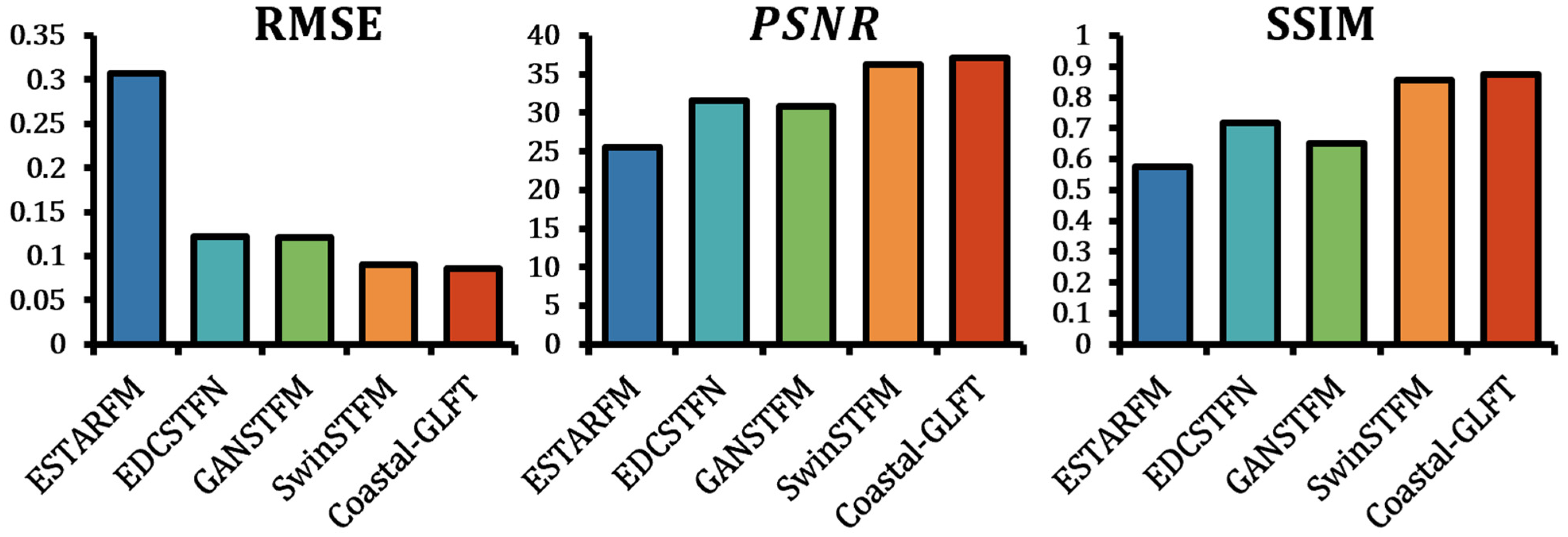
The results are summarized in

Table 3. Quantitative Evaluation Results of Different Models. (Note: The bold row represents the proposed full model, Coastal-GLFT, and its bold values indicate the best performance among all compared methods).

Model	Category	RMSE	PSNR	SSIM
ESTARFM	Physics-driven	0.3068	25.51	0.5768
EDCSTFN	CNN-based	0.1218	31.60	0.7180
GANSTFM	GAN-based	0.1206	30.85	0.6522
SwinSTFM	Transformer-based	0.0896	36.19	0.8551
Coastal-GLFT	Transformer-based	0.0855	37.09	0.8742

and further illustrated in Figure 4. These comparisons provide a consistent basis for assessing model performance across diverse reconstruction approaches.

When applied to complex coastal landscapes, both physics-based and deep learning-based models exhibit performance limitations. The physics-driven ESTARFM shows the largest reconstruction error (RMSE = 0.3068) and lowest structural similarity (SSIM = 0.5768), reflecting its reliance on linear weighting assumptions that are less suited to highly heterogeneous environments. The CNN-based EDCSTFN and GAN-based GANSTFM improve pixel-level accuracy (RMSE ≈ 0.12), but their structural similarity remains lower (SSIM ≤ 0.7180), indicating reduced ability to preserve spatial patterns. GANSTFM exhibits lower PSNR (30.85 dB), consistent with the presence of reconstruction artifacts. These results indicate that conventional approaches struggle to balance numerical accuracy and structural consistency in dynamic coastal regions.

The Transformer-based SwinSTFM provides a substantial improvement over earlier methods, achieving RMSE = 0.0896, PSNR = 36.19 dB, and SSIM = 0.8551. This reflects the advantage of attention-based architectures in capturing long-range spatial dependencies. However, its performance remains limited when representing both large-scale spatial structure and fine-scale boundary detail simultaneously, consistent with the constraints imposed by window-based attention mechanisms. This provides a relevant benchmark for evaluating the proposed method.

Compared with all baseline models, Coastal-GLFT achieves the best performance across all evaluation metrics, with RMSE = 0.0855, PSNR = 37.09 dB, and SSIM = 0.8742. Relative to the strongest baseline (SwinSTFM), this corresponds to a reduction in RMSE of approximately 4.6%, an increase in PSNR of approximately 2.5%, and an increase in SSIM of approximately 2.2%. These improvements indicate consistent gains in pixel-level accuracy, signal fidelity, and structural similarity. These performance differences reflect the combined effect of the architectural components introduced in Section 2.

The improved performance of Coastal-GLFT reflects the incorporation of geographic prior spatial constraints that improve boundary delineation in heterogeneous regions. The spatiotemporal gating mechanism reduces the influence of non-target temporal variation, contributing to improved numerical stability. In addition, the global–local fusion structure enables the model to retain both fine spatial detail and larger-scale spatial coherence. Together, these elements contribute to improved reconstruction performance under complex coastal conditions, as further examined through qualitative analysis in the following subsection.

3.4. Qualitative Validation

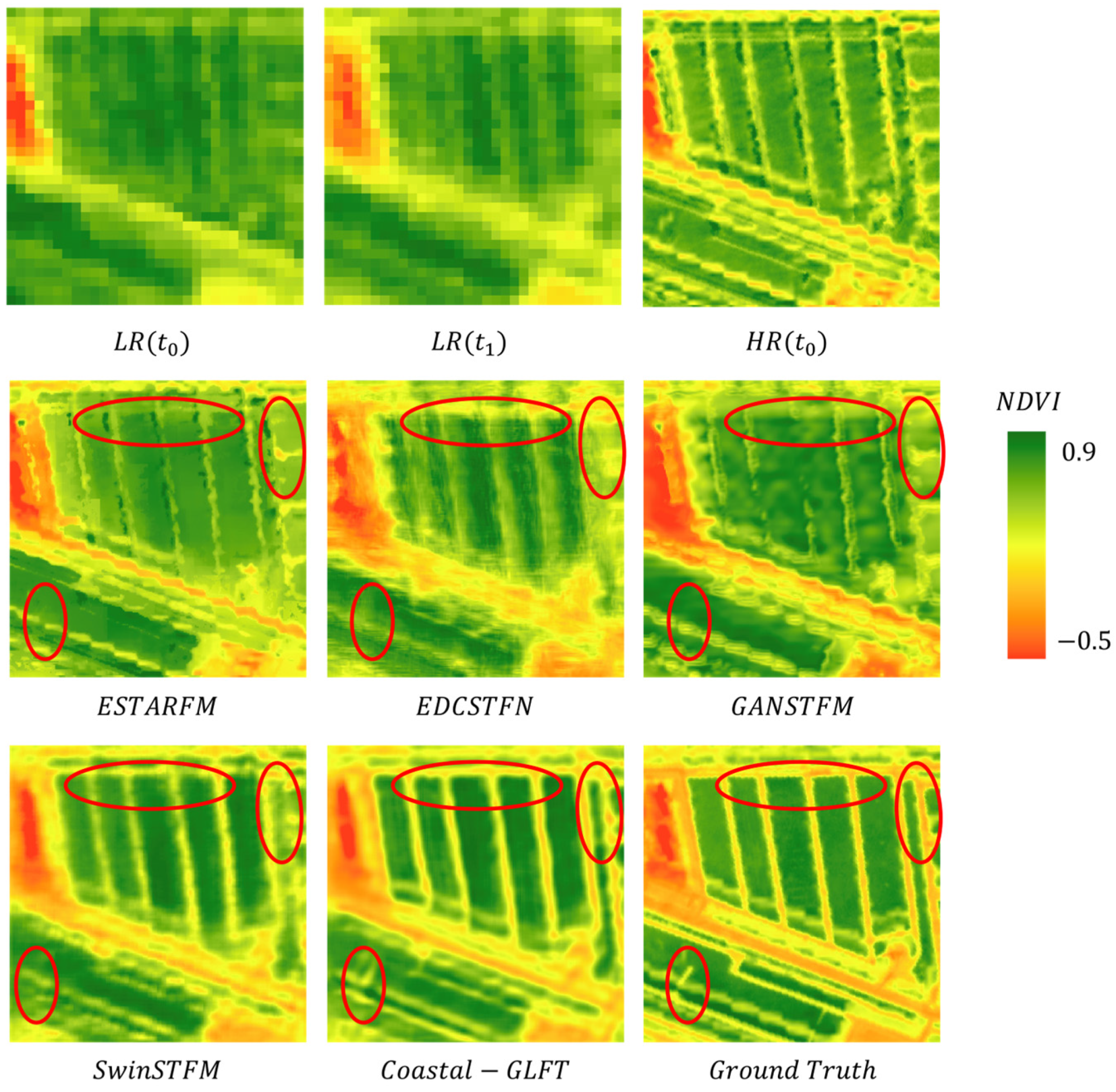
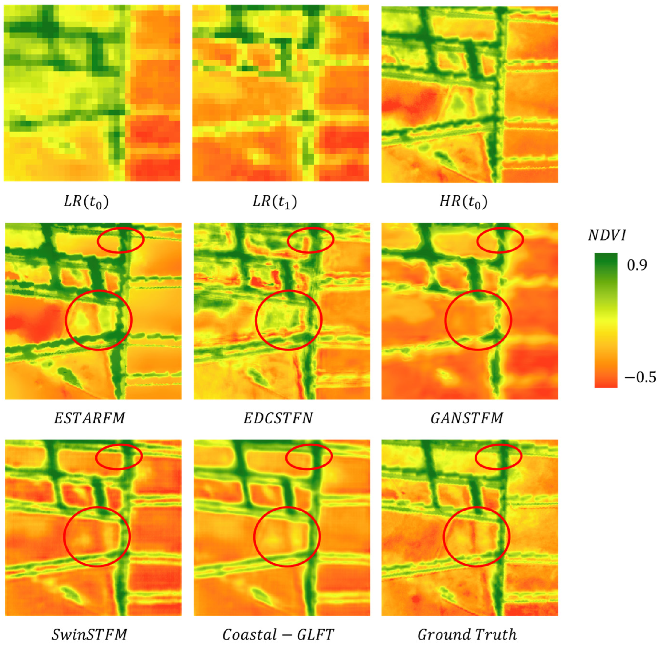
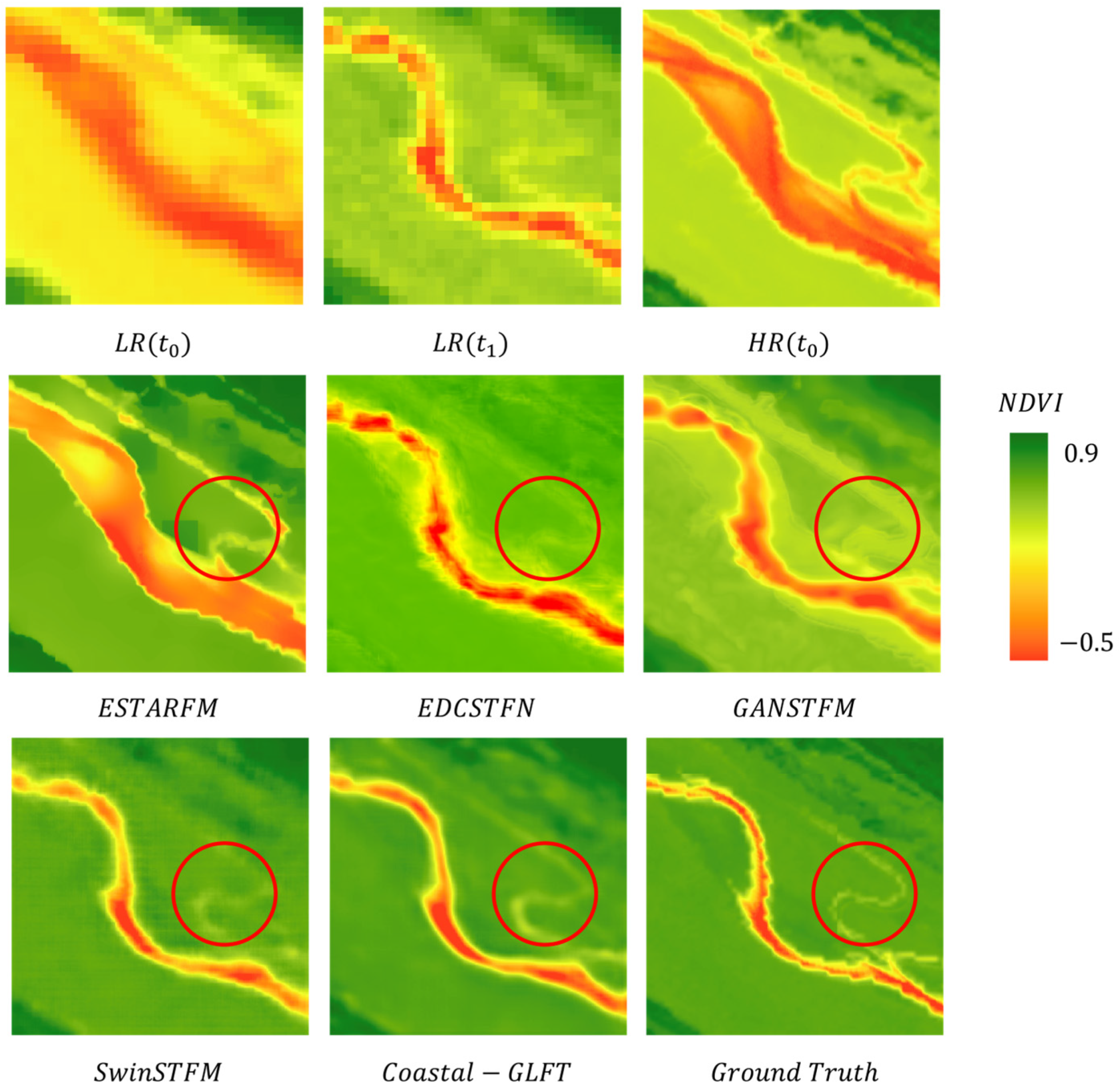
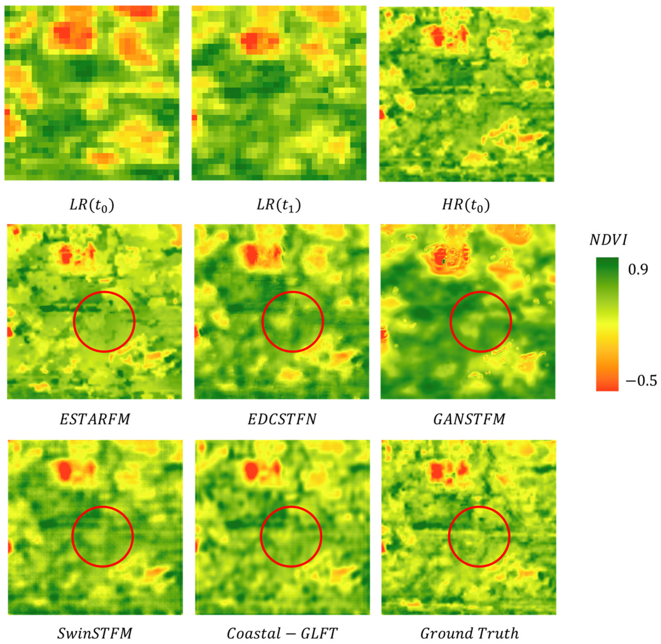
This subsection evaluates the qualitative performance of the proposed method across representative coastal land-cover types. The objective was to assess whether the improvements observed in quantitative metrics were reflected in the visual reconstruction of spatial detail, boundary definition, and structural continuity. Four characteristic scenarios were selected for validation: croplands, aquaculture ponds, tidal creeks, and natural wetlands (salt marshes).

These four scenarios were selected to represent typical coastal landscape conditions and reconstruction challenges in the Yellow River Delta. Scenario A represents cropland areas with regular field boundaries and relatively homogeneous vegetation signals. Scenario B represents aquaculture ponds, which are characterized by artificial grid-like structures, sharp land–water boundaries, and strong local contrast. Scenario C represents tidal-creek systems, where meandering channel networks and narrow tributaries require the model to preserve non-linear spatial connectivity. Scenario D represents natural wetlands and salt marshes, which are characterized by fragmented vegetation patches, strong spatial heterogeneity, and temporal variability. Together, these scenarios provide a comprehensive visual assessment of boundary preservation, structural continuity, and reconstruction stability in heterogeneous coastal environments.

(1) Croplands and Artificial Wetlands (Aquaculture Ponds)

Scenarios A (croplands) in Figure 5 and B (aquaculture ponds) in Figure 6 are characterized by regular, grid-like spatial patterns with sharp boundaries and relatively uniform internal NDVI values. These features provide a stringent test of a model’s ability to preserve geometric structure and boundary clarity. Visual comparisons (Figure 6 and Figure 7) show that the grid structures reconstructed by ESTARFM and EDCSTFN exhibit noticeable smoothing and boundary blurring, consistent with their lower SSIM values reported in Table 3. GANSTFM introduces visible artifacts in some regions, in line with its lower PSNR. In contrast, both SwinSTFM and Coastal-GLFT produce improved representations of local detail, reflecting the advantage of attention-based architectures. However, SwinSTFM still shows slight smoothing and loss of fine structure.

Coastal-GLFT exhibited the clearest grid patterns and most distinct boundary delineation among all models. Fine-scale spatial detail was preserved while maintaining overall structural consistency. These results indicate that the global–local fusion mechanism effectively balances local texture representation with broader spatial context, while the incorporation of geographic priors provides additional spatial guidance. These characteristics support improved reconstruction of structured landscapes with well-defined boundaries.

(2) Tidal Creeks

Scenario C (tidal creeks) is characterized by meandering and continuous channel networks with smooth boundaries and relatively low NDVI values. This scenario tests the ability of models to represent non-linear structures and maintain connectivity. As shown in Figure 7, ESTARFM exhibits large prediction deviations, consistent with its higher RMSE values in Table 3. Other baseline models display varying degrees of discontinuity and irregular boundary artifacts, and most fail to capture fine tributary channels.

In contrast, Coastal-GLFT reconstructs continuous and smooth channel networks while preserving fine-scale tributary structures. Boundary transitions are more consistent and less affected by artifacts compared with other models. These results indicate improved representation of complex spatial structures and reduced distortion in regions with strong geometric variability. The incorporation of geographic information, including elevation and distance to coastline, contributes to more consistent reconstruction of connected features. This demonstrates improved handling of non-linear spatial patterns in coastal environments.

(3) Natural Wetlands (Salt Marshes)

Scenario D (Figure 8) shows irregular, spatially fragmented patches of high-NDVI salt marsh vegetation. This scenario is characterized by strong spatial variability and temporal change between reference and target dates, providing a test of both structural preservation and temporal consistency. Baseline models such as ESTARFM and EDCSTFN exhibit loss of small-scale features and merging of distinct patches, while GANSTFM produces noticeable structural distortions, consistent with its lower PSNR.

Both SwinSTFM and Coastal-GLFT improve reconstruction quality in this scenario, preserving the general distribution of salt marsh patches. However, Coastal-GLFT provides more consistent representation of patch boundaries and spatial variability, with fewer artifacts and reduced distortion. These results suggest improved integration of temporal variation and spatial structure, particularly in regions with heterogeneous and evolving land cover. This supports the robustness of the proposed method under complex and dynamic conditions.

3.5. Ablation Study

This subsection evaluates the contribution of key components of the Coastal-GLFT framework through controlled ablation experiments. The objective is to determine how multi-source geographic priors and individual architectural modules influence reconstruction accuracy, signal fidelity, and structural consistency, as defined by the metrics in Section 3.2. The quantitative results for each ablation configuration are summarized in

Table 4. Quantitative Evaluation Results of the Ablation Study. (Note: The bold row represents the full Coastal-GLFT model incorporating all coastal priors and model components).

Category	Configuration	RMSE	PSNR	SSIM
Coastal Priors	WO_Coastal-prior	0.0894	36.30	0.8573
Coastal Priors	WO_LUCC	0.0877	36.66	0.8652
Coastal Priors	WO_DEM	0.0864	36.87	0.8706
Coastal Priors	WO_Distance	0.0867	36.87	0.8692
Model Architecture	WO_ST-gate	0.0869	36.75	0.8653
Model Architecture	WO_Global–Local Fusion Block	0.0861	36.89	0.8693
Model Architecture	WO_SMLP	0.0872	36.74	0.8668
Full Model	Coastal-GLFT	0.0855	37.09	0.8742

. These experiments provide a systematic basis for attributing performance gains to specific model components. In particular, the WO_Coastal-prior configuration was used to isolate the contribution of geographic-prior inputs from the image-driven reconstruction structure.

The removal of geographic prior information results in a consistent decline in performance across all metrics (Table 4). Excluding all priors (WO_Coastal-prior) increases RMSE to 0.0894 and reduces SSIM to 0.8573, indicating reduced numerical accuracy and structural consistency relative to the full model. This result suggests that, when the model relies only on image-derived spatiotemporal features, its performance becomes close to that of strong image-driven Transformer-based fusion models, such as SwinSTFM. Therefore, the relatively small difference between WO_Coastal-prior and SwinSTFM is reasonable under an equivalent no-prior input setting. The improvement of the full Coastal-GLFT over WO_Coastal-prior further indicates that geographic priors provide additional spatial constraints that are beneficial for NDVI reconstruction in highly heterogeneous coastal environments.

When individual priors are removed, performance degradation is more moderate. The exclusion of land use/land cover (WO_LUCC) reduces SSIM to 0.8652, indicating diminished ability to preserve categorical boundaries between distinct land-cover types. Similarly, removing distance-to-coastline (WO_Distance) and digital elevation (WO_DEM) produces small but consistent increases in RMSE (0.0867 and 0.0864, respectively), suggesting that land–sea gradients and elevation provide complementary spatial cues that improve reconstruction stability. These results indicate that geographic priors contribute collectively, with each component providing distinct spatial information.

Ablation of architectural components further highlights the role of the model design in balancing spatial detail and temporal consistency. Removing the global–local fusion block (WO_Global–Local Fusion Block) results in a small but consistent reduction in performance across all metrics, indicating that combining local detail with larger-scale spatial context improves structural coherence. Excluding the Spatial Mixing Multi-Layer Perceptron (WO_SMLP) reduces SSIM to 0.8668, suggesting that spatial mixing beyond window-based attention contributes to improved representation of gradual spatial transitions. The removal of the spatiotemporal gating mechanism (WO_ST-gate) reduces PSNR to 36.75 dB, indicating increased sensitivity to temporal noise and reduced signal fidelity. These results show that each architectural component contributes to different aspects of reconstruction performance. Together with the geographic-prior branch, these modules enable Coastal-GLFT to integrate image-derived temporal changes with spatial contextual constraints.

Taken together, ablation experiments indicate that both geographic priors and architectural design contribute to the performance of Coastal-GLFT. Geographic priors improve spatial consistency and boundary representation, while the ST-gate, spatial mixing, and global–local fusion mechanisms contribute to temporal stability and multi-scale feature integration. The combination of these components produces the highest performance across all metrics. This provides a consistent explanation for the improvements observed in Section 3.3 and Section 3.4.

In conclusion, results demonstrate that Coastal-GLFT improves NDVI reconstruction accuracy, signal fidelity, and structural consistency relative to existing approaches. Quantitative comparisons show consistent gains across RMSE, PSNR, and SSIM, while qualitative analysis confirms improved visual preservation of spatial detail and boundary structure across diverse coastal environments. Ablation experiments further indicate that these improvements arise from the combined effects of geographic priors and the model’s multi-scale architectural design. The implications of these findings, including their limitations and relevance for broader coastal monitoring applications, are discussed in the following section.

4. Discussion

This study demonstrates that incorporating physically meaningful geographic constraints into a Transformer-based reconstruction framework improves representation of heterogeneous coastal landscapes. The findings suggest that geographic priors reduce ambiguity in regions where fragmented land cover, rapid environmental change, and spectral similarity limit the effectiveness of purely data-driven reconstruction approaches. By combining geographic constraints with multi-scale feature integration, the framework was able to preserve both fine coastal boundary structure and broader spatial continuity within reconstructed NDVI fields. This study demonstrates that integrating geographic prior information with a multi-scale Transformer-based architecture improves the reconstruction of high-resolution NDVI in complex coastal environments. The results indicate that combining spatial constraints derived from elevation, land–sea gradients, and land-cover information with a global–local feature integration strategy enhances both numerical accuracy and structural consistency. These findings have implications at methodological, remote sensing, and application levels. These contributions are synthesized below.

4.1. Methodological and Remote Sensing Implications

From a methodological perspective, auxiliary geographic information can contribute more than additional input data alone. Elevation, coastline proximity, and land use/land cover information acted as spatial constraints that guided reconstruction toward physically consistent coastal structure. Ablation experiments demonstrated that these priors contributed most strongly in regions characterized by fragmented spatial patterns and abrupt land–water transitions, where purely spectral reconstruction is inherently ambiguous.

Results also demonstrate the importance of balancing local spatial detail with broader scene-scale continuity. Coastal environments contain sharp transitions between wetlands, tidal creeks, aquaculture ponds, mudflats, and exposed sediment surfaces, making them particularly sensitive to over-smoothing and fragmented reconstruction artifacts. The combination of spatial mixing, spatiotemporal gating, and global–local feature integration enabled the framework to represent both fine-scale boundary structure and larger-scale spatial organization within a unified reconstruction process. These findings suggest that combining geographic constraints with multi-scale feature integration may provide a more effective approach for reconstructing heterogeneous coastal environments than approaches relying solely on spectral feature learning.

From a remote sensing perspective, the study addresses a key limitation in high-resolution NDVI reconstruction: the trade-off between spatial detail and temporal frequency under cloud cover and sensor constraints. The results demonstrate that multi-source fusion using high-resolution spatial inputs and lower-resolution temporal data can be improved by incorporating spatial constraints that reduce ambiguity in heterogeneous regions. This is particularly relevant in coastal environments, where spectral similarity between land-cover types and rapid temporal change can lead to reconstruction uncertainty. The improved performance of Coastal-GLFT relative to baseline methods (Section 3.3) indicates that combining multi-scale attention with spatial priors can enhance reconstruction reliability under these conditions. This provides a practical framework for improving high-resolution vegetation monitoring in data-limited settings.

4.2. Coastal Monitoring and Application Context

The reconstructed high-resolution NDVI fields provide a basis for improved monitoring of spatial and temporal variability across complex coastal landscapes. Enhanced representation of fragmented wetlands, tidal-creek systems, aquaculture ponds, and narrow land–water boundaries supports more detailed analysis of coastal ecological structure and environmental change than is possible with coarser-resolution observations alone.

The framework may also support future development of temporally continuous high-resolution NDVI products for ecological applications such as vegetation dynamics and phenological studies. Although species-level classification and ecological forecasting were not evaluated in this study, the improved spatial and temporal consistency of the reconstructed NDVI fields provides a basis for extending the approach to broader coastal monitoring problems. At the application level, the reconstructed high-resolution NDVI fields provide improved representation of spatial detail and temporal variation in coastal landscapes. The qualitative results (Section 3.4) show improved delineation of features such as aquaculture ponds, tidal creeks, and fragmented wetlands, which are difficult to resolve using lower-resolution data. These improvements support more detailed analysis of spatial patterns and changes in coastal ecosystems.

One application is the monitoring of fragmented wetlands and tidal-creek systems, where accurate representation of boundary structure and connectivity is required to assess ecological condition and hydrological processes. The improved reconstruction of continuous channel networks and fine-scale spatial features suggests that the proposed approach can support such analyses more effectively than existing methods. This is particularly relevant for environments characterized by strong spatial heterogeneity.

A second application relates to the detection of land-use change, including the expansion of aquaculture ponds and the modification of coastal wetlands. The improved spatial resolution and structural consistency of the reconstructed NDVI data enable more accurate identification of small-scale changes, which are often obscured in coarser-resolution imagery. This supports monitoring of human-driven landscape modification in coastal zones. These capabilities are important for managing regions with intensive human–environment interactions.

A third application involves vegetation monitoring, including the detection of invasive species and changes in vegetation phenology. High-resolution NDVI time series can support the identification of temporal patterns associated with different vegetation types, provided that the temporal sampling is sufficient. While this study does not directly evaluate species-level classification, the improved spatial and temporal consistency of the reconstructed data provides a basis for such analyses. This indicates potential for extending the approach to ecological monitoring applications.

4.3. Influence of Validation Strategy and Spatial Autocorrelation

Patch-based random splitting is widely used in spatiotemporal fusion studies because it allows major landscape types and spatial patterns within the study area to be represented in both model training and evaluation. In this study, the original random patch split was adopted to evaluate the in-domain reconstruction performance of Coastal-GLFT for the entire Yellow River Delta. However, adjacent patches in remote-sensing images may exhibit strong spatial autocorrelation. As a result, random splitting may place spatially neighboring or highly similar patches into both the training and testing sets, which can lead to relatively optimistic performance estimates.

To further examine this issue, an additional spatially independent validation experiment was conducted. The study area was divided into non-overlapping spatial blocks. Patches from selected blocks were used only for testing, whereas patches from the remaining blocks were used for training. This spatial block split reduces the possibility that adjacent patches are simultaneously used for training and evaluation, and therefore provides a stricter assessment of spatial generalization ability.

As shown in

Table 5. Influence of validation strategy on model performance.

Validation Strategy	Model	RMSE	SSIM	PSNR/dB
Random patch split	SwinSTFM	0.0896	0.8551	36.19
Random patch split	Coastal-GLFT	0.0855	0.8742	37.09
Spatial block split	SwinSTFM	0.0991	0.8178	34.91
Spatial block split	Coastal-GLFT	0.0954	0.8391	35.89

, both SwinSTFM and Coastal-GLFT show decreased performance under the spatial block split compared with the random patch split. This result indicates that random patch-based evaluation may indeed provide relatively optimistic estimates due to spatial autocorrelation among neighboring patches. Under the spatially independent validation strategy, Coastal-GLFT achieved an RMSE of 0.0969, an SSIM of 0.8270, and a PSNR of 35.58 dB, whereas SwinSTFM achieved an RMSE of 0.0991, an SSIM of 0.8178, and a PSNR of 34.91 dB.

Although the absolute accuracy decreased under the stricter validation setting, Coastal-GLFT still outperformed SwinSTFM across all three metrics. Specifically, Coastal-GLFT reduced RMSE by 0.0022, improved SSIM by 0.0092, and increased PSNR by 0.67 dB relative to SwinSTFM under the same spatial block split. This indicates that the proposed geographically constrained reconstruction framework maintains better reconstruction performance than the strongest Transformer-based baseline under spatially independent testing conditions.

These results suggest that the random split and spatial block split provide complementary perspectives. The random patch split reflects the model’s in-domain reconstruction ability across the entire Yellow River Delta, while the spatial block split provides a stricter evaluation of spatial generalization. Therefore, although the original random split may lead to optimistic estimates, the additional spatially independent validation confirms that Coastal-GLFT remains effective under a more conservative evaluation strategy.

4.4. Limitations and Future Directions

Several limitations remain. First, the framework depends on the quality and temporal consistency of the geographic-prior datasets, particularly land use/land cover information, which may become outdated in rapidly changing coastal environments. Discrepancies between prior datasets and actual surface conditions may therefore introduce uncertainty into the reconstruction.

Second, integration of multiple prior branches, spatial-mixing operations, and multi-scale feature fusion increases computational complexity relative to simpler reconstruction approaches. Although the framework was designed to balance efficiency and reconstruction fidelity, large-area or long-term implementation may still require further optimization of computational performance.

Third, the current evaluation was limited to the Yellow River Delta dataset. Coastal systems differ substantially in geomorphology, hydrodynamic forcing, vegetation composition, and land-use characteristics, and further assessment across multiple coastal regions is required to establish the broader transferability and robustness of the framework.

Future work should therefore focus on adaptive updating of geographic priors, improved computational efficiency, and validation across a wider range of coastal environments. These developments would help clarify the scalability and general applicability of geographically constrained reconstruction approaches for coastal remote sensing applications.

5. Conclusions

This study demonstrated that incorporating physically meaningful geographic constraints within a Transformer-based reconstruction framework can improve high-resolution NDVI reconstruction in heterogeneous coastal environments. By combining elevation, coastline proximity, and land use/land cover information with multi-scale feature integration, Coastal-GLFT reduced ambiguity associated with fragmented land cover, rapid environmental change, and complex land–water boundaries that are difficult to resolve using purely data-driven reconstruction approaches.

Results indicate that reconstruction quality in coastal systems depends not only on preserving fine spatial detail, but also on maintaining broader spatial organization and continuity across dynamically connected environments. The integration of geographic priors with spatiotemporal gating and global–local feature fusion enabled the framework to better preserve both local coastal structure and larger-scale spatial consistency within reconstructed NDVI fields.

Evaluation using the Yellow River Delta dataset showed that the framework improved reconstruction fidelity relative to representative physics-based, convolutional neural network, generative adversarial network, and existing Transformer-based methods. However, the broader applicability of the approach across coastal systems with different geomorphological, climatic, and ecological characteristics remains to be established.

Overall, the findings suggest that geographically constrained reconstruction provides a promising direction for improving high-resolution coastal remote sensing under spatial, temporal, and environmental limitations. Further development will require improved temporal updating of geographic priors, greater computational efficiency, and validation across a wider range of coastal environments.