A Fast ISAR Imaging Method Based on PC-2D-FIR-GEM-Net for Low SNR and Sparse Aperture Conditions

Highlights

What are the main findings?

• A pattern-coupled hierarchical Bayesian model combined with an inverse-free generalized expectation-maximization (GEM) solver is developed for ISAR imaging; this combination exploits local spatial dependencies among neighboring scatterers and eliminates large-scale matrix inversion, fundamentally reducing the per-iteration computational burden.
• By unfolding the iterative PC-2D-FIR-GEM solver into a finite-stage network with a lightweight CNN-based coupled-precision generator, the proposed PC-2D-FIR-GEM-Net reduces the computational time to roughly one-fifth of PC-2D-FIR-GEM and about one-twelfth of 2D-FIR while simultaneously achieving lower image entropy on both simulated and measured ISAR data.

What are the implications of the main finding?

• The inverse-free formulation together with model-driven deep unfolding offers a generalizable paradigm for accelerating hierarchical Bayesian sparse reconstruction, thereby bridging the long-standing gap between the high accuracy of Bayesian inference and the real-time requirements of practical radar imaging systems.
• The proposed method delivers high-quality reconstruction of weak and clustered scatterers with strong background suppression under low-SNR and sparse-aperture conditions at near-feedforward inference speed, making it well suited for time-sensitive applications such as space surveillance, situational awareness, and noncooperative target recognition.

Abstract

High-resolution inverse synthetic aperture radar (ISAR) imaging under low signal-to-noise ratio (SNR) and sparse-aperture conditions remains challenging due to severe sidelobe artifacts, weak-scatterer loss, and high computational burden. Although sparse Bayesian learning (SBL) methods are robust to noise, most existing formulations assign pixel-wise independent hyperparameters to image coefficients, which limits their ability to characterize the spatial clustering of scattering centers. Moreover, conventional Bayesian inference often involves large-scale matrix inversion and iterative optimization, leading to high computational cost. To address these issues, this paper proposes a fast ISAR imaging method termed pattern-coupled (PC) two-dimensional (2D) fast inverse-free reconstruction (FIR) generalized expectation-maximization (GEM) network (PC-2D-FIR-GEM-Net), which integrates pattern-coupled hierarchical Bayesian modeling, inverse-free generalized expectation-maximization (GEM) inference, and model-driven deep unfolding. A pattern-coupled prior is first introduced to exploit local structural dependencies among neighboring scatterers, which improves the recovery of weak and clustered scattering structures. Then, an inverse-free GEM solver is developed by constructing surrogate objectives so that image updating can be performed without explicit matrix inversion. Finally, the iterative solver is unfolded into a finite-stage network, where a lightweight convolutional neural network (CNN) learns the coupled precision field and stage-wise update parameters while preserving the model-driven inverse-free update structure. Experimental results on both simulated and measured ISAR datasets demonstrate that the proposed method achieves improved focusing quality, better structural preservation, and significantly reduced computational time under challenging sparse-aperture and low-SNR conditions.

1. Introduction

Inverse synthetic aperture radar (ISAR) enables high-resolution imaging of noncooperative targets under all-weather and all-time conditions, and has been widely applied in space surveillance, situation awareness, and target recognition [1,2,3,4]. Under ideal observation conditions with sufficient aperture and high signal-to-noise ratio (SNR), classical imaging methods such as range-Doppler (RD) imaging and the polar formatting algorithm (PFA) can achieve satisfactory focusing performance. However, in practical scenarios ISAR imaging often suffers from low SNR, strong interference, sparse aperture, and incomplete observations, which may lead to degraded resolution, increased sidelobes, blurred structural details, and even imaging failure [5,6].

To address high-resolution ISAR imaging under challenging observation conditions, sparse reconstruction-based methods have attracted significant attention in recent years [7]. The physical basis of these methods is that dominant scattering centers are usually sparsely distributed in the image domain, which makes it possible to reconstruct high-resolution ISAR images from incomplete or undersampled measurements. Meanwhile, sparse-aperture acquisition can reduce system resource consumption and improve operational flexibility [8]. Existing sparse reconstruction methods can be broadly divided into optimization-based methods and probabilistic methods based on sparse Bayesian learning (SBL).

Optimization-based methods such as the fast iterative shrinkage-thresholding algorithm (FISTA) and the alternating direction method of multipliers (ADMM) [9,10,11] impose sparsity constraints through ${\mathcal{\ell }}_1$ regularization or its variants. These methods have clear optimization formulations and are relatively easy to implement; however, their reconstruction performance is often sensitive to the selection of regularization parameters, and the image quality may degrade significantly under low-SNR and highly sparse-aperture conditions [12,13]. In contrast, SBL formulates the reconstruction problem under a hierarchical probabilistic framework that jointly estimates image coefficients and hyperparameters. This adaptive parameter-learning mechanism improves the robustness of sparse ISAR imaging in noisy environments.

Despite these advantages, existing Bayesian sparse ISAR imaging methods still suffer from two major limitations. First, in terms of structural modeling, many conventional SBL methods assign pixel-wise independent hyperparameters to the image coefficients, with each coefficient controlled only by its own sparsity parameter. This independent assumption does not fully exploit the inherent spatial continuity and clustering characteristics of ISAR scattering centers, and may result in the loss of weak scatterers and fine structural details [14]. To overcome this limitation, pattern-coupled hierarchical priors have been introduced; in this approach, the sparsity of each coefficient is correlated with that of its neighboring coefficients, enhancing the representation capability for two-dimensional structured sparsity [15,16]. However, the introduction of coupling also increases the complexity of the inference process.

Second, in terms of computational efficiency, conventional SBL methods based on expectation-maximization (EM) approaches usually require repeated inversion of large covariance matrices [17,18,19], leading to high computational complexity and memory consumption. To alleviate this problem, inverse-free Bayesian imaging methods such as two-dimensional complex fast SBL (2D-CFSBL) have been proposed [20]. These methods introduce lower-bound approximations or surrogate functions to avoid explicit large-scale matrix inversion. Although inverse-free strategies reduce the per-iteration computational cost, they still rely on iterative optimization procedures and may require many iterations to converge, especially under low-SNR and sparse-aperture conditions. This limits their applicability in time-sensitive ISAR imaging scenarios.

Recently, deep unfolding has emerged as an effective paradigm for accelerating iterative reconstruction algorithms by mapping a finite number of analytical iterations into a trainable network [21,22,23]. Compared with purely data-driven neural networks, model-driven deep unfolding preserves the physical structure of the imaging model while enabling data-adaptive parameter learning and improved interpretability [24,25,26,27]. This strategy is particularly attractive for sparse-aperture ISAR imaging because it can retain forward-model consistency while reducing the number of iterative inference steps. Representative ISAR deep unfolding methods include complex-valued ADMM network (ADMM-Net), brain-like cognitive ADMM network (BLCAN), meta-learning-based sparse-aperture ISAR imaging networks, and pattern-coupled sparse Bayesian learning generalized approximate message passing network (PCSBL-GAMP-Net). Complex-valued ADMM-Net unfolds the ADMM optimization process in the complex domain and introduces learnable shrinkage or proximal modules for sparse-aperture reconstruction. BLCAN improves reconstruction quality by combining unfolding structures with feature preservation and artifact suppression modules. Methods based on meta-learning mainly focus on improving adaptation to different sampling patterns, noise levels, or imaging tasks through transferable initialization or update strategies. PCSBL-GAMP-Net introduces a pattern-coupled sparse Bayesian prior and unfolds a GAMP-based Bayesian inference procedure to improve block-sparse ISAR reconstruction.

Although these studies have significantly advanced sparse-aperture ISAR imaging, their technical focuses are different from that of this work. ADMM-based networks mainly unfold optimization iterations with learned proximal mappings [23], while BLCAN and meta-learning-based methods emphasize feature correction [26], artifact suppression, or task adaptation. PCSBL-GAMP-Net exploits pattern-coupled Bayesian modeling, but is built upon a GAMP-based message-passing backbone [28]. Inverse-free Bayesian methods such as 2D-FIR improve computational efficiency by avoiding large-scale matrix inversion through lower-bound or surrogate approximations [29], but do not explicitly incorporate pattern-coupled structural priors or data-driven coupled-precision generation. In contrast, this paper proposes a fast pattern-coupled inverse-free Bayesian unfolding network, which we term pattern-coupled (PC) two-dimensional (2D) fast inverse-free reconstruction (FIR) generalized expectation-maximization (GEM) network (PC-2D-FIR-GEM-Net), intended for high-resolution ISAR imaging under low-SNR and sparse-aperture conditions. The novelty of the proposed method lies in the unified integration of pattern-coupled Bayesian modeling, inverse-free GEM updating, CNN-based coupled-precision generation, and degradation-condition embedding using the sampling ratio and estimated SNR. The main contributions of this work are summarized as follows:

(1) A pattern-coupled Bayesian formulation is incorporated into an inverse-free 2D ISAR imaging framework. Unlike conventional SBL methods with pixel-wise independent hyperparameters and 2D-FIR-type methods that mainly focus on inverse-free sparse Bayesian inference, the proposed formulation explicitly couples neighboring hyperparameters to characterize the clustered scattering structures of ISAR targets under sparse-aperture and low-SNR conditions.

(2) An inverse-free GEM solver is derived for the pattern-coupled Bayesian model. Unlike conventional PCSBL and PCSBL-GAMP methods, which rely on iterative posterior inference or message passing, the proposed solver constructs a surrogate data fidelity objective and updates the image through forward, adjoint, and element-wise operations, thereby avoiding large-scale matrix inversion while preserving the pattern-coupled Bayesian structure.

(3) A condition-adaptive PC-2D-FIR-GEM-Net is developed by unfolding the proposed solver. Unlike existing GAMP- or ADMM-based unfolding networks, the proposed network unfolds the inverse-free GEM iterations and introduces a lightweight CNN to generate the coupled precision field. The sampling ratio and estimated SNR are further embedded as degradation-condition information, enabling the network to adapt its reconstruction behavior to different sparse-aperture and noise levels.

(4) Comprehensive experiments on simulated and measured ISAR data are conducted to verify the effectiveness of the proposed framework. The proposed method is compared with RD, 2D-FIR, PC-2D-FIR-GEM, and PCSBL-GAMP-Net under different SNRs and sampling ratios, demonstrating improved structural preservation, background suppression, and computational efficiency.

The remainder of this paper is organized as follows: Section 2 presents the sparse-aperture ISAR observation model and the pattern-coupled hierarchical Bayesian formulation; Section 3 introduces the proposed PC-2D-FIR-GEM solver and its deep unfolding network implementation; Section 4 reports experimental results on simulated and measured ISAR data; and Section 5 concludes the paper.

2. Modeling

In this section, we first establish the sparse-aperture ISAR observation model. Then, a pattern-coupled hierarchical Bayesian prior is introduced to characterize the structured sparsity of the reflectivity image. Based on the likelihood and prior models, the posterior objective is derived, which serves as the foundation of the proposed GEM solver.

2.1. Signal Modeling

The ISAR imaging geometry is shown in Figure 1. Consider a standard ISAR imaging scenario under the short coherent processing interval (CPI) assumption. The target is modeled as a collection of dominant scattering centers. After transmitting a wideband linear frequency-modulated (LFM) signal, the received high-resolution range profile (HRRP) can be expressed as

$$\begin{array}{c}\hfill h\left(\tau ,t_m\right)={\displaystyle \sum _{q=1}^{Q_s}}{\sigma }_{q}sinc\left[B\left(\tau -{\displaystyle \frac{2R_q\left(t_m\right)}{c}}\right)\right]·exp\left(-j{\displaystyle \frac{4\pi f_c{R}_q\left(t_m\right)}{c}}\right),\end{array}$$

(1)

where $q=1,\dots ,Q_s$, $t_m$ denotes the slow time, $\tau$ denotes the fast time, B is the signal bandwidth, $f_c$ is the carrier frequency, c is the speed of light, ${\sigma }_q$ represents the complex scattering coefficient of the q-th scatterer, and $R_q\left(t_m\right)$ denotes its instantaneous range. This expression follows the standard HRRP-based ISAR echo model and serves as the starting point for the subsequent discrete imaging formulation.

For a target undergoing both translational and rotational motion under the short-CPI assumption, the instantaneous range can be decomposed as follows:

$$\begin{array}{cc}\hfill R_q\left(t_m\right)& =R_q^t\left(t_m\right)+R_q^r\left(t_m\right)\hfill \\ \hfill & =R_q^t\left(t_m\right)+y_{q}cos\left({\omega }_r{t}_m\right)+x_{q}sin\left({\omega }_r{t}_m\right)\hfill \\ \hfill & \approx R_q^t\left(t_m\right)+y_q+x_q{\omega }_r{t}_m\hfill \end{array}$$

(2)

where ${\omega }_r$ denotes the rotational angular velocity during the imaging interval and $\left(x_q,y_q\right)$ denotes the position of the q-th scatterer on the imaging plane.

After standard preprocessing steps, including translational motion compensation, range alignment, and autofocusing, the residual echo can be written as

$$\begin{array}{c}\hfill h\left(\tau ,t_m\right)={\displaystyle \sum _{q=1}^{Q_s}}{\sigma }_{q}sinc\left[B\left(\tau -{\displaystyle \frac{2y_q}{c}}\right)\right]·exp\left(-j{\displaystyle \frac{4\pi f_c{x}_q{\omega }_r{t}_m}{c}}\right).\end{array}$$

(3)

By sampling the fast time and slow time on discrete grids, the residual echo is discretized as $h\left(n,m\right)$, where n and m denote the range-sample index and azimuth-pulse index, respectively. Accordingly, the discrete ISAR echo can be expressed as

$$\begin{array}{c}\hfill h\left(n,m\right)={\displaystyle \sum _{q=1}^{Q_s}}{\sigma }_q·\mathrm{sinc}\left(B\left({\displaystyle \frac{n}{F_s}}-{\displaystyle \frac{2y_q}{c}}\right)\right)·exp\left(-j{\displaystyle \frac{4\pi f_c}{c}}\left(y_q+x_q{\omega }_r{\displaystyle \frac{m}{\mathrm{PRF}}}\right)\right),\end{array}$$

(4)

where $n\in \{0,\dots ,N-1\}$ and $m\in \{0,\dots ,M-1\}$ denote the range-sample index and azimuth-pulse index, $F_s$ is the fast time sampling rate, c is the speed of light, $\lambda =c/f_c$ is the wavelength, and PRF is the pulse repetition frequency.

To maintain consistency with the sparse observation setting, the effective observation model can be constructed from (4) as

$$\mathbf{Y}={\mathcal{A}}_{\mathsf{\Omega }}\left(\mathbf{X}\right)+\mathbf{W},$$

(5)

where $\mathbf{X}\in {\mathbb{C}}^{N\times M}$ denotes the unknown two-dimensional reflectivity image, $\mathbf{Y}\in {\mathbb{C}}^{N\times M}$ represents the preprocessed observation matrix, $\mathbf{W}\in {\mathbb{C}}^{N\times M}$ is additive complex Gaussian noise, and ${\mathcal{A}}_{\mathsf{\Omega }}\left(·\right)$ denotes the measurement matrix. Here, N and M denote the range sampling number and azimuth pulse count under full-aperture conditions, respectively. Under sparse-aperture acquisition, only P ($P\le M$) azimuth pulses are available.

For implementation purposes, the operator form in (4) can be equivalently expressed in matrix form as

$${\mathcal{A}}_{\mathsf{\Omega }}\left(\mathbf{X}\right)={\mathbf{M}}_{\mathsf{\Omega }}\odot \left({\mathbf{F}}_r\mathbf{X}{\mathbf{F}}_a\right),$$

(6)

where ${\mathbf{F}}_r$ and ${\mathbf{F}}_a$ denote the range and azimuth imaging operators, respectively, ${\mathbf{M}}_{\mathsf{\Omega }}\in {\{0,1\}}^{N\times M}$ is a binary sampling mask, and ⊙ denotes the Hadamard product. In the full-aperture case, ${\mathbf{M}}_{\mathsf{\Omega }}$ reduces to the all-ones mask. The number of retained azimuth pulses is P, i.e., the mask contains P valid columns.

2.2. Statistical Modeling

Based on the observation model established, we introduce a hierarchical Bayesian formulation to characterize the structured sparsity of the reflectivity image.

Conditioned on $\mathbf{X}$ and the noise precision $\gamma$, the observation is modeled as a circular complex Gaussian distribution

$$p\left(\mathbf{Y}|\mathbf{X},\gamma \right)=\mathcal{CN}\left(\mathbf{Y}|{\mathcal{A}}_{\mathsf{\Omega }}\left(\mathbf{X}\right),{\gamma }^{-1}\mathbf{I}\right).$$

(7)

Equivalently, the additive noise can be written as

$$\mathbf{W}\sim \mathcal{CN}\left(0,{\gamma }^{-1}\mathbf{I}\right),$$

(8)

where the noise precision $\gamma$ is also assigned a Gamma hyperprior

$$p\left(\gamma \right)=Gam\left(\gamma |c_{\gamma },d_{\gamma }\right),$$

(9)

where $c_{\gamma }$ and $d_{\gamma }$ are fixed positive hyperparameters.

To capture the local clustering property of scattering centers, a pattern-coupled hierarchical Gaussian prior is imposed. Specifically, conditioned on the hyperparameter field $\mathit{\alpha }$, the image coefficients are assumed to be independent and satisfy

$$p\left(\mathbf{X}|\mathit{\alpha }\right)={\displaystyle \prod _{n=1}^N}{\displaystyle \prod _{m=1}^M}\mathcal{CN}\left(X_{n,m}|0,{\beta }_{n,m}^{-1}\right).$$

(10)

Following the pattern-coupled sparse Bayesian learning framework, the coupled precision is defined as

$${\beta }_{n,m}={\alpha }_{n,m}+\kappa \sum _{(i,j)\in \mathcal{N}\left(n,m\right)}{\alpha }_{i,j},$$

(11)

$$\mathcal{N}\left(n,m\right)=\left\{\left(n-1,m\right),\left(n+1,m\right),\left(n,m-1\right),\left(n,m+1\right)\right\},$$

(12)

where ${\alpha }_{n,m}$ is the hyperparameter associated with $X_{n,m}$ and is assigned a Gamma prior ${\beta }_{n,m}$ that depends on both the center coefficient and its neighboring hyperparameters. In this way, the sparsity of each coefficient is no longer independently controlled but is coupled with its local neighborhood.

The hyperparameters are further assigned Gamma hyperpriors

$$p\left(\mathit{\alpha }\right)={\displaystyle \prod _{n=1}^N}{\displaystyle \prod _{m=1}^M}Gam\left({\alpha }_{n,m}|a_{\alpha },b_{\alpha }\right),$$

(13)

where $a_{\alpha }$ and $b_{\alpha }$ are fixed positive hyperparameters.

2.3. Posterior Formulation and Optimization Rationale

In the probabilistic graph model of PCSBL [15], the joint distribution of all variables can be decomposed into the likelihood model; the pattern-coupled hierarchical priors, joint distribution of the observed data, reflectivity image, hyperparameter field, and noise precision can be factorized as

$$p\left(\mathbf{Y},\mathbf{X},\mathit{\alpha },\gamma \right)=p\left(\mathbf{Y}\mid \mathbf{X},\gamma \right)p\left(\mathbf{X}\mid \mathit{\alpha }\right)p\left(\mathit{\alpha }\right)p\left(\gamma \right)$$

(14)

with

$$p\left(\mathbf{Y}\mid \mathbf{X},\gamma \right)\propto {\gamma }^{\left|\mathsf{\Omega }\right|}exp\left(-\gamma {∥\mathbf{Y}-{\mathcal{A}}_{\mathsf{\Omega }}\left(\mathbf{X}\right)∥}_F^2\right),$$

(15)

$$p\left(\mathbf{X}\mid \mathit{\alpha }\right)\propto {\displaystyle \prod _{n=1}^N}{\displaystyle \prod _{m=1}^M}{\beta }_{n,m}exp\left(-{\beta }_{n,m}{\left|X_{n,m}\right|}^2\right),$$

(16)

$$p\left(\mathit{\alpha }\right)\propto {\displaystyle \prod _{n=1}^N}{\displaystyle \prod _{m=1}^M}{\alpha }_{n,m}^{a_{\alpha }-1}exp\left(-b_{\alpha }{\alpha }_{n,m}\right),$$

(17)

$$p\left(\gamma \right)\propto {\gamma }^{c_{\gamma }-1}exp\left(-d_{\gamma }\gamma \right),$$

(18)

where $\left|\mathsf{\Omega }\right|$ denotes the number of observed samples.

By taking the negative logarithm of the posterior distribution and discarding constants that are independent of the optimization variables, the resulting objective function can be written as follows:

$$\begin{array}{cc}\hfill J\left(\mathbf{X},\mathit{\alpha },\gamma \right)& =\gamma {∥\mathbf{Y}-{\mathcal{A}}_{\mathsf{\Omega }}\left(\mathbf{X}\right)∥}_F^2+{\displaystyle \sum _{n=1}^N}{\displaystyle \sum _{m=1}^M}{\beta }_{n,m}\left(\mathit{\alpha }\right){\left|X_{n,m}\right|}^2-{\displaystyle \sum _{n=1}^N}{\displaystyle \sum _{m=1}^M}log{\beta }_{n,m}\left(\mathit{\alpha }\right)+b_{\alpha }{\displaystyle \sum _{n=1}^N}{\displaystyle \sum _{m=1}^M}{\alpha }_{n,m}\hfill \\ & -(a_{\alpha }-1){\displaystyle \sum _{n=1}^N}{\displaystyle \sum _{m=1}^M}log{\alpha }_{n,m}+d_{\gamma }\gamma -\left(\right|\mathsf{\Omega }|+c_{\gamma }-1)log\gamma \hfill \end{array}$$

(19)

where the first term is the data fidelity term induced by the complex Gaussian likelihood, the middle terms are contributed by the pattern-coupled sparse prior, and the last terms arise from the Gamma hyperpriors on the hyperparameter field and noise precision.

3. Proposed PC-2D-FIR-GEM Solver

In this section, the imaging principle and process of the PC-2D-FIR-GEM framework are first introduced. We then present the proposed PC-2D-FIR-GEM-Net for high-resolution ISAR imaging under sparse-aperture and low-SNR conditions. The proposed method integrates a model-driven inverse-free Bayesian solver with a data-driven deep unfolding architecture, achieving a balance between computational efficiency, reconstruction accuracy, and physical interpretability.

3.1. PC-2D-FIR-GEM Algorithm

The introduction of model coupling makes it difficult for traditional EM algorithms to obtain precise closed-form solutions; most existing methods resort to approximate approaches, neglecting the complex coupled logarithmic derivatives in the objective function [28,30]. Consequently, this paper proposes the GEM method, which updates parameters using joint distribution functions. This approach simultaneously incorporates structured priors and posterior variances to facilitate better alignment between the deep convolutional network and the model update formula.

At iteration t, the proposed solver alternates among three steps, namely, the $\mathbf{X}$-step, the $\mathit{\alpha }$-step, and the $\gamma$-step. The $\mathbf{X}$-step performs inverse-free image estimation via a majorization strategy, the $\mathit{\alpha }$-step updates the pattern-coupled hyperparameters under positivity constraints, and the $\gamma$-step admits a closed-form maximum a posteriori (MAP) update. The resulting iterative algorithm is referred to as the PC-2D-FIR-GEM solver.

(1) $\mathbf{X}$-Step: For fixed hyperparameters ${\mathit{\alpha }}^{\left(t\right)}$ and noise precision ${\gamma }^{\left(t\right)}$, the image estimate $\mathbf{X}$ is updated by minimizing the posterior objective with respect to $\mathbf{X}$, i.e.,

$${\mathbf{X}}^{(t+1)}=\arg \underset{\mathbf{X}}{\min }J(\mathbf{X},{\mathit{\alpha }}^{\left(t\right)},{\gamma }^{\left(t\right)}).$$

(20)

Let ${\mathit{\beta }}^{\left(t\right)}$ denote the current coupled precision field induced by ${\mathit{\alpha }}^{\left(t\right)}$. The $\mathbf{X}$-subproblem can be written as follows:

$$J_X\left(\mathbf{X}\right)={\gamma }^{\left(t\right)}{∥\mathbf{Y}-{\mathcal{A}}_{\mathsf{\Omega }}\left(\mathbf{X}\right)∥}_F^2+\sum _{n,m}{\beta }_{n,m}^{\left(t\right)}{\left|X_{n,m}\right|}^2$$

(21)

where $|X_{n,m}{|}^2$ represents the squared magnitude of the complex coefficient at pixel $(n,m)$.

To avoid large-scale matrix inversion, we introduce the data-fidelity term

$$f\left(\mathbf{X}\right)={\displaystyle \frac{1}{2}}{∥\mathbf{Y}-{\mathcal{A}}_{\mathsf{\Omega }}\left(\mathbf{X}\right)∥}_F^2.$$

(22)

We denote the derivative of the data fidelity term at the current iteration ${\mathbf{X}}^{\left(t\right)}$ as ${\displaystyle \frac{\partial f\left({\mathbf{X}}^{\left(t\right)}\right)}{\partial {\mathbf{X}}^{\left(t\right)}}}$, and assume that $f\left(\mathbf{X}\right)$ has an L-Lipschitz continuous derivative. Following the inverse-free majorization strategy in [31], the quadratic upper bound is valid when the constant $L_X$ is no smaller than the spectral norm of the normal operator associated with the sensing operator. Therefore, in the proposed formulation, $L_X$ is selected to satisfy

$$L_X\ge {\lambda }_{max}\left({\mathcal{A}}_{\mathsf{\Omega }}^H{\mathcal{A}}_{\mathsf{\Omega }}\right)={∥{\mathcal{A}}_{\mathsf{\Omega }}∥}_2^2.$$

(23)

For normalized Fourier operators and a binary sampling mask, ${∥{\mathcal{A}}_{\mathsf{\Omega }}∥}_2\le 1$. Thus, $L_X=1$ provides a valid practical choice. However, $L_X=1$ is valid after operator normalization because the normalized Fourier operator has unit spectral norm and the binary mask is a non-expansive projection; it is not a universal choice for arbitrary unnormalized implementations. In the unfolded network, $L_X^{\left(t\right)}$ is initialized according to this rule, then optimized as a learnable positive parameter.

By introducing an intermediate variable

$${\mathbf{Z}}^{\left(t\right)}={\mathbf{X}}^{\left(t\right)}-{\displaystyle \frac{1}{L_X^{\left(t\right)}}}{\displaystyle \frac{\partial f\left({\mathbf{X}}^{\left(t\right)}\right)}{\partial {\mathbf{X}}^{\left(t\right)}}},$$

(24)

the surrogate objective becomes separable with respect to $\mathbf{X}$:

$${\tilde{J}}_X\left(\mathbf{X}\right)={\gamma }^{\left(t\right)}{L}_X^{\left(t\right)}{∥\mathbf{X}-{\mathbf{Z}}^{\left(t\right)}∥}_F^2+\sum _{n,m}{\beta }_{n,m}^{\left(t\right)}{\left|X_{n,m}\right|}^2.$$

(25)

Therefore, by taking the derivative of Equation (25) and setting it to zero, we obtain the undamped approximation:

$${\tilde{\mathbf{X}}}_{n,m}^{(t+1)}={\displaystyle \frac{{\gamma }^{\left(t\right)}{L}_X^{\left(t\right)}{Z}_{n,m}^{\left(t\right)}}{{\gamma }^{\left(t\right)}{L}_X^{\left(t\right)}+{\beta }_{n,m}^{\left(t\right)}}}.$$

(26)

The final image update is obtained by damping:

$${\mathbf{X}}^{(t+1)}={\lambda }^{\left(t\right)}{\tilde{\mathbf{X}}}^{(t+1)}+\left(1-{\lambda }^{\left(t\right)}\right){\mathbf{X}}^{\left(t\right)}$$

(27)

where ${\lambda }^{\left(t\right)}$ represents the damping factor, which controls the aggressiveness of each update. Observations indicate that this update employs a single forward calculation, a single accompanying operation, and element-level arithmetic operations, eliminating the need for matrix inversion.

(2) $\mathit{\alpha }$-Step: For fixed ${\mathbf{X}}^{(t+1)}$ and ${\gamma }^{\left(t\right)}$, the next step updates the hyperparameter field $\mathit{\alpha }$. In standard EM-based Bayesian inference, hyperparameter updating depends on the posterior second-order statistics, typically in the form of $\mathbb{E}\left[\right|X_{n,m}{|}^2]$. However, the posterior covariance is not explicitly available under the inverse-free formulation. We address this issue by instead learning a tractable surrogate second-order statistic derived from the curvature of the surrogate objective in the $\mathbf{X}$-step [32].

Specifically, based on the curvature of the surrogate objective in the $\mathbf{X}$-step, we define the surrogate variance-like quantity

$$V_{n,m}^{(t+1)}={\displaystyle \frac{1}{{\gamma }^{\left(t\right)}{L}_X^{\left(t\right)}+{\beta }_{n,m}^{\left(t\right)}}},$$

(28)

where $V_{n,m}^{(t+1)}$ serves as a diagonal approximation of the posterior variance:

$$Q_{n,m}^{(t+1)}={\left|X_{n,m}^{(t+1)}\right|}^2+V_{n,m}^{(t+1)}.$$

(29)

Using ${\mathbf{Q}}^{(t+1)}$, the $\mathit{\alpha }$-step is formulated as the following optimization problem:

$${\mathit{\alpha }}^{(t+1)}=arg\underset{\mathit{\alpha }⪰0}{min}{\mathcal{F}}_{\mathit{\alpha }}(\mathit{\alpha };{\mathbf{Q}}^{(t+1)})$$

(30)

where the objective ${\mathcal{F}}_{\mathit{\alpha }}$ is the part of the negative log-posterior that depends on $\mathit{\alpha }$, that is,

$$\begin{array}{cc}\hfill {\mathcal{F}}_{\mathit{\alpha }}(\mathit{\alpha };{\mathbf{Q}}^{(t+1)})& =\sum _{n,m}{\beta }_{n,m}\left(\mathit{\alpha }\right)Q_{n,m}^{(t+1)}-\sum _{n,m}log{\beta }_{n,m}\left(\mathit{\alpha }\right)\hfill \\ \hfill & -(a_{\alpha }-1)\sum _{n,m}log{\alpha }_{n,m}+b_{\alpha }\sum _{n,m}{\alpha }_{n,m},\hfill \end{array}$$

(31)

where ${\beta }_{n,m}\left(\mathit{\alpha }\right)$ denotes the coupled precision induced by the pattern-coupled prior. Because each ${\alpha }_{n,m}$ contributes not only to ${\beta }_{n,m}$ but also to the coupled precisions of neighboring pixels, the aforementioned subproblem can no longer be updated point-by-point in a closed form.

To ensure non-negativity, we introduce an unconstrained auxiliary variable $\mathbf{U}=\left\{u_{n,m}\right\}$, after which the $\mathit{\alpha }$-step is carried out by gradient descent on $\mathbf{U}$:

$${\mathbf{U}}^{(t+1)}={\mathbf{U}}^{\left(t\right)}-r^{\left(t\right)}{\displaystyle \frac{\partial {\mathcal{F}}_{\mathit{\alpha }}}{\partial \mathbf{U}}},$$

(32)

$$\begin{array}{cc}\hfill {\displaystyle \frac{\partial {\mathcal{F}}_{\mathit{\alpha }}}{\partial \mathbf{U}}}& =\left[Q_{n,m}^{(t+1)}+\kappa \sum _{(i,j)\in \mathcal{N}(n,m)}{Q}_{i,j}^{(t+1)}-{\displaystyle \frac{1}{{\beta }_{n,m}\left(\mathit{\alpha }\right)}}\right.\hfill \\ \hfill & \left.-\kappa \sum _{(i,j)\in \mathcal{N}(n,m)}{\displaystyle \frac{1}{{\beta }_{i,j}\left(\mathit{\alpha }\right)}}-{\displaystyle \frac{a_{\alpha }-1}{{\alpha }_{n,m}}}+b_{\alpha }\right]·\sigma \left(u_{n,m}\right),\hfill \end{array}$$

(33)

$${\alpha }_{n,m}^{(t+1)}=\psi \left(u_{n,m}^{(t+1)}\right),$$

(34)

where $r^{\left(t\right)}>0$ denotes the step size of the generalized M-step, $\psi (·)$ is a positivity-preserving mapping, and $\sigma (·)$ is the Sigmoid function. In practice, the softplus function is defined as $\psi \left(u\right)=log(1+e^u)$, which is adopted for numerical stability and differentiability.

Unlike traditional approximate closed-form solutions that perform decoupling by discarding derivatives of coupled logarithmic terms, thereby truncating gradient links between neighborhood hyperparameters, in this paper we fully retain the interactions between neighboring pixels in the pattern-coupling prior. Under the deep expansion network architecture, this design enables the $\mathit{\alpha }$-step to deliver unbiased structured gradient signals to the CNN coupling kernel, allowing for full capture of spatial aggregation patterns at scattering centers during backpropagation and avoiding systematic biases introduced by approximations. Additionally, gradient descent incorporates a learnable step-size parameter $r^{\left(t\right)}$, which is integrated into the network’s trainable parameters under the deep expansion framework and adaptively adjusted through end-to-end training to grant the network dynamic optimization capability for hyperparameter update rates.

(3) $\gamma$-Step: For fixed ${\mathbf{X}}^{(t+1)}$ and ${\mathit{\alpha }}^{(t+1)}$, the noise precision $\gamma$ is updated by minimizing the $\gamma$-dependent part of the negative log-posterior. The resulting update admits a closed-form solution:

$${\gamma }^{(t+1)}={\displaystyle \frac{c_{\gamma }+\left|\mathsf{\Omega }\right|-1}{d_{\gamma }+{∥\mathbf{Y}-{\mathcal{A}}_{\mathsf{\Omega }}\left({\mathbf{X}}^{(t+1)}\right)∥}_F^2}}.$$

(35)

This update adaptively balances data fidelity and noise suppression while introducing no additional computational burden.

The complete PC-2D-FIR-GEM procedure is summarized in Algorithm 1.

Algorithm 1 PC-2D-FIR-GEM

Input: Observed data $\mathbf{Y}$, sensing operator ${\mathcal{A}}_{\mathsf{\Omega }}(·)$, initialization ${\mathbf{X}}^{\left(0\right)}$, ${\mathit{\alpha }}^{\left(0\right)}$, ${\gamma }^{\left(0\right)}$ Repeat for $t=0,1,2,\dots$ until convergence:    (1) $\mathbf{X}$-step: Update ${\mathbf{X}}^{(t+1)}$ by (26)–(27);    (2) $\mathit{\alpha }$-step: Compute ${\mathbf{Q}}^{(t+1)}$ by (29), Update ${\mathit{\alpha }}^{(t+1)}$ by (32)–(34);    (3) $\gamma$-step: Update ${\gamma }^{(t+1)}$ by (35);    (4) ${\displaystyle \frac{{∥{\mathbf{X}}^{(t+1)}-{\mathbf{X}}^{\left(t\right)}∥}_F}{{∥{\mathbf{X}}^{\left(t\right)}∥}_F}\le {ϵ}_{\mathrm{tol}}}$ Output: Reconstructed image $\mathbf{X}$

3.2. Deep Unfolding of PC-2D-FIR-GEM-Net Algorithm

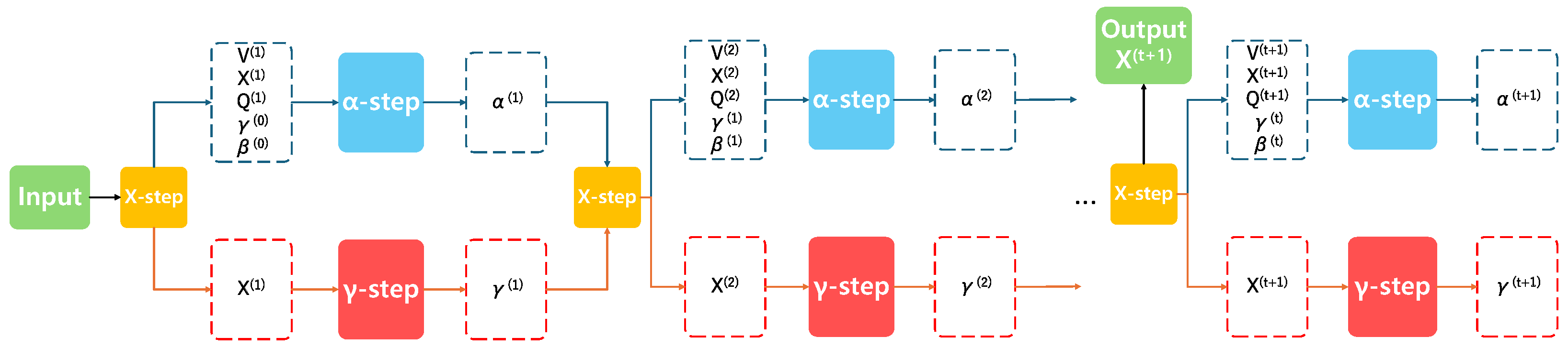
The iterative PC-2D-FIR-GEM solver naturally admits a stage-wise realization, and the overall architecture of PC-2D-FIR-GEM-Net is illustrated in Figure 2. By unfolding the iterative optimization procedure into a finite number of stages, we construct a model-driven deep unfolding network, termed PC-2D-FIR-GEM-Net. Specifically, each iteration of the analytical solver is mapped to one stage of the network. Let the state variables at the t-th stage be denoted as

$${\mathcal{S}}^{\left(t\right)}=\left\{{\mathbf{X}}^{\left(t\right)},{\mathit{\alpha }}^{\left(t\right)},{\gamma }^{\left(t\right)}\right\},$$

(36)

where ${\mathbf{X}}^{\left(t\right)}$ is the reconstructed image, ${\mathit{\alpha }}^{\left(t\right)}$ denotes the hyperparameter field, and ${\gamma }^{\left(t\right)}$ is the noise precision. Each stage includes steps for updating key parameters. Accordingly, the stage-wise mapping can be written as

$${\mathcal{S}}^{(t+1)}={\mathcal{F}}^{\left(t\right)}\left({\mathcal{S}}^{\left(t\right)};{\mathsf{\Theta }}^{\left(t\right)}\right),$$

(37)

where ${\mathcal{F}}^{\left(t\right)}(·)$ denotes the transformation of the t-th stage and ${\mathsf{\Theta }}^{\left(t\right)}$ denotes the trainable parameter set associated with that stage. In the proposed implementation, ${\mathsf{\Theta }}^{\left(t\right)}$ mainly includes the convolutional neural network kernels ${\mathbf{K}}^{\left(t\right)}$ used for generating the coupled precision field ${\mathit{\beta }}^{\left(t\right)}$, the Lipschitz constant $L_X^{\left(t\right)}$ and damping factor ${\lambda }^{\left(t\right)}$ in the $\mathbf{X}$-step, the learnable step size $r^{\left(t\right)}$ employed in the gradient-descent $\mathit{\alpha }$-step, and the auxiliary scaling coefficients within the softplus reparameterization. By optimizing all of these parameters in an end-to-end manner, the unfolded network is capable of dynamically adjusting both the update magnitudes and the structural prior strength according to the data distribution, thereby achieving high-quality imaging within very few stages.

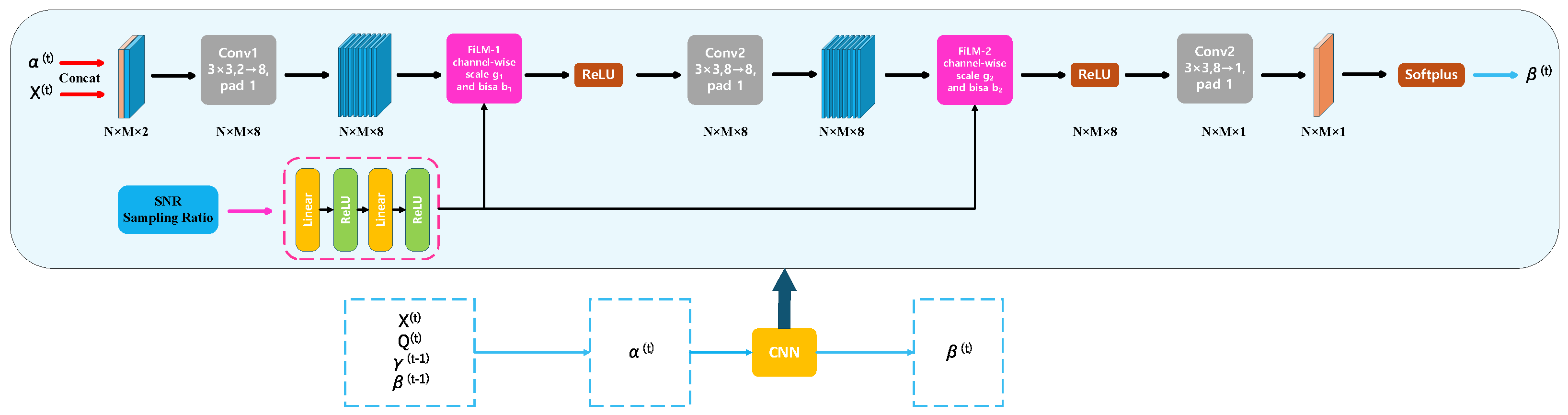
As described in (11), the coupled precision is constructed using a predefined neighborhood rule in the analytical model. Although effective, such a fixed formulation lacks the flexibility to capture complex spatial structures. To address this limitation, we introduce a learnable parameterization of the coupled prior by a CNN-based coupled-precision module. The CNN-based coupled-precision generation module is shown in Figure 3.

In the implementation, the CNN-based coupled-precision generator is a real-valued lightweight CNN. Although the ISAR image estimate $X^{\left(t\right)}$ is complex-valued in the inverse-free X-step, the CNN generator does not directly take the real and imaginary parts of $X^{\left(t\right)}$ as input; instead, the normalized power image $|X^{\left(t\right)}{|}^2$ is used as an amplitude-related structural feature. Specifically, the input tensor of the generator is defined as

$${\mathsf{\Xi }}^{\left(t\right)}=\mathrm{Concat}\left({\displaystyle \frac{{\alpha }^{\left(t\right)}}{\mathrm{mean}\left({\alpha }^{\left(t\right)}\right)+ϵ}},{\displaystyle \frac{|X^{\left(t\right)}{|}^2}{\mathrm{mean}\left(\right|X^{\left(t\right)}{|}^2)+ϵ}}\right)\in {\mathbb{R}}^{N\times M\times 2}.$$

(38)

Equation (11) gives the analytical pattern-coupled precision in the Bayesian model, whereas Equation (38) provides its learnable realization in the unfolded network. The CNN generator does not change the role of ${\beta }^{\left(t\right)}$ in the inverse-free X-step; it only replaces the fixed hand-crafted neighborhood rule with a data-adaptive precision parameterization. The coupled precision field is then obtained by

$${\beta }^{\left(t\right)}=\mathrm{Softplus}\left[G_{{\theta }_t}^{\mathrm{pre}}\left({\mathsf{\Xi }}^{\left(t\right)},{\mathbf{e}}_c\right)\right]+ϵ,$$

(39)

where $G_{{\theta }_t}^{\mathrm{pre}}(·)$ denotes the pre-Softplus CNN output and ${\mathbf{e}}_c$ is the embedding for the degradation condition. The condition embedding is generated from the sampling ratio and the estimated SNR by a two-layer fully connected encoder,

$${\mathbf{e}}_c=E_c\left({[{\rho }_s,{\displaystyle \frac{\widehat{\mathrm{SNR}}}{15}}]}^T\right),{\rho }_s=P/M,$$

(40)

where $E_c(·)$ has channel dimensions $2\to 16\to 16$. The detailed architecture of the CNN-based coupled-precision generator is summarized in

Table 1. Architecture of the CNN-based coupled-precision generator $G_{{\theta }_t}$.

Module	Input Size	Operation	Output Size	Activation
Input feature	$N\times M\times 2$	$\mathrm{Concat}({\overline{\alpha }}^{\left(t\right)},\overline{|X^{\left(t\right)}{|}^2})$	$N\times M\times 2$	–
Conv1	$N\times M\times 2$	$3\times 3$ Conv, 8 channels, padding 1	$N\times M\times 8$	–
FiLM-1	$N\times M\times 8,{\mathbf{e}}_c$	channel-wise scale and bias	$N\times M\times 8$	ReLU
Conv2	$N\times M\times 8$	$3\times 3$ Conv, 8 channels, padding 1	$N\times M\times 8$	–
FiLM-2	$N\times M\times 8,{\mathbf{e}}_c$	channel-wise scale and bias	$N\times M\times 8$	ReLU
Conv3	$N\times M\times 8$	$3\times 3$ Conv, 1 channel, padding 1	$N\times M\times 1$	Softplus

.

The two FiLM-type condition-modulation blocks are inserted after the first and second convolutional layers. For the l-th modulation block, the condition embedding ${\mathbf{e}}_c\in {\mathbb{R}}^{16}$ is linearly mapped to a channel-wise scale vector ${\mathbf{g}}_l\in {\mathbb{R}}^8$ and a bias vector ${\mathbf{b}}_l\in {\mathbb{R}}^8$. The modulated feature map is computed as

$${\mathbf{H}}_l^{\prime }={\mathbf{g}}_l\odot {\mathbf{H}}_l+{\mathbf{b}}_l,l=1,2,$$

(41)

where the scale and bias vectors are broadcast along the range and azimuth dimensions. The FiLM layers are initialized close to identity modulation, i.e., ${\mathbf{g}}_l\approx \mathbf{1}$ and ${\mathbf{b}}_l\approx \mathbf{0}$, so that the initial network remains close to the model-driven update.

The network uses $T=8$ unfolded stages. Unless otherwise specified, the parameters are not shared across stages. Each stage has its own CNN precision generator, FiLM modulation parameters, learned coupling kernel, damping factor, Lipschitz scaling coefficient, and $\alpha$-step size. This stage-specific design allows different stages to learn different update strengths and structural prior patterns during progressive reconstruction.

3.3. Training Strategy

The proposed PC-2D-FIR-GEM-Net is trained in an end-to-end manner using automatic differentiation. As described in Section 3.2, each unfolded stage maps the current state variables $\{X^{\left(t\right)},{\alpha }^{\left(t\right)},{\gamma }^{\left(t\right)}\}$ to the next stage through the differentiable PC-2D-FIR-GEM update. The trainable parameters include the CNN kernels used for coupled-precision generation, the Lipschitz-related parameter $L_X^{\left(t\right)}$, the damping factor ${\lambda }^{\left(t\right)}$, the $\alpha$-step size $r^{\left(t\right)}$, and the condition-modulation parameters. These parameters are jointly optimized through the computational graph of the unfolded network.

It should be noted that no manually implemented BP algorithm is required in practice. Although the model-driven update contains several interpretable modules, including the inverse-free X-step, the surrogate variance construction, the gradient-based $\alpha$-step, the closed-form $\gamma$-step, and the CNN-based coupled-precision generator, all of these operations are differentiable and can be handled by the automatic differentiation engine of the deep learning framework. Complex-valued variables are represented by their real and imaginary channels during implementation, while real-valued operations such as Softplus reparameterization, CNN convolution, FiLM-type condition modulation, and element-wise Bayesian updates are directly differentiable.

Let $\widehat{X}=X^{\left(T\right)}$ denote the final output of the unfolded network and $X_{\mathrm{ref}}$ the full-aperture supervisory reference image. The training objective consists of four components, namely, the complex-domain reconstruction loss, the magnitude-domain reconstruction loss, the stage-wise supervision loss, and the data consistency loss:

$$\mathcal{L}={\omega }_1{\mathcal{L}}_c+{\omega }_2{\mathcal{L}}_m+{\omega }_3{\mathcal{L}}_s+{\omega }_4{\mathcal{L}}_{dc}.$$

(42)

Specifically,

$${\mathcal{L}}_c={\displaystyle \frac{\parallel \widehat{X}-X_{\mathrm{ref}}{\parallel }_F^2}{\parallel X_{\mathrm{ref}}{\parallel }_F^2}},$$

(43)

$${\mathcal{L}}_m={\displaystyle \frac{\parallel |\widehat{X}|-|X_{\mathrm{ref}}{|\parallel }_F^2}{\parallel |X_{\mathrm{ref}}{|\parallel }_F^2}},$$

(44)

$${\mathcal{L}}_s={\displaystyle \frac{1}{T}}{\displaystyle \sum _{t=1}^T}{\displaystyle \frac{\parallel |X^{\left(t\right)}|-|X_{\mathrm{ref}}{|\parallel }_F^2}{\parallel |X_{\mathrm{ref}}{|\parallel }_F^2}},$$

(45)

and

$${\mathcal{L}}_{dc}={\displaystyle \frac{\parallel Y-{\mathcal{A}}_{\mathsf{\Omega }}(\widehat{X}){\parallel }_F^2}{{\parallel Y\parallel }_F^2}},$$

(46)

where the loss weights have been set to $({\omega }_1,{\omega }_2,{\omega }_3,{\omega }_4)=(0.7,0.3,0.1,0.01)$. Specifically, ${\mathcal{L}}_c=\parallel \widehat{\mathbf{X}}-{\mathbf{X}}_{\mathrm{ref}}{\parallel }_F^2/(\parallel {\mathbf{X}}_{\mathrm{ref}}{\parallel }_F^2)$ denotes the normalized complex-domain reconstruction error between the final output and the supervisory reference image; ${\mathcal{L}}_m=\parallel |\widehat{\mathbf{X}}|-|{\mathbf{X}}_{\mathrm{ref}}{|\parallel }_F^2/(\parallel |{\mathbf{X}}_{\mathrm{ref}}{|\parallel }_F^2)$ measures the normalized magnitude-domain consistency error; ${\mathcal{L}}_s=(1/T){\sum }_{t=1}^T\parallel |{\mathbf{X}}^{\left(t\right)}|-|{\mathbf{X}}_{\mathrm{ref}}{|\parallel }_F^2/(\parallel |{\mathbf{X}}_{\mathrm{ref}}{|\parallel }_F^2)$ provides stage-wise supervision for the intermediate outputs of the unfolded network; and ${\mathcal{L}}_{dc}=\parallel \mathbf{Y}-{\mathcal{A}}_{\mathsf{\Omega }}(\widehat{\mathbf{X}}){\parallel }_F^2/({\parallel \mathbf{Y}\parallel }_F^2)$ enforces data consistency between the reconstructed image and the sparse-aperture measurements under the forward model. The data consistency term constrains the reconstructed image to match the sparse-aperture measurements under the forward model, while the supervised reconstruction terms guide the network toward the full-aperture reference image. This training strategy preserves the physical consistency of the unfolded Bayesian update while allowing the stage-wise parameters and CNN-based coupled precision field to be optimized from data.

4. Experiments

This section describes experiments comprehensively evaluating the proposed method. Experiments were conducted on both simulated and measured ISAR data; simulated data were mainly used to quantify robustness under controlled sparse-aperture and low-SNR conditions, while measured data were mainly used to verify practical focusing capability and structural fidelity in real scenarios. Experimental results demonstrate that the proposed PC-2D-FIR-GEM-Net achieves excellent imaging performance with high efficiency.

4.1. Experimental Setup

To evaluate the reconstruction performance of the proposed PC-2D-FIR-GEM-Net, experiments were conducted on both simulated and measured ISAR datasets under sparse-aperture and low-SNR conditions. The compared methods include the conventional range-Doppler (RD) imaging method, 2D-FIR [29], PC-2D-FIR-GEM, PCSBL-GAMP-Net [28], and the proposed PC-2D-FIR-GEM-Net. Among them, PCSBL-GAMP-Net is introduced as a representative GAMP-based Bayesian unfolding baseline, whereas the proposed method unfolds an inverse-free GEM solver with CNN-based coupled-precision generation.

For a fair comparison, all methods were evaluated using the same sparse-aperture observations, sampling masks, and noisy input data under each test condition. The sparse-aperture observation was generated according to the forward model in Section 2, where the binary mask was applied to simulate incomplete azimuth-aperture measurements. Complex Gaussian noise was added to the full-sampled HRRP observation matrix after pulse compression. The sampling ratio and estimated SNR were used as auxiliary condition information for the proposed PC-2D-FIR-GEM-Net.

The quantitative evaluation is conducted using the image entropy (ENT), normalized mean square error (NMSE), structural similarity index measure (SSIM), and computational time (CT). ENT measures the concentration of the reconstructed image intensity distribution. Since an excessively sparse reconstruction may also lead to a low entropy value, NMSE and SSIM are further reported to evaluate reference-based reconstruction accuracy and structural fidelity. CT denotes the average computational time required by each method to reconstruct one image under the same hardware environment. All experiments were conducted on a workstation equipped with one NVIDIA H100 PCIe GPU. The PyTorch implementation used a single CUDA device for training and inference. For reproducibility, the random seed was fixed to 2026 for Python 3.12.12, NumPy 2.4.6, and PyTorch 2.7.1 during dataset loading, sparse-mask/noise generation, model initialization, and training.

For simulated data, the full-aperture RD image is used as the reference. For measured data, the full-aperture clean reconstruction is used as the reference after coordinate normalization. It should be noted that the full-aperture RD reference used for the measured data is not an ideal physical ground truth of the target reflectivity; since it is obtained through conventional RD processing after motion compensation and preprocessing, it may still contain RD-related characteristics such as finite mainlobe width, residual sidelobes, amplitude distribution bias, and possible preprocessing residuals. A supervised network trained with this reference may partially inherit these RD-like characteristics. For this reason, the reference-based quantitative metrics on measured data should be interpreted as consistency with the full-aperture RD reference rather than absolute physical reconstruction accuracy. In contrast, the simulated data provide known scattering-center information and are used for more controlled quantitative evaluation, including point-wise scattering center analysis.

The parameters of the proposed method are as follows: the network was trained using the Adam optimizer with an initial learning rate of $1\times {10}^{-4}$, weight decay of $1\times {10}^{-6}$, and batch size of 4. A cosine-annealing learning rate scheduler was adopted with $T_{max}=100$ and a minimum learning rate of $1\times {10}^{-6}$. With $T=8$, hidden channel number 8, and condition embedding dimension 16, each CNN precision generator contains 1353 trainable parameters. Each unfolded stage contains 1416 trainable parameters when including the stage-wise scalar parameters, learned $3\times 3$ coupling kernel, and condition modulators for ${\lambda }^{\left(t\right)}$, ${\eta }^{\left(t\right)}$, and ${\rho }^{\left(t\right)}$. Since the stages do not share parameters, the eight-stage network contains 11,684 trainable parameters in total, including the global condition encoder and the global initialization modulators. The stage-wise damping factor, Lipschitz constant, and $\mathit{\alpha }$-step size were initialized as ${\lambda }^{\left(0\right)}=0.90$, $L_X^{\left(0\right)}=1.0$, and $r^{\left(0\right)}=0.05$, respectively. The Gamma hyperparameters were fixed as $a_{\alpha }=1.1$, $b_{\alpha }={10}^{-6}$, $c_{\gamma }=1.0$, and $d_{\gamma }={10}^{-6}$.

In all experiments, the number of unfolding stages was fixed at $T=8$. This setting was selected based on an ablation study on the number of stages which tested the cases $T=4,6,8,10$, and 12. As T increased from 4 to 8, the image entropy decreased from 5.1436 to 5.0731, indicating improved focusing and background suppression; when T was further increased to 10 and 12, computation time continued to rise with increasing T, while image entropy increased to 5.1266 and 5.1468, respectively. This indicates that from an entropy perspective, deeper expansion stages do not further improve focusing quality but instead introduce additional computational overhead. Therefore, $T=8$ was selected as the setting that balances image focusing quality and inference efficiency.

4.2. SNR Estimation and Robustness to SNR-Condition Errors

In practical inference, the SNR input is not assumed to be an exact oracle value, instead being estimated from the observed data using a sparse-RD background median estimator. Let $X_0$ denote the initial sparse-RD image obtained from the observed sparse-aperture echo. The normalized magnitude image is first computed as

$$D(n,m)=20{log}_{10}\left({\displaystyle \frac{|X_0(n,m)|}{{max}_{n,m}\left|X_0(n,m)\right|+ϵ}}+ϵ\right).$$

(47)

The background-dominated set is selected as

$$\mathcal{B}=\{(n,m)\mid D(n,m)<T_{\mathrm{bg}}\},$$

(48)

where $T_{\mathrm{bg}}=-25$ dB in our implementation. The noise power is estimated by the median background power,

$${\widehat{P}}_n={median}_{(n,m)\in \mathcal{B}}{\left|X_0(n,m)\right|}^2,$$

(49)

and the signal power is estimated as

$${\widehat{P}}_s=max\left({\mathrm{mean}}_{n,m}{\left|X_0(n,m)\right|}^2-{\widehat{P}}_n,ϵ\right).$$

(50)

The estimated SNR is then given by

$${\widehat{\mathrm{SNR}}}_{\mathrm{dB}}=10{log}_{10}\left({\displaystyle \frac{{\widehat{P}}_s}{{\widehat{P}}_n+ϵ}}\right).$$

(51)

For the six representative measured samples, the adopted estimator achieves a mean absolute error (MAE) of 1.143 dB and a root mean square error (RMSE) of 1.394 dB, and all samples fall within $\pm 3$ dB of the nominal SNR labels. To further evaluate the influence of SNR-condition errors, we keep the trained checkpoint, input echo, sparse-aperture mask, and sampling ratio unchanged, only perturbing the SNR condition input by $\pm 3$ dB and $\pm 5$ dB. The metric differences are computed relative to the nominal-SNR case. Under $\pm 3$ dB perturbations, the maximum changes in normalized mean square error (NMSE), structural similarity index measure (SSIM), image entropy (ENT), and target-to-background ratio (TBR) are 0.003448, 0.001775, 0.016505, and 0.025675 dB, respectively. Even under $\pm 5$ dB perturbations, the corresponding maximum changes remain 0.006618, 0.003631, 0.029313, and 0.067999 dB. These results indicate that the SNR input is used as a coarse degradation condition variable rather than an exact oracle parameter.

4.3. Results on Simulated Data

The simulated ISAR dataset was first used to evaluate the proposed method under controlled sparse-aperture and low-SNR conditions. The carrier frequency was set to 10 GHz, the bandwidth was 600 MHz, and the pulse repetition frequency was 100 Hz. The simulation data were divided into a training set, validation set, and test set containing 800, 100, and 100 samples, respectively. There was no overlap between the three datasets, and each consisted of randomly generated scattered points. The imaging scene was discretized into a $256\times 256$ grid. The simulated target consisted of multiple clustered scattering blocks, which were used to verify whether the algorithms could preserve the structured scattering distribution under degraded observations.

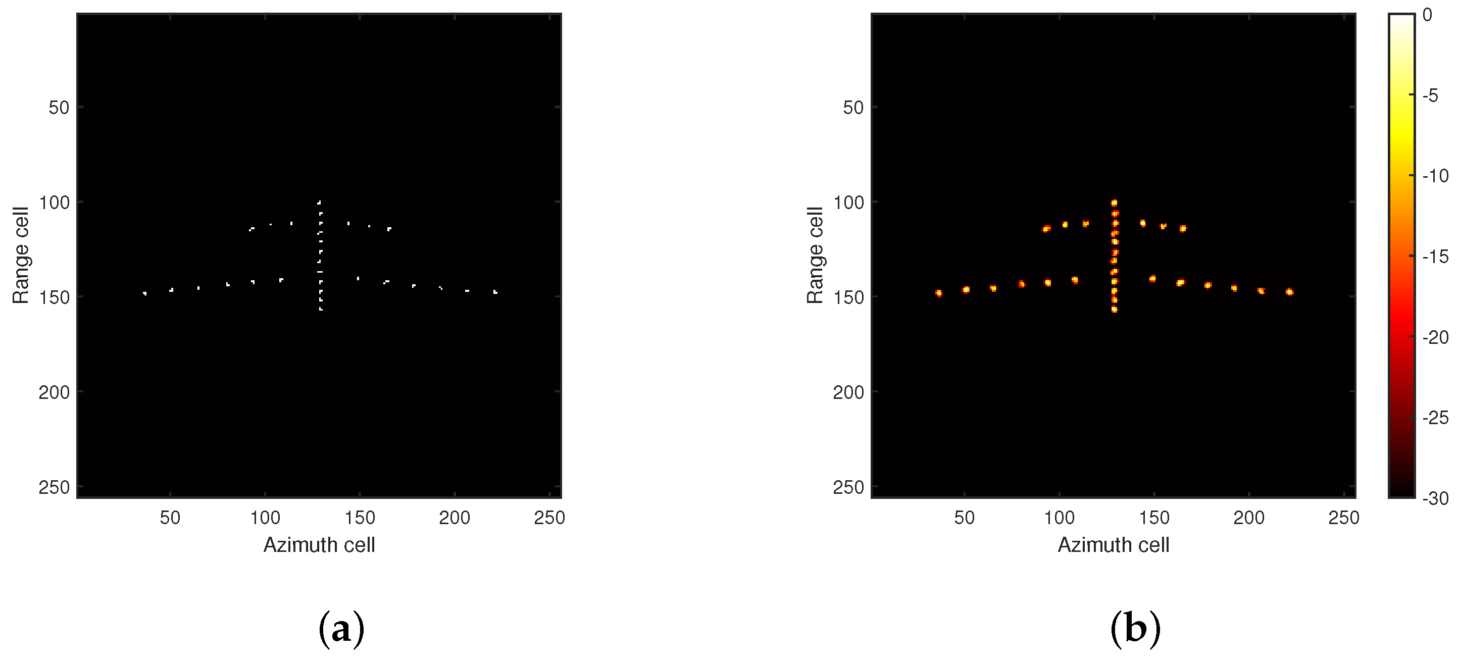
Figure 4 shows an example of the simulated dataset, including the ideal scatterer map and the corresponding full-aperture RD image. The ideal scatterer map provides the target scattering structure, while the full-aperture RD image serves as the supervisory reference image for visual comparison and supervised training. Compared with isolated scatterers, the clustered scattering structure is more suitable for evaluating the effectiveness of the pattern-coupled prior, since neighboring scatterers are statistically correlated in the image domain.

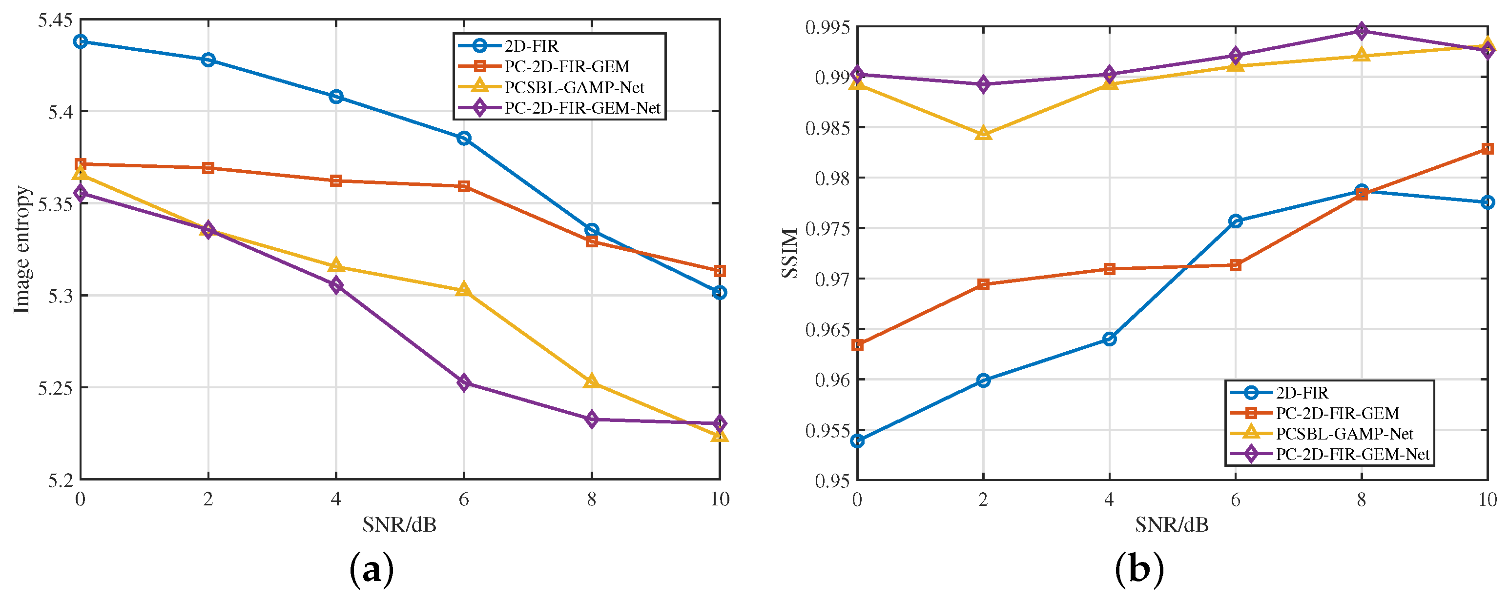
To verify the generalization capability of the proposed method, additional experiments were conducted on the simulated test data under different sparse sampling conditions. Specifically, for each input SNR and each sparse sampling ratio, 100 independent samples were used for evaluation, and the corresponding quantitative metrics were averaged. Figure 5 shows the image entropy and SSIM results under input SNRs from 0 dB to 10 dB. Lower image entropy indicates a more compact reconstructed image, while higher SSIM indicates better structural similarity with the reference image.

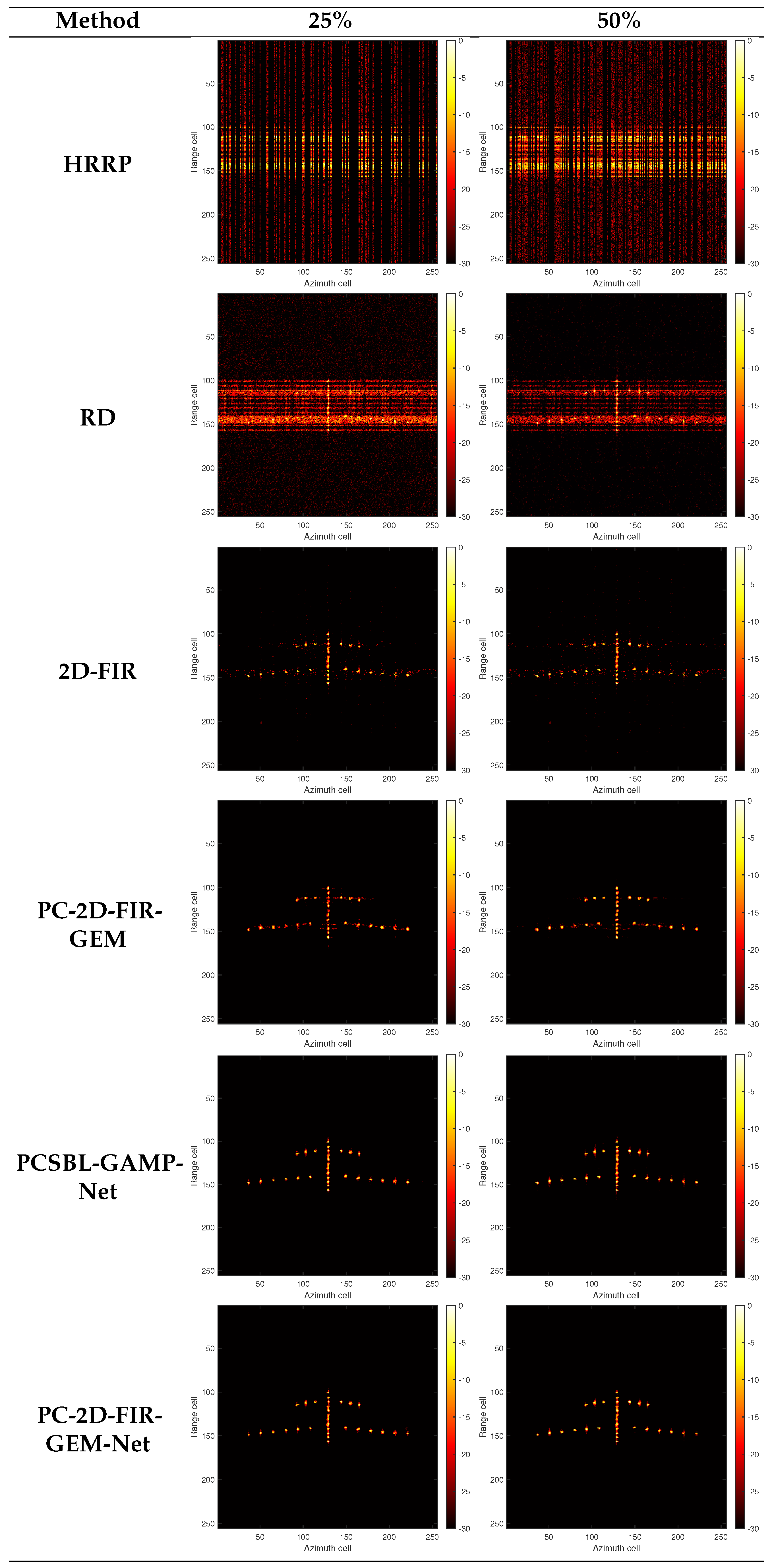
To evaluate the robustness to sparse-aperture sampling, the input SNR was fixed at 5 dB and two sampling ratios were tested, $25\%$ and $50\%$. The reconstructed images are shown in Figure 6, and the corresponding ENT, NMSE, SSIM, and CT values are reported in

Table 2. Numerical performance of different algorithms on simulated airplane data at 5 dB with different sampling ratios.

Sampling Ratio	Algorithm	ENT	NMSE	SSIM	CT (s)
25%	RD	10.7022	2.8943	0.3105	0.0012
	2D-FIR	5.2837	0.2063	0.9103	0.9402
	PC-2D-FIR-GEM	5.2543	0.1816	0.9530	0.4083
	PCSBL-GAMP-Net	5.2160	0.0627	0.9903	0.1631
	PC-2D-FIR-GEM-Net	5.2128	0.0584	0.9909	0.0759
50%	RD	10.7139	2.7280	0.1159	0.0009
	2D-FIR	5.3537	0.0887	0.9575	0.9635
	PC-2D-FIR-GEM	5.3064	0.0589	0.9716	0.4114
	PCSBL-GAMP-Net	5.2649	0.0302	0.9932	0.1589
	PC-2D-FIR-GEM-Net	5.2476	0.0327	0.9889	0.0802

. The CT was calculated under each testing condition by 50 Monte Carlo trials; the standard deviations of 2D-FIR, PC-2D-FIR-GEM, PCSBL-GAMP-Net, and the proposed PC-2D-FIR-GEM-Net were 0.0142 s, 0.0069 s, 0.0034 s, and 0.0039 s, respectively. As shown in Figure 6, the RD result suffers from severe defocusing and sidelobe artifacts when only sparse-aperture measurements are available. This degradation becomes more obvious under the $25\%$ sampling ratio, where the available azimuth information is highly incomplete.

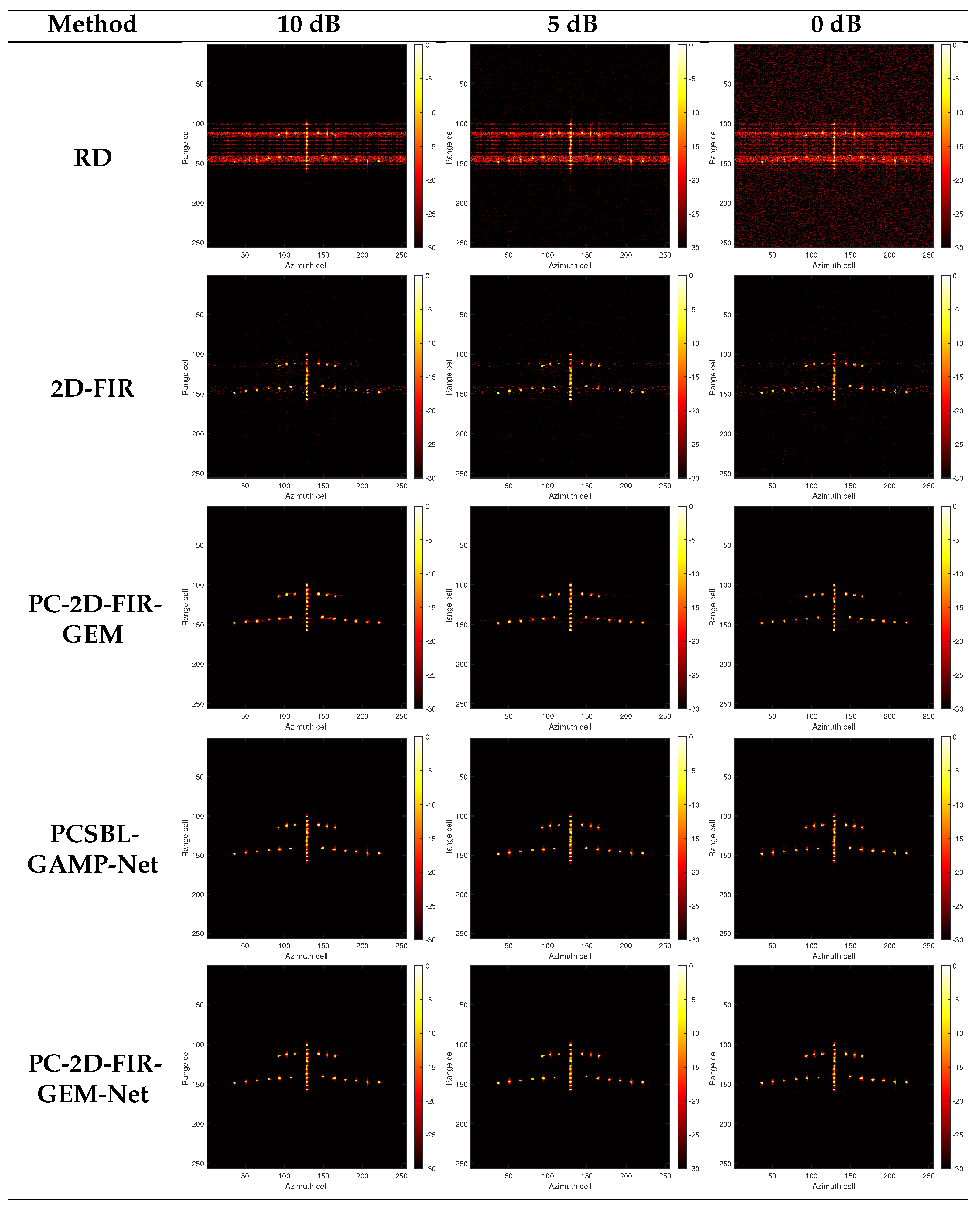
To further evaluate robustness to noise, the sampling ratio was fixed at $50\%$ and the input SNR was set to 10, 5, and 0 dB, respectively. The visual results are shown in Figure 7 and the numerical results are listed in

Table 3. Numerical performance of different algorithms on simulated airplane data at 50% sampling ratio with different SNRs.

SNR	Algorithm	ENT	NMSE	SSIM	CT (s)
$10\mathrm{dB}$	RD	10.4957	1.0110	0.4794	0.0010
	2D-FIR	5.3048	0.0944	0.9805	0.9683
	PC-2D-FIR-GEM	5.2688	0.0570	0.9825	0.4075
	PCSBL-GAMP-Net	5.2444	0.0354	0.9946	0.2120
	PC-2D-FIR-GEM-Net	5.2405	0.0154	0.9946	0.0900
$5\mathrm{dB}$	RD	10.7139	2.7280	0.1159	0.0009
	2D-FIR	5.3537	0.0887	0.9575	0.9635
	PC-2D-FIR-GEM	5.3064	0.0589	0.9716	0.4114
	PCSBL-GAMP-Net	5.2649	0.0302	0.9932	0.1589
	PC-2D-FIR-GEM-Net	5.2476	0.0327	0.9889	0.0802
$0\mathrm{dB}$	RD	10.8536	3.9442	0.1353	0.0011
	2D-FIR	5.4153	0.1243	0.9644	0.9569
	PC-2D-FIR-GEM	5.3691	0.1131	0.9658	0.4245
	PCSBL-GAMP-Net	5.3601	0.1027	0.9889	0.1700
	PC-2D-FIR-GEM-Net	5.3483	0.0727	0.9903	0.0769

. When the SNR decreases, the RD image becomes increasingly contaminated by noise-like artifacts, making it easy for weak scattering structures to become obscured. Although 2D-FIR and PC-2D-FIR-GEM improve image focusing compared with RD, residual false scatterers and background fluctuations still remain under low-SNR conditions. PCSBL-GAMP-Net provides strong structural reconstruction owing to its Bayesian unfolding mechanism. The proposed PC-2D-FIR-GEM-Net further maintains a compact target structure and clean background while requiring less computational time. When considering ENT, NMSE, SSIM, and CT jointly, the proposed method shows stable reconstruction capability across different SNR levels and is suitable for fast ISAR imaging under sparse and noisy observations.

The single-scatterer PSLR and ISLR results in

Table 4. Evaluation of peak sidelobe ratio and integrated sidelobe ratio for a single scatterer.

SNR	Sampling Ratio	Algorithm	PSLR (dB)	ISLR (dB)
$10\mathrm{dB}$	25%	2D-FIR	−8.1101	−0.6787
		PC-2D-FIR-GEM	−8.6254	−2.5662
		PCSBL-GAMP-Net	−9.2502	−4.2218
		PC-2D-FIR-GEM-Net	−9.1609	−7.5321
	50%	2D-FIR	−8.1851	−4.4057
		PC-2D-FIR-GEM	−9.5839	−6.1442
		PCSBL-GAMP-Net	−10.2917	−6.9595
		PC-2D-FIR-GEM-Net	−11.1621	−8.5843
$5\mathrm{dB}$	25%	2D-FIR	−8.6582	−2.4888
		PC-2D-FIR-GEM	−8.3288	−5.5370
		PCSBL-GAMP-Net	−11.0249	−7.1631
		PC-2D-FIR-GEM-Net	−11.8921	−8.3910
	50%	2D-FIR	−9.3055	−3.8965
		PC-2D-FIR-GEM	−9.3341	−3.0274
		PCSBL-GAMP-Net	−11.4337	−6.4957
		PC-2D-FIR-GEM-Net	−11.1353	−8.0526
$0\mathrm{dB}$	25%	2D-FIR	−7.9989	−1.9387
		PC-2D-FIR-GEM	−9.4237	−3.3335
		PCSBL-GAMP-Net	−10.5010	−5.1830
		PC-2D-FIR-GEM-Net	−11.5828	−6.5089
	50%	2D-FIR	−8.5764	−1.8705
		PC-2D-FIR-GEM	−9.5403	−5.3407
		PCSBL-GAMP-Net	−10.3374	−5.0630
		PC-2D-FIR-GEM-Net	−10.6660	−5.8201

further evaluate the local sidelobe suppression capability of different methods. The 2D-FIR method improves image sparsity to some extent, but its fixed reconstruction model has limited ability to suppress sparse aperture-induced sidelobes, grating lobes, and local residual artifacts around individual scattering centers. Although PC-2D-FIR-GEM introduces a pattern-coupled prior to exploit neighborhood dependencies, it is still based on conventional iterative optimization with limited data adaptation capability; as a result, residual weak peaks and background fluctuations may still accumulate in the sidelobe region, leading to unsatisfactory PSLR and ISLR values. In contrast, PCSBL-GAMP-Net achieves favorable PSLR and ISLR performance due to its unfolded block-sparse Bayesian structure. Because PC-2D-FIR-GEM-Net unfolds the iterative reconstruction process into a trainable network and learns the local coupling precision and stage-wise parameters from data, it can more effectively suppress local pseudo-peaks, interference from neighboring scatterers, and sparse-aperture sidelobe residuals.

4.4. Results on Measured Data

The results on measured data further verify the practical applicability of the proposed method. Compared with the results for simulated data, the measured ISAR echoes contain more complicated scattering fluctuations, residual phase errors, and background interference. Under such conditions, RD and 2D-FIR are more likely to produce blurred structures and false scatterers. PC-2D-FIR-GEM improves the reconstruction by introducing pattern-coupled Bayesian modeling, while PCSBL-GAMP-Net benefits from model-driven unfolding and provides better structural preservation than purely iterative sparse reconstruction methods. The proposed PC-2D-FIR-GEM-Net achieves clear target reconstruction under both low-SNR and sparse-aperture conditions. By jointly considering ENT, NMSE, SSIM, and CT, the proposed method provides a favorable balance between imaging quality and reconstruction speed.

The experimental data were collected during two Yak-42 flight missions. To prevent data leakage, the training, validation, and test sets were separated at the source-echo level prior to generating sparse apertures and noisy observations. Specifically, the continuous echoes from the two flight missions were first divided into full-aperture base echo windows based on slow time series, ensuring that adjacent windows did not contain continuous pulse sequences. Each base echo window was assigned to only one of the training, validation, or test sets. After completing this source-level partitioning, sparse aperture masks and noise perturbations were generated independently for each subset. Consequently, different degraded versions generated from the same original full-aperture echo did not appear in different subsets. The final real-world data partition consisted of 1914 training samples, 264 validation samples, and 264 test samples. The validation set was used solely for model selection and early stopping mechanisms, while the test set was used exclusively for final evaluation. No test samples were used during training, validation, hyperparameter selection, or calibration of the signal-to-noise ratio (SNR) estimator. This partitioning strategy ensures that the reported performance evaluation results are based on the ability to reconstruct unseen echo bands rather than on different degraded versions of the same original echo. After standard preprocessing, the full-aperture echoes were used to generate supervisory reference images, while degraded inputs were produced by applying sparse-aperture masks and adding complex Gaussian noise. The full-aperture image was used as the reference image for supervised training and visual comparison. Therefore, the measured data experiment mainly focuses on structural preservation, background suppression, and computational efficiency rather than absolute pixel-wise recovery accuracy.

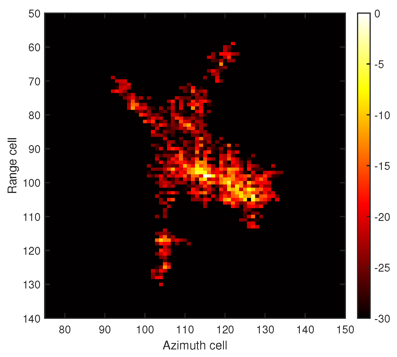
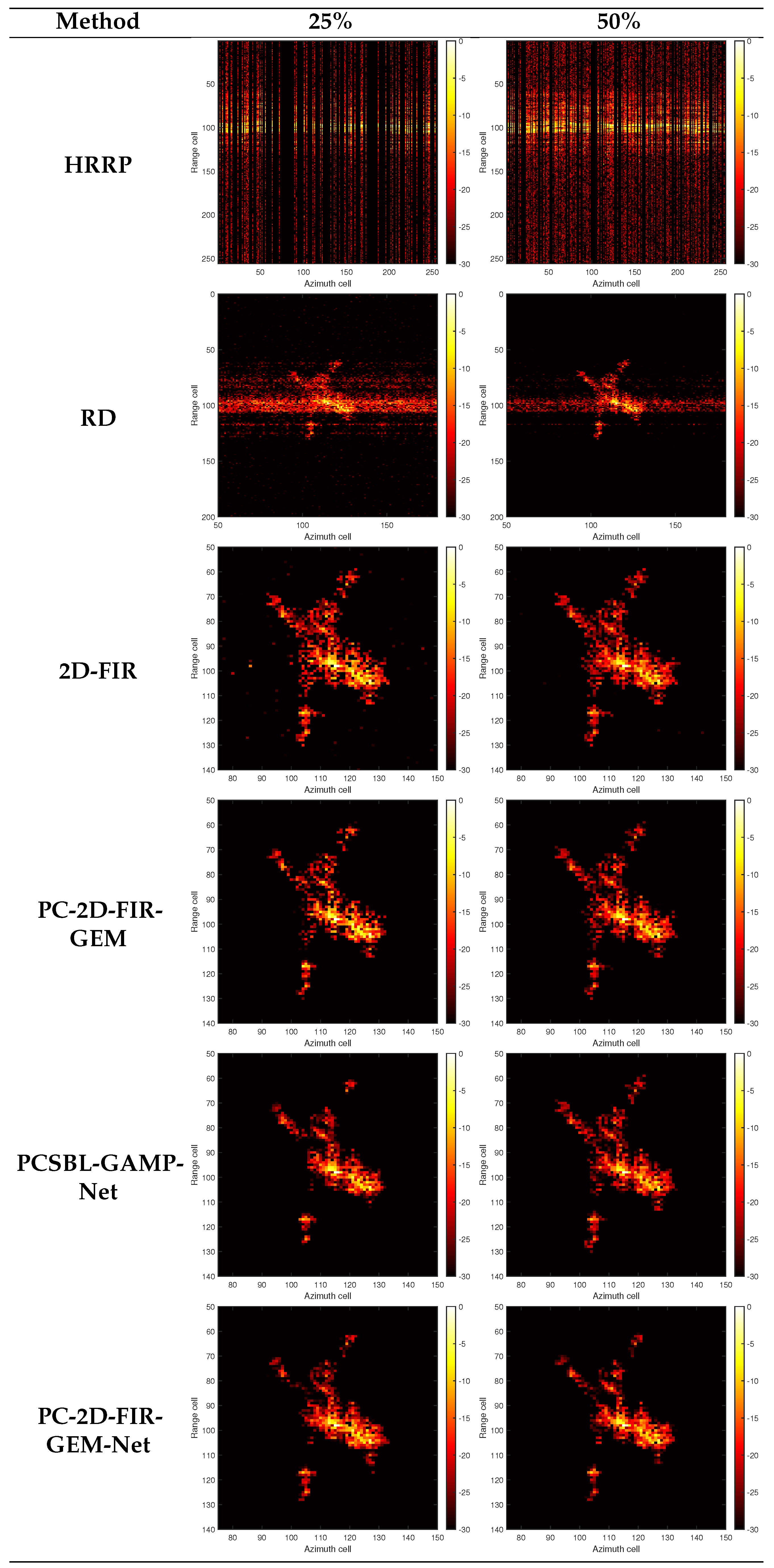
Figure 8 shows the full-aperture RD imaging result, which is used as the reference for visual comparison. Figure 9 presents the reconstructed images of different methods under sparse-aperture measured data conditions. The input SNR was fixed at 5 dB, and two sampling ratios of $25\%$ and $50\%$ were considered. The corresponding quantitative results are reported in

Table 5. Numerical performance of different algorithms on measured airplane data at 5 dB with different sampling ratios.

Sampling Ratio	Algorithm	ENT	NMSE	SSIM	CT (s)
25%	RD	10.7095	2.7873	0.0890	0.0011
	2D-FIR	5.8183	0.1450	0.6060	0.8617
	PC-2D-FIR-GEM	5.2621	0.1148	0.6400	0.3973
	PCSBL-GAMP-Net	5.2431	0.1136	0.8708	0.0872
	PC-2D-FIR-GEM-Net	5.2427	0.0957	0.9370	0.0795
50%	RD	10.7123	2.2484	0.1820	0.0011
	2D-FIR	6.3027	0.2025	0.5660	0.8942
	PC-2D-FIR-GEM	5.3885	0.0962	0.6370	0.3853
	PCSBL-GAMP-Net	5.2897	0.1277	0.8946	0.1090
	PC-2D-FIR-GEM-Net	5.1807	0.0820	0.9320	0.0790

, including ENT, NMSE, SSIM, and CT. Under the $25\%$ sampling ratio, the results for conventional RD suffer from severe background artifacts and discontinuous target structures because of the significant loss of azimuth-aperture information. The methods based on sparse reconstruction improve the focusing quality to different degrees. Specifically, 2D-FIR enhances image sparsity, PC-2D-FIR-GEM further exploits the pattern-coupled prior to improve structural compactness, and PCSBL-GAMP-Net provides a model-driven unfolding baseline with improved structural reconstruction. In comparison, the proposed PC-2D-FIR-GEM-Net preserves the main target scattering structure more stably while suppressing background artifacts and maintaining a low computational cost. These results indicate that the proposed method can effectively reconstruct measured ISAR target structures under low-SNR and sparse-aperture conditions.

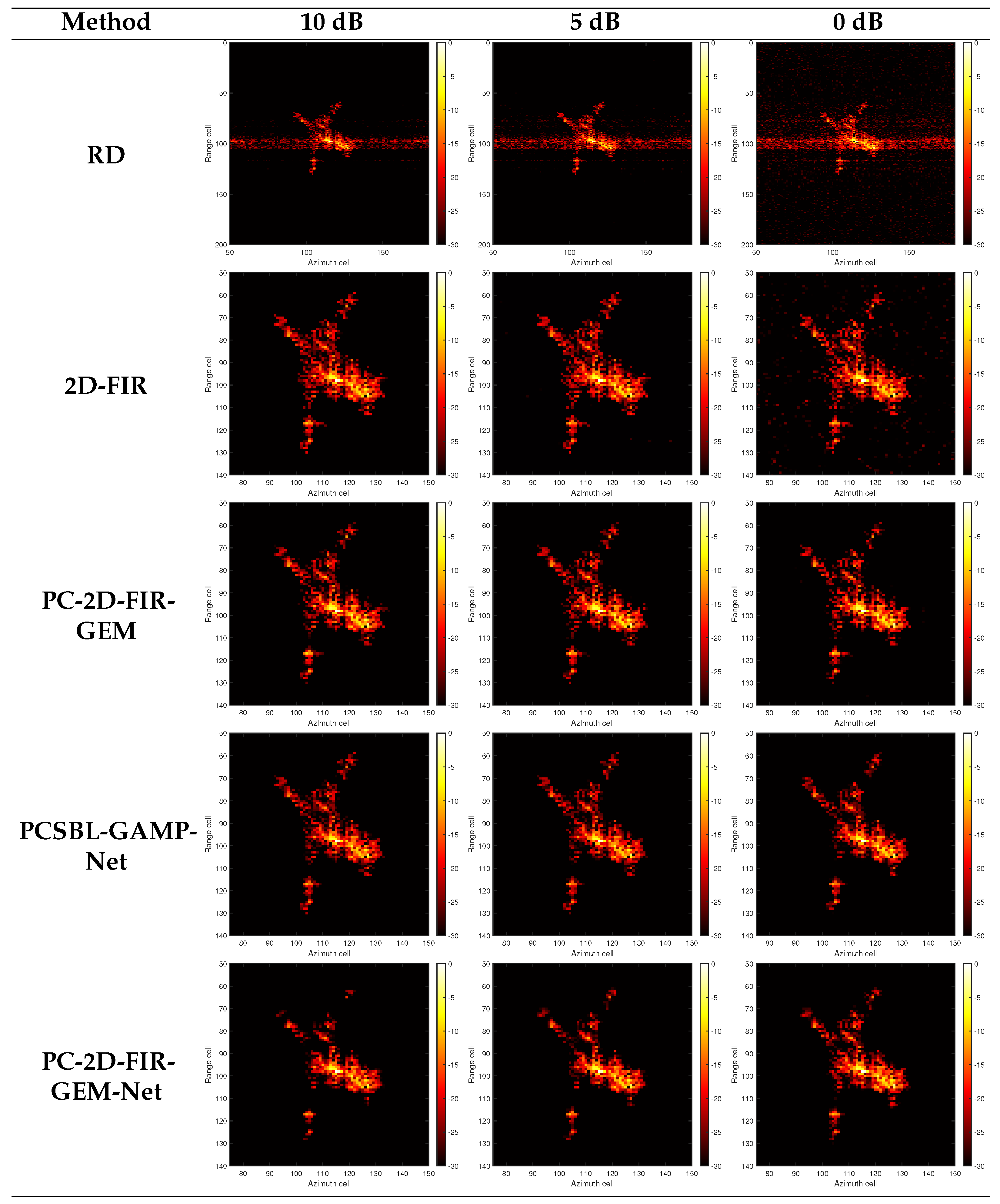
Figure 10 presents the imaging results for measured data under different SNR levels, where the sampling ratio was fixed at $50\%$. As the SNR decreases from 10 dB to 0 dB, the imaging difficulty increases because the sparse-aperture observations are further contaminated by noise. The RD and 2D-FIR results exhibit more visible background interference and false scatterers under low-SNR conditions. PC-2D-FIR-GEM and PCSBL-GAMP-Net improve the reconstruction quality by introducing Bayesian structural modeling and model-driven unfolding, respectively. The proposed PC-2D-FIR-GEM-Net further maintains clear target scattering structures across different SNR levels and effectively suppresses background artifacts. The visual results demonstrate that the proposed method has stable reconstruction capability for measured ISAR data under both sparse sampling and low-SNR degradation.

The quantitative results in Table 5 and

Table 6. Numerical performance of different algorithms on measured airplane data at 50% sampling ratio with different SNRs.

SNR	Algorithm	ENT	NMSE	SSIM	CT (s)
$10\mathrm{dB}$	RD	10.4934	0.9929	0.2550	0.0011
	2D-FIR	5.9230	0.1387	0.6140	0.8877
	PC-2D-FIR-GEM	5.3236	0.0495	0.6340	0.3828
	PCSBL-GAMP-Net	5.3426	0.0823	0.8980	0.1299
	PC-2D-FIR-GEM-Net	5.0735	0.1077	0.8890	0.0736
$5\mathrm{dB}$	RD	10.7123	2.2484	0.1820	0.0011
	2D-FIR	6.3027	0.2025	0.5660	0.8942
	PC-2D-FIR-GEM	5.3885	0.0962	0.6370	0.3853
	PCSBL-GAMP-Net	5.2897	0.1277	0.8946	0.1090
	PC-2D-FIR-GEM-Net	5.1807	0.0820	0.9320	0.0790
$0\mathrm{dB}$	RD	10.8491	2.4504	0.1270	0.0012
	2D-FIR	7.5430	0.2542	0.4390	0.8347
	PC-2D-FIR-GEM	5.4196	0.0916	0.6330	0.3800
	PCSBL-GAMP-Net	5.3418	0.0937	0.9006	0.1362
	PC-2D-FIR-GEM-Net	5.3180	0.0758	0.9630	0.0655

further support the visual comparison. Since a single metric cannot fully characterize the imaging quality, the evaluation jointly considers ENT, NMSE, SSIM, and CT. To further assess the statistical stability of the computational efficiency, the runtime of each method was repeatedly measured over 50 independent runs under the same hardware and software configuration. The CT standard deviations of 2D-FIR, PC-2D-FIR-GEM, PCSBL-GAMP-Net, and the proposed PC-2D-FIR-GEM-Net were 0.0127 s, 0.0077 s, 0.0061 s, and 0.0052 s, respectively. The small standard deviations indicate that the runtime measurements are stable across repeated trials. Compared with conventional iterative methods, the methods based on unfolded networks not only reduce the average computational time but also exhibit stable runtime fluctuations, further confirming their practical computational efficiency. Although RD has the lowest computational cost owing to its FFT-based implementation, its image quality degrades significantly under sparse and noisy observations. Compared with iterative Bayesian reconstruction methods and the GAMP-based unfolding baseline, PC-2D-FIR-GEM-Net achieves a favorable overall balance among image focusing quality, target structural fidelity, background suppression, and computational efficiency. These results confirm that the proposed method is suitable for fast and reliable high-resolution ISAR imaging under practical low-SNR and sparse-aperture conditions.

4.5. Computational Complexity

Let $D=NM$ denote the number of image pixels, where N and M are the range and azimuth dimensions, respectively. The proposed PC-2D-FIR-GEM-Net has a fixed-stage inference structure with T unfolded stages. In each stage, the dominant computation comes from the forward and adjoint imaging operations in the inverse-free X-step. When the range and azimuth imaging operators are implemented by FFT/IFFT-type operations, this part has complexity $\mathcal{O}(DlogD)$. The subsequent X-update, $\alpha$-update, $\gamma$-update, damping operation, and surrogate variance construction are all element-wise operations with complexity $\mathcal{O}\left(D\right)$. The CNN-based coupled-precision generator is lightweight; for a convolution kernel of size $k\times k$ and hidden channel number C, the three convolutional layers introduce approximately $\mathcal{O}\left(k^2(C^2+3C)D\right)$ operations, while the FiLM-type condition modulation and fully connected condition encoder only introduce minor additional overhead. Therefore, the total inference complexity of the proposed network can be written as $\mathcal{O}\left(TDlogD+T{k}^2(C^2+3C)D\right)$.

In our implementation, $T=8$, $k=3$, and $C=8$, so the CNN-related cost remains small and the overall complexity is dominated by a fixed number of forward and adjoint imaging operations. More importantly, the proposed inference procedure does not require large-scale matrix inversion or convergence-dependent iterative optimization. Once the network is trained, the number of computational stages is fixed; all major operations, including FFT-type transforms, element-wise Bayesian updates, and convolutional precision generation, can be efficiently parallelized on modern hardware. This fixed-stage, inverse-free, and parallelizable structure explains the fast imaging time achieved by the proposed method in our experiments.

5. Conclusions

This article proposes PC-2D-FIR-GEM-Net, a method for high-resolution ISAR imaging under low-SNR and sparse-aperture conditions. A pattern-coupled hierarchical Bayesian model is first established to exploit the spatial clustering characteristics of ISAR scatterers. Then, an inverse-free GEM inference scheme is developed to avoid large-scale matrix inversion and improve computational efficiency. By unfolding the iterative PC-2D-FIR-GEM solver into a staged network, the proposed method combines the physical interpretability of Bayesian inference with the adaptive representation capability of CNN-based coupled-precision generation. Experimental results on both simulated and measured ISAR data demonstrate that the proposed method can effectively suppress noise and sparse-aperture artifacts, preserve target scattering structures, and achieve lower image entropy and shorter computational time than the compared methods. These results verify the effectiveness and efficiency of the proposed PC-2D-FIR-GEM-Net for robust ISAR imaging in challenging observation scenarios.