DPMSCH-Net: A Dual Prior-Guidance Multi-Scale SSM-CNN Hybrid Network with Manifold Constraints for Hyperspectral Image Classification Under Small-Sample Conditions

Highlights

What are the main findings?

• DPMSCH-Net with prior-guided DMB captures spatial–spectral information under data scarcity, and SupCon regularizationmitigates feature collapse through manifold constraints.
• It achieves state-of-the-art five-shot classification performance across HanChuan, HongHu, and XiongAn datasets.

What are the implications of the main finding?

• It offers a robust framework for real-world agricultural HSI monitoring with minimal annotation costs.
• It demonstrates the potential of injecting physical priors into sequence modeling for few-shot tasks.

Abstract

Hyperspectral images (HSIs) demonstrate significant potential in agricultural applications, but conventional classification methods face challenges in adequately extracting complex spatial–spectral features. While deep learning approaches provide powerful representational capabilities, standard homogeneous architectures often show limitations in effectively capturing multi-scale contexts. Additionally, extreme label scarcity increases the difficulty of identifying central targets and informative spectral bands, while the absence of explicit feature-space constraints may render models more susceptible to feature collapse and overfitting. To this end, we propose a multi-scale asymmetric architecture named the dual prior-guidance multi-scale SSM-CNN hybrid network (DPMSCH-Net) for hyperspectral image classification (HSIC) based on few-shot learning (FSL) under an extreme scenario of only five labeled samples per class. Specifically, to capture multi-scale contexts, DPMSCH-Net employs a dual Mamba block (DMB) and a hierarchical context module (HCM) in the first two high-resolution stages, and the CNN branch in the third lowest-resolution stage for enhancing spatial–spectral representation. Subsequently, to extract discriminative features from limited samples, DMB is guided by the Gaussian spatial prior, while the PCA-inspired spectral decay prior provides statistical guidance for learning discriminative spectral representations. Finally, to further optimize the feature-space structure, supervised contrastive (SupCon) regularization is introduced to impose strict manifold constraints via implicit hard sample mining. Extensive five-shot experiments on the HongHu, HanChuan, and XiongAn datasets demonstrate that DPMSCH-Net achieves an average Overall Accuracy (OA) of 88.25%, 82.90%, and 67.35%, outperforming SOTA methods by a significant margin.

1. Introduction

Hyperspectral images (HSIs) contain rich spectral–spatial features, giving them high value in agricultural application [1], environmental monitoring [2], and urban development [3]. However, application of HSI in agriculture is bottlenecked by the exorbitant cost of pixel-level annotations. Given the pronounced heterogeneity of field crops, their spectral signatures vary substantially across phenological stages and local microenvironments. As a result, reliable annotations rely on intensive, expert-dependent fieldwork, which essentially rules out large-scale labeling campaigns. To address this challenge, few-shot learning for hyperspectral image classification (FSL-HSIC) has emerged. This paradigm seeks to effectively extract discriminative spectral–spatial representations from an extremely limited number of labeled samples, thereby producing more reliable predicted classification maps.

Early traditional hyperspectral image classification (HSIC) methods such as support vector machines (SVMs) [4], k-nearest neighbor (KNN) [5], and random forests (RFs) [6] often struggle with the “curse of dimensionality” and inherent feature redundancy when applied to HSI. Although, these models offer high interpretability, these shallow models struggle to fully exploit the complex non-linear spatial–spectral relationships inherent in high-dimensional data, limiting their discriminative capability in complex scenes. Deep learning architectures perfectly compensate for this defect through their powerful non-linear modeling capabilities, yielding great success in capturing and extracting robust spatial–spectral characteristics from high-dimensional hyperspectral (HS) data [7]. Specifically, representative approaches—ranging from classic CNN frameworks such as SSRN [8] and DFFN [9] to emerging Transformer models like GSC-ViT [10] and SpectralFormer [11]—have achieved remarkable success in fully supervised HSIC. However, their data-driven nature makes them susceptible to severe overfitting when labeled samples are scarce, as their massive parameter spaces tend to memorize limited training instances rather than learning generalizable features. Due to the prohibitive cost of pixel-level annotation, FSL-HSIC has emerged as a critical research problem, where existing methods can be grouped into three main paradigms: meta-learning, metric learning, and data augmentation.

Meta-learning-based methods are trained on data-rich base classes to learn transferable representations and rapid adaptation capabilities, thereby enabling strong generalization on novel classes with limited samples. To model the inherent uncertainty in data-scarce scenarios, Zhang et al. [12] proposed a Bayesian meta-learning framework that infers task-specific parameters from probability distributions. Building upon optimization strategies, Li et al. [13] introduced a regularized fine-tuning mechanism into the meta-learning paradigm to effectively prevent overfitting during the rapid adaptation stage. More recently, to construct a more discriminative feature space, Wang et al. [14] designed ${\mathrm{I}}^2$MEP-Net to refine the spatial–spectral representations. While these methods establish robust frameworks, they often overlook the spectral–spatial domain shifts between base and novel classes. In applications, this discrepancy degrades the learned features and limits their actual generalization capability.

Metric learning approaches tackle the FSL challenge by mapping samples into a discriminative embedding space, where instances from the same class are clustered together and those from different classes are separated. For HSI classification, various spatial–spectral metric networks have been designed to capture data dependencies. Specifically, Gao et al. [15] introduced a deep relation network to automatically learn non-linear similarity representations between HS patches. This paradigm was further advanced by Zeng et al. [16], who proposed a multistage relation network with a dual-metric mechanism to capture more intricate spatial–spectral relations. Additionally, Deng et al. [17] utilized contrastive optimization strategies to explicitly enhance the discriminative power of the extracted features. However, significant spectral–spatial domain shifts in complex agricultural scenes often distort these static distance metrics, limiting their generalization capability.

Data augmentation strategies offer a direct solution to data scarcity by expanding the training set through sample synthesis, recombination, or transformation. In the HSI domain, generating realistic spatial–spectral features is critical. Specifically, generative adversarial networks (GANs) have been successfully employed by Zhu et al. [18] to synthesize high-fidelity HS patches and enrich data diversity. Alternatively, data recombination strategies, such as the deep pixel-pair method proposed by Li et al. [19], significantly expand the training volume by pairing limited available samples to construct a more robust feature space. Furthermore, to enhance model robustness against spatial variations, Nalepa et al. [20] systematically explored training- and test-time spatial–spectral transformations. Additionally, interpolation-based techniques like Mixup [21] have been widely adapted in HSI classification to create virtual samples and smooth decision boundaries. However, bounded by the distribution of limited base classes, these generated samples struggle with significant spectral–spatial domain shifts in agricultural scenes, often amplifying data biases and limiting generalization.

Although existing methods have laid a technical foundation for FSL-HSIC, they still face several challenges under extreme data scarcity. Homogeneous architectures typically employ uniform feature extraction mechanisms, lacking the ability to differentially model features at different resolutions, which limits the full exploitation of multi-scale spatial–spectral contextual information. Although prior information has been incorporated through attention mechanisms and feature re-weighting to enhance feature expressiveness, these priors are typically introduced through model-driven mechanisms, with relatively limited exploitation of the inherent spatial distribution and spectral statistical properties of HS data. Likewise, although contrastive and metric learning have been adopted to regularize the feature space, they often rely on complex sample relationship modeling or additional optimization strategies, making robust feature-space regularization under extremely few-shot conditions challenging and consequently limiting model generalization.

To address these limitations, we proposed a dual prior-guidance multi-scale SSM-CNN hybrid network (DPMSCH-Net) tailored for FSL-HSIC. Unlike traditional architectures, inspired by the success of hierarchical feature fusion in related spatial–spectral tasks [22], our model adopts a multi-scale asymmetric hierarchical design, integrating a hierarchical context module (HCM) for fine-grained spatial feature aggregation to effectively handle complex agricultural land covers. To better exploit the intrinsic physical characteristics of HS data, we design a dual Mamba block (DMB) guided by adaptive Gaussian spatial and PCA-inspired spectral decay priors. This enables the network to precisely focus on central targets while emphasizing informative spectral representations, thereby extracting highly discriminative spatial–spectral features. Furthermore, to further enhance feature-space discrimination under extremely limited supervision, we introduce a supervised contrastive (SupCon) regularization [23] mechanism. Through implicit hard sample mining, this regularizer effectively remodels the feature space without tedious pair construction, significantly enhancing intra-class compactness and inter-class dispersion.

The main contributions of this paper are summarized as follows:

(1)

We propose DPMSCH-Net, an asymmetric SSM–CNN hybrid backbone designed for few-shot learning for hyperspectral image classification. By progressively integrating dual Mamba blocks (DMBs), hierarchical context modules (HCMs), and CNNs across different decreasing resolutions, the network effectively captures local-to-global spatial–spectral contexts.

(2)

We design a dual Mamba block (DMB) guided by domain-specific priors to significantly improve feature discriminability under extreme data scarcity. Aided by base-weight constraints, the constructed Gaussian spatial prior and PCA-inspired spectral decay prior guide the model to precisely focus on central targets while emphasizing informative spectral representations, without excessively suppressing useful peripheral spatial information or informative spectral cues.

(3)

To mitigate feature collapse under extreme label scarcity, we introduce a feature-level supervised contrastive (SupCon) regularization to impose explicit manifold constraints. Via implicit hard sample mining, it avoids tedious pair construction and explicitly enforces intra-class compactness and inter-class dispersion.

2. Related Work

2.1. CNN-Based Methods in HSIC

With the rapid advancement of deep learning, CNNs have been extensively and successfully applied to HSI classification. Early pioneering works introduced deep learning paradigms to extract discriminative spectral signatures, such as the application of basic deep architectures [24], combined dimensionality reduction approaches [25], and 1D convolutional layers [26] to HS data. To further exploit joint spatial–spectral correlations, subsequent feature extraction models were expanded into higher dimensions. By utilizing 3D CNN architectures [8,27], networks could sequentially extract hierarchical spatial–spectral features. Furthermore, HybridSN [28], a 2D/3D hybrid architecture, automatically learns feature hierarchies while significantly reducing computational overhead.

Since a single-sized receptive field struggles to adequately capture the diverse spatial distributions inherent in HSIs, multi-scale CNN architectures have gradually become a mainstream feature extraction paradigm. By employing parallel branches with diverse receptive fields [29], feature pyramids and deep feature fusion strategies [30], or multi-scale 3D convolutions [31]. By capturing multi-scale spatial–spectral responses, these networks flexibly aggregate contextual information from local textures to global structures, yielding robust and discriminative representations in complex scenes.

While traditional CNNs are good at extracting local features, they still fall short when it comes to capturing long-range dependencies in HSIs. To get past the limits of single-paradigm architectures, a growing body of work has turned to hybrid designs—for example, combining CNN with Transformer [32]—which blend local and global representations for more robust multi-scale feature modeling. However, in the condition of few labeled samples, the high complexity of such hybrid models aggravates overfitting. Their massive parameter space provides excessive degrees of freedom, forcing the network to memorize noise. Additionally, global modeling mechanisms lack strict inductive biases; without abundant data, they tend to capture spurious correlations rather than robust representations. Consequently, these models are highly susceptible to overfitting, motivating the need for lightweight FSL strategies tailored to HSIC.

2.2. Mamba-Based Methods in HSIC

Mamba [33] has emerged as a highly efficient paradigm for long-range dependency modeling. By leveraging a selective scan mechanism, Mamba achieves dynamic context compression and global receptive fields with strictly linear time complexity, fundamentally overcoming the heavy computational burden associated with traditional global modeling approaches. To adapt this 1D sequence model to 2D visual tasks, pioneering works like vision Mamba (Vim) [34] and VMamba [35] introduced bidirectional and cross-scan mechanisms. These adaptations preserve spatial contiguity and omnidirectional contexts, establishing a robust foundation for efficient visual representation learning.

HSI data cubes contain continuous spectral profiles woven into complex spatial layouts. When serialized along spatially or spectrally adjacent dimensions, these structures remain intact in 1D sequences, fitting naturally with Mamba’s sequential modeling and allowing it to capture long-range dependencies efficiently. MambaHSI [36] was proposed as the first image-level HSI classification framework, introducing specific spatial and spectral Mamba blocks to adaptively integrate joint features while maintaining linear complexity. Building upon this foundation, subsequent studies like MambaHSI+ [37] and other advanced variants [38,39] have introduced tailored multidirectional scanning strategies to better accommodate the spatial–spectral nature of HSIs.

Recent works, such as progressive hybrid Mamba [40] and local-guided multi-scale Mamba architectures [41], have further solidified the potential of Mamba in HSIC. However, pure Mamba models face inherent bottlenecks in extracting fine-grained local details. Extracting local features usually relies on small spatial patches. However, flattening these small patches creates very short 1D sequences, which fails to utilize Mamba’s advantage in long-sequence modeling. Furthermore, without the explicit guidance of spatial priors, pure Mamba struggles to effectively learn these localized representations from scratch. Under extreme few-training-samples conditions, a lack of prior guidance and inefficiency in local feature extraction restricts the model’s discriminative capability for complex scenes.

2.3. Spectral–Spatial Methods in HSIC

Early spatial–spectral classification methods relied on machine learning and hand-crafted features, which often exhibited limited capacity to fully represent complex highly non-linear relationships. Although 3D-CNNs [8,27] can capture spatial–spectral correlations, they lack the ability to capture large-scale spatial context and cross-band long-range dependencies. For this reason, research has turned to hybrid architectures. For instance, the SClusterFormer proposed by Fang et al. [42] and the MCTGCL proposed by Xi et al. [43] deeply couple advanced CNN variants with Transformers. The former decouples spatial–spectral features via clustering attention, balancing spectral discrimination and spatial aggregation; the latter enhances spatial awareness through graph contrastive learning and enforces spatial–spectral consistency via cross-branch interactions. However, standard Transformers are inherently data-hungry, and applying them without explicit physical or structural priors often exacerbates the risk of overfitting under limited samples.

To better align with actual physical processes, Zhang et al. [44] proposed PIMamba, which regularizes the evolution of Mamba’s hidden states through diffusion constraints to maintain spatial–spectral physical consistency. Li et al. [45] extended this to the frequency domain and built PTFNet, where Fourier priors and a consistency loss constrain features to converge toward class-specific physical centers, following the spectral continuity property.

With the rise in SSMs, hybrid architectures that incorporate Mamba have emerged. He et al. [46] proposed HSI-MFormer, which combines Transformer and cross-scale Mamba through parallel and serial hybridizations to exploit multi-scale spatial–spectral features. For resource-constrained settings, Sheng et al. [47] introduced the DualMamba, where a cross-attention Mamba and a residual convolution are deployed in parallel to dynamically fuse global context and local details, significantly reducing parameter count and FLOPs while maintaining high accuracy.

The core value of hybrid architectures lies in the complementary paradigms: CNNs capture local features, while Transformers and Mamba handle long-range modeling. The introduction of physical priors further aligns model learning with the intrinsic physical laws of HSIs. This synergy not only establishes multi-scale spatial–spectral correlations under a wide receptive field but also balances performance and efficiency, making it the mainstream research direction for current FSL-HSIC.

2.4. Contrastive Learning in HSIC

Early contrastive learning in HSIC primarily adopted self-supervised paradigms to reduce reliance on dense pixel annotations. Hou et al. [48] constructed positive and negative samples via spatial masking and spectral transformation to learn robust features with few labeled samples. Lee et al. [49] further extended self-supervised contrastive learning to cross-scene scenarios, pulling closer the feature distances of same-class samples from different scenes to extract spectral representations with cross-scene invariance. HyperKon [50] leverages large-scale unlabeled data for contrastive pretraining, effectively capturing spectral continuity. However, these methods lack class-semantic guidance, leaving their discriminative ability insufficient for distinguishing land covers with highly similar spectra.

The lack of semantic guidance in self-supervised methods has driven a shift toward fusing supervised contrastive learning with metric learning. In representative works, Zhu et al. [51] used class labels in a supervised contrastive network to pull same-class samples together and push apart different-class ones. Deng et al. [17] introduced a deep metric learning strategy that enhances discrimination by maximizing inter-class feature margins. However, both conventional supervised contrastive and metric learning methods often depend on tedious explicit pair or triplet construction, and their classification performance is highly sensitive to the quality of the sampling strategy for positives and negatives.

3. Proposed Method

In Section 3, a comprehensive description of the proposed method is presented. DPMSCH-Net seamlessly integrates prior-guided sequence modeling, asymmetric multi-scale feature routing, and metric-space manifold optimization into a unified end-to-end architecture. Through this architecture, the network systematically transforms raw spatial–spectral patch cubes into a highly discriminative embedding space. This process is executed by initially injecting dual domain-specific priors into decoupled state-space processors, subsequently propagating these representations across an asymmetric SSM-CNN hybrid structure for hierarchical context aggregation, and ultimately imposing explicit manifold constraints on the global feature topology via a joint loss function.

3.1. Overall Architecture

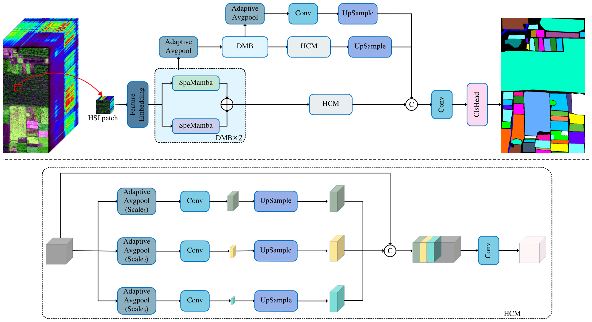
Figure 1 depicts the overall architecture of the proposed method, where an input HSI $\mathbf{H}\in {\mathbb{R}}^{C\times H\times W}$ is first reduced to ${\mathbf{H}}^{\prime }\in {\mathbb{R}}^{c\times H\times W}$ via PCA dimensionality reduction, and then divided into overlapping HSI patch cubes ${\{{\mathbf{x}}_i\in {\mathbb{R}}^{c\times w\times w}\}}_{i=1}^{H\times W}$, which are classified based on the central pixel. Here, C, H, and W denote, respectively, the number of spectral bands, height, and width of the original HSI; c is the reduced spectral dimension; and w represents the width and height of HSI cubes. The optimal values of c and w will be determined through parameter analysis in Section 4.3.

Given an input HSI patch $\mathbf{X}\in {\mathbb{R}}^{c\times w\times w}$, it is first mapped to an initial representation ${\mathbf{X}}_0$ via a feature embedding layer, which encodes the original spectral–spatial information into a higher-dimensional feature space. The resulting ${\mathbf{X}}_0$ is immediately fed into the first branch. Then introduce progressive downsampling via adaptive average pooling after the DMB output of this branch. This sequentially constructs the second and third branches, each with a lower spatial resolution than the previous one. A hierarchical multi-scale feature extraction architecture is thus established.

The first branch consists of two serially stacked DMBs and an HCM. Each DMB contains two parallel submodules, namely SpaMamba and SpeMamba (their detailed structures are described in Section 3.2 and are omitted here for brevity), which model the spatial and spectral dimensions of the input features, respectively. The outputs of the two branches are fused via element-wise addition to form the output of each DMB. The output of the k-th DMB is denoted as

$${\mathbf{F}}_{\mathrm{n}}^{\left(k\right)}=\mathrm{SpaMamba}\left({\mathbf{F}}_{\mathrm{n}}^{(k-1)}\right)+\mathrm{SpeMamba}\left({\mathbf{F}}_{\mathrm{n}}^{(k-1)}\right),k=1,2,$$

(1)

where ${\mathbf{F}}_1^{\left(0\right)}={\mathbf{X}}_0$ serves as the initial input for the first branch, and n indicates the n-th branch, with resolution decreasing from high to low. $\mathrm{SpaMamba}(·)$ and $\mathrm{SpeMamba}(·)$ denote the two parallel submodules responsible for modeling the spatial and spectral dimensions of the input features. The output of the first branch after two serial DMBs is denoted as ${\mathbf{F}}_1^{\left(2\right)}$. The output ${\mathbf{F}}_1^{\left(2\right)}$ is then fed into the HCM to aggregate multi-scale contextual information. The HCM adopts a strategy similar to pyramid pooling. It refines the input features at multiple distinct spatial scales.

Specifically, given the input feature map ${\mathbf{F}}_1^{\left(2\right)}$, the HCM first retains the original features as a base representation. In parallel, for each scale S in the predefined set $\mathrm{S}=\{{\mathrm{s}}_1,{\mathrm{s}}_2,{\mathrm{s}}_3\}$, the input features are spatially compressed via adaptive average pooling. This yields the global context specific to that scale:

$${\mathbf{P}}_{\mathrm{S}}={\mathrm{AdaptiveAvgpool}}_{\mathrm{S}}\left({\mathbf{F}}_1^{\left(2\right)}\right),$$

(2)

where ${\mathrm{AdaptiveAvgpool}}_{\mathrm{S}}(·)$ denotes the adaptive average pooling operation at three different scales and ${\mathbf{P}}_{\mathrm{S}}$ denotes the features obtained after adaptive average pooling at different sizes. Then, each pooled feature undergoes convolution for channel reduction and enhanced non-linear expressiveness. They are subsequently upsampled to the original resolution via bilinear interpolation, ensuring strict spatial alignment before fusion:

$${\mathbf{R}}_{\mathrm{S}}=\mathrm{UpSample}\left(\mathrm{Conv}\left({\mathbf{P}}_{\mathrm{S}}\right)\right),$$

(3)

where $\mathrm{Conv}(·)$ stands for the convolution operation, $\mathrm{UpSample}(·)$ corresponds to the bilinear upsampling, and ${\mathbf{R}}_{\mathrm{S}}$ indicates the features restored to the original spatial resolution.

Finally, the original high-resolution features and the multi-scale upsampled features are concatenated along the channel dimension. A convolutional fusion layer then compresses the concatenated features back to the original channel dimension. This produces the final output of the first branch:

$${\tilde{\mathbf{F}}}_1=\mathrm{Conv}\left(\mathrm{Concat}({\mathbf{F}}_1^{\left(2\right)},{\mathbf{R}}_{{\mathrm{s}}_1},{\mathbf{R}}_{{\mathrm{s}}_2},{\mathbf{R}}_{{\mathrm{s}}_3})\right)$$

(4)

The second branch retains a similar structural design as the first branch but stacks only a single DMB module. Its input likewise undergoes modeling along the spatial and spectral dimensions, as well as feature fusion, resulting in the output ${\tilde{\mathbf{F}}}_2$ of this branch.

Given the small HSI input patches, features fed into the third branch are already heavily downsampled. Because the receptive field is now broad enough to capture the global context, additional DMB and HCM modules become redundant. Unlike the preceding branches that integrate multiple DMBs and HCMs, the final branch adopts a relatively lightweight structure, simplified to just an Adaptive Avgpool, a convolution, and an upsampling layer to produce ${\tilde{\mathbf{F}}}_3$. This design reduces overhead while effectively completing the coarse-to-fine multi-scale representation.

Finally, to fully integrate the multi-scale contextual information, the outputs of the three branches, ${\tilde{\mathbf{F}}}_1$, ${\tilde{\mathbf{F}}}_2$, and ${\tilde{\mathbf{F}}}_3$, are concatenated along the channel dimension. The concatenated features are subsequently fused through a convolutional layer and fed into the classification head to generate the final prediction result $\mathbf{P}$, which can be expressed as the following equation:

$$\mathbf{P}=\mathrm{Cls}\left(\mathrm{Conv}\left(\mathrm{Concat}\left({\tilde{\mathbf{F}}}_1,{\tilde{\mathbf{F}}}_2,{\tilde{\mathbf{F}}}_3\right)\right)\right),$$

(5)

where $\mathrm{Concat}(·)$ denotes the concatenation operation along the channel dimension, $\mathrm{Conv}(·)$ represents the convolution operation, and $\mathrm{Cls}(·)$ refers to the classification head used to map feature into the prediction probabilities.

3.2. Dual Mamba Block

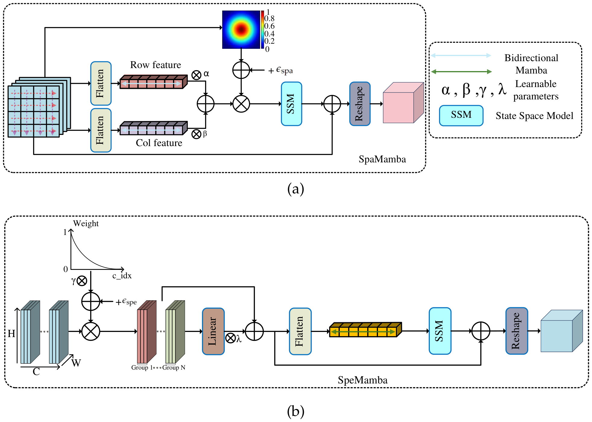
To fully exploit the inherent attributes of HS features, the DMB employs a parallel and decoupled feature extraction mechanism guided by physical priors. As illustrated in Figure 2, it consists of two independent submodules: SpaMamba and SpeMamba.

Specifically, to capture complex spatial contexts, SpaMamba introduces an adaptive Gaussian spatial prior with a base bias. This mechanism dynamically emphasizes the central pixel while preserving valid features from peripheral contexts.

Given the input feature map $\mathbf{F}$, to comprehensively model the spatial context, SpaMamba first flattens and processes the input along the row and column directions independently; feature extraction is expressed as

$${\mathbf{F}}_{\mathrm{row}}/\mathrm{col}={\mathrm{BMamba}}_{\mathrm{row}}/\mathrm{col}\left({\mathrm{Flatten}}_{\mathrm{row}}/\mathrm{col}\left(\mathbf{F}\right)\right),$$

(6)

where ${\mathrm{BMamba}}_{\mathrm{row}}/\mathrm{col}(·)$ is the bidirectional spatial Mamba [33] processors that perform selective scanning on 1D sequences. ${\mathbf{F}}_{\mathrm{row}}/\mathrm{col}$ represents the spatial feature maps processed along the row and column directions, and ${\mathrm{Flatten}}_{\mathrm{row}}/\mathrm{col}(·)$ denotes the operation that unfolds the 2D feature map into 1D sequences along the row and column directions. Subsequently, the two-directional representations are fused via a learnable weighted summation to adaptively balance their contributions:

$${\mathbf{F}}_{\mathrm{fspa}}=\alpha {\mathbf{F}}_{\mathrm{row}}+\beta {\mathbf{F}}_{\mathrm{col}},$$

(7)

where $\alpha$ and $\beta$ are learnable scalar weights normalized by the Softmax function, and ${\mathbf{F}}_{\mathrm{spa}}$ denotes the initially extracted spatial features. To ensure an unbiased initial contribution from both directions, $\alpha$ and $\beta$ are both initialized to 0.5. This uniform initialization ensures that the model is not prematurely biased toward any specific spatial direction during the early training stage. During the training phase, continuously fine-tuning these two parameters enables the network to adaptively capture directional features, thereby effectively improving the final classification performance.

Crucially, to emphasize the central target while preserving valid peripheral contexts, we construct an adaptive Gaussian spatial prior. For a pixel at spatial coordinates $(\mathrm{i},\mathrm{j})$, its squared Euclidean distance to the spatial center $({\mathrm{i}}_{\mathrm{c}},{\mathrm{j}}_{\mathrm{c}})$ is calculated as

$${\mathrm{d}}_{\mathrm{i},\mathrm{j}}={\left(\mathrm{i}-{\mathrm{i}}_{\mathrm{c}}\right)}^2+{\left(\mathrm{j}-{\mathrm{j}}_{\mathrm{c}}\right)}^2.$$

(8)

The Gaussian weight mask $\mathbf{M}$ is computed element-wise. For each spatial location $(\mathrm{i},\mathrm{j})$, its value ${\mathrm{M}}_{\mathrm{i},\mathrm{j}}$ is defined as

$${\mathrm{M}}_{\mathrm{i},\mathrm{j}}=exp(-\mathrm{softplus}\left(\theta \right){\mathrm{d}}_{\mathrm{i},\mathrm{j}}),\mathrm{softplus}(·)=ln(1+exp(·))$$

(9)

where $\theta$ is a learnable decay parameter. To ensure the physical validity of the Gaussian spatial prior during gradient updates, the $\mathrm{softplus}(·)$ function is employed to strictly constrain the effective decay rate to be positive. By equating this effective decay rate to the standard Gaussian function $exp(-{\displaystyle \frac{d^2}{2{\sigma }^2}})$, we establish that the equivalence $\mathrm{softplus}\left(\theta \right)$ is equivalent to ${\displaystyle \frac{1}{2{\sigma }^2}}$. Aiming to establish a physically meaningful receptive field from the start, the raw parameter $\theta$ is initialized to $1.0/(2\times {(w/3.0)}^2)$. This specific formulation is fundamentally motivated by the $3\sigma$ rule of the Gaussian distribution, seeking an ideal effective spread ($3\sigma =w$) that precisely aligns with the physical boundary of $w\times w$. During training, $\theta$ is dynamically updated, rendering the model highly robust and relatively insensitive to the exact initial values. This adaptive mask is then applied to the fused feature ${\mathbf{F}}_{\mathrm{fspa}}$ with an additional bias ${ϵ}_{\mathrm{spa}}$, formulated as

$${\mathbf{F}}_{\mathrm{Spa}}\_\mathrm{prior}={\mathbf{F}}_{\mathrm{fspa}}\otimes (\mathbf{M}+{ϵ}_{\mathrm{spa}}),$$

(10)

where ⊗ denotes element-wise multiplication. The baseline bias ${ϵ}_{\mathrm{spa}}$ acts as a soft constraint to prevent the complete attenuation of boundary features. A detailed discussion on the selection and sensitivity analysis of this parameter is provided in Section 4.3.

To yield the ultimate spatial representation, the prior-guided features ${\mathbf{F}}_{\mathrm{Spa}\_\mathrm{prior}}$ sequentially pass through an SSM module. Combined with a residual connection from the initial input $\mathbf{F}$, a reshape operation is applied to obtain the final output ${\mathbf{F}}_{\mathrm{spa}}$ of the SpaMamba submodule.

In parallel to SpaMamba, the SpeMamba submodule captures spectral dependencies using a PCA-inspired spectral decay prior with a base weight. Specifically, PCA computes the covariance matrix $\Sigma$ of the original HS data and performs eigenvalue decomposition:

$$\Sigma {\mathbf{v}}_{\mathrm{c}}={\lambda }_{\mathrm{c}}{\mathbf{v}}_{\mathrm{c}},{\lambda }_1\ge {\lambda }_2\ge \cdots \ge 0$$

(11)

where ${\lambda }_{\mathrm{c}}$ and ${\mathbf{v}}_{\mathrm{c}}$ denote the $\mathrm{d}$-th eigenvalue and its corresponding eigenvector, respectively. Since PCA arranges the principal components according to their explained variance, earlier principal components generally preserve more informative spectral characteristics than later ones. Inspired by this statistical property, we introduce a spectral decay prior as a physics-inspired inductive bias to guide subsequent feature learning. Let $\mathrm{y}\in \{0,1,\dots ,\mathrm{c}-1\}$ denote the channel index. To ensure stability, the indices are normalized to $[0,1]$. The spectral weight vector $\mathbf{w}$ is constructed as a smooth exponentially decaying prior along the channel dimension. Specifically, for the $\mathrm{k}$-th channel, its corresponding scalar weight ${\mathrm{w}}_{\mathrm{y}}$ is formulated as

$${\mathrm{w}}_{\mathrm{y}}=exp\left(-\gamma ·{\displaystyle \frac{\mathrm{y}}{\mathrm{c}-1}}\right),$$

(12)

where $\gamma$ is a learnable decay parameter, with its initial value set to 0.05. The purpose of this initialization is to provide a moderate and smoothly decaying exponential profile along the spectral dimension during the early stages of training. A large initial value may prematurely suppress spectral details that still contain informative cues. In contrast, a smaller initialization enables the model to focus on the dominant spectral components while retaining fine-grained spectral information. Aggregating these elements into the vector $\mathbf{w}$, the prior-guided feature is then obtained via channel-wise multiplication:

$${\mathbf{F}}_{\mathrm{Spe}\_\mathrm{prior}}=\mathbf{F}\otimes \left(\mathbf{w}+{ϵ}_{\mathrm{spe}}\right),$$

(13)

where ${ϵ}_{\mathrm{spe}}$ denotes the spectral baseline bias, introduced to prevent the over-suppression of trailing channels and preserve fine-grained spectral cues. A sensitivity analysis of this parameter is conducted in Section 4.3. It should be noted that the proposed spectral decay prior does not assume a strict one-to-one correspondence between the embedded feature channels and the original PCA components after the feature embedding layer. Instead, it serves as a physics-inspired inductive bias derived from the PCA variance distribution, encouraging the network to emphasize informative spectral representations during feature learning. Following the application of the spectral prior, the feature ${\mathbf{F}}_{\mathrm{Spe}\_\mathrm{prior}}$ is uniformly divided into $\mathrm{N}$ groups along the channel dimension. A linear layer is then applied to extract local spectral interactions within these groups, followed by multiplication with a learnable scaling factor $\lambda$. Combined with a residual connection, this intermediate feature ${\mathbf{F}}_{\mathrm{lin}}$ is formulated as:

$${\mathbf{F}}_{\mathrm{lin}}=\lambda ·\mathrm{Linear}\left({\mathbf{F}}_{\mathrm{Spe}\_\mathrm{prior}}\right)+{\mathbf{F}}_{\mathrm{Spe}\_\mathrm{prior}}.$$

(14)

We initialize $\lambda$ to a small positive value of 0.01. This design ensures that in the early stages of training, the network relies primarily on the prior-guided feature ${\mathbf{F}}_{\mathrm{Spe}\_\mathrm{prior}}$, while the contribution of the grouped linear interaction is introduced conservatively and gradually strengthens as $\lambda$ is optimized over the course of training. In few-shot scenarios with strong prior dependence, this amounts to letting the newly introduced learnable interaction branch intervene in a “gentle exploration” manner, preventing it from competing on equal footing with the carefully designed physics-based prior features from the outset. It thus balances training stability with the progressive enhancement of representational capacity.

To further establish global spectral dependencies, the intermediate feature ${\mathbf{F}}_{\mathrm{lin}}$ is flattened into a 1D sequence and processed by a $\mathrm{BMamba}$ block. This intermediate global representation is denoted as ${\mathbf{F}}_{\mathrm{Spe}\_\mathrm{global}}$

$${\mathbf{F}}_{\mathrm{Spe}\_\mathrm{global}}=\mathrm{BMamba}\left({\mathbf{F}}_{\mathrm{lin}}\right)$$

(15)

Adopting a symmetric refinement structure analogous to the spatial branch, the global spectral feature ${\mathbf{F}}_{\mathrm{Spe}\_\mathrm{global}}$ sequentially passes through an AdaptiveAvgpool layer and an SSM. Combined with a residual connection from the intermediate feature ${\mathbf{F}}_{\mathrm{lin}}$, a reshape operation is applied to obtain the final output ${\mathbf{F}}_{\mathrm{Spe}}$ of the SpeMamba submodule.

3.3. Feature-Level Contrastive Regularization

In FSL scenarios, standard CE loss often causes feature manifold collapse. While triplet [52] and center losses [53] mitigate this, they are hindered by inefficient pair construction and unstable center estimation. Thus, we introduce a feature-level contrastive regularizer to impose explicit topological constraints on the feature space.

Specifically, global pooling maps deep features into a vector $\mathbf{f}\in {\mathbb{R}}^d$. To eliminate numerical scaling and compact the feature manifold, $L_2$ normalization projects $\mathbf{f}$ onto the unit hypersphere ${\mathbb{S}}^{d-1}$, yielding $\mathbf{z}=\mathbf{f}/{\parallel \mathbf{f}\parallel }_2$. In this metric space, distances naturally translate to cosine similarities ${\mathbf{z}}_{\mathrm{i}}·{\mathbf{z}}_{\mathrm{j}}$. This regularizer explicitly enforces intra-class compactness and inter-class dispersion within a mini-batch, formulated as

$${\mathcal{L}}_{\mathrm{SupCon}}=\sum _{\mathrm{i}\in \mathrm{I}}{\displaystyle \frac{-1}{\left|\mathrm{P}\right(\mathrm{i}\left)\right|}}\sum _{\mathrm{p}\in \mathrm{P}\left(\mathrm{i}\right)}log{\displaystyle \frac{exp({\mathbf{z}}_{\mathrm{i}}·{\mathbf{z}}_{\mathrm{p}}/\tau )}{{\sum }_{\mathrm{a}\in \mathrm{A}\left(\mathrm{i}\right)}exp({\mathbf{z}}_{\mathrm{i}}·{\mathbf{z}}_{\mathrm{a}}/\tau )}}$$

(16)

where $\mathrm{I}$ denotes the set of indices for all samples in the current training batch, and $\mathrm{i}\in \mathrm{I}$ is the index of the anchor sample. $\mathrm{A}\left(\mathrm{i}\right)$ represents the set of all indices in the batch excluding the anchor $\mathrm{i}$ (i.e., $\mathrm{A}\left(\mathrm{i}\right)=\mathrm{I}\setminus \left\{\mathrm{i}\right\}$). $\mathrm{P}\left(\mathrm{i}\right)$ is the set of indices of all positive samples within $\mathrm{A}\left(\mathrm{i}\right)$ that share the same class label as the anchor $\mathrm{i}$, and $\left|\mathrm{P}\right(\mathrm{i}\left)\right|$ is its cardinality. $\tau$ is a scalar temperature parameter controlling the penalty strength on hard negatives. When $\tau$ is small, the exponential function $exp({\mathbf{z}}_{\mathrm{i}}·{\mathbf{z}}_{\mathrm{a}}/\tau )$ inside the denominator acts as a natural hard-negative miner. It assigns exponentially larger weights to negative samples that lie close to the anchor in the embedding space—so-called hard negatives. In our implementation, we set $\tau =0.07$ following standard contrastive learning practices. Because their exponentiated similarities completely dominate the denominator, the gradient updates automatically focus on repelling these most confusing samples. Known as implicit hard sample mining, this mechanism effectively remodels the feature space without the computationally expensive and tedious explicit pair construction required by traditional metric learning.

Finally, the network is jointly optimized via a weighted summation:

$${\mathcal{L}}_{\mathrm{total}}={\mathcal{L}}_{\mathrm{CE}}+\omega {\mathcal{L}}_{\mathrm{SupCon}}$$

(17)

where ${\mathcal{L}}_{\mathrm{CE}}$ is the standard CE loss applied to the final predicted logits, and $\omega$ is a weighting hyperparameter designed to balance the two optimization objectives. In our experiments, we empirically set $\omega =0.1$ to ensure that the auxiliary contrastive regularization maintains a comparable numerical scale with the cross-entropy loss, preventing it from dominating the primary classification task.

4. Experimental Section

This section presents datasets, experimental setup, and results. We begin by describing the benchmark datasets used in our experiments. Then we introduce the experimental setup, including performance metrics and experimental considerations detail. Subsequently, we conduct a comprehensive qualitative and quantitative analysis experiment with the proposed method and SOTA algorithm. Finally, a large number of ablation experiments are carried out to verify the effectiveness of our proposed methods.

4.1. Datasets

The experiments are carried out on three benchmark datasets, including HanChuan, HongHu, and XiongAn. The detailed descriptions of these datasets are provided as follows:

(A)

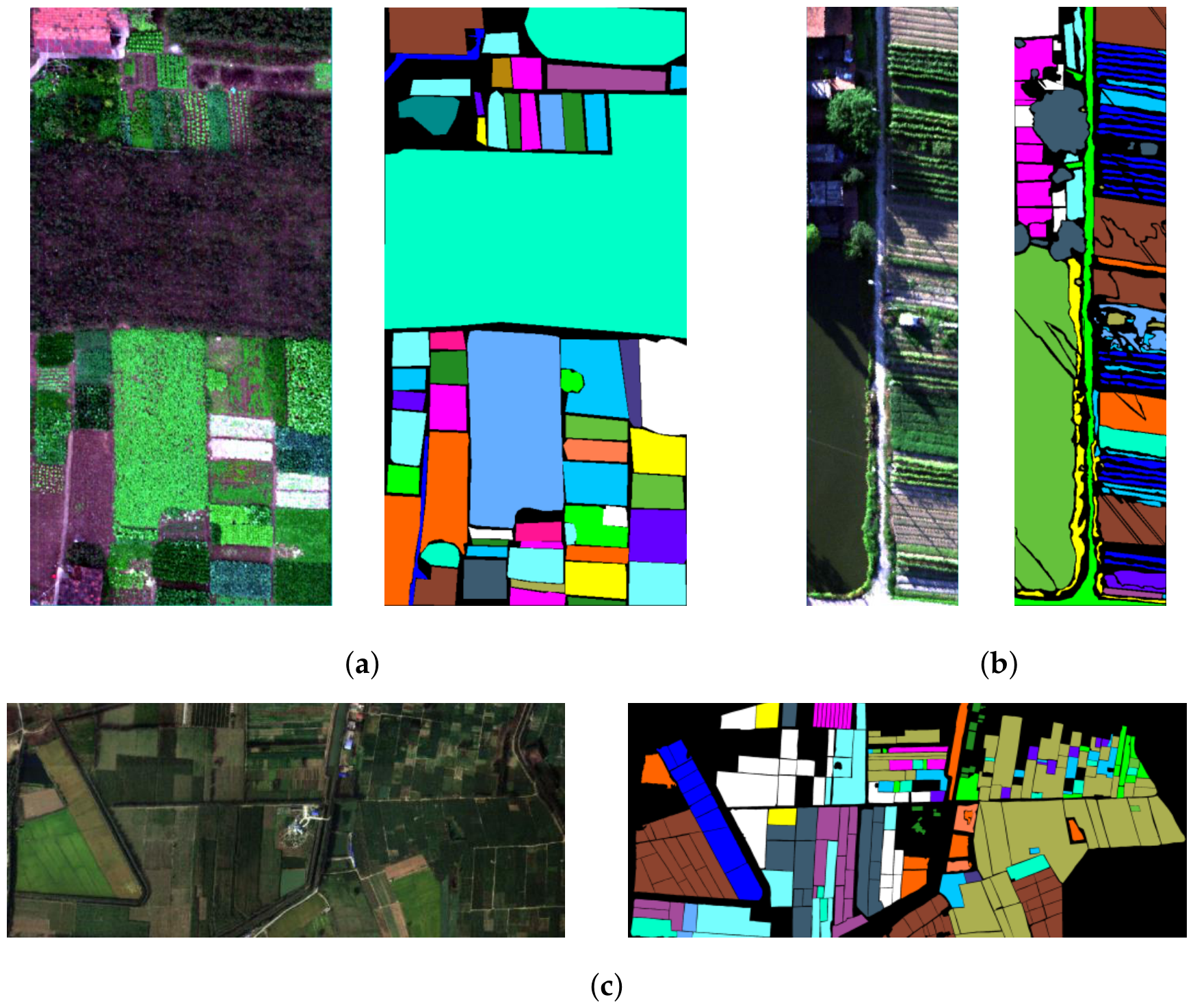
HongHu: The HongHu dataset is an HS scene collected over the Honghu area and is frequently adopted for HSI analysis tasks. The image covers an area of 940 × 475 pixels at a fine spatial resolution of 0.043 m. It contains 270 spectral channels ranging from 400 to 1000 nm and provides labeled samples for 22 different land-cover classes. A visual summary of the dataset is provided in Figure 3a, showing the original HSI and the corresponding ground truth.

(B)

HanChuan: HanChuan is a representative HS benchmark dataset acquired over Hanchuan City. The dataset provides an HSI of size 1217 × 303 pixels with a spatial resolution of 0.109 m. It consists of 274 spectral bands spanning the wavelength range from 400 to 1000 nm and includes ground-truth annotations for 16 land-cover categories. Figure 3b offers a visual overview of the dataset.

(C)

XiongAn: The XiongAn dataset comprises an HSI with a spatial size of 3750 × 1580 pixels. The image contains 250 spectral bands covering the 400–1000 nm wavelength range, with a spatial resolution of 0.5 m. The dataset includes 19 annotated land-cover classes, which are mainly composed of economic crops. A visual summary of the dataset, paired with its ground truth, is provided in Figure 3c.

To further explain the specific composition of the datasets,

Table 1. Sample distribution and color annotations of land-cover classes in HongHu, XiongAn, and HanChuan datasets.

No.	Color	HongHu		XiongAn		HanChuan
		Class	Numbers	Class	Numbers	Class	Numbers
1		Red roof	14,041	Swamp rice	26,138	Strawberry	44,735
2		Road	3512	Rice stubble	187,425	Cowpea	22,753
3		Bare soil	21,821	Water	124,862	Soybean	10,287
4		Cotton	163,285	Grassland	91,518	Sorghum	5353
5		Cotton firewood	6218	Willow	197,218	Water spinach	1200
6		Rape	44,557	Elm	19,663	Watermelon	4533
7		Chinese cabbage	24,103	Acer negundo	296,538	Greens	5903
8		Pakchoi	4054	Ash tree	276,755	Trees	17,978
9		Cabbage	10,819	Goldenrain tree	44,232	Grass	9469
10		Tuber mustard	12,394	Chinese scholar tree	372,708	Red roof	10,516
11		Brassica parachinensis	11,015	Peach tree	67,210	Gray roof	16,911
12		Brassica chinensis	8954	Vegetable garden	29,763	Plastic	3679
13		Small Brassica chinensis	22,507	Corn	85,547	Bare soil	9116
14		Lactuca sativa	7356	Poplar	68,885	Road	18,560
15		Celtuce	1002	Pear tree	986,139	Bright object	1136
16		Film covered lettuce	7262	Soybeans	7456	Water	75,401
17		Romaine lettuce	3010	Lotus leaf	27,178	/	/
18		Carrot	3217	Locust	6506	/	/
19		White radish	8712	Buildings	26,140	/	/
20		Garlic sprout	3486	/	/	/	/
21		Broad bean	1328	/	/	/	/
22		Tree	4040	/	/	/	/
Total			386,693		2,941,881		257,530

gives the number of categories of the three datasets, the corresponding relationship between the color and the ground object category, and the total number of samples in each dataset.

4.2. Experiment Setting

(A)

Evaluation metrics: In the experiments, all performance metrics are assessed on the test set. Three widely used evaluation indicators for HSI classification are adopted, including Overall Accuracy (OA), Average Accuracy (AA), and the Kappa coefficient [54]. For clarity of presentation in the subsequent tables, the values of OA and AA are expressed as percentages (%), and the Kappa coefficient is multiplied by 100.

(B)

Configuration: All experiments were conducted on a workstation equipped with four NVIDIA Tesla V100-SXM2-32GB GPUs0 and an Intel(R) Xeon(R) Gold 6230 CPU. The operating system was Ubuntu 22.04.4 LTS, and the deep learning framework was implemented using PyTorch 2.7.1 with CUDA 11.8.

(C)

Implementation details: To simulate an FSL scenario, exactly five labeled samples per class were randomly selected to construct the training set, while all remaining samples were reserved for testing. All experiments were independently conducted ten times using different random seeds (0–9) to mitigate the bias caused by this random selection, with the final results reported as mean ± standard deviation. The training process used the Adam optimizer with a learning rate of $1\times {10}^{-3}$ and was run for 100 epochs. Furthermore, a batch size of 64 was adopted for the effective optimization of Equation (16) under the 5-shot setting. In the HanChuan, XiongAn, and HongHu datasets, each class contains only 5 labeled samples, with the total training pools strictly limited to 80, 95, and 110 samples, respectively. With random sampling at a batch size of 64, the expected number of samples per class in a single mini-batch is approximately 4.00, 3.37, and 2.91, ensuring that most classes obtain 2 to 4 positive anchors per batch. Meanwhile, since each class contains a maximum of 5 samples, this batch size guarantees that any given sample will have at least 59 negative samples within the mini-batch. Furthermore, the SupCon loss effectively accommodates rare edge cases—where only a single sample from a class is drawn due to sampling fluctuations—enabling smooth training without triggering division-by-zero errors. Therefore, setting the batch size to 64 not only effectively prevents feature-space collapse but also avoids the irrationality of using a batch size larger than the total training set.

4.3. Parameter Analysis

In this subsection, we analyze four key parameters: the retained dimensions of PCA, the hard-coded parameter for the PCA-inspired spectral decay prior, the hard-coded parameter for the Gaussian spatial prior, and the input patch size. These parameters influence the preservation of spectral features, the strength of prior guidance, and the spatial receptive field. By investigating performance trends under various configurations, we aim to determine the optimal settings that balance classification accuracy and computational overhead.

(A)

The retained dimensions of PCA (c)

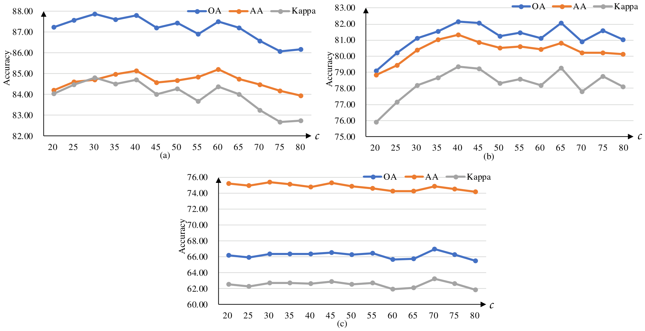
PCA dimensionality reduction aims to preserve the main discriminative spectral features in HS data, meanwhile eliminating redundant information and noise. With the size of input patch cubes fixed at $c\times 15\times 15$, we evaluated the impact of c (ranging from 20 to 80 with a step of 5) on model performance, and the experimental results are shown in Figure 4. It can be observed that on the HongHu and HanChuan datasets, the model performance improves steadily and approaches the optimum at 40 dimensions, while further increasing dimensions leads to a drop in accuracy. On the XiongAn dataset, the effect of PCA dimensions on performance is relatively slight and accuracy stays stable.

This observation suggests that the sensitivity of model performance to the number of retained PCA dimensions is highly data-dependent. When spectral bands exhibit redundancy, the choice of dimensionality becomes critical; conversely, when the spectral structure is inherently compact, the model exhibits stronger robustness to dimensional variation. In practice, for datasets like HongHu and HanChuan, where significant inter-band redundancy exists and discriminative information is distributed across numerous spectral channels, retaining too few dimensions forfeits critical information, while excessive retention introduces noise—hence the pronounced sensitivity to the PCA dimension. In contrast, for spectrally compact data such as XiongAn, where the majority of discriminative energy is concentrated in the first few principal components, performance remains stable as long as the retained dimension exceeds a certain minimum threshold; further increasing the dimensionality yields marginal additional information. This phenomenon is essentially attributable to the eigenvalue decay characteristics of the HSI covariance matrix.

(B)

The input patch size (w)

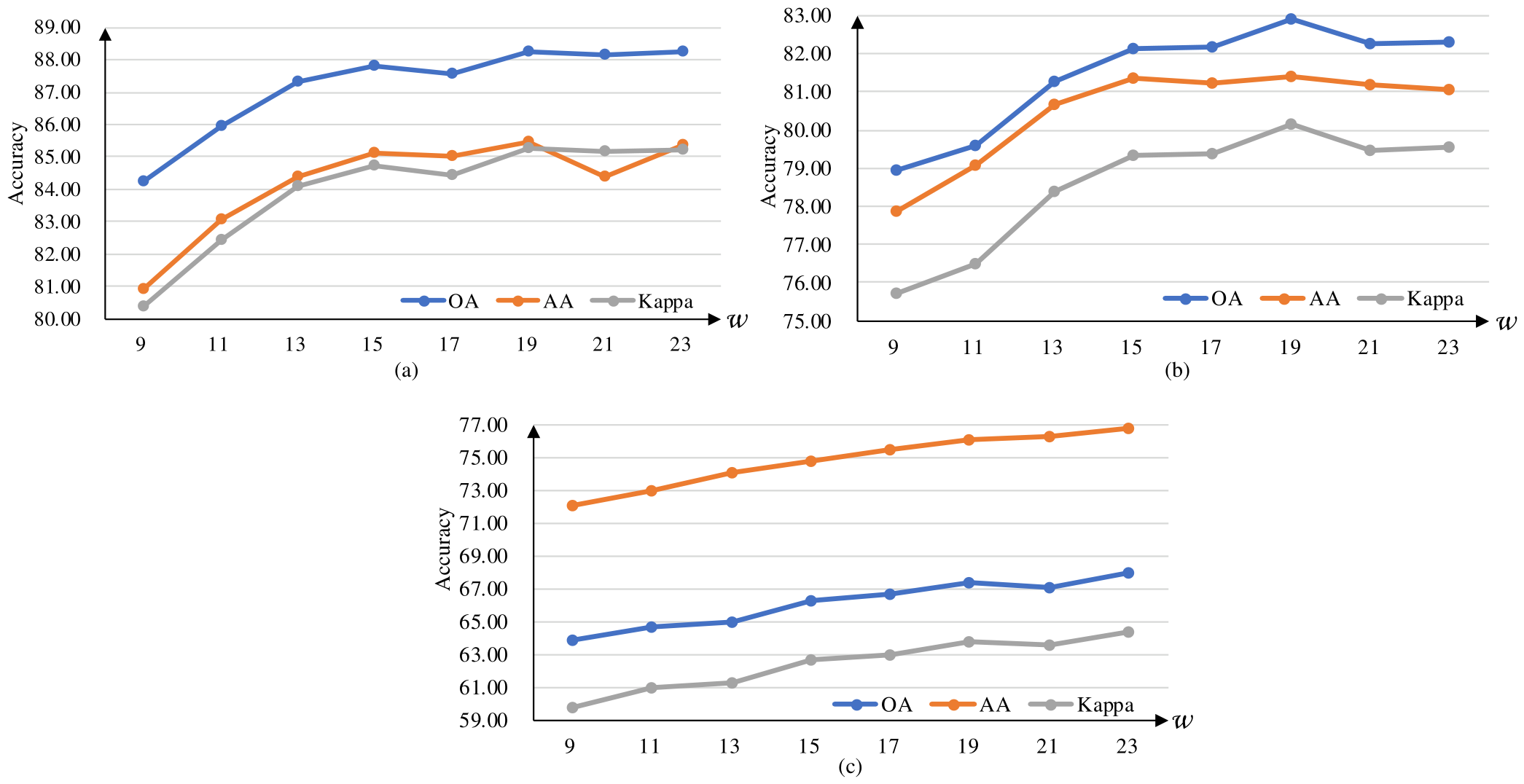
We investigated the effect of the size of input patch cubes w with the number of retained PCA dimensions c fixed at 40. A series of input patch sizes from $9\times 9$ to $23\times 23$ with a step of 2 are tested, and the results are shown in Figure 5. All patch sizes are odd to ensure that the central pixel is the target pixel. On the HongHu and HanChuan datasets, the classification performance exhibits an overall upward trend as the spatial context expands, peaking at $19\times 19$. Beyond this optimal size, the accuracy fluctuates and even degrades. This is because an excessively large receptive field introduces irrelevant background noise and heterogeneous pixels, which mislead the model, alongside a sharp rise in computational overhead. On the XiongAn dataset, accuracy rises continuously but much more slowly beyond $19\times 19$, along with excessive computational cost.

The spatial resolutions of HongHu and HanChuan are relatively high, at 0.043 m and 0.109 m, respectively. When w = 19, the receptive field fits neatly around the central pixel, capturing a purely homogeneous local context. But because agricultural plots in these scenes are often small and fragmented, enlarging the patch further tends to cross object boundaries and pull in a lot of heterogeneous pixels—background or other crop types. This inter-class interference dilutes the spectral purity of the target and severely misleads the model. In contrast, XiongAn has a coarser resolution of 0.5 m, and its crops are mostly distributed in large continuous blocks. Even when the patch size exceeds $19\times 19$, the receptive field still largely stays within the same class, so the accuracy continues to rise, albeit slowly. Still, this improvement comes with a sharp increase in computation, making the marginal return from further enlarging the patch rather limited.

(C)

The parameter for the PCA spectral prior (${ϵ}_{\mathrm{spe}}$)

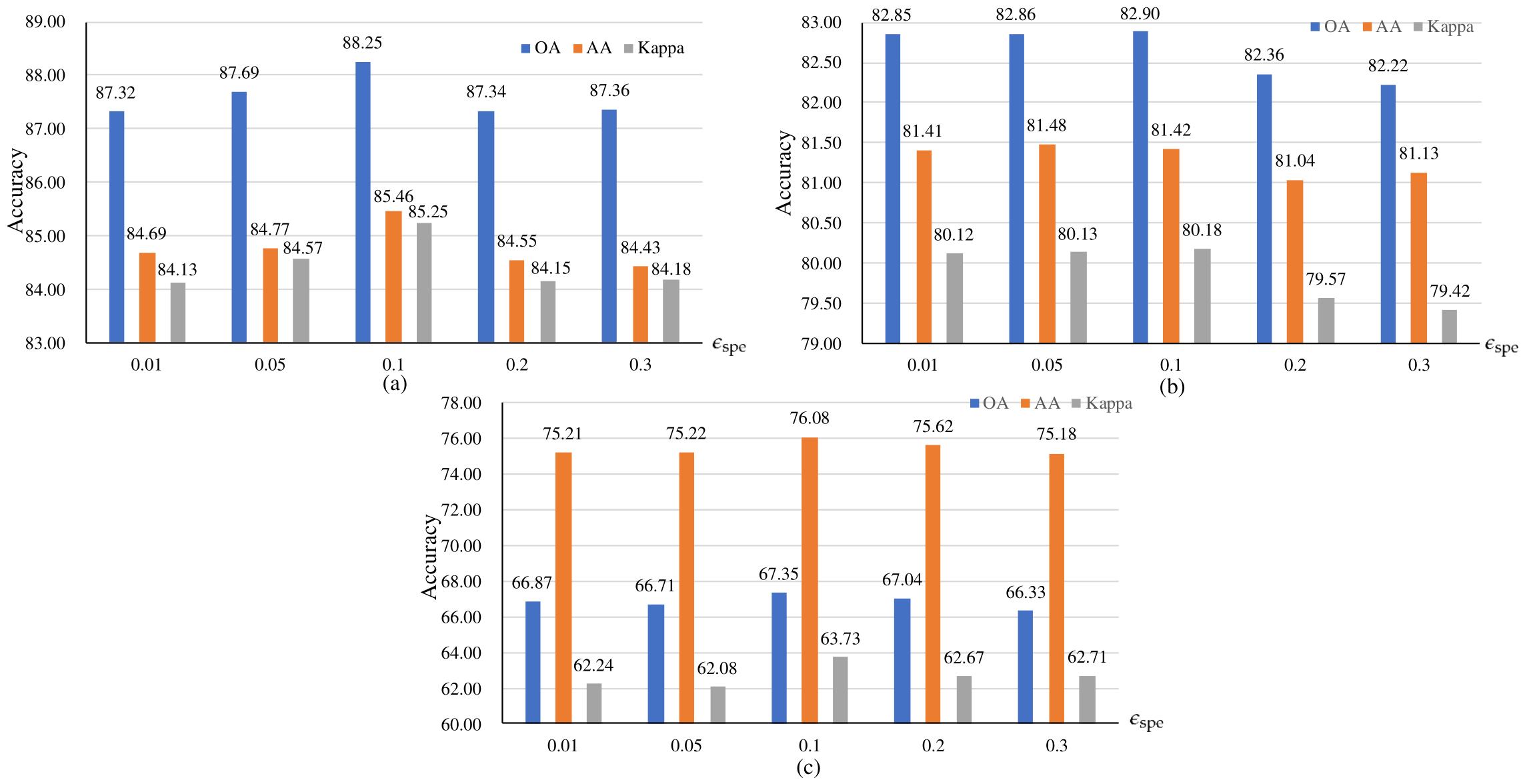
The baseline bias ${ϵ}_{\mathrm{spe}}$ in the PCA spectral prior serves to preserve valid discriminative information in low-energy channels, thereby preventing feature collapse under extreme five training samples condition. To evaluate its influence on model performance, we tested ${ϵ}_{\mathrm{spe}}$ over a range of candidate values—0.01, 0.05, 0.1, 0.2, and 0.3. Figure 6 presents the resulting OA, AA, and Kappa trends on the three datasets as ${ϵ}_{\mathrm{spe}}$ varies. On the three datasets, classification performance improves steadily as ${ϵ}_{\mathrm{spe}}$ increases from 0.01 to 0.1, peaking at the latter value. Further raising it to 0.2 or 0.3, however, leads to a noticeable decline in accuracy.

When ${ϵ}_{\mathrm{spe}}$ is set too small, like 0.01, the soft constraint imposed by the baseline bias becomes overly weak, which causes the network to over-suppress low-energy spectral channels. Although these tail channels account for only a small fraction of the overall variance, they may still carry fine-grained spectral cues that help distinguish similar crop types. Over-suppressing them therefore discards critical detail. Conversely, when ${ϵ}_{\mathrm{spe}}$ is too large—0.3, for instance—the baseline bias becomes excessively strong and substantially weakens the guiding effect of the PCA spectral decay prior. The network then loses its ability to focus on the most informative principal bands, and instead assigns excessive weight to redundant bands and spectral noise, which ultimately compromises the discriminability of the extracted features.

(D)

The parameter for the Gaussian spatial prior (${ϵ}_{\mathrm{spa}}$)

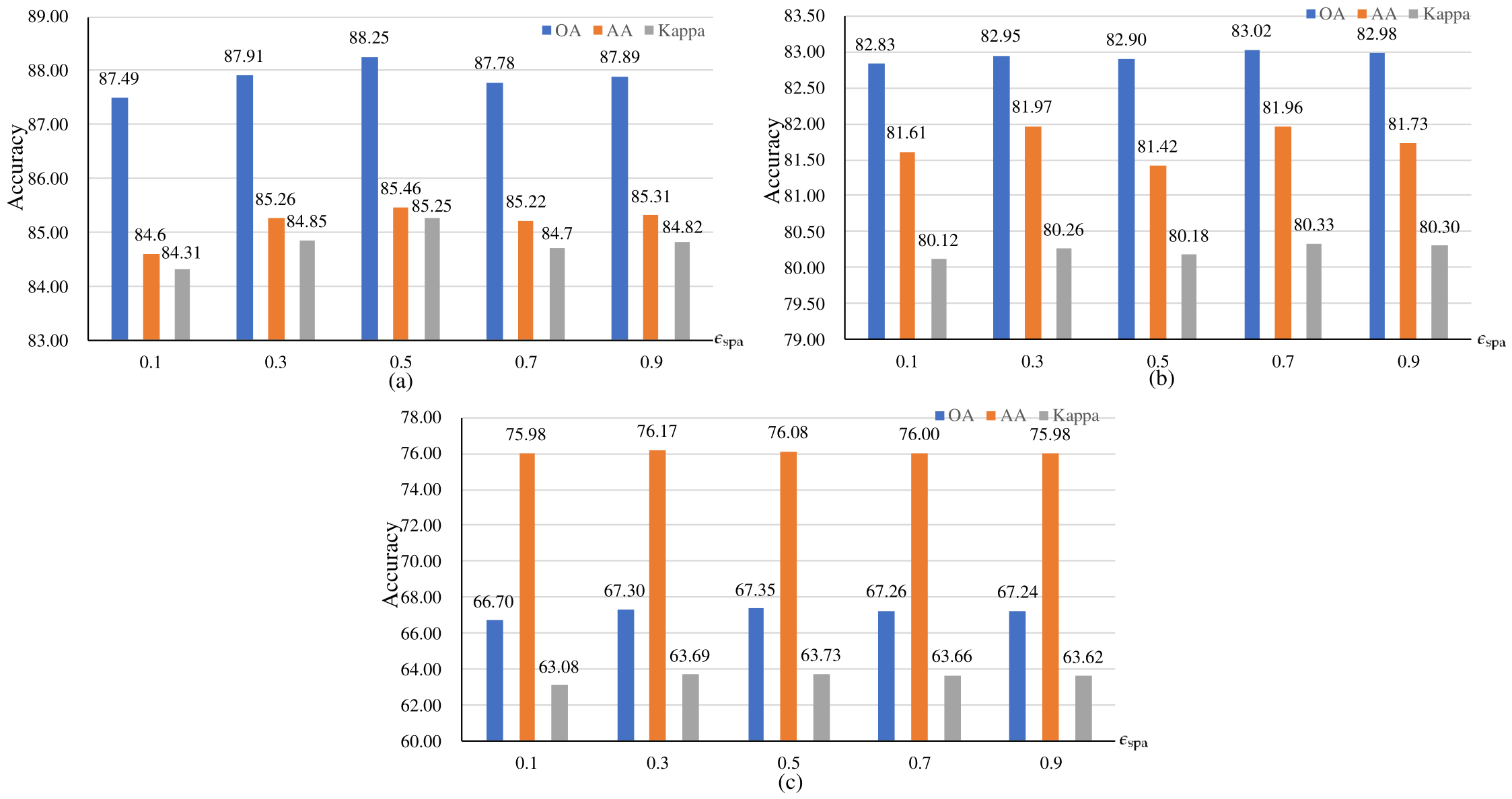
The baseline bias ${ϵ}_{\mathrm{spa}}$ in the Gaussian spatial prior is a soft constraint that prevents boundary features from being completely attenuated. To assess its impact on model performance, we tested ${ϵ}_{\mathrm{spa}}$ over candidate values ranging from 0.1 to 0.9 at intervals of 0.2. Figure 7 illustrates the resulting classification performance on the three datasets. The optimal choice of ${ϵ}_{\mathrm{spa}}$ varies slightly across datasets and evaluation metrics. On the HongHu dataset, the model attains its best performance across all metrics at ${ϵ}_{\mathrm{spa}}$ = 0.5. For HanChuan, OA reaches a local peak of 83.02% at 0.7, whereas AA is highest at 0.3. A similar pattern emerges on the XiongAn dataset: although OA and Kappa peak at 0.5, reaching 67.35% and 63.73, respectively, AA shows a slight preference for a smaller bias of 0.3, where it reaches 76.17%.

This performance fluctuation suggests that a smaller ${ϵ}_{\mathrm{spa}}$ enables the network to better capture fine-grained features of minority classes—which benefits Average Accuracy—yet it may over-suppress global spatial context. On the other hand, a larger ${ϵ}_{\mathrm{spa}}$ weakens the prior’s ability to focus on central targets because the baseline bias becomes too strong, introducing excessive heterogeneous background noise. Given that spatial heterogeneity and class imbalance vary across different agricultural scenes, the optimal trade-off point shifts accordingly.

Based on the above analysis, we fixed the network parameters for all subsequent main experiments to achieve the best overall classification performance across diverse and complex agricultural scenes: the PCA retained dimension c = 40, input patch size w = 19, spectral prior bias ${ϵ}_{\mathrm{spe}}$ = 0.1, and spatial prior bias ${ϵ}_{\mathrm{spa}}$ = 0.5. This parameter combination is a deliberate choice based on the principle of global optimal compromise. Take the selection of c and w as an example. Increasing c or w may improve accuracy only slightly. Yet the benefit is often offset by added noise and a sharp rise in computation. We therefore intentionally sacrifice such negligible accuracy gains in order to preserve the model’s clear efficiency advantage.

When setting the physical prior parameters ${ϵ}_{\mathrm{spe}}$ and ${ϵ}_{\mathrm{spa}}$, certain bias values, such as ${ϵ}_{\mathrm{spa}}$ = 0.7 on the HanChuan dataset, may achieve local peaks on a single dataset or a particular evaluation metric. In contrast, the combination of 0.1 and 0.5 maintains a consistently high and balanced performance across all three datasets and all metrics, including OA, AA, and Kappa. By forgoing marginal gains on individual datasets, we effectively avoid overfitting the hyperparameters to specific scenes, thereby ensuring strong cross-scene generalization and robustness under the five-training-samples condition.

4.4. Quantitative and Qualitative Analysis

To comprehensively evaluate the superiority and robustness of the proposed DPMSCH-Net under extreme five-shot conditions, we conduct extensive quantitative and qualitative comparisons against ten SOTA spatial–spectral classification methods. The selected baseline competitors encompass a diverse range of recent advanced architectures, which can be primarily categorized into four groups. Specifically, these consist of CNN-based methods (CSCANet [55], SSEFN [56]) alongside Transformer-based models (GSC-VIT [10], DSFormer [57]). Furthermore, the comparison includes Mamba-based networks (IGroupSS-Mamba [58], MambaHSI [36], MambaHSI+ [37]) as well as hybrid architectures (SCluster-Former [42], MCTGCL [43], HSI-MFormer [46]). To ensure a fair and consistent comparison, all baseline methods were evaluated under the 5-shot sampling protocol. To mitigate performance variations caused by the random selection of training samples, each model was independently trained and tested ten times using the same random seeds from 0 to 9. The final results are reported as the mean and standard deviation over these runs. This protocol improves the statistical reliability of the evaluation and provides a more objective basis for performance comparison. In the following subsections, the quantitative analysis provides a detailed numerical assessment based on standard evaluation metrics across different datasets, while the qualitative analysis offers a visual examination of the generated classification maps relative to the ground truth.

4.4.1. Quantitative Analysis

The quantitative classification results for the three benchmark datasets are summarized in

Table 2. Quantitative classification performance on the HongHu dataset, with all results reported as mean ± standard deviation and the best results in bold.

Class	CNN-Based Methods		Transformer-Based Methods		Mamba-Based Methods			Hybrid Architecture Methods			Ours
	CSCANet	SSEFN	GSC-VIT	DSFormer	MambaHSI+	MambaHSI	IGroupSS-Mamba	SCluster-Former	MCTGCL	HSI-MFormer
1	$76.33\pm 1.99$	$\mathbf{96.30}\pm \mathbf{2.31}$	$72.49\pm 11.63$	$81.08\pm 5.85$	$83.62\pm 10.09$	$80.70\pm 9.41$	$94.30\pm 1.74$	$72.06\pm 20.17$	$85.39\pm 6.03$	$94.93\pm 2.12$	$82.11\pm 8.53$
2	$55.48\pm 13.03$	$59.61\pm 7.59$	$73.70\pm 16.18$	$71.67\pm 10.17$	$76.10\pm 12.62$	$69.68\pm 12.41$	$80.52\pm 5.13$	$57.61\pm 19.15$	$76.77\pm 12.32$	$74.29\pm 4.70$	$\mathbf{84.82}\pm \mathbf{9.79}$
3	$88.96\pm 2.58$	$\mathbf{90.82}\pm \mathbf{3.82}$	$72.11\pm 17.99$	$79.74\pm 4.41$	$82.16\pm 6.71$	$82.12\pm 3.86$	$83.87\pm 3.08$	$53.45\pm 28.48$	$73.94\pm 15.31$	$88.44\pm 1.27$	$81.69\pm 3.14$
4	$79.09\pm 7.85$	$\mathbf{99.31}\pm \mathbf{0.17}$	$84.10\pm 7.38$	$90.41\pm 7.43$	$98.46\pm 1.53$	$84.81\pm 7.86$	$93.78\pm 1.45$	$85.08\pm 14.33$	$92.98\pm 2.84$	$93.97\pm 1.36$	$97.41\pm 1.41$
5	$87.62\pm 5.83$	$29.05\pm 7.55$	$69.79\pm 15.68$	$72.91\pm 8.89$	$71.16\pm 26.04$	$81.08\pm 8.98$	$82.84\pm 6.00$	$59.03\pm 14.09$	$81.84\pm 9.05$	$79.67\pm 3.00$	$\mathbf{95.31}\pm \mathbf{2.37}$
6	$73.20\pm 11.14$	$91.61\pm 3.24$	$78.53\pm 11.68$	$90.32\pm 3.39$	$91.12\pm 1.50$	$81.10\pm 6.47$	$91.01\pm 1.37$	$81.68\pm 12.52$	$\mathbf{92.41}\pm \mathbf{3.15}$	$89.50\pm 1.40$	$92.34\pm 1.08$
7	$19.30\pm 10.23$	$\mathbf{85.44}\pm \mathbf{3.82}$	$61.60\pm 8.94$	$49.32\pm 16.54$	$51.28\pm 10.32$	$56.18\pm 12.04$	$52.51\pm 0.97$	$38.49\pm 14.05$	$65.51\pm 3.65$	$52.29\pm 1.16$	$63.11\pm 8.90$
8	$39.40\pm 10.39$	$45.24\pm 8.99$	$32.10\pm 6.40$	$52.24\pm 6.34$	$53.44\pm 14.38$	$60.55\pm 13.03$	$34.57\pm 3.36$	$24.93\pm 12.12$	$54.26\pm 7.58$	$38.33\pm 3.44$	$\mathbf{77.98}\pm \mathbf{7.76}$
9	$92.87\pm 2.82$	$\mathbf{97.99}\pm \mathbf{1.10}$	$89.66\pm 4.94$	$93.85\pm 1.48$	$84.67\pm 7.56$	$82.24\pm 9.07$	$92.91\pm 0.65$	$74.96\pm 25.37$	$95.04\pm 2.29$	$92.77\pm 0.73$	$92.74\pm 4.23$
10	$40.71\pm 14.97$	$\mathbf{85.00}\pm \mathbf{9.27}$	$69.59\pm 7.08$	$54.26\pm 11.82$	$54.04\pm 8.73$	$59.22\pm 21.3$	$59.20\pm 5.88$	$57.33\pm 28.12$	$72.55\pm 10.29$	$60.21\pm 3.23$	$82.48\pm 4.44$
11	$18.50\pm 3.54$	$\mathbf{74.99}\pm \mathbf{6.95}$	$52.92\pm 12.32$	$43.19\pm 16.01$	$37.58\pm 14.55$	$52.47\pm 9.21$	$73.56\pm 4.14$	$67.17\pm 11.76$	$60.45\pm 7.36$	$68.24\pm 4.62$	$71.24\pm 9.72$
12	$38.46\pm 10.32$	$57.32\pm 9.37$	$53.74\pm 18.06$	$50.31\pm 8.74$	$66.32\pm 8.93$	$58.68\pm 17.88$	$64.03\pm 2.29$	$55.05\pm 17.17$	$59.80\pm 8.79$	$57.77\pm 3.94$	$\mathbf{67.34}\pm \mathbf{13.76}$
13	$45.07\pm 10.20$	$\mathbf{77.78}\pm \mathbf{4.08}$	$48.91\pm 12.22$	$54.37\pm 16.17$	$67.02\pm 8.61$	$69.57\pm 3.73$	$56.52\pm 5.13$	$47.81\pm 25.62$	$49.17\pm 12.00$	$62.55\pm 3.51$	$63.84\pm 5.71$
14	$63.93\pm 10.99$	$79.32\pm 9.14$	$75.79\pm 14.51$	$61.46\pm 15.53$	$74.05\pm 13.00$	$67.03\pm 12.94$	$77.27\pm 6.40$	$52.59\pm 19.60$	$83.99\pm 9.06$	$81.84\pm 2.75$	$\mathbf{88.49}\pm \mathbf{9.56}$
15	$97.90\pm 2.27$	$44.62\pm 7.23$	$93.79\pm 3.47$	$97.70\pm 1.04$	$88.20\pm 8.25$	$95.17\pm 3.11$	$91.43\pm 2.03$	$78.92\pm 12.59$	$97.22\pm 1.43$	$93.11\pm 1.12$	$\mathbf{99.03}\pm \mathbf{1.26}$
16	$73.59\pm 10.73$	$94.16\pm 3.66$	$78.14\pm 10.76$	$85.36\pm 3.98$	$74.14\pm 11.07$	$75.5\pm 15.12$	$84.19\pm 2.79$	$85.17\pm 11.59$	$89.62\pm 4.42$	$87.05\pm 1.98$	$\mathbf{96.84}\pm \mathbf{1.89}$
17	$82.22\pm 27.65$	$62.66\pm 10.31$	$70.61\pm 14.95$	$61.94\pm 17.85$	$71.14\pm 15.35$	$71.91\pm 11.58$	$65.70\pm 15.73$	$43.86\pm 27.34$	$\mathbf{85.31}\pm \mathbf{10.88}$	$73.93\pm 17.51$	$83.53\pm 12.11$
18	$\mathbf{95.52}\pm \mathbf{4.34}$	$56.21\pm 11.08$	$72.77\pm 14.37$	$92.37\pm 4.99$	$78.61\pm 7.42$	$87.33\pm 4.54$	$91.11\pm 5.68$	$80.26\pm 17.82$	$94.77\pm 7.30$	$95.31\pm 1.41$	$93.84\pm 6.45$
19	$73.43\pm 6.47$	$78.09\pm 5.16$	$71.57\pm 13.98$	$83.74\pm 7.38$	$59.00\pm 19.28$	$75.16\pm 7.61$	$82.96\pm 4.48$	$60.02\pm 21.80$	$83.64\pm 8.19$	$80.62\pm 3.30$	$\mathbf{89.41}\pm \mathbf{6.78}$
20	$34.11\pm 7.53$	$67.53\pm 7.56$	$84.04\pm 16.28$	$90.25\pm 2.26$	$89.87\pm 17.10$	$91.09\pm 12.90$	$82.95\pm 4.15$	$\mathbf{95.36}\pm \mathbf{1.86}$	$86.54\pm 6.52$	$80.53\pm 2.48$	$87.45\pm 16.93$
21	$86.36\pm 6.65$	$33.94\pm 6.70$	$72.08\pm 26.79$	$72.23\pm 11.28$	$67.20\pm 21.06$	$93.36\pm 7.37$	$95.52\pm 2.96$	$87.88\pm 10.19$	$88.18\pm 11.17$	$\mathbf{97.26}\pm \mathbf{2.52}$	$96.95\pm 3.42$
22	$58.58\pm 11.27$	$32.67\pm 6.75$	$84.78\pm 9.69$	$91.20\pm 3.87$	$68.56\pm 15.24$	$87.16\pm 7.06$	$77.13\pm 3.31$	$62.25\pm 27.24$	$84.23\pm 12.75$	$84.79\pm 3.43$	$\mathbf{92.24}\pm \mathbf{10.05}$
OA	$68.26\pm 4.17$	$83.07\pm 2.22$	$75.38\pm 3.71$	$79.58\pm 3.13$	$83.28\pm 1.88$	$77.87\pm 4.23$	$83.21\pm 1.95$	$71.99\pm 8.88$	$79.71\pm 1.96$	$84.04\pm 0.91$	$\mathbf{88.25}\pm \mathbf{0.94}$
AA	$64.57\pm 1.61$	$69.98\pm 1.20$	$71.04\pm 2.90$	$73.63\pm 2.59$	$72.17\pm 3.41$	$75.55\pm 3.52$	$77.59\pm 1.03$	$64.59\pm 6.18$	$83.64\pm 1.23$	$78.50\pm 1.24$	$\mathbf{85.46}\pm \mathbf{1.34}$
Kappa	$61.66\pm 4.49$	$79.17\pm 2.53$	$70.05\pm 4.08$	$74.77\pm 3.49$	$70.38\pm 4.16$	$74.05\pm 3.09$	$79.14\pm 2.22$	$66.04\pm 9.34$	$79.63\pm 1.46$	$80.11\pm 1.08$	$\mathbf{85.26}\pm \mathbf{1.17}$

,

Table 3. Quantitative classification performance on the HanChuan dataset, with all results reported as mean ± standard deviation and the best results in bold.

Class	CNN-Based Methods		Transformer-Based Methods		Mamba-Based Methods			Hybrid Architecture Methods			Ours
	CSCANet	SSEFN	GSC-VIT	DSFormer	MambaHSI+	MambaHSI	IGroupSS-Mamba	SCluster-Former	MCTGCL	HSI-MFormer
1	$63.47\pm 8.51$	$\mathbf{92.76}\pm \mathbf{3.44}$	$69.35\pm 8.54$	$75.21\pm 5.20$	$80.07\pm 9.84$	$70.57\pm 10.19$	$86.75\pm 6.54$	$69.69\pm 14.23$	$78.41\pm 5.99$	$89.40\pm 2.87$	$84.35\pm 9.17$
2	$70.48\pm 7.39$	$\mathbf{92.95}\pm \mathbf{3.30}$	$41.75\pm 17.62$	$57.00\pm 8.75$	$64.39\pm 8.17$	$43.81\pm 9.26$	$53.43\pm 4.50$	$57.14\pm 11.61$	$67.40\pm 8.18$	$48.25\pm 3.00$	$70.65\pm 13.43$
3	$66.54\pm 16.34$	$70.65\pm 8.45$	$64.18\pm 18.87$	$68.74\pm 13.89$	$78.33\pm 15.33$	$74.67\pm 15.30$	$85.07\pm 3.39$	$68.43\pm 16.32$	$85.16\pm 11.65$	$\mathbf{88.46}\pm \mathbf{1.36}$	$82.82\pm 8.81$
4	$97.66\pm 1.09$	$71.99\pm 10.96$	$90.08\pm 3.72$	$95.91\pm 1.13$	$96.18\pm 2.37$	$94.05\pm 2.29$	$96.89\pm 0.56$	$92.42\pm 5.32$	$96.78\pm 1.71$	$97.52\pm 0.50$	$\mathbf{98.79}\pm \mathbf{1.06}$
5	$92.34\pm 7.54$	$26.59\pm 9.04$	$82.82\pm 17.61$	$95.93\pm 4.95$	$94.66\pm 7.02$	$96.42\pm 3.09$	$95.16\pm 1.06$	$\mathbf{97.15}\pm \mathbf{3.28}$	$95.04\pm 6.35$	$94.83\pm 1.76$	$96.03\pm 4.30$
6	$50.43\pm 5.26$	$44.93\pm 12.98$	$29.38\pm 13.86$	$39.38\pm 9.98$	$53.65\pm 6.18$	$41.28\pm 6.05$	$59.60\pm 7.12$	$45.01\pm 13.60$	$63.66\pm 9.37$	$67.28\pm 2.88$	$\mathbf{75.31}\pm \mathbf{9.16}$
7	$\mathbf{97.69}\pm \mathbf{0.98}$	$45.23\pm 10.35$	$74.74\pm 25.51$	$86.16\pm 8.71$	$88.47\pm 8.90$	$78.39\pm 17.73$	$90.55\pm 2.89$	$67.87\pm 19.61$	$81.56\pm 10.22$	$92.55\pm 1.90$	$93.01\pm 4.52$
8	$21.86\pm 11.04$	$\mathbf{90.33}\pm \mathbf{6.02}$	$25.76\pm 15.10$	$37.81\pm 12.78$	$54.64\pm 9.57$	$37.25\pm 9.14$	$48.21\pm 3.93$	$58.82\pm 9.35$	$55.94\pm 7.98$	$50.77\pm 2.57$	$63.33\pm 3.17$
9	$48.97\pm 14.08$	$68.62\pm 10.69$	$29.69\pm 15.42$	$41.46\pm 8.12$	$54.51\pm 10.63$	$48.28\pm 15.14$	$63.98\pm 2.42$	$55.66\pm 5.73$	$\mathbf{69.67}\pm \mathbf{7.28}$	$64.92\pm 2.22$	$68.24\pm 14.39$
10	$95.69\pm 2.20$	$83.06\pm 12.49$	$70.67\pm 23.01$	$84.94\pm 12.97$	$77.91\pm 16.58$	$72.07\pm 16.44$	$97.46\pm 0.72$	$58.52\pm 23.33$	$88.48\pm 17.71$	$\mathbf{97.97}\pm \mathbf{0.38}$	$91.33\pm 14.43$
11	$65.71\pm 10.87$	$58.73\pm 10.65$	$67.43\pm 17.43$	$67.83\pm 13.85$	$77.32\pm 15.88$	$66.01\pm 16.27$	$87.50\pm 3.95$	$46.65\pm 17.01$	$77.45\pm 11.46$	$\mathbf{89.02}\pm \mathbf{3.92}$	$84.30\pm 10.69$
12	$60.99\pm 15.17$	$37.45\pm 14.62$	$45.94\pm 17.59$	$60.21\pm 16.13$	$73.96\pm 12.11$	$63.04\pm 18.55$	$61.09\pm 3.57$	$62.96\pm 8.08$	$77.57\pm 9.42$	$55.72\pm 1.56$	$\mathbf{89.63}\pm \mathbf{10.82}$
13	$20.70\pm 9.11$	$41.96\pm 9.55$	$37.11\pm 18.96$	$53.28\pm 7.75$	$\mathbf{59.56}\pm \mathbf{5.45}$	$51.87\pm 8.50$	$43.74\pm 5.19$	$30.85\pm 18.86$	$52.37\pm 12.79$	$47.97\pm 4.13$	$51.92\pm 8.42$
14	$65.13\pm 10.28$	$\mathbf{80.80}\pm \mathbf{10.26}$	$55.27\pm 20.73$	$34.03\pm 11.34$	$76.06\pm 6.03$	$52.63\pm 12.55$	$67.67\pm 5.67$	$58.82\pm 13.97$	$57.84\pm 13.77$	$71.76\pm 4.39$	$70.35\pm 7.23$
15	$79.54\pm 6.46$	$45.23\pm 19.18$	$78.84\pm 12.07$	$80.03\pm 10.40$	$80.03\pm 11.39$	$76.15\pm 14.72$	$80.54\pm 4.51$	$75.92\pm 3.25$	$81.29\pm 16.69$	$77.09\pm 3.62$	$\mathbf{84.73}\pm \mathbf{9.24}$
16	$90.74\pm 5.35$	$\mathbf{98.36}\pm \mathbf{1.96}$	$83.47\pm 12.11$	$83.29\pm 19.88$	$94.34\pm 7.38$	$91.04\pm 10.08$	$87.10\pm 7.86$	$69.47\pm 24.70$	$90.92\pm 9.92$	$83.71\pm 5.11$	$94.79\pm 7.21$
OA	$70.26\pm 1.52$	$76.73\pm 3.11$	$63.73\pm 4.55$	$67.98\pm 6.13$	$78.84\pm 2.67$	$69.21\pm 3.93$	$77.45\pm 2.47$	$63.12\pm 8.09$	$76.22\pm 2.89$	$77.39\pm 1.72$	$\mathbf{82.90}\pm \mathbf{2.48}$
AA	$68.00\pm 1.94$	$65.60\pm 1.81$	$59.15\pm 3.12$	$66.33\pm 2.11$	$75.25\pm 1.81$	$66.1\pm 2.53$	$75.16\pm 0.79$	$63.46\pm 3.67$	$77.70\pm 2.81$	$76.07\pm 0.85$	$\mathbf{81.42}\pm \mathbf{1.81}$
Kappa	$65.83\pm 1.64$	$73.14\pm 3.46$	$58.56\pm 4.82$	$63.48\pm 6.27$	$74.53\pm 3.89$	$65.67\pm 5.52$	$74.09\pm 2.64$	$58.61\pm 8.02$	$74.27\pm 3.07$	$74.06\pm 1.87$	$\mathbf{80.18}\pm \mathbf{2.79}$

and

Table 4. Quantitative classification performance on the XiongAn dataset, with all results reported as mean ± standard deviation and the best results in bold.

Class	CNN-Based Methods		Transformer-Based Methods		Mamba-Based Methods			Hybrid Architecture Methods			Ours
	CSCANet	SSEFN	GSC-VIT	DSFormer	MambaHSI+	MambaHSI	IGroupSS-Mamba	SCluster-Former	MCTGCL	HSI-MFormer
1	$93.43\pm 4.49$	$\mathbf{99.21}\pm \mathbf{0.68}$	$89.37\pm 4.61$	$92.79\pm 3.14$	$83.37\pm 6.24$	$83.97\pm 8.67$	$91.54\pm 9.32$	$89.30\pm 10.00$	$92.28\pm 9.22$	$86.71\pm 9.88$	$95.31\pm 5.26$
2	$89.31\pm 5.35$	$\mathbf{94.50}\pm \mathbf{3.57}$	$86.29\pm 7.87$	$88.52\pm 5.49$	$89.37\pm 5.61$	$81.95\pm 7.73$	$85.94\pm 6.15$	$87.79\pm 6.46$	$87.89\pm 5.53$	$86.61\pm 5.64$	$89.17\pm 6.24$
3	$79.77\pm 11.25$	$94.61\pm 4.84$	$91.29\pm 7.88$	$\mathbf{95.43}\pm \mathbf{4.10}$	$91.13\pm 4.65$	$89.09\pm 9.88$	$85.00\pm 7.82$	$85.85\pm 15.74$	$87.45\pm 9.24$	$63.90\pm 11.53$	$91.85\pm 3.36$
4	$66.27\pm 9.74$	$45.61\pm 7.72$	$47.36\pm 21.09$	$53.57\pm 17.66$	$51.82\pm 13.90$	$42.88\pm 13.79$	$61.80\pm 11.81$	$57.13\pm 9.56$	$63.08\pm 12.50$	$\mathbf{70.54}\pm \mathbf{6.27}$	$67.82\pm 8.81$
5	$66.60\pm 6.07$	$70.69\pm 9.18$	$38.95\pm 12.01$	$37.41\pm 11.16$	$54.16\pm 6.47$	$53.26\pm 9.97$	$66.03\pm 8.04$	$52.64\pm 15.74$	$67.74\pm 8.41$	$\mathbf{91.56}\pm \mathbf{4.75}$	$75.47\pm 5.87$
6	$94.00\pm 3.09$	$22.33\pm 5.95$	$82.40\pm 5.96$	$90.19\pm 2.92$	$82.99\pm 6.08$	$83.69\pm 7.43$	$91.73\pm 5.81$	$91.55\pm 7.66$	$90.69\pm 5.95$	$49.71\pm 9.11$	$\mathbf{94.47}\pm \mathbf{3.17}$
7	$42.41\pm 12.55$	$\mathbf{66.14}\pm \mathbf{11.11}$	$36.25\pm 10.60$	$31.31\pm 6.41$	$38.20\pm 11.85$	$39.13\pm 9.65$	$46.93\pm 9.62$	$38.14\pm 12.15$	$49.34\pm 8.12$	$56.46\pm 16.53$	$55.53\pm 8.73$
8	$62.74\pm 9.15$	$58.95\pm 5.23$	$37.86\pm 7.40$	$31.39\pm 9.48$	$45.35\pm 16.97$	$45.79\pm 16.5$	$53.16\pm 11.86$	$44.73\pm 14.19$	$55.97\pm 12.23$	$\mathbf{86.13}\pm \mathbf{6.47}$	$61.03\pm 17.33$
9	$75.36\pm 7.94$	$53.76\pm 18.99$	$59.13\pm 6.14$	$58.58\pm 12.23$	$66.87\pm 13.12$	$67.14\pm 6.44$	$86.94\pm 4.40$	$83.89\pm 10.54$	$87.11\pm 6.01$	$50.64\pm 9.55$	$\mathbf{90.65}\pm \mathbf{6.94}$
10	$39.59\pm 9.92$	$66.83\pm 8.24$	$30.12\pm 9.00$	$14.78\pm 4.11$	$29.49\pm 12.79$	$26.99\pm 8.55$	$48.94\pm 9.52$	$47.54\pm 13.20$	$42.84\pm 9.16$	$\mathbf{73.15}\pm \mathbf{7.59}$	$54.90\pm 9.89$
11	$64.83\pm 15.53$	$48.92\pm 8.78$	$44.70\pm 13.60$	$39.09\pm 19.34$	$49.33\pm 9.97$	$43.19\pm 10.67$	$69.91\pm 7.23$	$73.12\pm 9.47$	$72.94\pm 7.21$	$57.92\pm 7.69$	$\mathbf{78.87}\pm \mathbf{8.73}$
12	$45.18\pm 8.95$	$18.29\pm 5.03$	$44.27\pm 10.15$	$44.95\pm 9.68$	$46.03\pm 8.70$	$47.45\pm 13.56$	$58.47\pm 7.24$	$66.98\pm 12.70$	$56.33\pm 9.21$	$40.93\pm 11.57$	$\mathbf{73.59}\pm \mathbf{6.76}$
13	$34.18\pm 10.64$	$26.10\pm 11.03$	$31.14\pm 7.28$	$23.21\pm 10.20$	$25.47\pm 8.56$	$28.78\pm 8.69$	$39.56\pm 10.52$	$39.32\pm 11.15$	$39.06\pm 9.98$	$\mathbf{63.95}\pm \mathbf{15.08}$	$47.85\pm 10.00$
14	$57.78\pm 12.01$	$33.99\pm 9.81$	$53.01\pm 11.66$	$64.88\pm 12.23$	$39.43\pm 12.42$	$33.71\pm 8.61$	$59.80\pm 15.70$	$\mathbf{87.39}\pm \mathbf{13.84}$	$59.20\pm 16.75$	$48.96\pm 6.31$	$68.46\pm 10.18$
15	$42.93\pm 6.44$	$\mathbf{88.20}\pm \mathbf{6.03}$	$25.13\pm 13.00$	$34.66\pm 12.81$	$39.59\pm 10.84$	$36.35\pm 8.13$	$48.15\pm 7.59$	$36.61\pm 15.89$	$44.17\pm 9.03$	$48.62\pm 12.45$	$54.07\pm 4.71$
16	$68.73\pm 12.30$	$30.48\pm 7.16$	$54.02\pm 12.49$	$61.49\pm 14.99$	$67.51\pm 11.32$	$69.05\pm 12.3$	$67.47\pm 9.63$	$66.30\pm 14.12$	$71.00\pm 11.83$	$68.62\pm 14.30$	$\mathbf{77.56}\pm \mathbf{11.98}$
17	$88.60\pm 10.41$	$30.48\pm 7.16$	$70.22\pm 13.31$	$70.27\pm 12.06$	$72.07\pm 12.84$	$76.09\pm 16.55$	$86.40\pm 9.36$	$88.68\pm 12.58$	$84.88\pm 12.14$	$89.83\pm 8.76$	$\mathbf{92.09}\pm \mathbf{8.76}$
18	$81.18\pm 28.52$	$32.20\pm 9.42$	$61.21\pm 8.95$	$54.68\pm 16.69$	$65.76\pm 14.18$	$83.68\pm 11.19$	$77.90\pm 18.56$	$81.19\pm 14.57$	$82.97\pm 13.49$	$81.57\pm 16.68$	$\mathbf{91.57}\pm \mathbf{12.33}$
19	$50.90\pm 13.40$	$76.81\pm 12.99$	$69.52\pm 11.00$	$\mathbf{85.33}\pm \mathbf{7.73}$	$78.08\pm 6.72$	$76.86\pm 8.89$	$67.12\pm 10.35$	$80.93\pm 12.84$	$84.02\pm 5.47$	$62.42\pm 13.24$	$85.27\pm 8.99$
OA	$58.44\pm 2.17$	$60.33\pm 2.44$	$46.18\pm 4.58$	$47.20\pm 4.40$	$51.60\pm 3.86$	$49.59\pm 3.35$	$60.88\pm 3.04$	$54.95\pm 5.05$	$60.05\pm 3.37$	$61.70\pm 2.54$	$\mathbf{67.35}\pm \mathbf{1.96}$
AA	$65.46\pm 3.27$	$52.97\pm 1.95$	$55.38\pm 2.01$	$56.45\pm 2.65$	$58.75\pm 2.29$	$58.37\pm 2.44$	$68.04\pm 2.05$	$66.80\pm 3.26$	$69.42\pm 1.55$	$69.12\pm 1.35$	$\mathbf{76.08}\pm \mathbf{0.90}$
Kappa	$54.24\pm 2.22$	$56.27\pm 2.34$	$41.76\pm 4.12$	$42.41\pm 3.93$	$46.4\pm 3.71$	$56.22\pm 3.48$	$56.78\pm 3.05$	$50.81\pm 4.98$	$56.10\pm 3.41$	$57.70\pm 2.52$	$\mathbf{63.73}\pm \mathbf{2.06}$

. As observed, even under the extremely 5-shot condition, the proposed method consistently outperforms all SOTA competitors across all primary evaluation metrics, including OA, AA, and Kappa.

CNN-based methods such as CSCANet and SSEFN fail to capture global spectral–spatial dependencies. On the XiongAn dataset, their OA scores reach only 60.33% and 58.44%, respectively—a clear indication of limited deep feature representation in complex scenes. Transformer-based alternatives like GSC-ViT and DSFormer offer global modeling capacity, yet under the 5-shot setting, their intricate attention mechanisms become prone to overfitting due to the absence of strong inductive bias. This weakness is especially pronounced in heterogeneous agricultural landscapes: on XiongAn, their OA drops to 47.20% and 46.18%, and even on HongHu, they only manage 75.38% and 79.58%, lagging far behind more advanced methods.

Mamba-based models such as IGroupSS-Mamba, MambaHSI, and MambaHSI+ have introduced an efficient paradigm for processing high-dimensional spectral data, leveraging linear complexity and strong long-range dependency modeling. Yet in FSL-HSIC, pure Mamba architectures face inherent limitations in local feature extraction. Fine-grained details often require small spatial patches, which, when flattened, produce very short sequences that fail to exploit Mamba’s strength in long-sequence modeling. More critically, without explicit spatial prior guidance, these models struggle to learn discriminative local representations from scarce data. Meanwhile, their homogeneous single-scale design further restricts adaptability to objects of varying sizes. This is reflected in the HongHu dataset, where IGroupSS-Mamba and MambaHSI+ achieve only 71.99% and 77.87% OA. On the more fragmented XiongAn dataset, their performance drops even more markedly.

Hybrid architectures such as SCluster-Former, MCTGCL, and HSI-MFormer combine CNN with Transformer or Mamba modules in parallel or cascade to enrich spectral–spatial representations. But under an extreme 5-shot setting, these models focus heavily on complex front-end fusion while overlooking explicit constraints on the back-end features. This imbalance becomes critical on datasets like XiongAn, where land-cover types are diverse and spectra are highly similar. There, MCTGCL and HSI-MFormer see their AA drop sharply to 58.75% and 58.37%. Even SCluster-Former, despite its stronger design, fails to break through the performance ceiling, achieving only 77.70% AA on HanChuan and 79.63% on HongHu.

Rather than discarding Mamba, we tackle these limitations by introducing physical priors and an asymmetric multi-scale design. In the shallower stages, the DMB incorporates adaptive Gaussian spatial and PCA-guided spectral priors, which provide statistical guidance. This steers the model toward focusing on central targets and informative bands effectively compensating for the lack of explicit spatial structure in plain Mamba. Meanwhile, the asymmetric architecture processes features at multiple resolutions differently, adaptively capturing contextual information from local details to global structures. To further refine the feature space, we introduce a SupCon regularizer. Through implicit hard sample mining, it explicitly encourages intra-class compactness and inter-class separation, fundamentally preventing feature collapse. With this synergy of prior guidance, multi-scale fusion, and manifold constraints, our method achieves 82.90% OA on HanChuan, 88.25% on HongHu, and 67.35% on XiongAn—substantially outperforming existing SOTA models and confirming its effectiveness in FSL-HSIC.

To comprehensively evaluate the computational efficiency of the proposed model in practical applications, we compare the model complexity of our method with other advanced algorithms on the HanChuan dataset. To ensure absolute fairness and rigor in the comparison of time metrics, the evaluations of all algorithms were conducted under identical software and hardware environments, with the random seed uniformly set to 0. This setting guarantees that all compared models perform forward and backward propagation under the exact same training and testing set partitions, thereby eliminating the interference of data sampling randomness on execution time. Four widely used evaluation metrics are adopted for a comprehensive assessment: Params is used to measure the spatial complexity and memory footprint of the model; FLOPs reflect the theoretical time complexity; and train time and test time intuitively demonstrate the execution efficiency of each model during the real operational process. The specific results are presented in

Table 5. Comparison of computational cost and inference efficiency on the HanChuan dataset.

Methods		Params (M)	FLOPs (M)	Train Time (s)	Test Time (s)
CNN-Based Methods	CSCANet	0.45	103.52	10.08	64.11
	SSEFN	10.62	359.30	310.88	977.48
Transformer-Based Methods	GSC-VIT	0.25	10.70	29.06	473.61
	DSFormer	0.69	142.50	35.62	800.85
Mamba-Based Methods	MambaHSI+	0.46	80.31	409.38	467.24
	MambaHSI	0.44	89.08	242.03	420.13
	IGroupSS-Mamba	0.37	145.48	576.12	1418.30
Hybrid Architecture Methods	SCluster-Former	2.03	604.57	80.34	495.25
	MCTGCL	0.29	88.85	81.17	48.03
	HSI-MFormer	0.17	74.35	23.14	65.32
Ours	Ours	0.21	75.55	79.67	420.49

.

Comparing the first three categories of methods in Table 5 with the proposed model reveals that the efficiency limitations of different architectures underscore the balanced advantage of DPMSCH-Net. Among CNN-based methods, CSCANet is lightweight but limited in representational power. SSEFN, in contrast, carries 10.62M parameters and a complex structure, which makes it highly susceptible to severe overfitting under the 5-shot setting where excessive model flexibility becomes a critical drawback. Its computational cost also ranks the highest, with testing time approaching a thousand seconds. GSC-ViT, a Transformer-based model, has only 0.25 M parameters, yet its attention mechanism for global dependency modeling still drives testing time up to 473.61 s. DSFormer adopts a more complex architecture, which further increases both training and testing time.

Mamba-based models generally maintain a lightweight architecture with parameter counts below 0.5 M, making computational efficiency one of their key advantages. However, their computational efficiency still varies considerably across different implementations, particularly when additional architectural components are introduced. For instance, MambaHSI+ and IGroupSS-Mamba adopt relatively heavy sequence modeling strategies, pushing training time to 409.38 and 576.12 s, respectively; the latter even exceeds 1400 s in testing. Even the more lightweight MambaHSI still takes 242.03 s for training. In contrast, despite adopting a multi-scale hybrid architecture, DPMSCH-Net effectively avoids the computational overhead that such designs typically introduce through its asymmetric architecture. It deploys DMB only in the shallower high-resolution stages to preserve fine-grained detail, while replacing the heavy sequential scanning in deeper low-resolution stages with lightweight CNN operations, further aided by prior guidance to reduce parameter redundancy. Consequently, the model achieves 0.21 M parameters and 75.55 M FLOPs, with a training time of 79.67 s. Although its testing time of 420.49 s is somewhat longer than that of lightweight CNNs, it remains far below those of complex Mamba variants, striking a better balance between accuracy potential and computational cost.

Hybrid architectures fall into two extremes in terms of complexity. SCluster-Former, with its elaborate hierarchical design and feature fusion strategy, reaches 2.03 M parameters and 604.57 M FLOPs. Its training time of 80.34 s is close to that of our model, yet such high complexity makes it prone to overfitting under the 5-shot setting due to parameter redundancy. At the other end, MCTGCL and HSI-MFormer achieve compactness via streamlined structures: the former has 0.29 M parameters and 88.85 M FLOPs, while the latter goes even further with 0.17 M parameters and 74.35 M FLOPs, resulting in a training time of only 23.14 s and exceptional testing efficiency. DPMSCH-Net, with 0.21 M parameters and 75.55 M FLOPs, sits well within the lightweight range. Its training time of 79.67 s is longer than that of the ultra-light HSI-MFormer, but far shorter than SCluster-Former’s. More importantly, its multi-scale hybrid design compensates for the limited representational capacity typical of lightweight models—as evidenced by the experimental results, where it achieves OAs of 88.25%, 82.90%, and 67.35% on the three datasets, substantially outperforming all competing hybrid architectures and attaining a superior trade-off between accuracy and efficiency.

4.4.2. Qualitative Analysis

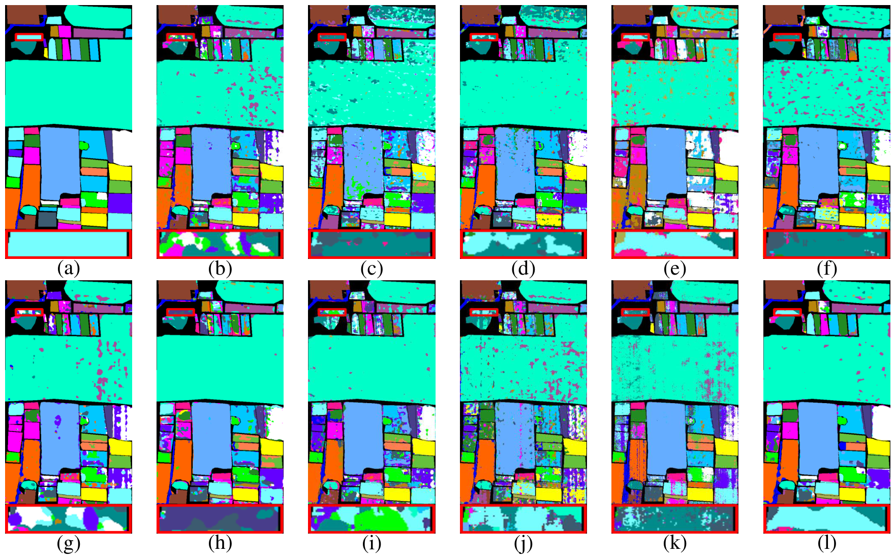
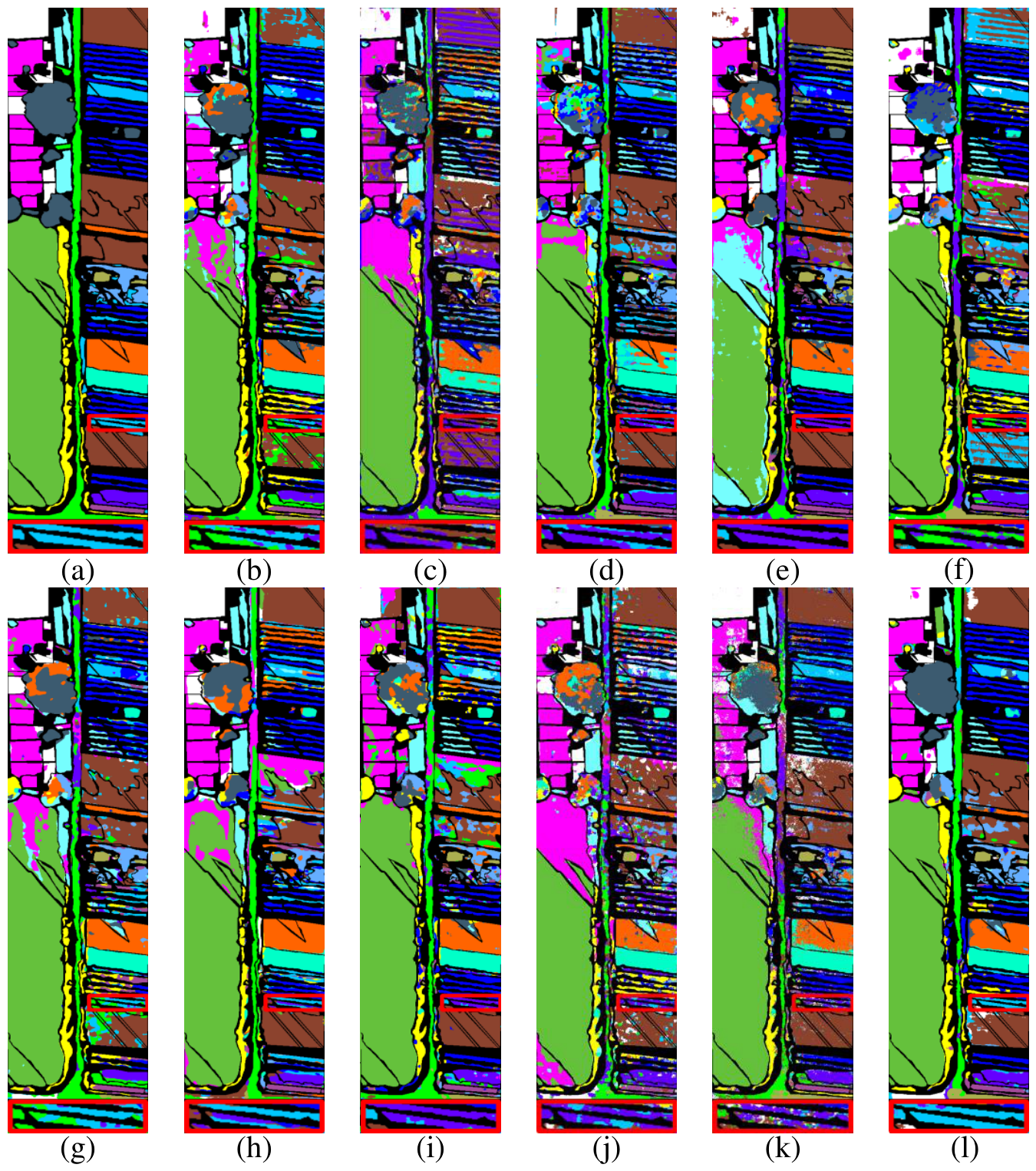
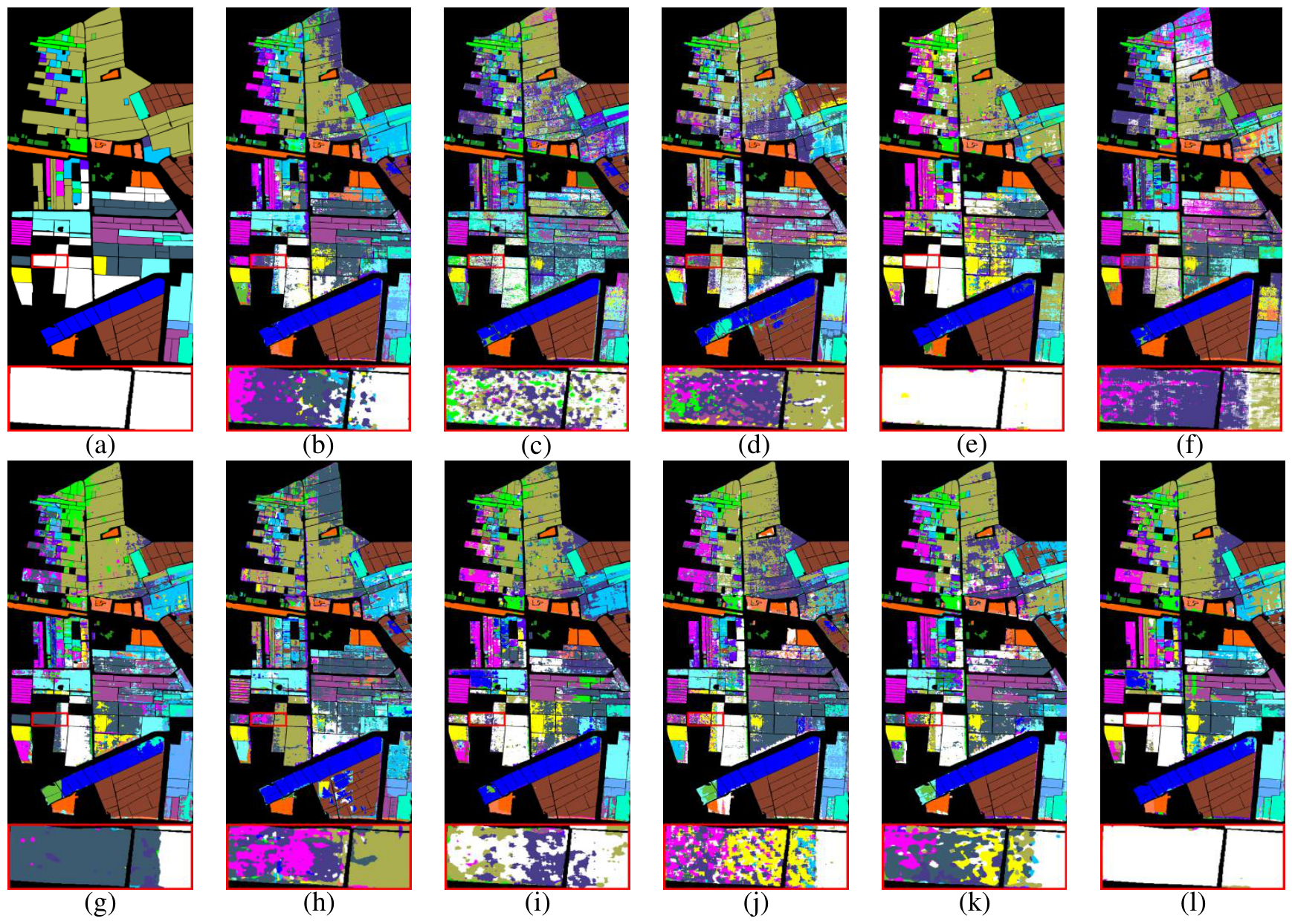
To evaluate the effectiveness of the proposed method, we present the qualitative classification maps for the HongHu, HanChuan, and XiongAn datasets in Figure 8, Figure 9 and Figure 10. By comparing our approach with the ten SOTA methods, the limitations of the baseline models in handling five-training-sample conditions become evident.

In contrast, our method achieves visual classification maps that most closely resemble the ground truth, characterized by significantly reduced isolated noise, globally coherent regions, and sharply delineated boundaries. At the spatial level, the asymmetric architecture adopts differentiated processing across resolutions to capture robust multi-scale features. Concurrently, the DMB’s Gaussian prior suppresses local interference by accurately focusing on central targets. At the spectral level, the PCA spectral decay prior explicitly directs the network to emphasize informative principal bands, thereby filtering out redundant spectral noise under limited samples. At the feature-space level, the SupCon regularization imposes explicit manifold constraints. By utilizing implicit hard sample mining to enforce strict intra-class compactness and inter-class dispersion, it effectively compensates for the limitations of the standard CE loss. Together, these three dimensions yield the exceptionally smooth and accurate visual results observed.

4.5. Ablation Study

To validate our core contributions, we conduct an ablation study isolating the impacts of the asymmetric multi-scale architecture, DMB, and SupCon regularization. The quantitative results across three benchmark datasets are reported in

Table 6. Ablation results under 5-shot setting. Disabling ‘multi-scale’, ‘DMB’, and ‘SupCon’ indicates reverting to a single-scale branch, retaining the dual-branch without priors, and optimizing solely with CE loss, respectively. × denotes removing the corresponding component, while ✓ denotes adding it.

Multi-Scale	DMB	SupCon	HanChuan			HongHu			XiongAn
			OA	AA	Kappa	OA	AA	Kappa	OA	AA	Kappa
×	×	×	$79.60\pm 3.42$	$78.24\pm 1.71$	$76.44\pm 3.80$	$86.49\pm 1.28$	$82.51\pm 1.37$	$83.08\pm 1.56$	$65.50\pm 2.23$	$73.51\pm 0.83$	$61.76\pm 2.25$
×	✓	✓	$81.56\pm 3.27$	$81.03\pm 1.87$	$78.70\pm 3.66$	$87.75\pm 1.10$	$84.80\pm 1.52$	$84.65\pm 1.33$	$65.90\pm 2.55$	$75.28\pm 1.16$	$62.27\pm 2.63$
×	×	✓	$81.69\pm 2.99$	$81.46\pm 1.97$	$78.86\pm 3.34$	$87.45\pm 1.36$	$84.90\pm 1.33$	$84.31\pm 1.61$	$65.50\pm 2.60$	$74.99\pm 1.26$	$62.12\pm 2.87$
×	✓	×	$80.79\pm 2.75$	$80.44\pm 1.41$	$77.82\pm 3.06$	$87.29\pm 1.18$	$84.04\pm 1.76$	$84.07\pm 1.46$	$64.92\pm 2.55$	$73.74\pm 1.20$	$61.16\pm 2.67$
✓	×	✓	$82.38\pm 2.65$	$81.25\pm 1.51$	$79.64\pm 2.92$	$87.99\pm 1.19$	$85.04\pm 1.68$	$84.93\pm 1.47$	$66.98\pm 2.12$	$75.94\pm 0.94$	$63.37\pm 2.17$
✓	×	×	$82.50\pm 2.84$	$81.32\pm 2.07$	$79.75\pm 3.24$	$87.93\pm 1.29$	$84.66\pm 1.48$	$84.86\pm 1.73$	$66.43\pm 2.01$	$75.28\pm 1.03$	$63.08\pm 2.23$
✓	✓	×	$82.19\pm 3.09$	$81.52\pm 2.27$	$79.40\pm 3.48$	$88.01\pm 1.12$	$85.31\pm 1.33$	$84.96\pm 1.37$	$67.27\pm 2.00$	$76.16\pm 0.92$	$63.66\pm 2.09$
✓	✓	✓	$82.90\pm 2.48$	$81.42\pm 1.81$	$80.18\pm 2.79$	$88.25\pm 0.94$	$85.46\pm 1.34$	$85.25\pm 1.17$	$67.35\pm 1.96$	$76.08\pm 0.90$	$63.73\pm 2.06$

.

Removing multi-scale design causes a consistent decline in all metrics across all datasets, such as the OA on HanChuan dropping to 81.56%. This occurs because a single-scale branch fails to adaptively capture features of varying crop sizes and results in the loss of the asymmetric architecture, making it impossible to apply differentiated and fine-grained processing across different resolutions.

Removing the dual physical prior guidance from the DMB causes a performance bottleneck, with the OA on the HongHu dataset stagnating at 87.99%. This stems from the model losing explicit focal cues under extreme five-training-samples conditions. Without the constraints of Gaussian spatial and PCA spectral decay priors, the network cannot precisely focus on the central target and informative bands, making it highly vulnerable to high-dimensional background noise and spectral redundancy.

To further verify the effectiveness of each core component in DMB, we decoupled the independent contributions of its two internal priors. The experimental results are presented in

Table 7. Ablation study on spatial and spectral priors under the 5-shot setting. ‘Spatial prior’ and ‘spectral prior’ denote the adaptive Gaussian mask and the PCA-inspired spectral decay prior, respectively. × denotes removing the corresponding component, while ✓ denotes adding it.

Spatial Prior	Spectral Prior	HanChuan			HongHu			XiongAn
		OA	AA	Kappa	OA	AA	Kappa	OA	AA	Kappa
✓	×	82.45 ± 3.28	81.33 ± 1.81	79.71 ± 3.64	88.20 ± 1.21	85.41 ± 1.40	85.21 ± 1.49	67.08 ± 2.21	76.03 ± 1.08	63.62 ± 2.30
×	✓	82.56 ± 2.27	81.27 ± 1.78	80.11 ± 2.54	87.95 ± 1.62	85.23 ± 1.49	84.93 ± 1.93	67.16 ± 1.82	76.05 ± 0.84	63.57 ± 1.84
✓	✓	$82.90\pm 2.48$	$81.42\pm 1.81$	$80.18\pm 2.79$	$88.25\pm 0.94$	$85.46\pm 1.34$	$85.25\pm 1.17$	$67.35\pm 1.96$	$76.08\pm 0.90$	$63.73\pm 2.06$

. It is evident that removing either the spatial prior or the spectral prior in isolation consistently leads to performance degradation, although the extent of the drop varies across datasets. Take the HanChuan dataset as an example. Removing the spatial prior reduced the OA from 82.90% to 82.45%, while removing the spectral prior led to a drop to 82.56%. These results indicate that both priors play a statistically meaningful auxiliary role. The spatial prior tends to emphasize feature responses in central regions, thereby imposing weaker constraints on the periphery. The spectral prior, by contrast, provides a smooth decay bias along the channel dimension. This encourages the network to preferentially exploit principal component features with richer information. The best performance is achieved when both priors are combined, suggesting that their contributions are complementary.

To gain a fuller picture of the Gaussian spatial prior, we further inspected the per-class accuracy. Take the HanChuan dataset as an example. For blocky land-cover types such as strawberry, introducing the spatial prior raised the accuracy from 81.55% to 84.35%—an improvement of 2.80 percentage points. In contrast, for linear features such as roads, accuracy slightly declined after incorporating the prior, dropping from 74.32% to 70.35%. This phenomenon can be traced to the design of the Gaussian mask. The mask is designed to enhance the response at the central pixel, which naturally suits compact, blocky land-cover types like strawberry. For linear features such as roads, however, useful information extends along a specific direction rather than concentrating in the central neighborhood. The center-enhancing inductive bias therefore offers limited benefit in these cases; it may even slightly suppress contextual information along road edges, producing a mild negative effect. The experimental results suggest that despite a slight accuracy drop for the road class, the overall OA improves substantially. This indicates that the global gain provided by the spatial prior can, to a large extent, compensate for its local negative impact on individual classes.

Removing the SupCon regularization leads to a noticeable decline in OA and Kappa across all datasets. While AA exhibits marginal fluctuations of around 0.1 percent well within statistical variance, the overall degradation indicates that relying solely on standard cross-entropy loss often causes feature-space collapse under limited samples. SupCon prevents this severe overfitting by imposing explicit manifold constraints to firmly separate confusing samples, thereby securing superior global classification consistency.

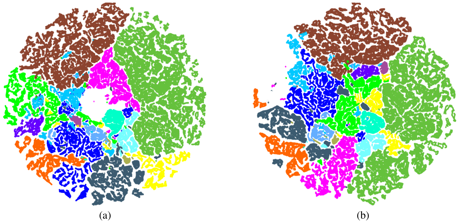
To more intuitively illustrate how supervised contrastive (SupCon) regularization refines the feature distribution, we have added a t-stochastic neighbor embedding (t-SNE) visualization of the feature space in Figure 11. As shown in Figure 11b, when relying solely on the standard cross-entropy loss, the sample distribution in the feature space is relatively loose. Some inter-class boundaries remain insufficiently clear, accompanied by a certain degree of feature overlap and confusion. This indicates that the single CE loss, lacking explicit manifold constraints, presents certain limitations in distinguishing complex crop classes with highly similar spectral characteristics.

In contrast, as shown in Figure 11a, the structure of the feature distribution is improved to a certain extent after introducing SupCon regularization. Benefiting from its implicit hard sample mining mechanism, features of the same class show a better clustering tendency, with relatively more compact clusters. Meanwhile, the separation between feature clusters of different classes is enhanced, reducing confusion in the boundary regions. This further indicates that SupCon regularization helps optimize the manifold structure of the feature space. It provides beneficial constraints to alleviate feature collapse under extremely limited sample conditions.

Ultimately, the absence of any core component restricts the model’s representative capacity. Only through the concurrent integration of the multi-scale architecture, dual prior guidance, and SupCon regularization, DPMSCH-Net can achieve peak metrics across all datasets, demonstrating superior classification performance and exceptional robustness under extreme five-training-samples conditions.

5. Conclusions

This paper proposed DPMSCH-Net model, a dual prior-guided multi-scale asymmetric architecture tailored for FSL-HSIC. By integrating an asymmetric SSM-CNN framework, DMB, and SupCon regularization, the model achieves superior feature representation under extreme label scarcity. Specifically, the asymmetric multi-scale SSM-CNN architecture performs feature extraction through three parallel branches with decreasing resolutions. While utilizing Mamba to process high-resolution features and selectively introducing HCM into higher-resolution branches for fine-grained aggregation, it employs lightweight convolutions to process heavily downsampled information, thereby efficiently capturing multi-scale spatial features. The DMB leverages adaptive Gaussian spatial and spectral guidance priors to guide the model to selectively prioritize the central target region and the most informative spectral bands, while avoiding excessive suppression of peripheral spatial features or low-energy spectral channels. Meanwhile, the SupCon regularization mechanism explicitly constrains the feature topology via implicit hard sample mining, effectively preventing feature collapse and enhancing intra-class compactness and inter-class dispersion without the need for tedious sample pair construction.

While DPMSCH-Net provides a highly effective solution for label-scarce scenarios, its current evaluation is limited to agricultural UAV scenes with similar spectral ranges from 400 to 1000 nm. Its generalizability to other HSI domains, such as urban remote sensing, geological mapping, or satellite-borne sensors, remains unexplored. Future work will focus on investigating this cross-domain adaptability and further lightweight the model for large-scale monitoring applications.

References

1. Wu, C.; Feng, R.; Zhang, P.; Mao, H.; Wang, D.; Bai, Z.; Li, Y. MRC-Net: A Multistage Network with Rank-Reduced Multihead Self-Attention and Cascade Learning for Hyperspectral Pansharpening. IEEE J. Sel. Top. Appl. Earth Obs. Remote Sens. 2025, 18, 22466–22485. [Google Scholar] [CrossRef]
2. Lebedev, L.I.; Yasakov, Y.V.; Utesheva, T.H.; Gromov, V.P.; Borusjak, A.V.; Turlapov, V. Complex analysis and monitoring of the environment based on Earth sensing data. Comput. Opt. 2019, 43, 282–295. [Google Scholar] [CrossRef]
3. Chen, X.; Zheng, X.; Zhang, Y.; Lu, X. Remote sensing scene classification by local–global mutual learning. IEEE Geosci. Remote Sens. Lett. 2022, 19, 6506405. [Google Scholar] [CrossRef]
4. Pasolli, E.; Melgani, F.; Tuia, D.; Pacifici, F.; Emery, W.J. SVM Active Learning Approach for Image Classification Using Spatial Information. IEEE Trans. Geosci. Remote Sens. 2014, 52, 2217–2233. [Google Scholar] [CrossRef]
5. Ma, L.; Crawford, M.M.; Tian, J. Local Manifold Learning-Based k-Nearest-Neighbor for Hyperspectral Image Classification. IEEE Trans. Geosci. Remote Sens. 2010, 48, 4099–4109. [Google Scholar]
6. Ham, J.; Chen, Y.; Crawford, M.M.; Ghosh, J. Investigation of the random forest framework for classification of hyperspectral data. IEEE Trans. Geosci. Remote Sens. 2005, 43, 492–501. [Google Scholar] [CrossRef]
7. Wu, C.; Wang, D.; Bai, Y.; Mao, H.; Li, Y.; Shen, Q. HSR-Diff: Hyperspectral image super-resolution via conditional diffusion models. In Proceedings of the IEEE/CVF International Conference on Computer Vision (ICCV); IEEE: Piscataway, NJ, USA, 2023; pp. 7060–7070. [Google Scholar]
8. Zhong, Z.; Li, J.; Luo, Z.; Chapman, M. Spectral–spatial residual network for hyperspectral image classification: A 3-D deep learning framework. IEEE Trans. Geosci. Remote Sens. 2018, 56, 847–858. [Google Scholar] [CrossRef]
9. Song, W.; Li, S.; Fang, L.; Lu, T. Hyperspectral image classification with deep feature fusion network. IEEE Trans. Geosci. Remote Sens. 2018, 56, 3173–3184. [Google Scholar] [CrossRef]
10. Zhao, Z.; Xu, X.; Li, S.; Plaza, A. Hyperspectral Image Classification Using Groupwise Separable Convolutional Vision Transformer Network. IEEE Trans. Geosci. Remote Sens. 2024, 62, 5511817. [Google Scholar] [CrossRef]
11. Hong, D.; Han, Z.; Yao, J.; Gao, L.; Zhang, B.; Plaza, A.; Chanussot, J. SpectralFormer: Rethinking Hyperspectral Image Classification with Transformers. IEEE Trans. Geosci. Remote Sens. 2022, 60, 5518615. [Google Scholar] [CrossRef]
12. Zhang, J.; Liu, L.; Zhao, R.; Shi, Z. A Bayesian meta-learning-based method for few-shot hyperspectral image classification. IEEE Trans. Geosci. Remote Sens. 2023, 61, 5500613. [Google Scholar] [CrossRef]
13. Li, W.; Liu, Q.; Zhang, Y.; Wang, Y.; Yuan, Y.; Jia, Y.; He, Y. Few-shot hyperspectral image classification using meta learning and regularized finetuning. IEEE Trans. Geosci. Remote Sens. 2023, 61, 5529514. [Google Scholar] [CrossRef]
14. Wang, W.; Liu, F.; Xiao, L. I2MEP-Net: Inter- and intra-modality enhancing prototypical network for few-shot hyperspectral image classification. IEEE Trans. Geosci. Remote Sens. 2024, 62, 5516815. [Google Scholar] [CrossRef]
15. Gao, K.; Liu, B.; Yu, X.; Qin, J.; Zhang, P.; Tan, X. Deep relation network for hyperspectral image few-shot classification. Remote Sens. 2020, 12, 923. [Google Scholar] [CrossRef]
16. Zeng, J.; Xue, Z.; Zhang, L.; Lan, Q.; Zhang, M. Multistage relation network with dual-metric for few-shot hyperspectral image classification. IEEE Trans. Geosci. Remote Sens. 2023, 61, 5510017. [Google Scholar] [CrossRef]
17. Deng, B.; Jia, S.; Shi, D. Deep metric learning-based feature embedding for hyperspectral image classification. IEEE Trans. Geosci. Remote Sens. 2020, 58, 1422–1435. [Google Scholar] [CrossRef]
18. Zhu, L.; Chen, Y.; Ghamisi, P.; Benediktsson, J.A. Generative adversarial networks for hyperspectral image classification. IEEE Trans. Geosci. Remote Sens. 2018, 56, 5046–5063. [Google Scholar] [CrossRef]
19. Li, W.; Wu, G.; Zhang, F.; Du, Q. Hyperspectral image classification using deep pixel-pair features. IEEE Trans. Geosci. Remote Sens. 2017, 55, 844–853. [Google Scholar] [CrossRef]
20. Nalepa, J.; Myller, M.; Kawulok, M. Training- and test-time data augmentation for hyperspectral image segmentation. IEEE Geosci. Remote Sens. Lett. 2020, 17, 292–296. [Google Scholar] [CrossRef]
21. Zhang, H.; Cisse, M.; Dauphin, Y.N.; Lopez-Paz, D. mixup: Beyond empirical risk minimization. In Proceedings of the 6th International Conference on Learning Representations (ICLR); OpenReview.net: Vancouver, BC, Canada, 2018. [Google Scholar]
22. Wang, D.; Bai, Y.; Wu, C.; Li, Y.; Shang, C.; Shen, Q. Convolutional LSTM-based hierarchical feature fusion for multispectral pan-sharpening. IEEE Trans. Geosci. Remote Sens. 2022, 60, 5404016. [Google Scholar] [CrossRef]
23. Khosla, P.; Teterwak, P.; Wang, C.; Sarna, A.; Tian, Y.; Isola, P.; Maschinot, A.; Liu, C.; Krishnan, D. Supervised contrastive learning. Adv. Neural Inf. Process. Syst. 2020, 33, 18661–18673. [Google Scholar]
24. Chen, Y.; Lin, Z.; Zhao, X.; Wang, G.; Gu, Y. Deep learning-based classification of hyperspectral data. IEEE J. Sel. Top. Appl. Earth Obs. Remote Sens. 2014, 7, 2094–2107. [Google Scholar] [CrossRef]
25. Zhao, W.; Du, S. Spectral–spatial feature extraction for hyperspectral image classification: A dimension reduction and deep learning approach. IEEE Trans. Geosci. Remote Sens. 2016, 54, 4544–4554. [Google Scholar] [CrossRef]
26. Hu, W.; Huang, Y.; Wei, L.; Zhang, F.; Li, H. Deep convolutional neural networks for hyperspectral image classification. J. Sens. 2015, 2015, 258619. [Google Scholar] [CrossRef]
27. Li, Y.; Zhang, H.; Shen, Q. Spectral–spatial classification of hyperspectral imagery with 3D convolutional neural network. Remote Sens. 2017, 9, 67. [Google Scholar] [CrossRef]
28. Roy, S.K.; Krishna, G.; Dubey, S.R.; Chaudhuri, B.B. HybridSN: Exploring 3-D–2-D CNN feature hierarchy for hyperspectral image classification. IEEE Geosci. Remote Sens. Lett. 2020, 17, 277–281. [Google Scholar] [CrossRef]
29. Gong, Z.; Zhong, P.; Yu, Y.; Hu, W.; Li, S. A CNN with multiscale convolution and diversified metric for hyperspectral image classification. IEEE Trans. Geosci. Remote Sens. 2019, 57, 3599–3618. [Google Scholar] [CrossRef]
30. Paoletti, M.E.; Haut, J.M.; Fernandez-Beltran, R.; Plaza, J.; Plaza, A.J.; Pla, F. Deep pyramidal residual networks for spectral–spatial hyperspectral image classification. IEEE Trans. Geosci. Remote Sens. 2019, 57, 740–754. [Google Scholar] [CrossRef]
31. He, M.; Li, B.; Chen, H. Multi-scale 3D deep convolutional neural network for hyperspectral image classification. In 2017 IEEE International Conference on Image Processing (ICIP); IEEE: Piscataway, NJ, USA, 2017; pp. 3904–3908. [Google Scholar]
32. Xu, F.; Mei, S.; Zhang, G.; Wang, N.; Du, Q. Bridging CNN and transformer with cross-attention fusion network for hyperspectral image classification. IEEE Trans. Geosci. Remote Sens. 2024, 62, 5522214. [Google Scholar] [CrossRef]
33. Gu, A.; Dao, T. Mamba: Linear-time sequence modeling with selective state spaces. arXiv 2024, arXiv:2312.00752. [Google Scholar]
34. Zhu, L.; Liao, B.; Zhang, Q.; Wang, X.; Liu, W.; Wang, X. Vision Mamba: Efficient visual representation learning with bidirectional state space model. arXiv 2024, arXiv:2401.09417. [Google Scholar]
35. Liu, Y.; Tian, Y.; Zhao, Y.; Yu, H.; Xie, L.; Wang, Y.; Ye, Q.; Jiao, J.; Liu, Y. VMamba: Visual state space model. Adv. Neural Inf. Process. Syst. 2024, 37, 103031–103063. [Google Scholar] [CrossRef]
36. Li, Y.; Luo, Y.; Zhang, L.; Wang, Z.; Du, B. MambaHSI: Spatial–spectral Mamba for hyperspectral image classification. IEEE Trans. Geosci. Remote Sens. 2024, 62, 5524216. [Google Scholar] [CrossRef]
37. Wang, Y.; Liu, L.; Xiao, J.; Yu, D.; Tao, Y.; Zhang, W. MambaHSI+: Multidirectional state propagation for efficient hyperspectral image classification. IEEE Trans. Geosci. Remote Sens. 2025, 63, 4411414. [Google Scholar] [CrossRef]
38. Mao, J.; Ma, H.; Liang, Y. BiMambaHSI: Bidirectional spectral–spatial state space model for hyperspectral image classification. Remote Sens. 2025, 17, 3676. [Google Scholar] [CrossRef]
39. He, Y.; Tu, B.; Liu, B.; Li, J.; Plaza, A. 3DSS-Mamba: 3D-spectral-spatial Mamba for hyperspectral image classification. IEEE Trans. Geosci. Remote Sens. 2024, 62, 5534216. [Google Scholar] [CrossRef]
40. Xu, Y.; Han, C.; Chen, S.; Jin, Y.; Miao, Y.; Guo, H.; Wang, D. PHDMamba: Progressive hybrid Mamba for hyperspectral image classification. IEEE Geosci. Remote Sens. Lett. 2025, 22, 5510605. [Google Scholar] [CrossRef]
41. Yang, X.; Wei, Y.; Tan, J.; Li, S.; Tang, H.; Liu, W. LMamba: Local-guided Mamba with multi-scale filtering for hyperspectral image classification. Remote Sens. 2026, 18, 1629. [Google Scholar] [CrossRef]
42. Fang, Y.; Sun, L.; Zheng, Y.; Wu, Z. Deformable convolution-enhanced hierarchical transformer with spectral–spatial cluster attention for hyperspectral image classification. IEEE Trans. Image Process. 2025, 34, 701–716. [Google Scholar] [CrossRef]
43. Xi, B.; Zhang, Y.; Li, J.; Zheng, T.; Zhao, X.; Xu, H.; Xue, C.; Li, Y.; Chanussot, J. MCTGCL: Mixed CNN–Transformer for Mars hyperspectral image classification with graph contrastive learning. IEEE Trans. Geosci. Remote Sens. 2025, 63, 5503214. [Google Scholar] [CrossRef]
44. Zhang, J.; Li, L.; Jiao, L.; Liu, X.; Liu, F.; Ma, W.; Yang, S.; Chen, P. PIMamba: Physics-Informed Mamba for Few-Shot Hyperspectral Image Classification. IEEE Trans. Geosci. Remote Sens. 2026, 64, 5511116. [Google Scholar] [CrossRef]
45. Li, J.; Wu, H.; Song, R.; Xu, H.; Li, Y.; Du, Q. Physics-Guided Time-Interactive-Frequency Network for Cross-Domain Few-Shot Hyperspectral Image Classification. IEEE Trans. Neural Netw. Learn. Syst. 2026, 37, 438–452. [Google Scholar] [CrossRef] [PubMed]
46. He, Y.; Tu, B.; Liu, B.; Li, J.; Plaza, A. HSI-MFormer: Integrating Mamba and Transformer experts for hyperspectral image classification. IEEE Trans. Geosci. Remote Sens. 2025, 63, 5621916. [Google Scholar] [CrossRef]
47. Sheng, J.; Zhou, J.; Wang, J.; Ye, P.; Fan, J. DualMamba: A Lightweight Spectral–Spatial Mamba-Convolution Network for Hyperspectral Image Classification. IEEE Trans. Geosci. Remote Sens. 2025, 63, 5501415. [Google Scholar] [CrossRef]
48. Hou, S.; Shi, H.; Cao, X.; Zhang, X.; Jiao, L. Hyperspectral Imagery Classification Based on Contrastive Learning. IEEE Trans. Geosci. Remote Sens. 2022, 60, 5521213. [Google Scholar] [CrossRef]
49. Lee, H.; Kwon, H. Self-Supervised Contrastive Learning for Cross-Domain Hyperspectral Image Representation. In ICASSP 2022—2022 IEEE International Conference on Acoustics, Speech and Signal Processing; IEEE: Piscataway, NJ, USA, 2022; pp. 3239–3243. [Google Scholar]
50. Ayuba, D.L.A.; Guillemaut, J.Y.; Marti-Cardona, B.; Mendez, O. HyperKon: A Self-Supervised Contrastive Network for Hyperspectral Image Analysis. Remote Sens. 2024, 16, 3399. [Google Scholar] [CrossRef]
51. Huang, L.; Chen, Y.; He, X.; Ghamisi, P. Supervised Contrastive Learning-Based Classification for Hyperspectral Image. Remote Sens. 2022, 14, 5530. [Google Scholar] [CrossRef]
52. Schroff, F.; Kalenichenko, D.; Philbin, J. FaceNet: A unified embedding for face recognition and clustering. In Proceedings of the IEEE Conference on Computer Vision and Pattern Recognition (CVPR); IEEE: Piscataway, NJ, USA, 2015; pp. 815–823. [Google Scholar]
53. Wen, Y.; Zhang, K.; Li, Z.; Qiao, Y. A discriminative feature learning approach for deep face recognition. In Computer Vision—ECCV 2016; Springer International Publishing: Cham, Switzerland, 2016; pp. 499–515. [Google Scholar]
54. Li, S.; Song, W.; Fang, L.; Chen, Y.; Ghamisi, P.; Benediktsson, J.A. Deep Learning for Hyperspectral Image Classification: An Overview. IEEE Trans. Geosci. Remote Sens. 2019, 57, 6690–6709. [Google Scholar] [CrossRef]
55. Zhang, B.; Chen, Y.; Xiong, S.; Lu, X. Hyperspectral image classification via cascaded spatial cross-attention network. IEEE Trans. Image Process. 2025, 34, 899–913. [Google Scholar] [CrossRef]
56. Liu, S.; Fu, C.; Duan, Y.; Wang, X.; Luo, F. Spatial–spectral enhancement and fusion network for hyperspectral image classification with few labeled samples. IEEE Trans. Geosci. Remote Sens. 2025, 63, 5502414. [Google Scholar] [CrossRef]
57. Xu, Y.; Wang, D.; Zhang, L.; Zhang, L. Dual selective fusion transformer network for hyperspectral image classification. Neural Netw. 2025, 187, 107311. [Google Scholar] [CrossRef] [PubMed]
58. He, Y.; Tu, B.; Jiang, P.; Liu, B.; Li, J.; Plaza, A. IGroupSS-Mamba: Interval group spatial–spectral Mamba for hyperspectral image classification. IEEE Trans. Geosci. Remote Sens. 2024, 62, 5538817. [Google Scholar] [CrossRef]
Figure 1. Overall architecture of proposed method. The model jointly models spatial–spectral features via (dual Mamba block) DMB, performs hierarchical extraction along three branches of decreasing resolutions, and introduces a hierarchical context module (HCM) in the first two branches for fine-grained context aggregation, enabling accurate classification.
Remotesensing 18 02452 g001
Figure 2. Detailed architecture of DMB. (a) The SpaMamba submodule models spatial contexts guided by an adaptive Gaussian prior to emphasize central region features. (b) The SpeMamba submodule captures spectral dependencies by a spectral decay prior to focus on the informative principal channels.
Remotesensing 18 02452 g002
Figure 3. False-color images and GT for three datasets used in experiments. Different colors in the GT maps represent different land-cover classes, consistent with the color legend in Table 1. (a) HongHu, (b) HanChuan, and (c) XiongAn.
Remotesensing 18 02452 g003
Figure 4. Performance of the model with different retained dimensions of PCA c. (a) HongHu dataset, (b) HanChuan dataset, and (c) XiongAn dataset.
Remotesensing 18 02452 g004
Figure 5. Performance of the model with different input patch sizes w. (a) HongHu dataset, (b) HanChuan dataset, and (c) XiongAn dataset.
Remotesensing 18 02452 g005
Figure 6. Performance of the model with different parameters for the PCA spectral prior ϵ spe . (a) HongHu dataset, (b) HanChuan dataset, and (c) XiongAn dataset.
Remotesensing 18 02452 g006
Figure 7. Performance of the model with different parameters for the Gaussian spatial prior ϵ spa . (a) HongHu dataset, (b) HanChuan dataset, and (c) XiongAn dataset.
Remotesensing 18 02452 g007
Figure 8. Qualitative visualization of the classification map for the HongHu dataset. Different colors represent different land-cover classes (see the color legend for the HongHu dataset in Table 1), and red boxes highlight specific magnified regions for detailed comparison. (a) Ground truth, (b) IGroupSS-Mamba, (c) GSC-VIT, (d) MambaHSI, (e) SCluster-Former, (f) DSFormer, (g) HSI-MFormer, (h) MambaHSI+, (i) MCTGCL, (j) CSCANet, (k) SSEFN, and (l) DPMSCH-Net.
Remotesensing 18 02452 g008
Figure 9. Qualitative visualization of the classification map for the HanChuan dataset. Different colors represent different land-cover classes (see the color legend for the HanChuan dataset in Table 1), and red boxes highlight specific magnified regions for detailed comparison. (a) Ground truth, (b) IGroupSS-Mamba, (c) GSC-VIT, (d) MambaHSI, (e) SCluster-Former, (f) DSFormer, (g) HSI-MFormer, (h) MambaHSI+, (i) MCTGCL, (j) CSCANet, (k) SSEFN, and (l) DPMSCH-Net.
Remotesensing 18 02452 g009
Figure 10. Qualitative visualization of the classification map for XiongAn dataset. Different colors represent different land-cover classes (see the color legend for the XiongAn dataset in Table 1), and red boxes highlight specific magnified regions for detailed comparison. (a) Ground truth, (b) IGroupSS-Mamba, (c) GSC-VIT, (d) MambaHSI, (e) SCluster-Former, (f) DSFormer, (g) HSI-MFormer, (h) MambaHSI+, (i) MCTGCL, (j) CSCANet, (k) SSEFN, and (l) DPMSCH-Net.
Remotesensing 18 02452 g010
Figure 11. Demonstration of the impact of the SupCon regularization on the HanChuan dataset. (a) T-SNE visualization with SupCon regularization; (b) T-SNE visualization without SupCon regularization. The color-to-class mapping is provided in Table 1 HanChuan dataset.
Remotesensing 18 02452 g011