


Highlights
What are the main findings?
- This paper proposes an ESGS algorithm that can effectively reconstruct 3D Martian scenes from optical remote sensing image sequences of the Martian surface.
- This paper constructs a COLMAP-format Martian 3D reconstruction dataset called Mars_3D.
What are the implications of the main findings?
- The proposed algorithm can provide insights into improving the accuracy of 3D reconstruction of the Martian surface.
- The constructed Martian 3D dataset in the standard COLMAP format can serve as training material for research related to Martian 3D reconstruction, terrain mapping, and landform analysis.
Abstract
Mars exploration is an advanced field of global deep space exploration. Accurate three-dimensional reconstruction of the Martian surface topography is very important for autonomous navigation, scientific target recognition, and operation planning. In order to meet the analysis requirements of the Martian surface scene, this paper proposes an explicit surface-geometry-constrained Gaussian splatting (ESGS) method. Firstly, this method includes a normal and depth prior estimation network (NDN) that generates normal and depth priors from Martian surface image data, thereby promoting the fusion of semantic and multi-view contextual information to enhance the geometric accuracy of 3D reconstruction of the Martian surface. Secondly, we designed the Gaussian parameter-based deformable fusion network (GPDFN) to fuse multi-receptive-field feature information. Finally, we collected Martian surface remote sensing images from NASA, constructed a Martian surface 3D reconstruction dataset named Mars_3D using the COLMAP method, annotated depth and normal labels for its seven real-world scenes and two Blender-generated scenes, and conducted comparative experiments with eight excellent algorithms on this dataset to validate the effectiveness of our method in 3D reconstruction of the Martian surface using remote sensing images. Experiments show that the average SSIM of the ESGS method in this article is 0.6946, PSNR is 23.40 dB, and LPIPS is 0.253 on the Mars_3D dataset, demonstrating superior overall performance compared to all other models and enhancing the quality of 3D reconstruction of the Martian surface.
1. Introduction
In Mars exploration missions, on the one hand, the Mars rover needs to move and operate within a fixed area. However, numerous rocks, craters, steep slopes, and sandy terrain on the Martian surface [1,2,3] limit the rover’s progress. It significantly reduces its surface exploration efficiency, potentially even severely impairing its functionality. Therefore, it is critical to avoid restricted areas, ensure that the rover can operate normally under dusty conditions with guidance from a 3D map, achieve 3D reconstruction of the Martian surface, and enable automatic multi-scenario operations. On the other hand, before a rover is launched to Mars to perform tasks such as exploration, patrol, and sampling, its camera imaging, mechanical structure control, and command transmission/reception functions must be tested on Earth to develop contingency solutions. In this context, the 3D reconstruction of the Martian surface can serve as a functional simulation test, i.e., a virtual scene for closed-loop simulation, providing more realistic Martian data for Earth-based testing.
Martian surface landforms not only record the geological evolution of the planet but also serve as direct work areas for rover landing, path planning, and robotic arm operations, thereby holding significant scientific and engineering value for ensuring the safety and efficient execution of exploration missions. However, due to the harsh Martian environment [4,5,6] and the prohibitively high cost of exploration, terrain data acquired by orbiters and rovers often suffer from occlusions, sparse viewpoints, or incompleteness, making it difficult to directly construct complete 3D models suitable for algorithm training and mission validation. To achieve the 3D reconstruction of the aforementioned Martian landforms, digitization represents a highly important and practical approach, offering advantages such as convenient storage, diverse presentation methods, and broad applicability across education, scientific research, and other cross-disciplinary fields. Common terrain digitization methods include LiDAR 3D scanning for generating point cloud data, 3D terrain generation from high-resolution images, and panoramic camera-based digital storage.
In the field of deep space reconstruction, Chen et al. proposed Mars3DNet [7] in 2021, a CNN-based twin-network framework trained on paired synthetic and real data that can recover topographic details of the Martian surface from a single Martian image. In 2025, Cao et al. proposed LoGAN [8], a local attention generative adversarial network that can achieve detailed 3D terrain reconstruction of the Martian surface from a single image. In 2026, Zou et al. proposed the PFMGAN [9] algorithm, which takes the solar angle as an explicit conditional input and incorporates an albedo-aware attention module. This method was tested on five types of Martian landforms, including volcanoes and impact craters, and its reconstruction accuracy significantly surpasses that of purely data-driven models. This study primarily uses visible-light remote sensing images captured by Mars rovers, adopts the 3D Gaussian splatting (3DGS) [10] image processing algorithm as the baseline model, and proposes the ESGS algorithm, which reconstructs the Martian surface in 3D using only the most readily accessible 2D images.
In recent years, the 3DGS method based on deep learning has demonstrated excellent performance in generating 3D scenes from image sequences, gradually becoming the mainstream algorithm in 3D reconstruction. In 2023, the 3DGS method first appeared in the public eye, using three-dimensional Gaussian functions to represent scenes, accelerating rendering speed, and improving scene optimization quality. Its use of SFM [11], spherical harmonics [12], volume rendering [13], and related formulas provides a feasible solution for subsequent research on 3D reconstruction. In 2024, in order to improve the geometric accuracy of 3D reconstruction, 2DGS [14] proposed the idea that rendering 3D scenes only requires surface reconstruction, using two regularization terms, depth consistency and normal consistency, to constrain Gaussian functions. In the same year, ScaffoldGS [15] used point cloud voxelization and voxel growth methods to address the problems of excessive Gaussian function redundancy and poor robustness to camera view changes. Mip-Splatting [16] proposed using low-pass and Mip filters to limit high-frequency signals and expand the imaging scale, thereby addressing problems such as noise aliasing and high-frequency glitches in rendered images.
In the field of dynamic scene 3D reconstruction, 3DGS also has many applications. In 2024, 4DGS [17] encodes image frame identifiers and Gaussian primitives into a unified feature vector and predicts the deformation of Gaussian functions using neural networks to gradually change the 3D scene over time t. In 2025, 4DGS-1K [18] proposed a compact, memory-efficient dynamic scene representation that significantly improved the storage and rasterization efficiency of 3D scenes, achieving 1000 FPS on a GPU. In addition, there are many 3D reconstruction algorithms, such as DeSiReGS [19], HUGS [20], PVG [21], StreetGS [22], F2Plenoxels [23], and DrivingGS [24], which offer many ideas for modeling dynamic scenes.
While the aforementioned algorithm achieves excellent 3D reconstruction results for indoor and outdoor scenes on Earth, it still encounters the following problems and challenges:
- Martian surface scenes exhibit large texture variations, containing both weak-texture and rich-texture regions. Some studies do not leverage explicit priors from depth and normal information to improve geometric accuracy, leading to noise and artifacts in low-texture regions.
- The Martian surface contains large continuous regions where the Gaussian parameters are correlated. Some studies fail to effectively fuse Gaussian features, thereby compromising the multi-view consistency of the Martian surface.
- Remote sensing images of the Martian surface are limited in number and captured from sparse viewpoints. Improving the accuracy and stability of 3D reconstruction of the Martian surface requires pre-training using Martian surface remote sensing images.
To address the above issues, we propose an ESGS 3D reconstruction algorithm for the Martian surface. The proposed method aims to enhance the geometric accuracy of 3D reconstruction and achieve the digitization of Martian landforms. To demonstrate the effectiveness of our algorithm, we conducted comprehensive experiments across multiple Martian scenes.
The main contributions of this paper are as follows:
- This paper proposed a three-dimensional reconstruction model for the Martian surface based on monocular optical remote sensing images called the ESGS to fuse Martian landform color, texture, and context information, promote the complementary learning of adjacent Gaussian ellipsoid parameters, and improve the accuracy of three-dimensional reconstruction of Martian landforms and the quality of image rendering.
- The ESGS algorithm uses 3DGS as the benchmark model, and we design and add an NDN network in the ESGS to address the lack of depth and normal information about objects in 3DGS, thereby improving the geometric accuracy of geomorphic reconstruction.
- We designed the GPDFN to fuse Gaussian feature information to enable complementary learning of Martian landform texture and other features and built a three-dimensional reconstruction dataset of Martian surface topography called Mars_3D, containing seven real scenes and two Blender virtual scenes. The dataset is rich in geomorphic details, including many Martian scenes with rocks, pits, steep slopes, and sand.
- We conducted a large number of comparative and ablation experiments across multiple datasets, comparing the proposed ESGS algorithm with eight advanced 3D reconstruction algorithms to verify the effectiveness of the research presented in this paper. Finally, the ESGS algorithm can achieve 3D reconstruction of the Martian surface and reduce noise artifacts generated during the reconstruction of some Martian landforms.
2. Related Works
Diffusion models have demonstrated powerful capabilities for image generation and inpainting. In the context of terrain inpainting, Lo and Peters proposed Diff-DEM [25], an algorithm based on DDPM [26] that addresses void-filling in digital elevation models. By progressively reconstructing missing terrain through a reverse diffusion process, it achieves superior inpainting results compared to GAN-based methods. Zhao et al. proposed a terrain-feature-guided diffusion model, TFDM [27], which introduces terrain gradients as prior information into the iterative process, effectively enhancing the geometric realism of digital terrain models. However, these methods are primarily developed for Earth data and rely heavily on conditional generation, making them difficult to directly apply to the Martian surface.
Catalano and Soccini addressed the inpainting of missing regions in Martian elevation maps [28] by training an unconditional DDPM model and employing a non-uniform resampling strategy to capture multi-scale terrain features, thereby achieving better visual consistency in 3D rendering of the inpainted Martian terrain. Nonetheless, research on directly applying diffusion models to 3D surface geometry reconstruction remains scarce, and their integration with 3DGS is still unexplored. Depth and normal estimation form the core foundation of monocular 3D reconstruction. In 2014, Eigen et al. proposed a single-image depth prediction algorithm based on a multi-scale CNN architecture [29], laying the groundwork for deep learning-based monocular depth estimation. For planetary surface geometry estimation, Hu et al. proposed a zero-shot geometric foundation model, Metric3D v2 [30], that jointly estimates depth and surface normals and exhibits excellent generalization performance on Martian images. Wang et al. proposed the VGGT algorithm [31], which robustly recovers intrinsic and extrinsic camera parameters, as well as depth maps, from sparse views, providing reliable geometric priors for 3D reconstruction. In the context of Mars rover localization, Kou et al. proposed the MarsCVFP framework [32], which combines multi-scale feature pyramids and designs a feature interaction module, effectively improving cross-view feature consistency in weak-texture regions.
Within the 3DGS framework, accurate depth and normal priors are crucial for updating Gaussian parameters and ensuring geometric consistency across the scene. Xu et al. proposed DepthSplat [33], which tightly couples depth estimation with Gaussian splatting and improves geometric reconstruction accuracy through depth regularization loss. Cong et al. proposed the VideoLifter framework [34] for monocular video 3D reconstruction, which employs hierarchical stereo alignment and segment fusion strategies to suppress error accumulation and effectively enhance multi-view geometric consistency. However, most existing depth estimation models are trained on Earth-based scenes, whose statistical distributions differ significantly from those of the Martian surface. In summary, current 3D reconstruction methods for the Martian surface still exhibit notable limitations in completeness of physical modeling, robustness to sparse viewpoints, and the ability to explicitly represent geometry. Based on this, this paper explores the use of the 3DGS algorithm, combined with explicit depth and normal constraints, to achieve high-precision 3D reconstruction of the Martian surface.
3. Materials and Methods
3.1. Dataset
3.1.1. Our Mars_3D Dataset
Currently, there is no publicly available COLMAP-format dataset for the 3D reconstruction of Martian landforms. Therefore, this paper creates the Mars_3D dataset to validate the effectiveness of the proposed improved model ESGS. The visible-light remote sensing images of the Martian surface used in this study are all sourced from the official NASA website and are free for non-commercial use. For details, please refer to https://www.nasa.gov/nasa-brand-center/images-and-media/ (accessed on 3 April 2026).
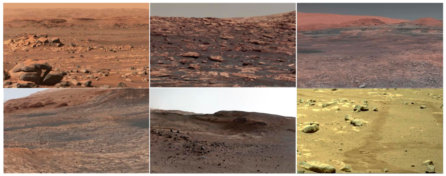
Some of the remote sensing images presented in the paper are not original images; instead, the original panoramas have been segmented into multiple images to facilitate subsequent 3D reconstruction. The segmented images have a resolution of 1920 × 1080, and the overlap rate between images ranges from 30% to 60%, selected based on the size of the panoramic image. To verify the robustness of the proposed algorithm, we also simulated Martian surface scenes using Blender and constructed virtual 3D Martian terrain. The dataset comprises 137 multi-view Martian landform images: 77 across 7 real scenes (average of 11 per scene) and 60 across 2 Blender virtual scenes (average of 30 per scene). The dataset encompasses diverse Martian landform features, including sandy ground, rocks, steep slopes, hills, and craters. It is rich in terrain characteristics, making it highly suitable for research on 3D reconstruction and digitization of the Martian surface. A subset of the remote sensing images from the Mars_3D dataset is shown in Figure 1.
Figure 1.
Some examples of the Mars_3D dataset.
To realize 3D reconstruction of Martian landforms, we also need to use feature correlation between image sequences, namely the overlapping area between images, to generate sparse point clouds for each landform scene and provide initial point clouds for subsequent algorithms. First, we need a set of Mars landform image sequences, as shown in Figure 2.
Figure 2.
Example of Mars landform image sequence.
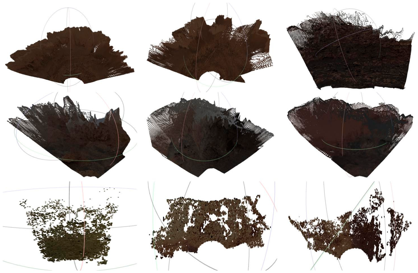
Then, we use the SFM method to construct a sparse point cloud of the landform, which does not need to be very accurate; it suffices to align with visual observations and image data. In the subsequent ESGS training process, the point cloud parameters will be updated by gradient backpropagation. Figure 3 shows the point cloud data for all nine scenes.
Figure 3.
Point cloud data of 9 scenarios.
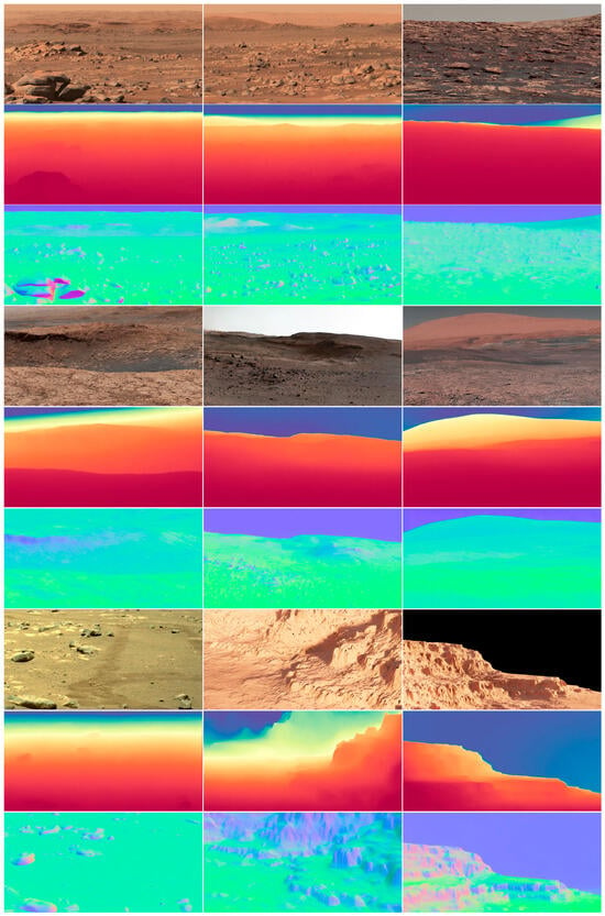
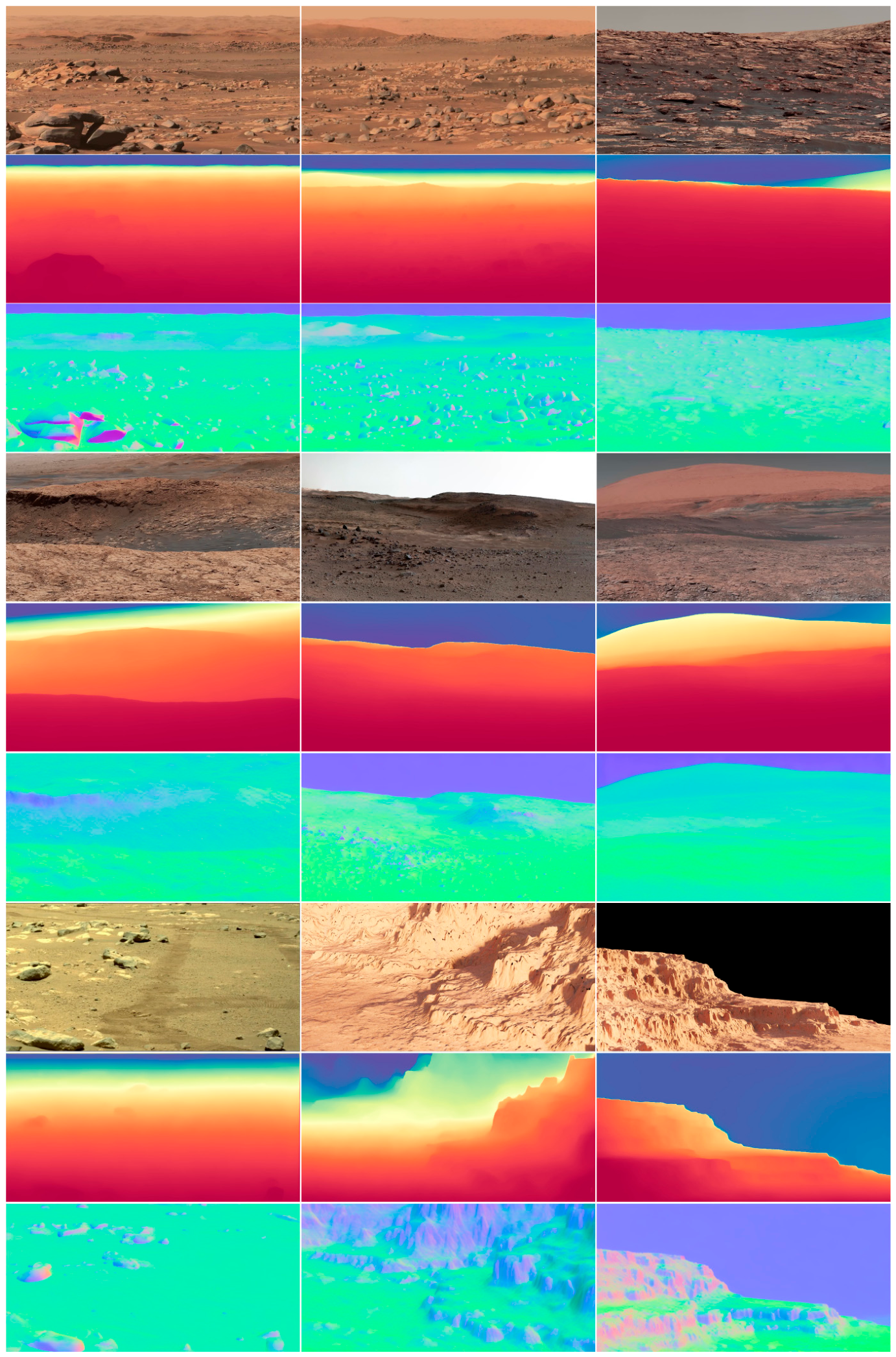
The original 3DGS algorithm is designed for real-time, high-fidelity novel-view synthesis. Each 3D Gaussian ellipsoid stores only position, color, opacity, and the covariance matrix, and the training process does not use depth or normal information from the 3D scene. As a result, the reconstructed 3D geometry exhibits an inaccurate geometric representation, and the derived depth and normal estimates are unreliable, leading to Gaussian artifacts, noise, and aliasing textures along object boundaries and in textureless or view-dependent regions, and may even degrade the learned geometric features. To address these issues, we annotated depth and normal information for each scene when constructing the Mars_3D dataset for 3D reconstruction of the Martian surface, thereby providing geometric priors for reconstruction training. Figure 4 shows the depth and normal maps of the nine scenes in the Mars_3D dataset.
Figure 4.
Depth and normal maps of the nine scenes. In the figure, rows 1, 4, and 7 display the Martian surface images; rows 2, 5, and 8 present the corresponding depth maps; and rows 3, 6, and 9 show the corresponding normal maps.
The annotation quality of depth and normal labels directly determines the stability of the NDN module and simultaneously affects the ESGS algorithm’s ability to learn 3D geometric features. The annotation pipeline for the depth and normal labels of Martian remote sensing images in this paper is as follows:
- We used the COLMAP multi-view stereo matching framework to generate dense point clouds of the scene. Based on the bidirectional reprojection error, 3D discrete points with excessive errors are removed, and spatial outliers are filtered using statistical methods, thereby completing point cloud preprocessing.
- Then we used Poisson surface reconstruction on the dense point cloud to generate a continuous, watertight 3D mesh. The mesh’s vertex normals are computed by weighted averaging of adjacent triangular faces, yielding a high-accuracy, complete 3D model with vertex normals.
- Afterwards, we imported the reconstructed scene into Blender. Using the intrinsic and extrinsic camera parameters obtained from COLMAP, pixel-level reprojection rendering is performed to directly produce the corresponding depth and normal maps.
- Finally, to address missing pixels in sparse regions during rendering, we supplemented complete pixel information by optimizing the MVS reconstruction density and rendering sampling resolution, while preserving the original geometric ground truth.
After completing the above pipeline, the depth and normal labels corresponding to the Martian remote sensing images are obtained. To evaluate the label accuracy and the reliability of the annotation pipeline, this paper conducts a reliability analysis of the label accuracy. First, the Mars_3D dataset includes two virtual scenes generated in Blender, with per-pixel depth and normal maps and ground truth within the Blender environment. Then, we generate depth and normal reconstruction labels for these scenes using the same COLMAP-based pipeline and compare them with the ground truth. The results show that the absolute relative error (AbsRel) between the ground truth and the generated labels is 0.065, and the δ1 (accuracy threshold) is 0.973. Both metrics meet the accuracy standards of mainstream depth estimation datasets, demonstrating the reliability of the annotation pipeline.
3.1.2. Sora
In addition to the self-constructed Mars_3D dataset, the experiments in this paper also employ the terrestrial object 3D reconstruction dataset Sora [35] to validate the robustness of the ESGS algorithm across different 3D reconstruction domains. The Sora dataset comprises 186 images across 6 scenes: Amalfi_coast, Art, Big_sur, Gold_rush, Minecraft, and Santorini, with 31 images per scene. All images in the Sora dataset have a resolution of 1920 × 1080. Figure 5 shows the representative examples from the Sora dataset.
Figure 5.
The examples from the Sora dataset.
3.2. ESGS
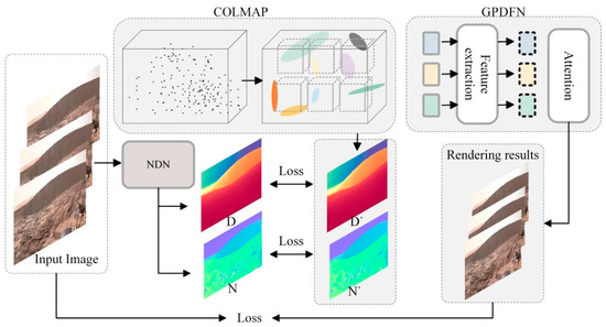
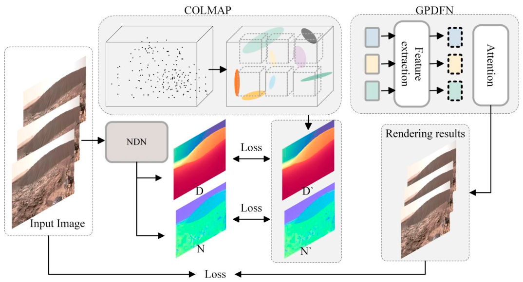
To achieve low-cost digitization of various Martian surface terrains—that is, to perform 3D reconstruction of the corresponding landforms from a sequence of multi-view Martian remote sensing terrain images, obtaining a 3D representation and 2D scene visualization, this study uses the 3DGS algorithm as the basic framework, improves and designs an ESGS algorithm, which improves the geometric accuracy of the algorithm for the extraction of geomorphic texture features, color features, Gaussian position information and three-dimensional reconstruction of Martian landform by adding depth and normal priors. Figure 6 shows the overall framework of the ESGS algorithm.
Figure 6.
The structure of the ESGS model.
The input of ESGS is a sequence of Mars landform images from multiple perspectives, and the output is image data rendered from a three-dimensional Gaussian projection to a two-dimensional plane from the camera perspective. The algorithm consists of two branches. The top branch is the three-dimensional Gaussian parameter learning branch. The Martian surface image sequence is processed using the COLMAP [36] algorithm to generate a sparse point cloud for initializing a three-dimensional Gaussian function. The spherical harmonics, density, quaternion, and other parameters of three-dimensional Gaussians are updated using gradient backpropagation of a neural network, and the rendered image is obtained by projecting three-dimensional Gaussians onto a two-dimensional plane. In three-dimensional space, parameters between adjacent three-dimensional Gaussian functions exhibit a certain degree of correlation. For instance, the spherical harmonic functions and the opacity of neighboring Gaussian functions are similar. When mapped onto a two-dimensional plane, their pixel values should remain close and avoid abrupt jumps. By leveraging this correlation, integrating Gaussian function parameters within a specific range can enhance the fusion of color characteristics, texture features, depth, and normal information on the Martian surface. Ultimately, we can integrate this approach with attention mechanisms to filter noise from the fused information.
The second branch is a three-dimensional Gaussian depth and normal alignment branch. Each time the parameters are updated, the three-dimensional Gaussian depth and normal information are compared with the input depth and normal maps to compute depth and normal losses, guiding the three-dimensional Gaussian function to gradually approach the surface of the Martian landform and improving the three-dimensional reconstruction accuracy of the Martian landform. We trained the NDN network before the 3D reconstruction of the Martian landform and performed only the reasoning step in the ESGS algorithm. To ensure the accuracy of depth and normal priors, we use an open-source outdoor depth and normal supervised learning dataset for training and fine-tune the parameters in the Martian surface scene to enhance the robustness of the NDN network.
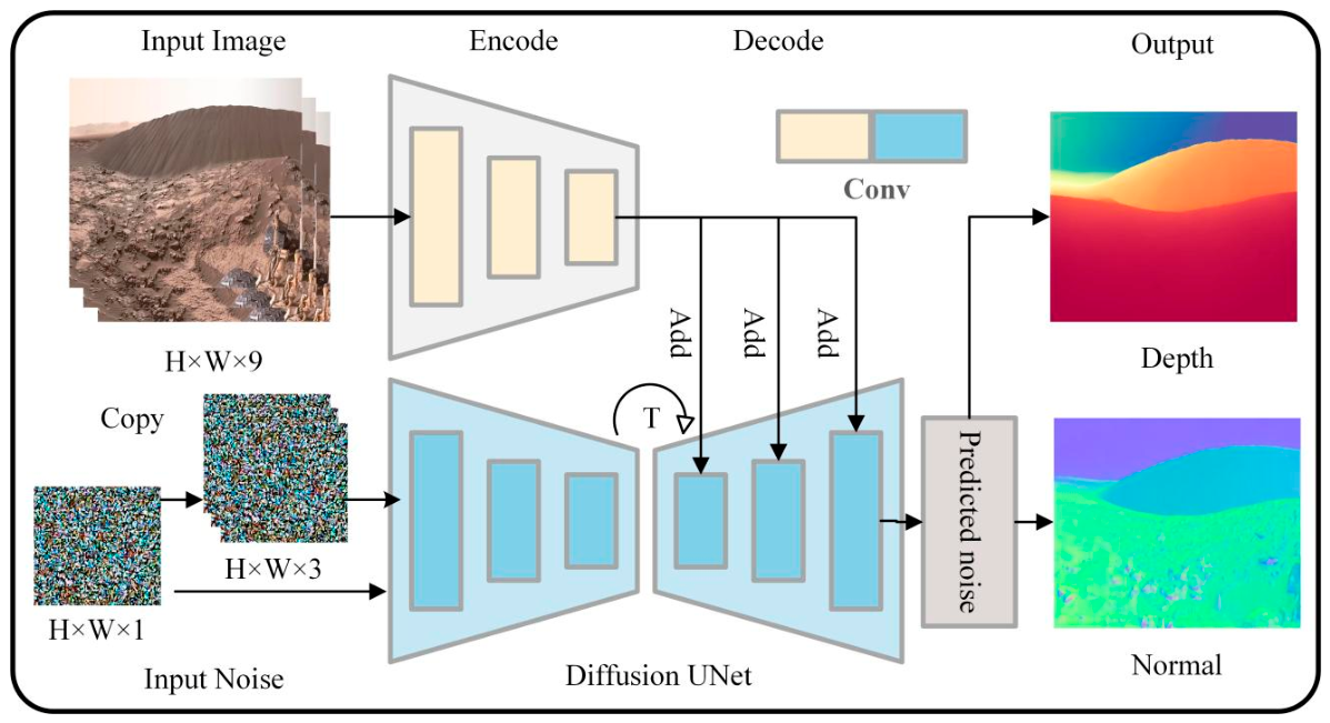
In the ESGS algorithm described above, the two branches—with NDN and GPDFN as their core modules—provide geometric priors and information about the texture and color of neighboring surfaces for the 3D reconstruction of the Martian surface. Specifically, to address the issue that the original 3DGS entirely lacks explicit geometric constraints and produces substantial floating noise in weak-texture regions, this paper designs the NDN network. This network is pre-trained before the 3D reconstruction process and subsequently provides explicit depth and normal priors throughout the optimization. NDN takes multi-view images and random Gaussian noise as joint inputs and synchronously predicts the scene’s depth and normal maps via the reverse denoising process of a diffusion model. Its design follows two key principles: first, it adopts multi-view input rather than single-view prediction, fundamentally avoiding inter-frame geometric inconsistency; second, the output consists of explicit geometric priors, allowing the downstream Gaussian optimizer to flexibly adopt the prior according to the training loss—imposing strong constraints in textureless areas while permitting the rendering loss to dominate optimization in texture-rich regions. On large-scale, continuous terrains on the Martian surface, neighboring 3D Gaussian ellipsoids exhibit strong spatial correlation in parameters such as intensity, color, opacity, and scale. However, the original 3DGS optimizes each Gaussian independently, disrupting this necessary continuity and leading to texture discontinuities and geometric noise in the reconstructed surface. To this end, the GPDFN module enables complementary learning among neighboring Gaussians via cross-voxel feature interactions. First, the Gaussian 3D space is partitioned into a voxel grid, and the parameters of all Gaussians within a single voxel are concatenated into a feature tensor. Then, through a set of learnable spatial position offsets, each voxel is guided to attend to the features of its spatial neighbors, establishing explicit associations among Gaussians. Subsequently, one-dimensional convolution is employed to extract correlation features between Gaussian parameters, which are then weighted and fused via an attention mechanism, ultimately outputting adjusted rendering parameters for each Gaussian. This process ensures that the parameter decision for each Gaussian is no longer isolated but fully incorporates the color, texture, and contextual information of neighboring surfaces. The synergistic cooperation of NDN and GPDFN enhances the geometric accuracy and multi-view consistency of weakly textured Martian terrains. The complete network architecture and detailed analysis of each module are presented in Section 3.3 and Section 3.4, respectively.
3.3. NDN
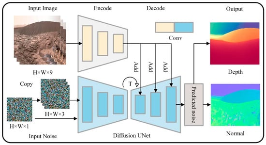
Normal and depth information are very important for the geometric constraints in 3D reconstruction. In this study, we proposed a normal and depth prior estimation network, NDN, based on multi-view images. Before the 3D reconstruction of the Martian surface, the network is pre-trained on the Hypersim and Virtual KITTI datasets. The Hypersim dataset contains 77,400 high-quality indoor scene images, while the Virtual KITTI dataset comprises 21,260 multi-weather outdoor scene images, all of which are annotated with depth and normal labels. Moreover, the NDN restores the normal and depth maps of the Martian surface from random Gaussian noise, using the labeled normal and depth maps as labels for the supervised diffusion model. Figure 7 shows the overall NDN framework.
Figure 7.
The framework of NDN network.
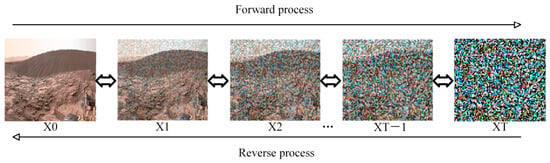
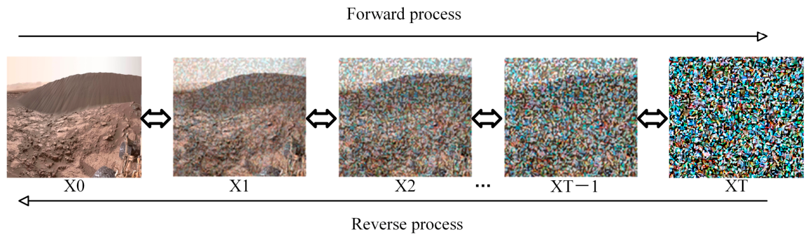
Single-view depth estimation and normal prediction suffer from poor cross-frame view consistency and high prediction variance. The NDN network input is a multi-view (three frames by default) image, with data dimensions of H × W × 9. In addition, there is random Gaussian noise of size H × W, used to recover the depth map and normal map from the noise. In the depth branch, the inter-frame context information is very important for scene depth estimation. In this study, we copy random noise into three channels for fusion with depth and inter-frame context information and extract features from the multi-view image and the noise in the three channels on the subsampling branches. In the depth information upsampling stage, the predicted noise information is fused with the semantic, edge, and contextual information of the Martian surface, thereby improving the diffusion model’s denoising accuracy and enabling better recovery of depth information. In the normal branch, the input is image data and single-channel random noise. Firstly, we fuse the random noise with the image features after downsampling and obtain rough normal information in the first N steps. In the last T-N steps, the normal information containing noise is fused with the semantic information of the image, and the refined normal image is obtained through the diffusion model. In the whole diffusion process, based on the marked normal and depth information, the forward process adds random Gaussian noise at each of the T steps, so that the normal and depth information are completely submerged by noise and almost become random Gaussian noise. In the reverse process, this study uses UNet [37] to predict the Gaussian noise added at each step, and uses the noise added in the forward process as a prior to calculate the loss between the predicted Gaussian noise and the noise added in the forward process. Figure 8 shows the process of recovering image depth and normal information from noise information.
Figure 8.
The process of the diffusion model.
3.4. GPDFN
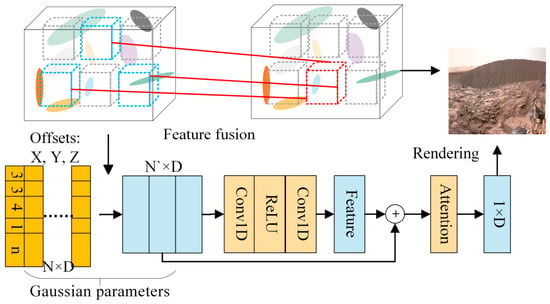
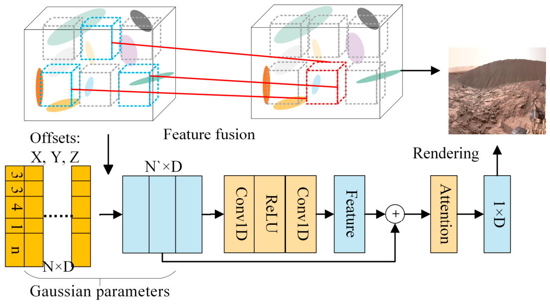
The illumination, density, and other parameters of the three-dimensional Gaussian function at a certain point on the surface of Mars are likely to be affected by the parameters of the surrounding three-dimensional Gaussian function. For example, the direct light and reflection of the light are very similar at different positions in the same area of the three-dimensional scene. To realize complementary learning of multiple Gaussian function parameters, this paper divides the three-dimensional space into voxels and fuses Martian surface color, texture, and contextual information across multiple voxels. Specifically, the parameters of multiple Gaussian functions in a single voxel form a tensor, which is fused with the tensors corresponding to other voxels. The positions of the other voxels can be obtained from a set of learnable spatial position deviations to achieve the fusion of deformable features. Figure 9 shows the network structure of the GPDFN.
Figure 9.
The network structure of the GPDFN.
In three-dimensional space, there are N Gaussian functions, and each Gaussian function contains D parameters, which are the Gaussian position with three values, the scaling factor with three values, the rotation matrix with four values, the opacity with one value, and the spherical harmonic function with n values. Firstly, we establish a close relationship between the Gaussian function and its surrounding Gaussian functions through the learnable offset of the Gaussian function. Secondly, we get N` Gaussian functions from the N Gaussian functions. A 1D convolutional neural network can extract the correlation features of the N` × D-dimensional parameter tensor. Finally, we obtain the corresponding rendering parameters of the Gaussian functions using the attention mechanism, and we obtain the two-dimensional image via raster rendering.
4. Results
4.1. Experimental Environment and Parameter Configuration
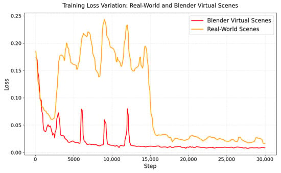
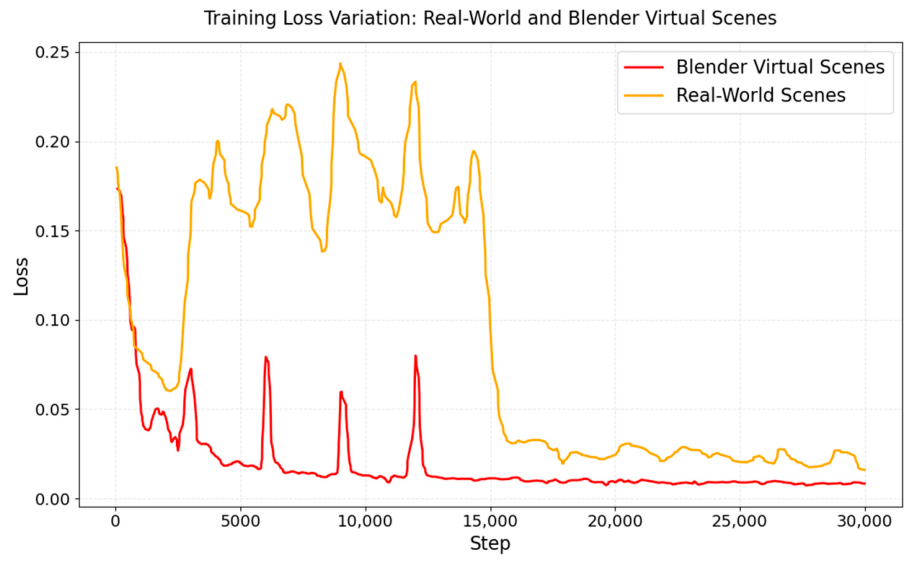
The ESGS algorithm experiment in this paper uses CUDA 11.8, an Intel i7-11700 eight-core CPU, and an NVIDIA GeForce RTX 3090 to build the hardware platform, and selects PyTorch 2.0.0 as the ESGS code development framework. We use the self-built dataset Mars_3D to evaluate the rationality and 3D reconstruction accuracy of this study. The experimental parameters are configured as follows: Densify_from_iter = 500, Densify_until_iter = 15,000, Lr_delay_mul = 0.01, optimizer = Adam, Lr_init = 0.00016, Lr_final = 0.0000016, Max_steps = 30,000, Feature_lr = 0.0025, Lambda_dssim = 0.2, and Densify_grad_threshold = 0.0002. Each algorithm in the comparative experiment trains for 30,000 steps. Due to the sparse perspective of the real scene images, there are fewer images in each scene, and the scene range is extensive, so the loss function fluctuates wildly at the beginning of the training, gradually converges after 15,000 steps, and finally converges around 0.013. After training in the Blender scene, the algorithm converges after 13,000 steps, with a final loss of around 0.007. Figure 10 shows the loss convergence curves of the algorithm in real scenes and Blender virtual scenes from the Mars_3D dataset.
Figure 10.
The loss convergence curves.
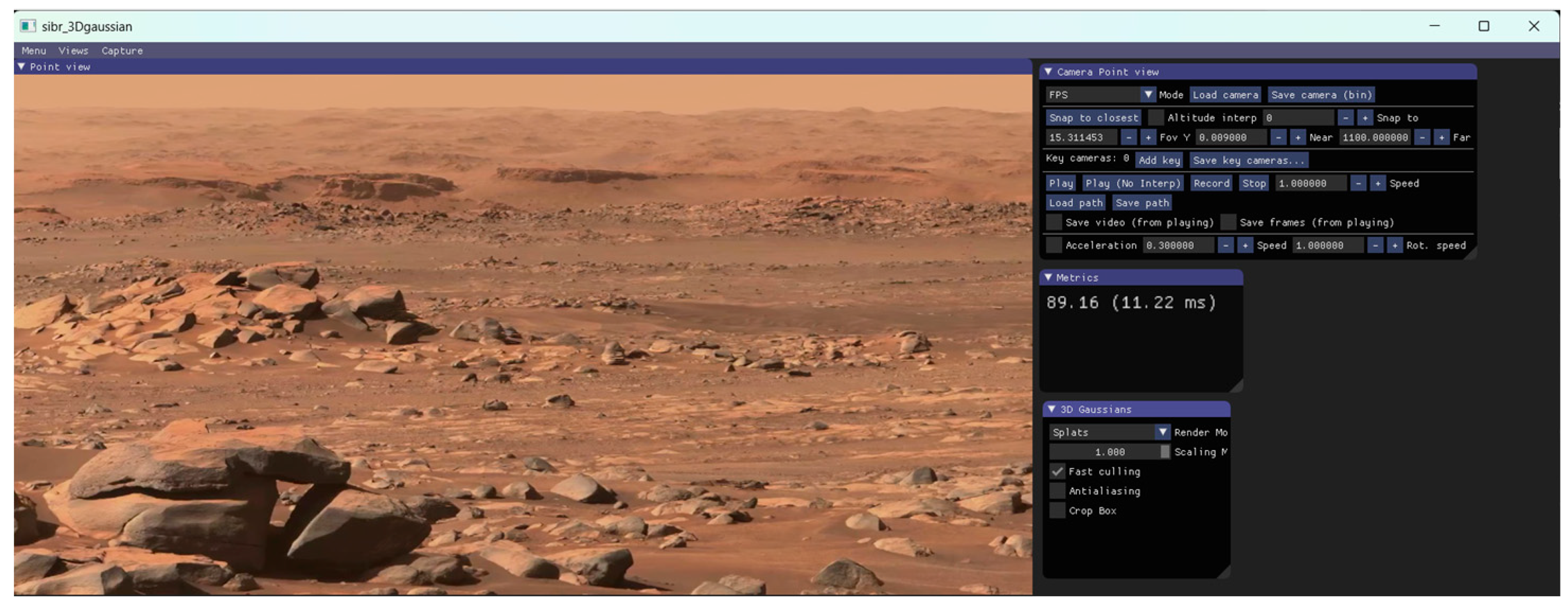
On the Mars_3D dataset, the ESGS algorithm achieves an average training time of 1 h and 15 min per scene, a rendering frame rate of around 90 FPS, and a GPU memory consumption of approximately 16 GB. Figure 11 shows the rendering speed of the training results obtained by ESGS in the 3D rendering software SIBR_gaussianViewer Version 2020.
Figure 11.
The rendering speed of the training results.
4.2. Experimental Indicators
PSNR [38] calculates the mean square error of pixels on all color channels of the image. The higher the value, the better the image reconstruction quality. The formula of PSNR is as follows:
SSIM [39] is an indicator for measuring the similarity between two images across three dimensions: brightness, contrast, and structure. The larger the value, the better. The formula of SSIM is as follows:
LPIPS [40] computes distances between features at different levels. The lower its value, the more similar the two images are perceived to be. The calculation formula of LPIPS is as follows:
4.3. Comparative Experiments on the Mars_3D Dataset
To verify the effectiveness of the algorithm proposed in this paper, we conduct a comparative experiment between the ESGS and 3DGS, DropoutGS [41], Gaussian-DK [42], LITA-GS [43], LongSplat [44], Mip-splatting, PGSR [45], and ScaffoldGS algorithms, and analyze differences in SSIM, PSNR, and LPIPS indicators between the real and rendered images of the Mars landform. Table 1 shows the comparative experimental results of the improved algorithm and the other eight algorithms on the Mars_3D (Real) dataset. Table 2 shows the results of comparative experiments on the Mars_3D (Blender) dataset.
Table 1.
The results of comparative experiments on Mars_3D (Real).
Table 2.
The results of comparative experiments on Mars_3D (Blender).
From the comparative experimental results on the Mars_3D (Real) dataset, we can see that the SSIM of the ESGS is 0.4709, PSNR is 18.90, and LPIPS is 0.419, which is 0.0217 higher than that of the 3DGS; PSNR is reduced by 0.27, and LPIPS is reduced by 0.062. Among the three evaluation indices, two have improved, while PSNR is only slightly reduced. By incorporating the depth and normal prior information into the training, the ESGS algorithm enhances the deep learning network’s ability to extract appearance and texture features of Martian landforms, thereby making the rendered image’s structure and contours more closely match the real scene. The PSNR index focuses more on the pixel differences between the rendered and real images. It shows that ESGS improves the perceptual quality of Martian surface topography by providing depth and normal information, while guiding the spatial position of the three-dimensional Gaussians to change, resulting in weak changes in a small number of rendered pixels and thereby reducing the PSNR.
On the whole, the index’s decline is acceptable. The PSNR of ESGS is still higher than that of the other seven algorithms. The Martian landform contains many high-frequency details. The PSNR index should not be over-optimized; otherwise, a higher PSNR will introduce a visual smoothing effect to the Martian landform.
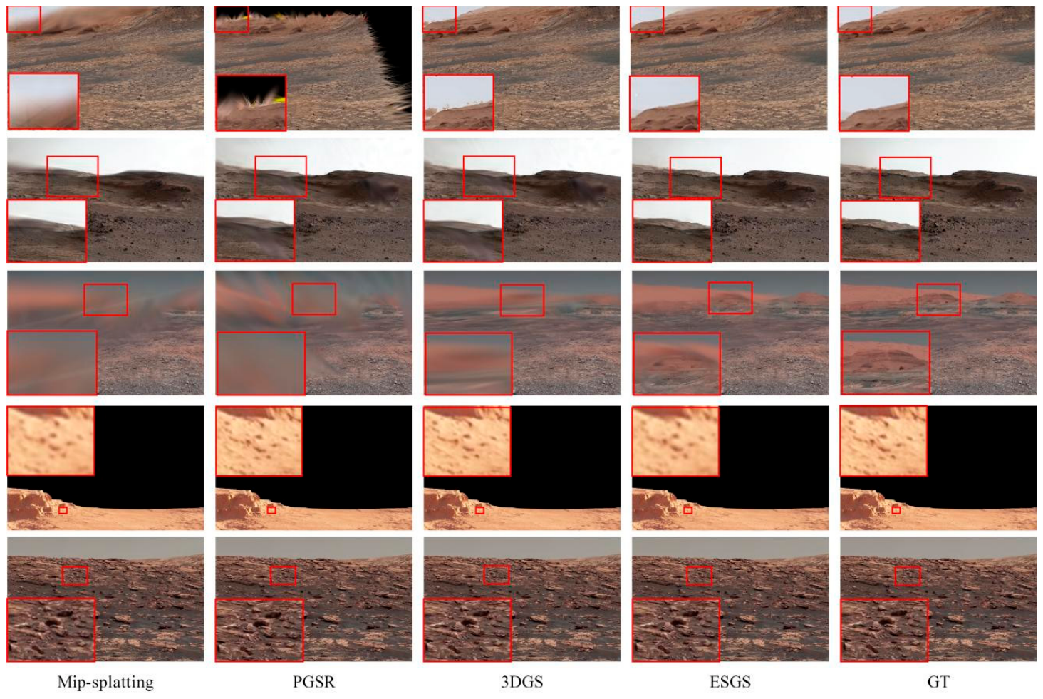
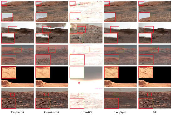
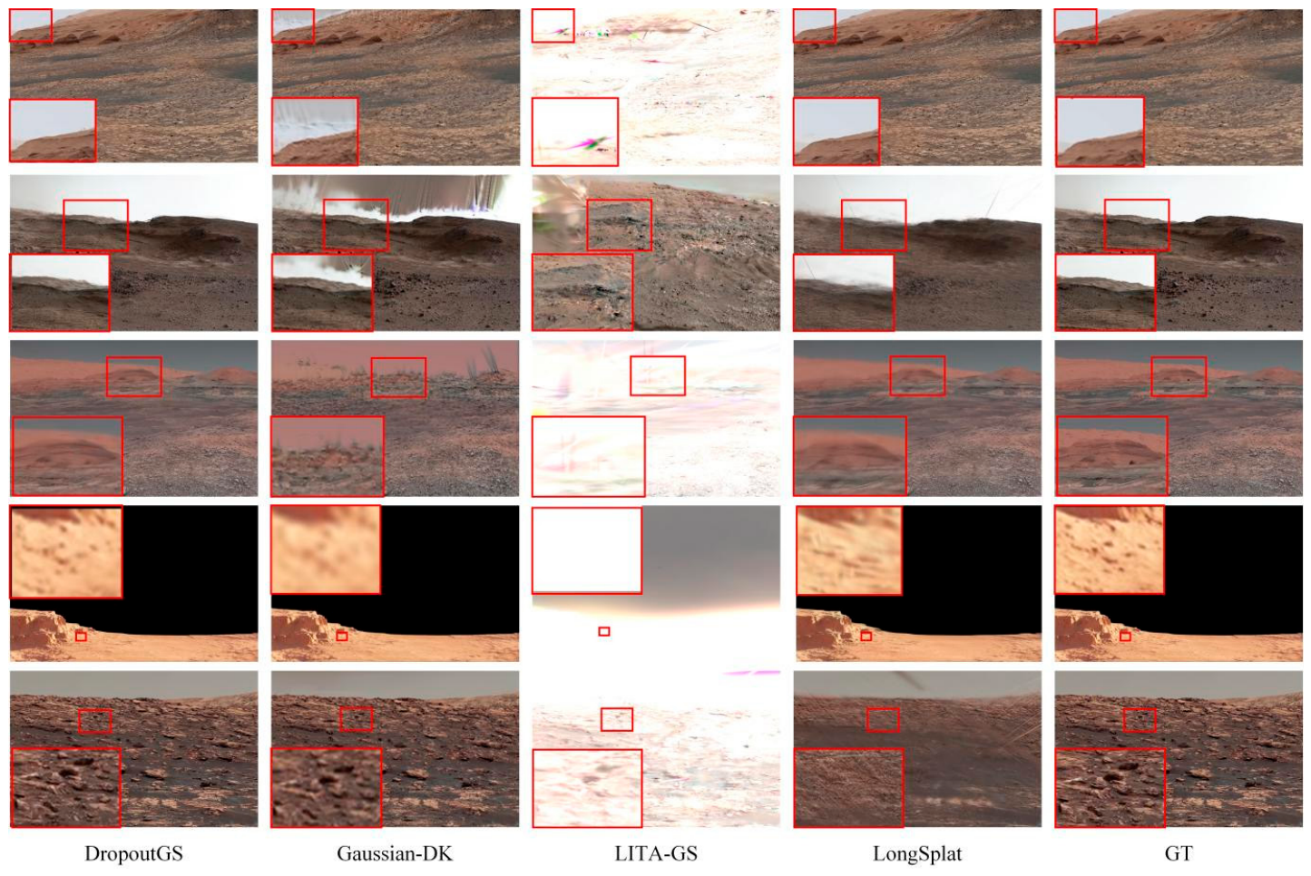
Observing the results of comparative experiments on Mars_3D (Blender), we can find that due to the rich perspective of images in the virtual scene, each scene has 30 images, and the details of the Martian surface topography texture generated by Blender are less than those of the real scene, so the final results of 3D reconstruction of Martian topography have been improved as a whole. The SSIM of the ESGS algorithm is 0.9182, the PSNR is 27.89, and the LPIPS is 0.086, which is similar to the results of comparative experiments on Mars_3D (Real). The SSIM and LPIPS scores of our algorithm are optimal, and the PSNR is slightly lower, yet it is still better than those of the other seven algorithms. On the other hand, we can evaluate the improvement of the ESGS algorithm by comparing the rendering results of the Martian landform produced by different algorithms. We selected four optimal algorithms to compare the rendering quality of Martian landforms: Mip-splatting, PGSR, 3DGS, and ESGS. Figure 12 shows the comparison results of the comparative experiment. Figure 13 shows the comparison results of other algorithms.
Figure 12.
The render results of the comparative experiment (Mars_3D). The red boxes highlight magnified texture details in local regions of the rendering results.
Figure 13.
The render results of the other algorithms (Mars_3D). The red boxes highlight magnified texture details in local regions of the rendering results.
According to comparative experimental results, because the ESGS algorithm is supported by depth and normal prior information, its results are more in line with the actual landform texture in medium- to long-distance rendering of Martian surface landforms, with fewer noise artifacts and burrs. For example, the effect of ESGS will be greater in the first and third lines. In some close-up locations, the performance of various algorithms on the Martian landform texture differs slightly, mainly in how they present detailed textures. For example, in the fourth- and fifth-row scenes, the ESGS performs better at pixel-level color rendering and overall scene rendering of the Martian landform.
The renderings produced by other algorithms are far worse than those of the four algorithms above. There are many noise artifacts and burrs in the Martian landform scene. For example, the scene in the first three lines of the rendering results differs significantly from the GT. Due to the limited number of multi-view images in most Martian landform scenes, the LITA-GS did not learn the light compensation feature well, leading to a severe overexposure in the rendering results. Overall, the ESGS’s rendering results were the best.
4.4. Comparative Experiments on the Sora Dataset
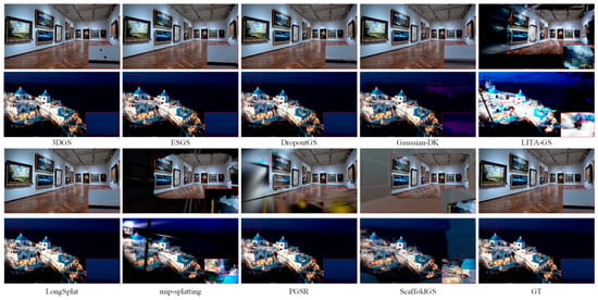
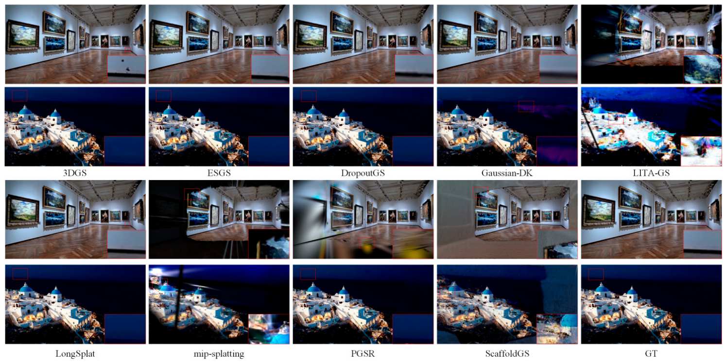
To validate the robustness of the proposed ESGS algorithm and demonstrate that the improved algorithm remains effective on other datasets, this subsection compares ESGS with 3DGS, DropoutGS, Gaussian-DK, LITA-GS, LongSplat, Mip-splatting, PGSR, and ScaffoldGS. Figure 14 shows the rendering results of these algorithms on the Sora 3D reconstruction dataset.
Figure 14.
The rendering results on the Sora dataset. The red boxes highlight magnified texture details in local regions of the rendering results.
Based on the rendering results, the ESGS algorithm achieves superior rendering quality on the Sora dataset, yielding smaller errors relative to the ground truth. At junctions such as those between the ground and sky or between different walls, it rarely produces noise or artifacts, and no large-scale rendering distortions or color shifts are observed. In contrast, Gaussian-DK, LITA-GS, Mip-splatting, PGSR, and ScaffoldGS all exhibit severe rendering distortion, Gaussian parameter degradation, and blurred artifacts. 3DGS produces local noise at planar boundaries. Table 3 shows the reconstruction metrics of all algorithms.
Table 3.
The results of comparative experiments on the Sora dataset.
According to the reconstruction results listed in Table 3, the proposed method achieves an SSIM of 0.8653, a PSNR of 25.87 dB, and an LPIPS of 0.082, outperforming 3DGS by 0.0081, 0.55 dB, and 0.053, respectively. Compared with Gaussian-DK, LITA-GS, LongSplat, Mip-splatting, PGSR, ScaffoldGS, and DropoutGS, its SSIM is higher by 0.0419, 0.2194, 0.0051, 0.1832, 0.069, 0.1576, and 0.0075, respectively. ESGS attains the best SSIM, PSNR, and LPIPS values, demonstrating stronger 3D scene reconstruction capability, enhanced geometric feature extraction, and better generalization.
4.5. Ablation Experiment
The NDN network designed in this paper provides the ESGS with the depth and normal prior information of Martian landforms. To verify whether depth and normal information serve as positive guiding signals, this section examines their impact on the ESGS algorithm. Table 4 shows the ablation experimental results for the ESGS.
Table 4.
The results of ablation experiment on the Mars_3D.
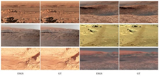
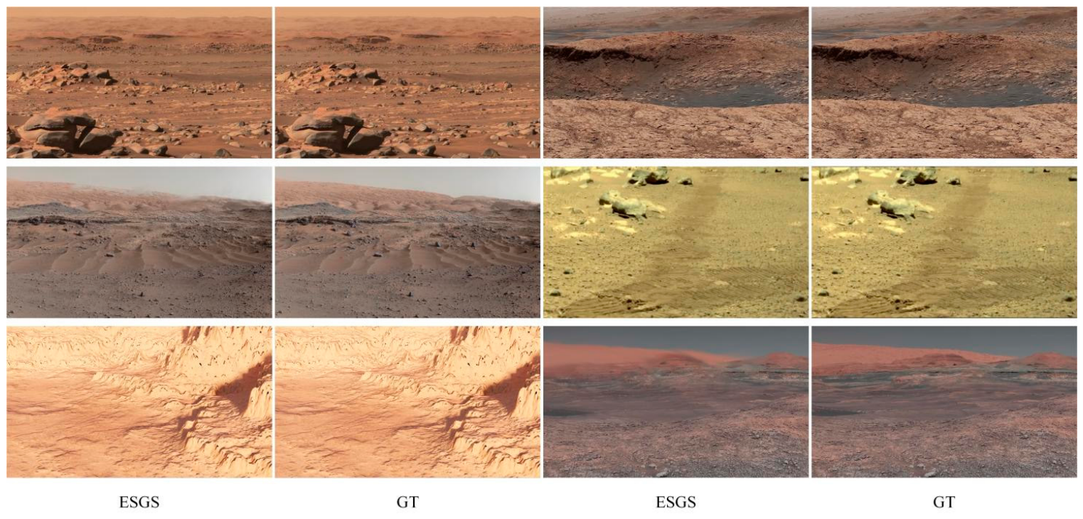
According to the ablation experiment results, both depth and normal information can improve the accuracy of the 3D reconstruction of Martian landforms. Under certain conditions, the local gradient of the depth value can estimate the normal information of the scene surface, so using a single type of information alone can also improve results. When using both types of information simultaneously, the 3D reconstruction effect of ESGS is better. The average SSIM on the Mars_3D dataset is 0.6834, the average PSNR is 23.72, and the average LPIPS is 0.261. After adding the GPDFN, the 3D reconstruction effect of the ESGS was the best, with an SSIM of 0.6946, PSNR of 23.40, and LPIPS of 0.253. Figure 15 shows the ESGS rendering results on the Mars_3D dataset.
Figure 15.
The rendering results of the ESGS.
Furthermore, ablation studies were conducted on the Sora dataset to validate the effectiveness of the NDN network and GPDFN. Table 5 shows the ablation results on the Sora dataset.
Table 5.
The results of ablation experiment on the Sora dataset.
As shown in Table 5, when the NDN network uses only depth or normal information on the Sora dataset, the ESGS algorithm achieves SSIM scores of 0.8607 and 0.8585, respectively, representing improvements of 0.0035 and 0.0013 over 3DGS. Depth information, normal information, and GPDFN all enhance ESGS’s 3D information-extraction capabilities. When all three modules are used together, the algorithm achieves the best 3D reconstruction performance, with an SSIM of 0.8653, a PSNR of 25.87 dB, and an LPIPS of 0.082.
4.6. Visualization Experiments of the ESGS
4.6.1. Point Cloud Visualization
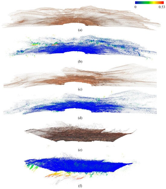
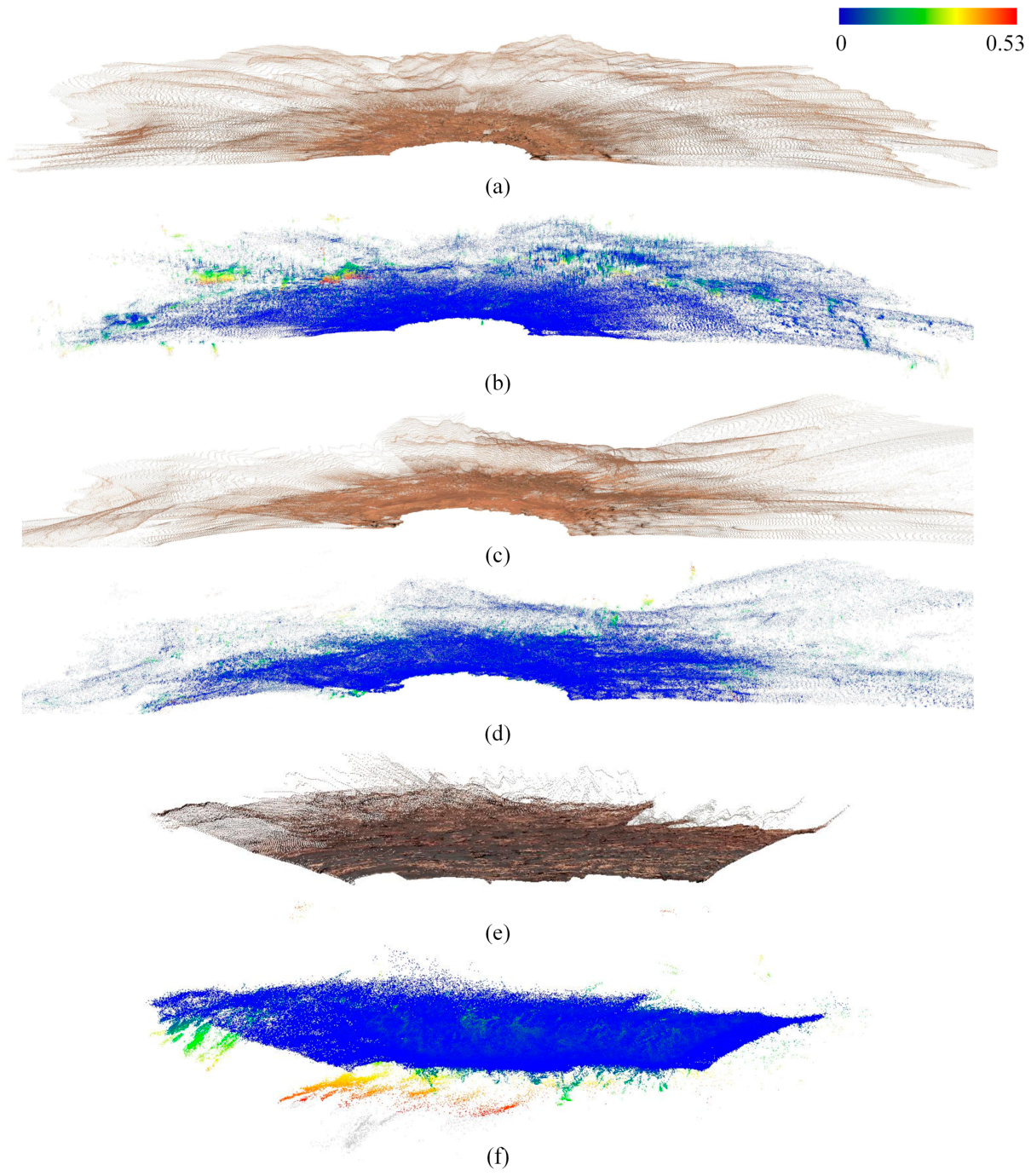
To verify the feasibility of the proposed algorithm for 3D reconstruction of the Martian surface using remote sensing image sequences, this subsection presents difference heatmaps [46,47] between the ground-truth point clouds of the Mars_3D dataset and the reconstructed point clouds obtained after ESGS training. The heatmap transitions gradually from dark blue to dark red, with cool colors indicating regions with small differences and warm colors indicating regions with large differences. These difference heatmaps can effectively illustrate the overall degree of deviation between the reconstructed point cloud and the true geometry and indirectly reflect the fitting performance of the Gaussian parameters. We selected three 3D scenes generated from Martian surface remote sensing images, with varying reconstruction quality, which can accurately represent the overall reconstruction issues. The point cloud difference maps for the 3D reconstruction of the Martian surface are shown in Figure 16.
Figure 16.
Point cloud difference maps for 3D reconstruction of the Martian surface. (a) Point cloud ground truth of Scene 0. (b) Difference heatmap between ground-truth and reconstructed point cloud of Scene 0. (c) Point cloud ground truth of Scene 1. (d) Difference heatmap between ground-truth and reconstructed point cloud of Scene 1. (e) Point cloud ground truth of Scene 2. (f) Difference heatmap between ground-truth and reconstructed point cloud of Scene 2.
From Figure 16, it can be observed that for Scene 0, the difference between the reconstructed point cloud and the ground truth gradually increases at medium and long ranges. In contrast, in the region of the Martian surface closer to the camera, the difference remains within an acceptable range, consistent with the inference that the introduced geometric prior achieves higher accuracy at closer distances. For Scene 1, clusters of point clouds with large differences appear at the boundary between the Martian surface and the sky, which can readily give rise to Gaussian artifacts. For Scene 2, the reconstructed point cloud exhibits the largest deviation from the ground truth. To accurately fit the fine textures of the Martian surface scene, a large number of discrete Gaussians were split beneath the surface during training to compensate for pixel-wise differences between the rendered and input images. Although this improved the reconstruction metrics, it reduced the consistency of the 3D Martian surface scene and increased Gaussian redundancy.
Furthermore, to verify the effectiveness of the ESGS algorithm in improving the geometric accuracy of 3D reconstruction of the Martian surface, we compared distance errors between the input point clouds and those obtained after training, where the input point clouds were used only during Gaussian initialization. Table 6 shows the reconstruction point cloud errors of different algorithms on the Mars_3D dataset. The mean distances and standard deviations reported in Table 6 are the averaged results for the real and Blender scenes in the Mars_3D dataset. It should be noted that point clouds of real scenes, which are not measured by instruments such as LiDAR, do not accurately reflect the geometric structure of the Martian surface; therefore, these results cannot directly demonstrate the improvement in geometric reconstruction accuracy achieved by the ESGS algorithm. Nevertheless, they serve to validate the ESGS algorithm’s transfer capability for reconstructing from non-realistic to realistic Martian surface geometries, thereby indirectly demonstrating the algorithm’s effectiveness and stability in enhancing geometric reconstruction accuracy.
Table 6.
Reconstruction point cloud errors for different algorithms on the Mars_3D dataset.
We used CloudCompare to load the input and reconstructed point clouds separately, then used its distance-computation tool to obtain 3D Euclidean distances. By examining the point cloud error data of each algorithm, it can be observed that in the task of Martian surface 3D reconstruction, the ESGS algorithm achieves the smallest mean distance error of 0.0097 and the smallest standard deviation of 0.0205. This demonstrates that the geometric priors provided by ESGS effectively reduce the number of floating Gaussians in weak-texture regions detached from the Martian surface. The low standard deviation also reflects that the GPDFN can promote parameter fusion among neighboring Gaussians, thereby enhancing the global stability of the 3D reconstruction of the Martian surface.
Furthermore, the Martian surface structures generated in Blender include ground-truth geometric data that can be accessed directly within Blender. To provide more compelling evidence supporting the conclusion that our ESGS algorithm can improve the geometric accuracy of 3D reconstruction of the Martian surface, we compared each algorithm on the Mars_3D (Blender) dataset in terms of the mean errors and standard deviations between the input point clouds and the point clouds obtained after training. The results are presented in Table 7.
Table 7.
Reconstruction point cloud errors for different algorithms on the Mars_3D (Blender) dataset.
Once again, we loaded the point clouds generated from the ground-truth geometric data and those reconstructed by the ESGS algorithm into CloudCompare 2.14.beta software to compute the mean distance error and standard deviation between them. The data indicate that the ESGS algorithm achieves the smallest mean distance error and standard deviation in real geometric scenes among all compared methods, with values of 0.0089 and 0.0195, respectively. This confirms the effectiveness of the ESGS algorithm in enhancing geometric accuracy for the 3D reconstruction of the Martian surface.
4.6.2. Training Visualization
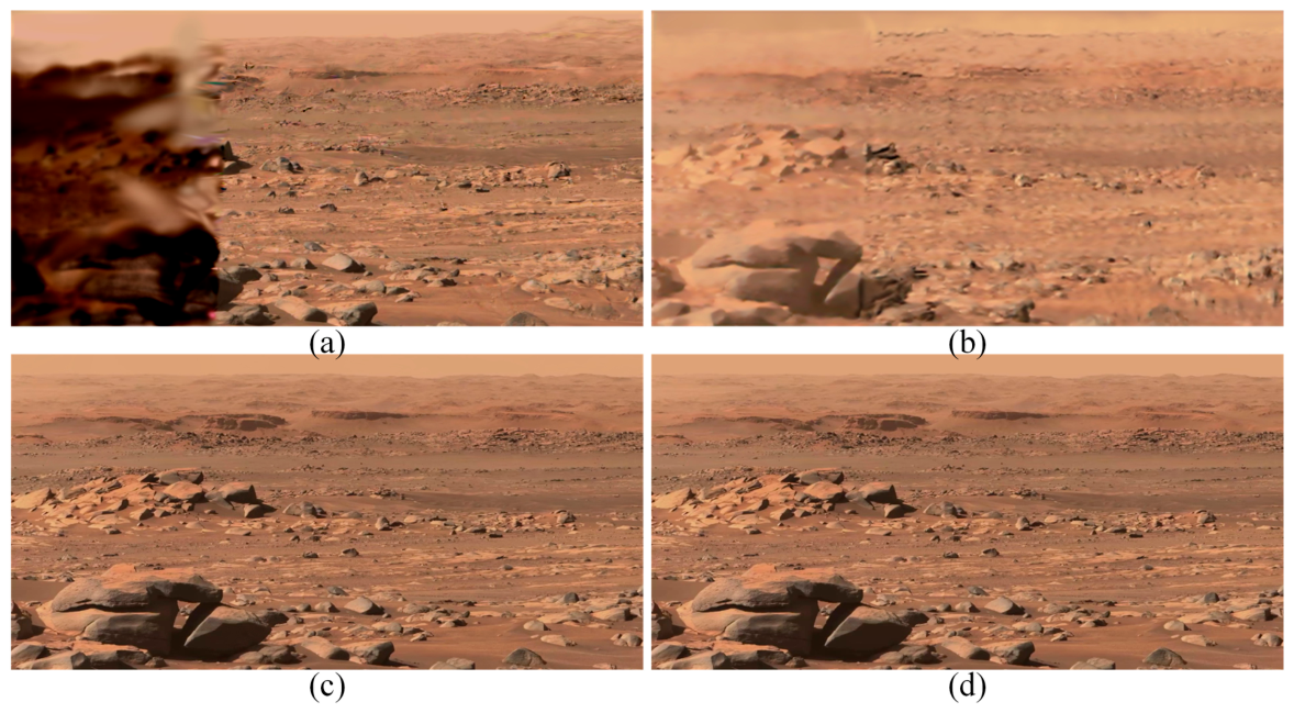
To verify the usability of the Mars_3D dataset and the effectiveness of the proposed ESGS algorithm, we recorded the evolution of the 3D reconstructed Martian surface scenes from blurry to clear as the training epochs increased. Finally, the rendered images of the trained 3D scenes from the camera viewpoint are presented in Figure 17.
Figure 17.
Rendering results of the ESGS training process. (a) Rendering result at epoch 7000. (b) Rendering result at epoch 15,000. (c) Rendering result at epoch 30,000. (d) Ground-truth image.
From the training results, as the number of training epochs increases, the ESGS algorithm’s fitting degree to 3D Martian surface scenes gradually improves, with scene details becoming richer. Ultimately, the training result at epoch 30,000 is almost indistinguishable from the real input image.
4.7. Validity Analysis of Prior Information
To clarify whether the improved 3D reconstruction accuracy of the Martian surface achieved by incorporating the NDN network into the ESGS algorithm is attributable to the diffusion model itself or to the introduced prior information, a set of comparative experiments is designed in this subsection. The Depth Anything and Metric3D algorithms are employed to provide depth priors for the Martian surface, and Table 8 shows the 3D reconstruction results obtained using each algorithm.
Table 8.
3D reconstruction results of the Martian surface after using different networks.
Based on the impact of incorporating different prior information on the Martian surface 3D reconstruction results in the ESGS algorithm, it can be observed that reconstruction accuracy improves when depth or normal priors are added, without requiring a diffusion model. This indirectly demonstrates the necessity and effectiveness of the depth and normal priors provided by the NDN network within the ESGS algorithm.
4.8. Analysis of Fusion Settings in GPDFN
In the GPDFN, we perform fusion learning on the parameters of adjacent Gaussians, thereby introducing local contextual information of the Martian surface scene. This approach can expand the network’s receptive field, maintain the continuity of the Martian surface, and reduce Gaussian artifacts caused by sparse viewpoints. As the number of fused Gaussians gradually increases, the Martian surface reconstruction results of the ESGS algorithm with GPDFN are presented in Table 9.
Table 9.
Comparative experimental results with different numbers of Gaussians.
As shown in Table 9, with increasing the number of fused Gaussians, the overall 3D reconstruction accuracy of ESGS first increases and then decreases, achieving the best accuracy at three fused Gaussians, with SSIM improved by 0.0107 compared to the case without fusion. The number of fused Gaussians is a critical hyperparameter that must be tuned based on the scene’s Gaussian density, surface roughness, and viewpoint sparsity. In Martian terrain data, where real viewpoints are relatively sparse, large-scale fusion can overly rely on neighborhood priors, thereby suppressing the ability to learn unique details from actual observations and making the model more inclined to generate smooth surfaces. However, the random distribution of rocks in actual Martian landforms does not satisfy the assumption of large-scale surface smoothness.
5. Discussion
Figure 15 shows the rendering results of the ESGS under six scenarios of Martian landforms. According to the observation, if the landform where the training perspective has a sky background, the depth and normal information of Martian landforms provided by the NDN network is inaccurate at the junction of sky and landform, resulting in a large number of noise artifacts at the junction, and the rendering effect is inconsistent with the actual image (the first scene on the second line and the second scene on the third line in the figure). According to calculations performed using the point cloud distance error measurement tool in CloudCompare, at the boundary between the Martian surface and the sky, as well as in distant regions, the average point cloud error is 0.283, which is considerably higher than the mean error between the input and reconstructed point clouds. In the medium- and short-range Martian landscape scene, the ESGS rendering results are almost identical to the real image, and the subtle differences are difficult to distinguish by eye. The ESGS can be applied to the three-dimensional reconstruction of Martian and other landscapes.
Based on the above experiments, the ESGS has demonstrated excellent performance in 3D reconstruction of the Martian surface. During the research, we also identified some limitations and problems. First, there are few datasets for the 3D reconstruction of the Martian surface. We generate the Martian surface dataset (Mars_3D) with nine scenes using remote sensing images from NASA. However, the dataset’s real-world scenes are very sparse, making 3D reconstruction of the Martian surface difficult and prone to overfitting. The 3D reconstruction of the Martian surface outside the field of view is poor, and the reconstruction quality cannot be evaluated. Secondly, if there are sky and other background elements in the Martian surface image, they can easily lead to errors in depth and normal information, thereby reducing the quality of the landscape’s three-dimensional reconstruction. In future work, it is necessary to add a mask for sky pixels, ignore the influence of the sky and other backgrounds in the calculation process, and further improve the depth and normal a priori accuracy.
In addition, the GPDFN uses the surrounding Gaussian parameters as a feature supplement, introduces the pixel smoothing effect in the rendering results, and combines the depth or normal information to guide the spatial position of the three-dimensional Gaussian, resulting in some pixels with weak pixel value changes, which ultimately leads to the reduction of the PSNR index. Considering the above problems, we will collect Martian surface images from other scenes to ensure the availability of multi-view images, thereby facilitating further study of the digital reconstruction of the Martian surface.
6. Conclusions
Because there are many rocks, craters, steep slopes, and sandy terrain on the Martian surface, the surface texture and structure are complex, and there is no support for depth or normal information, it is difficult to ensure geometric consistency between the reconstructed and real scenes. To solve these problems, this paper proposes the ESGS algorithm, which provides geometric prior information about the scene via the NDN network, thereby facilitating the extraction of color, texture, and inter-frame context information of the Martian surface. The GPDFN fuses multi-Gaussian-correspondence feature information, improving the algorithm’s accuracy in three-dimensional reconstruction of the Martian surface. The effectiveness of the algorithm is demonstrated through comparative and ablation experiments on the self-built dataset (Mars_3D) and the Sora dataset. On Martian scenes, ESGS achieves an SSIM of 0.6946, a PSNR of 23.40, and an LPIPS of 0.253. Compared with the baseline model, ESGS improves SSIM by 0.0146, while PSNR and LPIPS decrease by 0.67 and 0.034, respectively. On the Sora scenes, ESGS achieves an SSIM of 0.8653, a PSNR of 25.87, and an LPIPS of 0.082. Compared with the baseline model, ESGS improves SSIM by 0.0081 and PSNR by 0.55, while LPIPS decreases by 0.053. In future work, we will continue to improve the ESGS algorithm to address inaccuracies in depth and normal information at long distances on the Martian surface and noise artifacts at the junction of geomorphology and sky and to provide a set of feasible schemes for the digital reconstruction of the Martian surface.
Author Contributions
Conceptualization, Q.G. and Y.L. (Yang Li); methodology, Q.G. and Y.L. (Ying Liu); software, Q.G. and G.L.; formal analysis, L.C.; writing—original draft preparation, Q.G.; writing—review and editing, L.C. and Y.L. (Yang Li). All authors have read and agreed to the published version of the manuscript.
Funding
This work is supported by the Department of Science and Technology of Jilin Province, China [20230203028SF].
Data Availability Statement
The self-constructed Mars_3D dataset in this study is available at the following GitHub link: https://github.com/LG973641114/ESGS.git (accessed on 27 June 2026). The Sora 3D reconstruction dataset can be obtained from [35].
Acknowledgments
The authors would like to thank the editors and the anonymous reviewers for their valuable comments and for greatly improving our manuscript.
Conflicts of Interest
The authors declare no conflicts of interest.
Abbreviations
The following abbreviations are used in this manuscript:
| ESGS | Enhanced Surface Geometric Accuracy method based on 3DGS |
| NDN | Normal and depth prior estimation network |
| 3DGS | 3D Gaussian splatting |
| GPDFN | Gaussian parameter-based deformable fusion network |
| 3D | Three Dimensional |
| SSIM | Structural Similarity Index Measure |
| PSNR | Peak Signal-to-Noise Ratio |
| LPIPS | Learned Perceptual Image Patch Similarity |
| SFM | Structure from Motion |
| FPS | Frames Per Second |
| NASA | National Aeronautics and Space Administration |
| Conv | Convolution |
| GT | Ground truth |
| Adam | Adaptive Moment Estimation |
References
- Zang, P.; He, J.; Yang, Y.; Li, Y.; Zhang, H. Enhanced RT-DETR with Dynamic Cropping and Legendre Polynomial Decomposition Rockfall Detection on the Moon and Mars. Remote Sens. 2025, 17, 2252. [Google Scholar] [CrossRef] [Scilit]
- He, H.; Wu, Z.; Rong, Z.; He, F.; Cheng, X.; Wang, Y.; Gao, J.; Wei, Y. The Evolution of the Mars Year (MY) 35 Anomalous Spring Dust Storm and Its Influence on the Chryse and Utopia Plains. Remote Sens. 2025, 17, 3542. [Google Scholar] [CrossRef] [Scilit]
- Wang, Y.; Zhou, S.; Yan, T.; Guo, S.; Chen, Z.; He, Y.; Lu, Y. A Dual-Channel Passive Limb Imaging System (DUALIS) for Mars with UV Airglow-Based CO2 Retrieval and 557.7 nm Doppler Wind Imaging Interferometry. Remote Sens. 2026, 18, 731. [Google Scholar] [CrossRef] [Scilit]
- Yang, C.; Wu, Y.; Zhao, H.; Zhao, M. Transformer-Based Multi-Modal Fusion for Martian Impact Crater Classification. Remote Sens. 2026, 18, 599. [Google Scholar] [CrossRef] [Scilit]
- Li, J.; Chen, B.; Li, T.; Wu, Z.; Zong, W. Seasonal and Interannual Variation in Martian Gravity Waves at Different Altitudes from the Mars Climate Sounder. Remote Sens. 2026, 18, 319. [Google Scholar] [CrossRef] [Scilit]
- Huang, W.; Cao, H.; Xin, Y.; Liu, C.; Cui, J.; Zhao, Y.; Xue, B.; Ling, Z. Compositional and Mineralogical Diversity of Jezero Western Fan, Mars, Revealed by Elemental Observations. Remote Sens. 2026, 18, 140. [Google Scholar] [CrossRef] [Scilit]
- Chen, Z.; Wu, B.; Liu, W.C. Mars3DNet: CNN-Based High-Resolution 3D Reconstruction of the Martian Surface from Single Images. Remote Sens. 2021, 13, 839. [Google Scholar] [CrossRef] [Scilit]
- Cao, J.; Huang, R.; Xu, Y.; Ye, Z.; Qian, J.; Hoegner, L.; Tong, X. LoGAN: A novel local attentive generative adversarial resizable network for detailed 3D reconstruction of the Martian surface using monocular HiRISE images and DTMs. ISPRS J. Photogramm. Remote Sens. 2025, 225, 302–327. [Google Scholar] [CrossRef] [Scilit]
- Zou, Z.; Zhou, Y.; Li, C.; Dong, Z. PFMGAN: A Generative Adversarial Network with Physics Fusion for DTM Generation from Martian Monocular Images. Remote Sens. 2026, 18, 1354. [Google Scholar] [CrossRef] [Scilit]
- Kerbl, B.; Kopanas, G.; Leimkuehler, T.; Drettakis, G. 3D Gaussian splatting for real-time radiance field rendering. ACM Trans. Graph. 2023, 42, 139:1–139:14. [Google Scholar] [CrossRef] [Scilit]
- Nyimbili, P.H.; Demirel, H.; Seker, D.Z.; Erden, T. Structure from motion (sfm)-approaches and applications. In Proceedings of the International Scientific Conference on Applied Sciences, Antalya, Turkey, 27–30 September 2016; pp. 27–30. [Google Scholar]
- Seeley, R.T. Spherical harmonics. Am. Math. Mon. 1966, 73, 115–121. [Google Scholar] [CrossRef] [Scilit]
- Mildenhall, B.; Srinivasan, P.P.; Tancik, M.; Barron, J.T.; Ramamoorthi, R.; Ng, R. Nerf: Representing scenes as neural radiance fields for view synthesis. Commun. ACM 2021, 65, 99–106. [Google Scholar] [CrossRef] [Scilit]
- Huang, B.; Yu, Z.; Chen, A.; Geiger, A.; Gao, S. 2d gaussian splatting for geometrically accurate radiance fields. In ACM SIGGRAPH 2024 Conference Papers; Association for Computing Machinery: New York, NY, USA, 2024; pp. 1–11. [Google Scholar]
- Lu, T.; Yu, M.; Xu, L.; Xiangli, Y.; Wang, L.; Lin, D.; Dai, B. Scaffold-gs: Structured 3d gaussians for view-adaptive rendering. In Proceedings of the IEEE/CVF Conference on Computer Vision and Pattern Recognition, Seattle, WA, USA, 16–22 June 2024; pp. 20654–20664. [Google Scholar]
- Yu, Z.; Chen, A.; Huang, B.; Sattler, T.; Geiger, A. Mip-splatting: Alias-free 3d gaussian splatting. In Proceedings of the IEEE/CVF Conference on Computer Vision and Pattern Recognition, Seattle, WA, USA, 16–22 June 2024; pp. 19447–19456. [Google Scholar]
- Wu, G.; Yi, T.; Fang, J.; Xie, L.; Zhang, X.; Wei, W.; Wang, X. 4d gaussian splatting for real-time dynamic scene rendering. In Proceedings of the IEEE/CVF Conference on Computer Vision and Pattern Recognition, Seattle, WA, USA, 16–22 June 2024; pp. 20310–20320. [Google Scholar]
- Yuan, Y.; Shen, Q.; Yang, X.; Wang, X. 1000+ fps 4d gaussian splatting for dynamic scene rendering. In Proceedings of the Thirty-ninth Annual Conference on Neural Information Processing Systems, San Diego, CA, USA, 20 March 2025. [Google Scholar]
- Peng, C.; Zhang, C.; Wang, Y.; Xu, C.; Xie, Y.; Zheng, W.; Zhan, W. Desire-gs: 4d street gaussians for static-dynamic decomposition and surface reconstruction for urban driving scenes. In Proceedings of the Computer Vision and Pattern Recognition Conference, Nashville, TN, USA, 24–28 June 2025; pp. 6782–6791. [Google Scholar]
- Zhou, H.; Shao, J.; Xu, L.; Bai, D.; Qiu, W.; Liu, B.; Liao, Y. Hugs: Holistic urban 3d scene understanding via gaussian splatting. In Proceedings of the IEEE/CVF Conference on Computer Vision and Pattern Recognition, Seattle, WA, USA, 16–22 June 2024; pp. 21336–21345. [Google Scholar]
- Chen, Y.; Gu, C.; Jiang, J.; Zhu, X.; Zhang, L. Periodic vibration gaussian: Dynamic urban scene reconstruction and real-time rendering. arXiv 2023, arXiv:2311.18561. [Google Scholar]
- Yan, Y.; Lin, H.; Zhou, C.; Wang, W.; Sun, H.; Zhan, K.; Peng, S. Street gaussians: Modeling dynamic urban scenes with gaussian splatting. In European Conference on Computer Vision; Springer Nature: Cham, Switzerland, 2024; pp. 156–173. [Google Scholar]
- Peng, J.; Chen, C.; Liu, Y. F2Plenoxels: Fast voxel radiance fields without neural networks for few-shot view synthesis. J. King Saud Univ. Comput. Inf. Sci. 2026, 38, 98. [Google Scholar] [CrossRef] [Scilit]
- Zhou, X.; Lin, Z.; Shan, X.; Wang, Y.; Sun, D.; Yang, M.H. Drivinggaussian: Composite gaussian splatting for surrounding dynamic autonomous driving scenes. In Proceedings of the IEEE/CVF Conference on Computer Vision and Pattern Recognition, Seattle, WA, USA, 16–22 June 2024; pp. 21634–21643. [Google Scholar]
- Lo, K.S.H.; Peters, J. Diff-DEM: A diffusion probabilistic approach to digital elevation model void filling. IEEE Geosci. Remote Sens. Lett. 2024, 21, 1–5. [Google Scholar] [CrossRef] [Scilit]
- Ho, J.; Jain, A.; Abbeel, P. Denoising diffusion probabilistic models. Adv. Neural Inf. Process. Syst. 2020, 33, 6840–6851. [Google Scholar]
- Zhao, J.; Yuan, Y.; Dong, Y.; Li, Y.; Shao, C.; Yang, H. Void filling of digital elevation models based on terrain feature-guided diffusion model. Remote Sens. Environ. 2024, 315, 114432. [Google Scholar] [CrossRef] [Scilit]
- Catalano, G.L.; Soccini, A.M. Inpainting the Red Planet: Diffusion Models for the Reconstruction of Martian Environments in Virtual Reality. arXiv 2025, arXiv:2510.14765. [Google Scholar]
- Eigen, D.; Puhrsch, C.; Fergus, R. Depth map prediction from a single image using a multi-scale deep network. Adv. Neural Inf. Process. Syst. 2014, 27. [Google Scholar] [CrossRef] [Scilit]
- Hu, M.; Yin, W.; Zhang, C.; Cai, Z.; Long, X.; Chen, H.; Shen, S. Metric3d v2: A versatile monocular geometric foundation model for zero-shot metric depth and surface normal estimation. IEEE Trans. Pattern Anal. Mach. Intell. 2024, 46, 10579–10596. [Google Scholar] [CrossRef] [Scilit] [PubMed]
- Wang, J.; Chen, M.; Karaev, N.; Vedaldi, A.; Rupprecht, C.; Novotny, D. Vggt: Visual geometry grounded transformer. In Proceedings of the Computer Vision and Pattern Recognition Conference, Nashville, TN, USA, 11–15 June 2025; pp. 5294–5306. [Google Scholar]
- Kou, Y.; Wan, W.; Di, K.; Liu, Z.; Peng, M.; Wang, Y.; Xie, B.; Wang, B.; Liu, W. Cross-View Localization Based on Few-Shot Learning for Mars Rover via MarsCVFP Guidance. Remote Sens. 2026, 18, 668. [Google Scholar] [CrossRef] [Scilit]
- Xu, H.; Peng, S.; Wang, F.; Blum, H.; Barath, D.; Geiger, A.; Pollefeys, M. Depthsplat: Connecting gaussian splatting and depth. In Proceedings of the Computer Vision and Pattern Recognition Conference, Nashville, TN, USA, 10–17 June 2025; pp. 16453–16463. [Google Scholar]
- Cong, W.; Zhu, H.; Wang, K.; Lei, J.; Stearns, C.; Cai, Y.; Wang, D.; Ranjan, R.; Feiszli, M.; Guibas, L.; et al. Videolifter: Lifting videos to 3d with fast hierarchical stereo alignment. arXiv 2025, arXiv:2501.01949. [Google Scholar]
- Li, X.; Zhou, D.; Zhang, C.; Wei, S.; Hou, Q.; Cheng, M.M. Sora Generates Videos with Stunning Geometrical Consistency. arXiv 2024, arXiv:2402.17403. [Google Scholar]
- Schonberger, J.L.; Frahm, J.M. Structure-from-motion revisited. In Proceedings of the IEEE Conference on Computer Vision and Pattern Recognition, Las Vegas, NV, USA, 27–30 June 2016; pp. 4104–4113. [Google Scholar]
- Ronneberger, O.; Fischer, P.; Brox, T. U-net: Convolutional networks for biomedical image segmentation. In International Conference on Medical Image Computing and Computer-Assisted Intervention; Springer International Publishing: Cham, Switzerland, 2015; pp. 234–241. [Google Scholar]
- Hore, A.; Ziou, D. Image quality metrics: PSNR vs. SSIM. In 2010 20th International Conference on Pattern Recognition; IEEE: New York, NY, USA, 2010; pp. 2366–2369. [Google Scholar]
- Wang, Z.; Bovik, A.C.; Sheikh, H.R.; Simoncelli, E.P. Image quality assessment: From error visibility to structural similarity. IEEE Trans. Image Process. 2004, 13, 600–612. [Google Scholar] [CrossRef] [Scilit] [PubMed]
- Zhang, R.; Isola, P.; Efros, A.A.; Shechtman, E.; Wang, O. The unreasonable effectiveness of deep features as a perceptual metric. In Proceedings of the IEEE Conference on Computer Vision and Pattern Recognition, Salt Lake City, UT, USA, 18–23 June 2018; pp. 586–595. [Google Scholar]
- Xu, Y.; Wang, L.; Chen, M.; Ao, S.; Li, L.; Guo, Y. DropoutGS: Dropping Out Gaussians for Better Sparse-view Rendering. In Proceedings of the Computer Vision and Pattern Recognition Conference, Seattle, WA, USA, 16 June 2025; pp. 701–710. [Google Scholar]
- Ye, S.; Dong, Z.H.; Hu, Y.; Wen, Y.H.; Liu, Y.J. Gaussian in the Dark: Real-Time View Synthesis from Inconsistent Dark Images Using Gaussian Splatting. Comput. Graph. Forum. 2024, 43, e15213. [Google Scholar] [CrossRef] [Scilit]
- Zhou, H.; Dong, W.; Chen, J. LITA-GS: Illumination-Agnostic Novel View Synthesis via Reference-Free 3D Gaussian Splatting and Physical Priors. In Proceedings of the Computer Vision and Pattern Recognition Conference, Long Beach, CA, USA, 22–27 June 2025; pp. 21580–21589. [Google Scholar]
- Lin, C.Y.; Sun, C.; Yang, F.E.; Chen, M.H.; Lin, Y.Y.; Liu, Y.L. Longsplat: Robust unposed 3d gaussian splatting for casual long videos. In Proceedings of the IEEE/CVF International Conference on Computer Vision, Honolulu, HI, USA, 19–25 October 2025; pp. 27412–27422. [Google Scholar]
- Chen, D.; Li, H.; Ye, W.; Wang, Y.; Xie, W.; Zhai, S.; Wang, N.; Liu, H.; Bao, H.; Zhang, G. Pgsr: Planar-based gaussian splatting for efficient and high-fidelity surface reconstruction. IEEE Trans. Vis. Comput. Graph. 2024, 31, 6100–6111. [Google Scholar]
- Diaz, V.; van Oosterom, P.; Meijers, M.; Verbree, E.; Ahmed, N.; van Lankveld, T. Comparison of cloud-to-cloud distance calculation methods-is the most complex always the most suitable? In International 3D GeoInfo Conference; Springer Nature: Cham, Switzerland, 2023; pp. 329–334. [Google Scholar]
- Jafari, B.; Khaloo, A.; Lattanzi, D. Deformation tracking in 3D point clouds via statistical sampling of direct cloud-to-cloud distances. J. Nondestruct. Eval. 2017, 36, 65. [Google Scholar] [CrossRef] [Scilit]





Disclaimer/Publisher’s Note: The statements, opinions and data contained in all publications are solely those of the individual author(s) and contributor(s) and not of MDPI and/or the editor(s). MDPI and/or the editor(s) disclaim responsibility for any injury to people or property resulting from any ideas, methods, instructions or products referred to in the content. |
© 2026 by the authors. Licensee MDPI, Basel, Switzerland. This article is an open access article distributed under the terms and conditions of the Creative Commons Attribution (CC BY) license.