Climate-Driven Phenological Responses of Fagus sylvatica Across European Climatic Zones Using Remote Sensing

Highlights

What are the main findings?

• Fagus sylvatica growing season length increases significantly in several climatic zones but remains non-uniform.
• The magnitude and significance of growing season changes differ strongly among climatic zones.

What are the implications of the main findings?

• Phenological responses to climate change are region-dependent rather than consistent across Europe.
• Growing season extension reflects different climatic drivers across zones, not a single mechanism.

Abstract

Climate change is increasingly altering forest ecosystems worldwide, reshaping species phenology, productivity, and resilience. In this study, we evaluate the phenoclimatic responses of European beech (Fagus sylvatica L.) forests across Europe by assessing their phenological responses to climate change across climatic zones and altitudinal gradients using remote-sensing data. We used 24 years of satellite-derived land-surface phenology and climate data to quantify phenological trends at 356 beech-dominant locations from the EUFGIS database, of which 274 remained after land-cover homogeneity and data-quality filtering. To reduce land-cover mixing at the MODIS resolution, we applied a land-cover homogeneity filter based on ESA WorldCover. The analysis was structured across the seven climatic zones in Europe. Phenological responses to climate change were assessed through climate–phenology sensitivity analyses and a composite phenoclimatic departure index integrating climatic trends, phenological shifts, and interannual variability. Phenological sensitivity varied across climatic zones and phenological phases. Temperature-related sensitivity was most evident in spring in several continental zones, whereas precipitation sensitivity was more apparent for growing-season length and autumn timing in some regions. The composite phenoclimatic departure analysis showed that regional profiles were not uniform across the European beech range. Although warming was widespread, precipitation trends, phenological shifts, and interannual variability differed strongly among zones. These findings demonstrate heterogeneous and location-specific phenoclimatic responses across Europe, but the departure index should not be interpreted as a direct measure of ecological vulnerability or risk.

1. Introduction

Climate change and increasing environmental disturbance pose significant threats to forest ecosystems worldwide. Because forest trees evolve and migrate at rates that are typically slower than current climatic shifts, warming, drought, and extreme events can lead to regeneration failure [1], altered species distributions, and declining resilience, especially in temperate and boreal forests [2,3,4]. These impacts are not spatially uniform and vary systematically along elevation gradients [5,6,7]. Together, these patterns highlight the need to understand how climate change affects key functional traits, particularly phenology, across broad climatic gradients and elevation belts, to inform adaptive forest management and species selection.

The European beech (Fagus sylvatica L.) is one of the most widespread and ecologically significant temperate tree species in Central and Western Europe, forming dominant forest types and supporting high biodiversity [8,9]. Palaeobotanical and phylogeographic evidence indicates post-glacial expansion from multiple southern refugia, shaping the present-day distribution and genetic structure of European beech [10,11,12]. Despite this relatively recent recolonization, European beech occupies a broad ecological niche, occurring across wide climatic and edaphic gradients [8,13]. Beech forests provide a wide range of ecosystem services, including carbon sequestration, nutrient cycling, soil stabilization, and habitat for numerous plant and animal species, and they are economically important for timber and wood products [14,15,16,17]. The capacity of European beech to grow on diverse soils and across broad altitudinal ranges makes it a cornerstone of forest resilience in many regions [18,19]. Despite its broad ecological niche and successful post-glacial colonization, partly linked to its competitive ability in humid temperate climates, European beech is widely recognized as drought-sensitive, particularly under compound hot drought conditions [2,20]. Moreover, range-wide evidence indicates substantial local adaptation and phenotypic plasticity in growth and phenology, implying that drought sensitivity is strongly context- and provenance-dependent rather than uniform across the range [21,22]. Although drought sensitivity is often hypothesized to be highest at warm/dry range margins, observed drought impacts and growth sensitivity can be severe within the core of the distribution as well, and some evidence suggests the range core might be as drought-sensitive as the southernmost range margins or more [23]. For example, during recent hot droughts, notably in 2003 and 2018–2019, the combined effect of elevated temperatures and low soil moisture pushed beech close to its hydraulic safety margins, leading to widespread crown defoliation, growth decline, and locally elevated mortality, with the highest damage observed in Central Europe [3,24,25].

Phenology, the timing of recurring biological events such as leaf-out, flowering, green-up, fruiting, and leaf senescence, is widely recognized as one of the most sensitive and robust indicators of climate change [26,27]. Across the Northern Hemisphere, warming is associated with advancing spring phenophases and, in many cases, delayed autumn events [28,29,30]. In Europe, continental-scale analyses of long-term phenological series indicate that most leafing, flowering, and fruiting records now occur significantly earlier than in the 1970s, and that the magnitude of these shifts closely matches observed national warming patterns [28,31]. European beech shows clear temperature sensitivity in both spring and autumn phenology, including experimentally demonstrated delays in leaf senescence under warming and long-term observational trends consistent with growing-season shifts [7,32,33]. These phenological changes alter growing-season length, carbon uptake, species interactions, and trophic synchrony, with emerging evidence for cascading ecological effects across trophic levels and ecosystem processes [34,35].

Satellite remote sensing now enables phenology research by providing large-scale, long-term, and repeatable observations that are difficult to obtain with ground networks alone. Time series of multispectral satellite data such as Advanced Very High Resolution Radiometer (AVHRR), Moderate Resolution Imaging Spectroradiometer (MODIS), Landsat, Sentinel-2, and Visible Infrared Imaging Radiometer Suite (VIIRS) [36,37], and derived vegetation or biophysical indices such as the Normalized Difference Vegetation Index (NDVI), Enhanced Vegetation Index (EVI) [30], Plant Phenology Index (PPI) [38], Leaf Area Index (LAI) [39], fraction of absorbed photosynthetically active radiation (FAPAR), and fraction of vegetation cover, are used to retrieve land-surface phenology metrics including start, peak and end of the growing season, season length, and canopy greenness amplitude [40,41]. Satellite-based phenology has also evolved to include uncertainty assessment, method intercomparison, and links to ecosystem processes such as gross primary production and drought response [42,43]. In several studies, multi-decadal MODIS and Landsat data have been used to document shifts in greening and senescence across temperate and boreal forests [44,45] to attribute phenological anomalies to heatwaves and droughts, and to explore how phenological sensitivity to climate varies among biomes, forest types, and climatic gradients [46,47].

Warmer springs reliably advance budburst and green-up in beech, but do not automatically translate into a longer growing season because hot summer droughts can trigger premature leaf discoloration, early wilting and early senescence, offsetting spring gains [48,49,50]. This interaction is clearly illustrated by the 2018–2020 drought sequence. Remote-sensing analyses detected large-scale early wilting and premature leaf shedding at high spatial resolution (Sentinel-2, 10 m), with strong hotspots in Central Europe (e.g., central/eastern Germany and the Czech Republic) and evidence of carry-over effects into subsequent seasons [51]. Pan-European assessments further showed that the 2018 drought pushed forest disturbance regimes beyond their recent range of variation, and that elevated disturbance levels persisted for up to 2 years post-drought, linked to low soil water availability and high atmospheric dryness, as expressed by vapor pressure deficit (VPD) [52]. Continental comparisons further emphasize the exceptional character of 2018 and heterogeneous ecosystem responses and show that satellite greenness metrics capture drought-induced canopy stress in European beech [53,54]. Long-term phenological records across climatic-geographical zones in the Western Carpathians show a systematic extension of the beech growing season by roughly 1 to 2 weeks under recent warming, with pronounced elevational gradients in both spring and autumn phenophases [7,55,56]. Taken together, these findings underscore that temperature regimes, frost risk, and summer heat–drought jointly shape beech phenology and that earlier spring phenology can coincide with reduced seasonal performance when drought-driven early senescence occurs.

For European beech specifically, several recent studies have begun to integrate field phenology observations with remote sensing across climatic and elevational gradients. Long-term ground networks in the Western Carpathians show systematic shifts in leaf unfolding, coloring, and leaf fall along elevation belts, providing a detailed baseline of phenological responses to local climate [55,56]. Complementary long-term monitoring in the Alps further demonstrates that spring phenology is strongly structured by local air temperature, altitude, and topography, based on ground phenology observations paired with in situ climate measurements from the Phénoclim/CREA Mont-Blanc network [57,58]. Lukasová et al. derived and validated beech phenology metrics along an altitudinal gradient in Slovakia, showing that satellite data can capture elevational phenological patterns, but that NDVI alone may underestimate differences at high elevations [59]. Subsequent work linked seasonal NDVI dynamics to LAI, Plant Area Index (PAI), and phenological phases in beech forests and analyzed autumn phenological responses to summer heat and drought [6]. Multi-sensor frameworks combining eddy covariance, PhenoCams, phenological networks, e.g., Pan European Phenological Database (PEP725), and Sentinel-2/MODIS further show that remote-sensing metrics can capture spring and autumn transition dates with sub-weekly accuracy, while highlighting systematic biases and higher uncertainty in autumn [38,40,42,60,61]. Near-surface and high-resolution approaches, including PhenoCam networks, Unmanned Aerial Vehicle (UAV)-borne sensors, and smartphone-based or Red–Green–Blue (RGB) imagery, provide fine spatial and temporal detail at the tree or stand level, and are increasingly used to calibrate and validate satellite metrics, helping to bridge the gap between leaf, canopy, and landscape-scale phenology [61,62,63,64].

Despite these advances, previous studies have examined tree and forest phenology across Europe at local, regional, and continental scales. However, fewer studies have combined a species-focused analysis of European beech with high-resolution forest-homogeneity screening and a regional synthesis of climatic trends, phenological sensitivity, interannual variability, and phenoclimatic departure. In this study, we address this gap by comparing European beech responses across climatic zones and elevation gradients while mitigating mixed land-cover effects at the MODIS scale. Recent field and remote-sensing evidence, including observations from the 2018 hot drought, further shows that severe impacts and threshold-type responses can occur in European beech, including premature senescence, crown defoliation, dieback, and elevated mortality risk [3,25,65]. A continental-scale assessment with regional differentiation is therefore important for identifying contrasting phenoclimatic response patterns and supporting adaptive forest management across the European beech range.

Here, we analyze a 24-year time series of land-surface phenology for Fagus sylvatica stands across climatic zones and elevation gradients, and relate changes in start of season (SOS), end of season (EOS), growing-season length (GSL), and canopy greenness to trends in land-surface temperature (LST) and precipitation. Our objectives are to: (i) quantify spatial patterns and temporal trends in beech phenology across climatic zones and elevation gradients; (ii) assess how phenological sensitivity to climate drivers varies among climatic zones and along elevation gradients; and (iii) identify regions with contrasting combinations of climatic trends, phenological shifts, and interannual variability. By integrating satellite phenology with climatic gradients, this work provides a spatially explicit description of regional phenoclimatic response patterns and a remote-sensing baseline for future ecological validation and adaptive forest management.

2. Materials and Methods

2.1. Study Areas

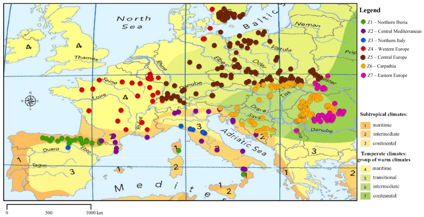
Our analysis covers 356 European beech stands distributed across seven climatic zones in the warm-subtropical and warm-temperate parts of Europe (Figure 1). Sampling locations were derived from the European Information System on Forest Genetic Resources (EUFGIS) genetic conservation units for Fagus sylvatica, which represent field-designated, beech-dominant forest stands. To ensure that sites represent clear beech stands, we retained only units in which Fagus sylvatica was reported as the dominant or main canopy species and in which the necessary metadata (coordinates and stand descriptors) were available in the EUFGIS database; units with ambiguous species dominance or incomplete information were excluded. The sites span the main west–east gradient of the species’ range, from the Atlantic-influenced Iberian Peninsula and France through Central Europe to the Carpathian and Black Sea regions, and cover a broad north–south gradient from the northern Alps and Baltic hinterland to southern Italy and the Balkans. According to the European Environment Agency’s main climate regions of Europe, climatic stratification follows a regional classification that distinguishes three subtropical climate types and four warm-temperate climate types. Sampling is densest in the central and eastern warm-temperate zones, where beech forms extensive, continuous forests, whereas fewer sites occur in the Iberian subtropical zones and the south-eastern continental zone. Because the EUFGIS network does not uniformly cover the entire distribution of F. sylvatica, our site set is not spatially exhaustive and may reflect sampling biases. For example, some areas are under-represented (e.g., southern United Kingdom, northern Germany, Austria, and parts of the Balkans), depending on data availability and designation of conservation units. Within each climatic zone, the elevations of beech locations were also considered, providing a consistent framework for comparing climate–phenology relationships across both macroclimatic regions and altitudinal gradients.

2.2. Data

The datasets used in this study fall into four main groups: (i) topography, (ii) climate and (iii) satellite-derived land-surface phenology, and (iv) high-resolution land cover for forest-purity quality control. All datasets were accessed and processed in Google Earth Engine (GEE).

Topographic information was derived from the Advanced Land Observing Satellite (ALOS) ALOS World 3D–30 m (AW3D30) Version 4.1 Digital Surface Model (DSM), produced by the Japan Aerospace Exploration Agency (JAXA) from Panchromatic Remote-sensing Instrument for Stereo Mapping (PRISM) imagery onboard the ALOS satellite. The product provides global coverage at approximately ±82° latitude with a 30 m spatial resolution and is openly available for research and educational use. The DSM was used solely to obtain elevation values at each of the 356 beech locations. Although EUFGIS/EUFORGEN provides elevation, we re-derived elevation from a DEM to ensure a spatially consistent and reproducible value for all sites (common reference, units, and coordinate handling) and to support uniform stratification.

Climatic variables were obtained from the ERA5-Land Daily Aggregated dataset produced by the European Centre for Medium-Range Weather Forecasts (ECMWF) under the Copernicus Climate Change Service (C3S). ERA5-Land combines observations with numerical weather prediction models to provide a spatially and temporally consistent reconstruction of past climate conditions. The dataset has a spatial resolution of ~0.1° (~11 km), a daily time step, and spans 1950 to the present, with an average 3-month latency. For each beech location, we extracted time series data of mean annual temperature and mean annual precipitation from ERA5-Land. These variables were used to characterize the climatic environment of each site and to analyze temporal trends and variability in climate across the seven climatic zones. Land-surface phenology metrics were derived from the MODIS MCD12Q2 Version 6.1 Land Cover Dynamics product, which provides annual phenological parameters at 500 m spatial resolution from 2001 onwards. The dataset is based on Two-Band Enhanced Vegetation Index (EVI2) time series from the combined Terra and Aqua MODIS sensors and includes, for each pixel, the timing of key phenophases, such as the start of greening, the date of maximum vegetation development, the end of season, and the growing-season length.

Within this study, MCD12Q2 was used to derive annual land-surface phenology metrics, including green-up (SOS), peak of season, and senescence (EOS). These metrics represent transition dates derived from changes in the satellite-observed EVI2 trajectory. Thus, they were interpreted as canopy or land-surface greenness transitions rather than as direct observations of individual-tree budburst, leaf discoloration, or leaf fall. The data were collected for 356 beech locations over the analysis period (2001–2024) and obtained from the EUFGIS database. Because MCD12Q2 is a 500 m, canopy-integrated product, we minimized mixed-pixel (understory/regeneration) effects by analyzing only beech-dominant EUFGIS stands and applying a WorldCover 10 m forest-homogeneity screen within 750 m of each site. These metrics were then related to ERA5-Land climate variables to quantify spatial and temporal patterns in beech phenology across climatic zones and elevation gradients and to assess their sensitivity to temperature and precipitation. Specifically, the day of year (DOY) of the SOS, peak of seasons, and EOS were used for the analysis.

ERA5-Land (~11 km) and MODIS phenology (500 m) differ substantially in spatial resolution. Therefore, we did not attempt pixel-to-pixel alignment. Instead, we used a site-based sampling approach: for each beech point, phenology was obtained from the MODIS 500 m pixel that contained the point, while climate variables were sampled from ERA5-Land at the same location. This assigns each site a consistent regional-scale climate forcing time series while retaining the finer-resolution phenological response at the canopy/land-surface scale.

Data Cleaning

To ensure the reliability of the climate and phenology analysis, we applied a series of filters to remove biologically and climatologically unrealistic outliers from the dataset. Because MODIS phenology is provided at 500 m resolution and individual pixels may contain mixed land cover (forest and non-forest), we applied a forest-homogeneity (purity) filter using European Space Agency (ESA) WorldCover (10 m) to reduce mixed-pixel effects at the site locations. For the climate variables, we retained only annual mean temperatures between −5 °C and 25 °C and annual total precipitation between 0 and 2500 mm, as values outside these ranges are implausible for the study regions. For phenology indicators expressed in DOY, we restricted the range to 50–330, thereby excluding invalid values such as 1 and values greater than 330 that could not represent realistic growing-season events.

For each EUFORGEN site, we calculated the percentage of tree-cover pixels from ESA WorldCover (10 m) within circular neighborhoods centered on the site (r = 750 m). We then retained only sites exceeding a minimum forest-cover threshold. To assess the sensitivity of the forest-homogeneity screening to neighborhood size, we tested a fixed minimum tree-cover threshold of 75% using radius of 500, 750, and 1000 m. These configurations retained 279, 275, and 271 sites, respectively. The 750 m radius was selected for the main analysis as an intermediate spatial neighborhood that reduced mixed land-cover influence while retaining broad site coverage. The main analysis uses a threshold of ≥75% tree cover within a 750 m radius, chosen to balance sample size and homogeneity.

The final dataset contained 6483 site–year records from 274 sites spanning 2001–2024 (see Supplementary Materials S1). After filtering, we generated two datasets: (i) a point-level dataset containing all valid observations per site and year, and (ii) an aggregated dataset summarizing yearly means per zone. This cleaning procedure minimized the influence of sensor errors and misclassified records (including mixed land-cover pixels in MODIS phenology) on subsequent trend and correlation analyses. After outlier cleaning, the dataset was retained in its point-level structure for the main analysis. The final dataset contained repeated annual observations for each site from 2001 to 2024, allowing long-term trend analysis (Figure 2). Elevation was included in the models as a continuous variable, whereas climatic zone was treated as a categorical factor representing regional ecological differences. Interactions involving year, elevation, and zone were included where relevant to evaluate spatial variation in temporal trends and climate sensitivities.

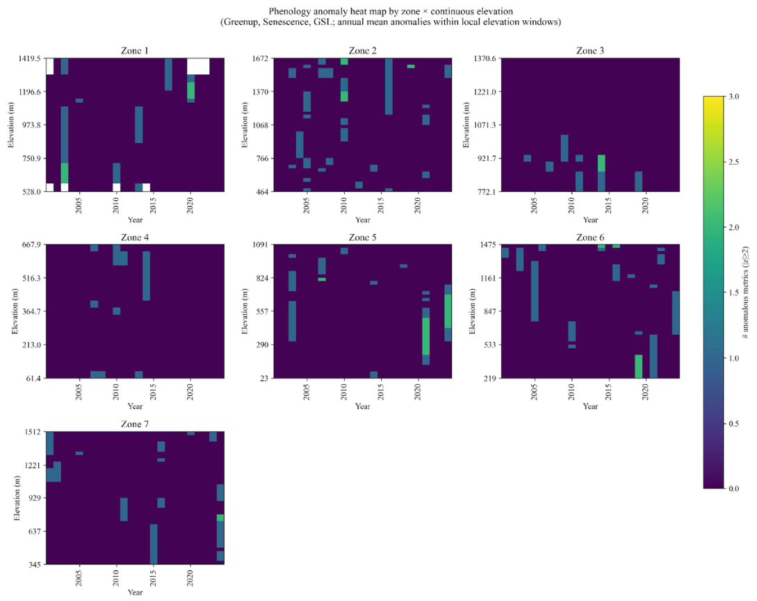
As an additional quality-control step, we quantified interannual phenological anomalies at the climatic zone level. For each group, we computed z-scores of annual green-up, peak of season, senescence, and GSL relative to the long-term mean and standard deviation. Years with |z| > 2 for any variable were flagged as anomalous. This procedure identified 40 anomalous zone–elevation–year combinations (≈10% of all 384 zone–elevation–year combinations) and 61 metric-level anomalies across Green-up, Peak, Senescence, and GSL.

2.3. Methods

2.3.1. Climate Trends

To assess climatic changes at the study sites, we analyzed annual mean temperature (°C) and total annual precipitation (mm/year) from 2001 to 2024. After data cleaning, each site was assigned to a climatic zone, while the elevation was retained as a continuous variable in the analysis. For each site–year observation, annual mean temperature and total annual precipitation values were retained for the analysis. These data were then used to estimate long-term trends by fitting mixed-effects models of climate variables against year. The slope of each regression was expressed both per year and per decade (e.g., °C/decade or mm/decade), allowing direct comparison of the rate of warming and changes in precipitation among zones and the elevation gradient. These trend estimates were interpreted to address two key questions: (i) which zones are warming fastest, and (ii) which exhibit drying or wetting trends in precipitation.

2.3.2. Phenology Trends

To quantify long-term shifts in phenological timing, we analyzed three key phenology metrics expressed as DOY: the onset of green-up, the peak of season, and the senescence date. After removing outliers, we fitted trend models for the 2001–2024 period. Phenological timing was modeled as a function of centered year, elevation, climatic zone, and their interactions, while accounting for repeated observations at the site level. The slope of each temporal trend represents the rate of change in phenology timing, expressed in days per year and rescaled to days per decade for interpretation. Negative slopes indicate that a phenological event is occurring earlier in the calendar year, while positive slopes indicate later timing. By comparing slopes across zones and the elevation gradient, we assessed spatial differences in the magnitude and direction of phenological responses to climate change.

In addition to the timing of individual phenophases, we calculated “spring duration” as the difference between peak and green-up dates (SpringDuration = Peak–Green-up) and estimated its temporal trend using the same trend analysis framework. This duration quantifies the time required for the canopy to transition from initial leaf expansion to peak biomass accumulation, thereby providing a simple proxy for the internal pace of spring development. We also tested whether elevation modified phenological trends differently among climatic zones using year × elevation × zone interactions. Temporal robustness was evaluated using GEE models with an AR (1) within-site correlation structure, and estimates were compared with the primary mixed-effects models. Residual spatial autocorrelation was assessed using Moran’s I based on site-level mean residuals and an eight-nearest-neighbor weights matrix. Because spatial dependence remained for some variables, we additionally used 1° × 1° spatial cells to obtain clustered standard errors and to test whether uneven sampling or dense site clusters influenced the zone-specific trends.

2.3.3. Phenoclimatic Sensitivity and Driver Attribution

To characterize the duration of the active canopy period, we calculated GSL as the difference between the DOY of senescence and the DOY of green-up. This metric represents the satellite-derived duration between green-up and senescence transitions.

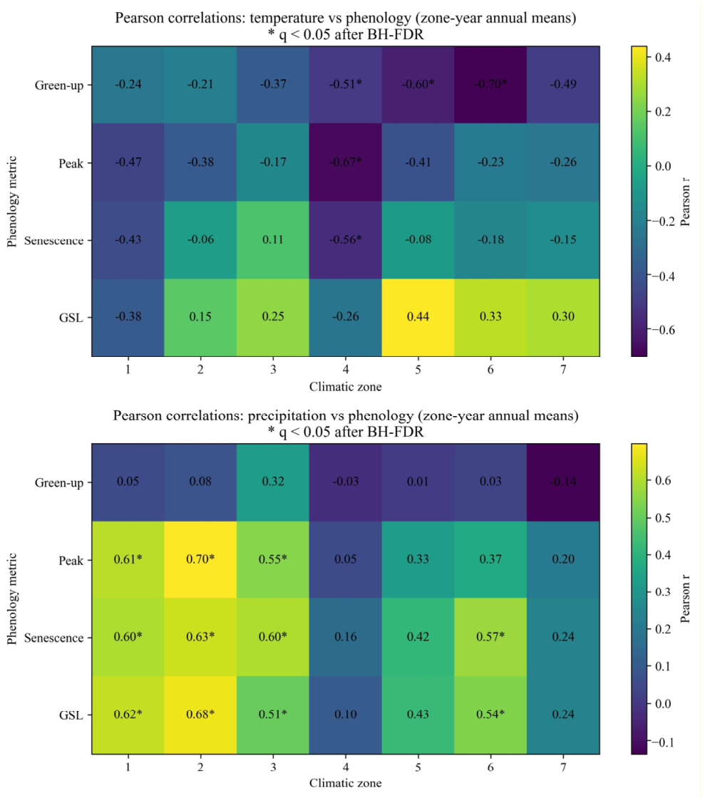
To describe bivariate associations between interannual climate variability and phenology timing, we computed Pearson correlations between annual climate variables (mean annual temperature–ta and total annual precipitation–Pcp) and phenology metrics (green-up, peak, senescence, and GSL). Correlations were computed on annual means within each climate zone, using the available annual observations within each zone.

Annual mean temperature and total annual precipitation were selected as broad-scale climatic descriptors applicable consistently across all sites and years. These variables were not intended to represent the full seasonal water balance or direct physiological drought stress. Accordingly, precipitation effects are interpreted as associations with regional moisture availability rather than as direct measures of growing-season drought intensity.

Because many climate–phenology pairs are evaluated, we addressed multiple testing by applying a Benjamini–Hochberg false discovery rate (FDR) correction across all correlation tests and report q-values.

To evaluate climatic associations with GSL while accounting for repeated measurements at the same sites, we fitted linear mixed-effects models on the site–year dataset:

$$GSLi,t=\beta 0+ \beta 1tai,t+\beta 2Pcp100i,t+\beta 3elevc,i+\gamma zone\left(i\right)+\delta zone\left(i\right)tai,t+\theta zoneiPcp100i,t+ui+\epsilon it$$

(1)

where $\beta 0$ is the overall intercept, corresponding to the expected GSL in the reference climatic zone when all continuous predictors are at their reference values; $\beta 1tai,t$: main effect of annual mean temperature; $\beta 2Pcp100i,t$: main effect of total annual precipitation on GSL; $\beta 3elevc,i$: main effect of elevation, included as a continuous covariate $\gamma zone\left(i\right)$: fixed effect of climatic zone; $\delta zone\left(i\right)tai,t$: zone-specific modification of the temperature effect; $\theta zoneiPcp100i,t$: zone-specific modification of the precipitation effect; $ui$: random intercept for site i; $\epsilon it$: residual error for site $i$ in year $t$.

To quantify the climatic drivers of growing-season length (GSL), we fitted a linear mixed-effects model with annual mean temperature, total annual precipitation, and continuous elevation as fixed effects. Climatic zone was included as a categorical factor, and interactions of zone with temperature and precipitation were added to allow climate sensitivities to vary among zones. Elevation was centered around its mean and scaled per 100 m. Site identity was included as a random intercept to account for repeated measurements from the same sites.

We fitted a mixed-effects model across the full site–year dataset, with elevation as a continuous predictor and climatic zone as a categorical factor, together with temperature, zone and precipitation, and zone interaction terms, to evaluate whether the climatic controls on GSL differed among zones. We also tested temperature × elevation × zone and precipitation × elevation × zone interactions for GSL.

2.3.4. Interannual Variability

To compare multivariate phenoclimatic profiles across climate zones, we developed a clustering framework integrating phenological trends, interannual variability, and climate–phenology sensitivities.

The analysis was performed on the climatic zones, and for each zone, we compiled a feature vector composed of eight metrics to quantify their unique phenoclimatic profile:

• Trends (days/decade): Green-up DOY, Senescence DOY, and GSL trend.
• Sensitivities (slopes): Green-up–Temperature slope (days/°C) and Senescence–Precipitation slope (days/mm).
• Drivers (correlation): GSL–Temperature (ρ) and GSL–Precipitation (ρ) Spearman correlation coefficients.
• Variability: Standard Deviation (SD) of Green-up timing.

All metrics were computed at the zone level from annual means (2001–2024) aggregated from site–year observations. Because the variables possessed different units and scales, all eight metrics (

Table 1. Variables used in this study.

Variable	Description	Unit	Source/Calculation
Green-up (SOS)	Start of season timing	DOY	MODIS MCD12Q2 phenology
Peak	Peak canopy greenness timing	DOY	MODIS MCD12Q2
Senescence (EOS)	End of season timing	DOY	MODIS MCD12Q2
GSL	Growing-season length	days	EOS−SOS
SpringDuration	Duration of spring canopy development	days	Peak−Green-up
Mean annual temperature	Annual thermal conditions	°C	ERA5-Land annual mean
Annual precipitation	Total annual precipitation	mm yr−¹	ERA5-Land annual sum
Elevation	Site elevation	m a.s.l.	ALOS AW3D30 DEM
Temperature trend	Long-term warming rate	°C decade−¹	Slope on year
Phenology trend	Long-term phenological change	days decade⁻¹	Slope on year
Composite phenoclimatic departure index	Composite metric	dimensionless	root-mean-square (RMS) of z-scores

) were converted to z-scores (standardization). This step ensures that metrics with naturally larger numerical magnitudes, such as trends or sensitivity slopes, do not disproportionately influence clustering results.

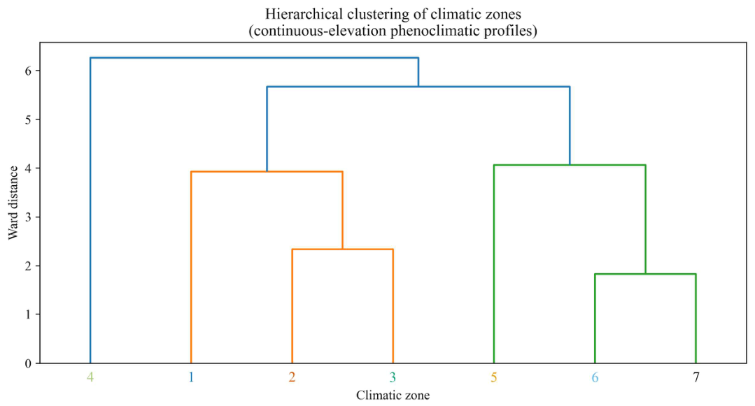
Euclidean distances were calculated from the standardized features, followed by hierarchical agglomerative clustering using Ward’s linkage. Cluster structure was evaluated by inspecting the dendrogram and by comparing silhouette scores across candidate numbers of clusters (k) values. We report a k = 2 solution for interpretability and provide a silhouette curve to document cluster validity.

Clusters were interpreted descriptively as regional phenoclimatic response profiles. Cluster interpretation was based on the relative configuration of phenological trends, climate sensitivities, and variability. Cluster labels were descriptive and were not treated as indicators of ecological risk, resilience, or demographic vulnerability.

In parallel, we derived a composite phenoclimatic departure index to summarize the overall magnitude of phenoclimatic change for each zone. This index combined six metrics: trends in annual mean temperature and precipitation (°C and mm per decade), trends in Green-up, Senescence, and GSL (days per decade), and the SD of Green-up timing. Each metric was first standardized to a z-score across all zones. The composite phenoclimatic departure index (CPDI) for a given stratum was then defined as the root-mean-square (RMS) of these six z-scores, as per Equation (2):

$$CPDI=\sqrt{{\displaystyle \frac{{z\left(T_z\right)}^2+{z\left(P_z\right)}^2+{z\left(G_z\right)}^2{z\left(S_z\right)}^2{+z\left(L_z\right)}^2+{z\left(V_z\right)}^2}{6}}}$$

(2)

where $z\left(T_z\right), z\left(P_z\right), z\left(G_z\right), z\left(S_z\right), z\left(L_z\right)$ and $z\left(V_z\right)$ are the standardized values of temperature trend, precipitation trend, green-up trend, senescence trend, GSL trend, and Green-up SD, respectively; higher values of this index indicate zones that deviate more strongly from the multi-stratum mean in terms of combined climatic trends, phenological shifts, and interannual variability.

CPDI is a relative, dimensionless measure of the magnitude of multivariate phenoclimatic departure from the cross-zone mean. Because it is direction-independent and equally weights all six standardized components, it was used only to compare departure among zones and not to classify ecological vulnerability, resilience, suitability, or risk. Equal weighting was retained because no independent empirical or theoretical basis was available for assigning different ecological importance to the six components.

To evaluate the robustness of this assumption, we additionally calculated a weighted CPDI under a series of sensitivity scenarios:

$${\mathrm{C}\mathrm{P}\mathrm{D}\mathrm{I}}_{\mathrm{z}}^{\left(\mathrm{s}\right)}=\sqrt{{\displaystyle \sum _{\mathrm{j}=1}^6}{\mathrm{w}}_{\mathrm{j}}^{\left(\mathrm{s}\right)}{\mathrm{Z}}_{\mathrm{z},\mathrm{j}}^2},{\displaystyle \sum _{\mathrm{j}=1}^6}{\mathrm{w}}_{\mathrm{j}}^{\left(\mathrm{s}\right)}=1$$

(3)

where ${\mathrm{w}}_{\mathrm{j}}^{\left(\mathrm{s}\right)}$ denotes the weight assigned to component j under sensitivity scenario s, and Z_z,j denotes the standardized value of component j for climatic zone z. For each component, its baseline weight of (1/6) was increased or decreased by 25%, while the weights of the remaining components were kept equal and renormalized to sum to one. We also performed a leave-one-component-out analysis, in which one component was assigned a weight of zero, and the remaining five components were weighted equally. Zone rankings from each scenario were compared with the equal-weight CPDI baseline using Spearman rank correlation.

3. Results

3.1. Climate Trends

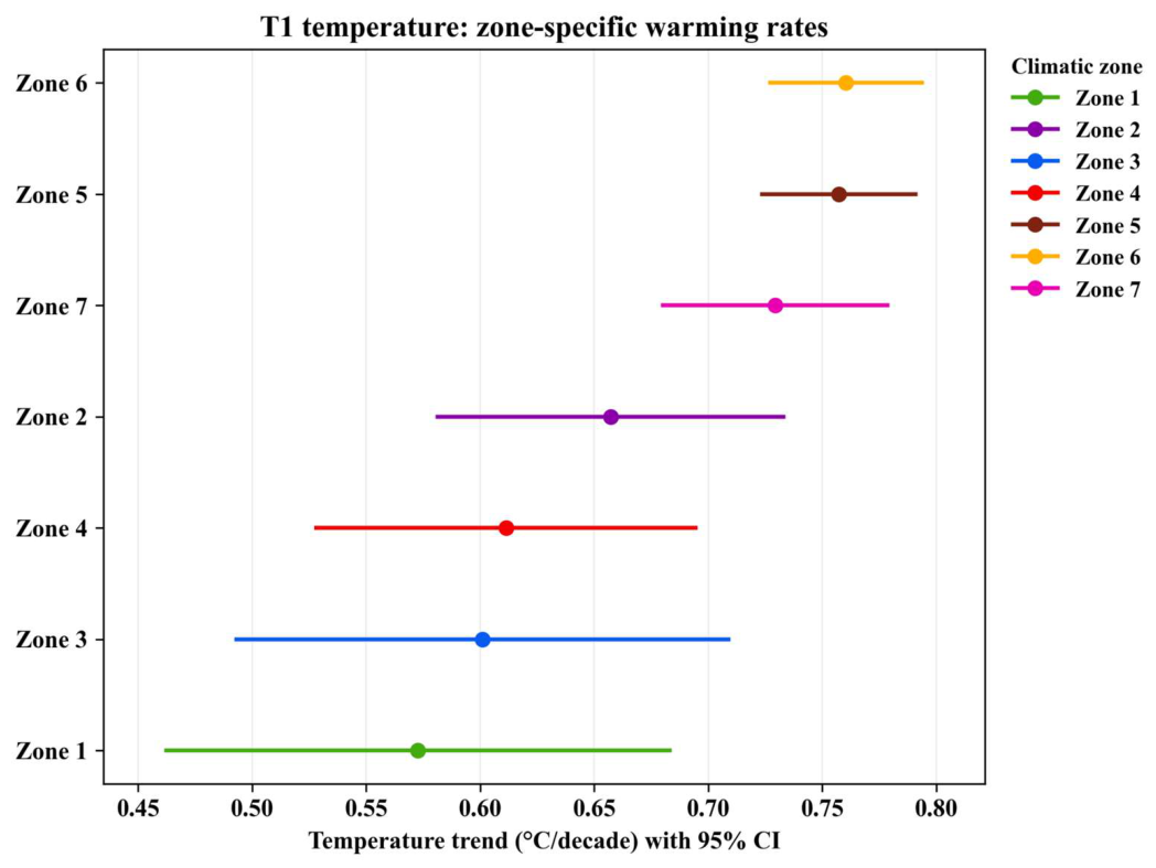
The analysis of climate trends shows that temperatures increased across all climatic zones during 2001–2024 (Figure 3;

Table 2. Zone-specific trends in annual mean temperature and total annual precipitation during 2001–2024, estimated from mixed-effects models. Trends are reported per decade with 95% confidence intervals.

Climatic zone	Temperature Trend (°C/Decade)	95% CI	p-Value	Precipitation Trend (mm/Decade)	95% CI	p-Value
Zone 1	0.57	0.46 to 0.68	<0.0001	58.05	30.41 to 85.70	<0.0001
Zone 2	0.66	0.58 to 0.73	<0.0001	27.54	8.45 to 46.63	0.0047
Zone 3	0.60	0.49 to 0.71	<0.0001	43.56	16.53 to 70.59	0.0016
Zone 4	0.61	0.53 to 0.69	<0.0001	40.40	19.53 to 61.27	<0.0001
Zone 5	0.76	0.72 to 0.79	<0.0001	2.73	−5.84 to 11.30	0.5328
Zone 6	0.76	0.73 to 0.79	<0.0001	−35.36	−43.86 to −26.87	<0.0001
Zone 7	0.73	0.68 to 0.78	<0.0001	−49.57	−62.03 to −37.10	<0.0001

). Estimated warming rates ranged from +0.57 °C/decade in Zone 1 (Northern Iberia) to +0.76 °C/decade in Zone 6 (Carpathia), with similarly strong warming also observed in Zone 5 (Central Europe) (+0.76 °C/decade) and Zone 7 (Eastern Europe) (+0.73 °C/decade). Intermediate warming rates were found in Zone 2 (Central Mediterranean) (+0.66 °C/decade), Zone 4 (Western Europe) (+0.61 °C/decade), and Zone 3 (Northern Italy) (+0.60 °C/decade). All temperature trends were statistically significant (p < 0.0001 for all zones).

For visual clarity in the accompanying time series figures, a 5-year running mean on the annual data are shown in the Supplementary Material (Figure S1). Supplementary Figuresshow the distribution of site-level slopes within each zone, indicating that although warming was consistent in direction, its magnitude still varied among sites within the same climatic zone (Figure S1).

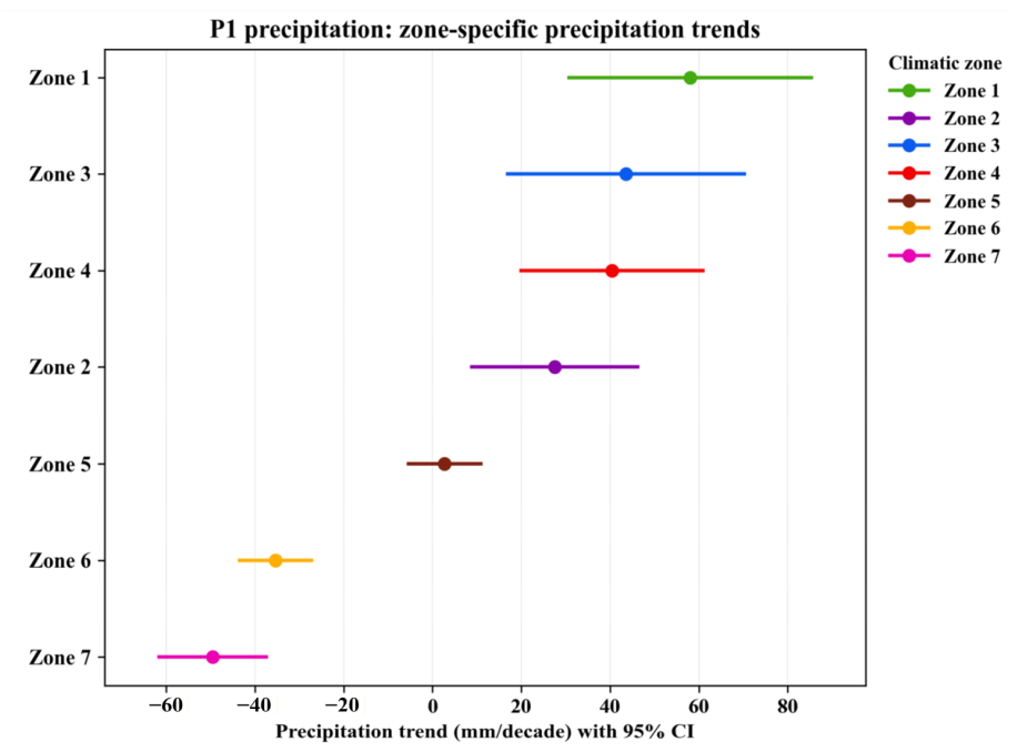
Precipitation trends were more heterogeneous, showcasing areas of both drying and wetting (Figure 4; Table 2). Significant wetting trends were detected in Zone 1-Northern Iberia (+58.1 mm/decade), Zone 3-Northern Italy (+43.6 mm/decade), Zone 4-Western Europe (+40.4 mm/decade), and Zone 2-Central Mediterranean (+27.5 mm/decade). In contrast, significant drying trends were observed in Zone 6 (−35.4 mm/decade) and Zone 7-Eastern Europe (−49.6 mm/decade). Zone 5-Central Europe showed only a weak and non-significant precipitation trend (+2.7 mm/decade, p = 0.5328). Thus, unlike temperature, precipitation did not show a uniform spatial pattern of change.

Descriptive annual precipitation series with linear trends and 5-year running means are provided in the Supplementary Material (Figure S2). These plots reveal considerably greater year-to-year variability in precipitation than in temperature. Site-level precipitation slopes also showed broader within-zone spread, especially in zones with positive wetting trends and in Zone 6-Carpathia, where drying dominated at the zone level, but substantial local variability remained (Figures S3 and S4).

3.2. Phenology Trends

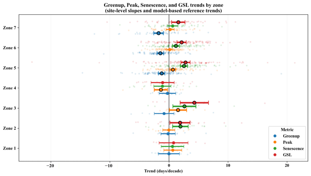
Long-term phenological trends varied across climatic zones, with the clearest signals observed in green-up advancement, delayed senescence, and increasing GSL. Peak timing showed more mixed responses (Figure 5; Table S1). The final analyses were conducted at the site–year level with elevation treated as a continuous predictor. Trends are presented here as zone-specific average marginal trends across the observed elevation range.

Green-up showed significant (p < 0.0001) advancement in the continental climate zones: Zone 5-Central Europe (−1.23 days/decade), Zone 6-Carpathia (−1.46 days/decade), and Zone 7-Eastern Europe (−1.74 days/decade), while the other zones showed weak or non-significant results (Table S1). Thus, earlier spring onset was not uniform across all zones but was mainly concentrated in the eastern and central parts of Europe.

Peak timing showed a more heterogeneous pattern. Significant delays were detected in Zone 3-Northern Italy (+1.54 days/decade) and Zone 5-Central Europe (+0.66 days/decade), while Zone 4-Western Europe showed a significant advance (−1.36 days/decade) (Table S1; Figure S5). Senescence trends were more coherent than peak trends and generally indicated delayed autumn timing in several zones. Significant delays were observed in Zone 2-Central Mediterranean (+1.95 days/decade), Zone 3-Northern Italy (+2.62 days/decade), Zone 5-Central Europe (+2.54 days/decade), and Zone 6-Carpathia (+1.18 days/decade), whereas the other zones did not show significant changes (Figures S6 and S7; Table S1).

Among all phenological metrics, GSL displayed the strongest and most spatially structured response (Figure S8; Table S1). In the primary mixed-effects models, significant GSL increases were found in Zone 2-Central Mediterranean (+1.88 days/decade), Zone 3-Northern Italy (+4.30 days/decade), Zone 5 (+2.81 days/decade), Zone 6-Carpathia (+2.14 days/decade), and Zone 7-Eastern Europe (+1.58 days/decade).

The phenology results indicate that the dominant signal was not a continent-wide, uniform shift in a single phenophase, but rather a combination of earlier green-up and later senescence in selected climatic zones, resulting in significant lengthening of the growing season in several regions. Elevation modified green-up and senescence trends differently among zones (p = 0.0037 and p = 0.0137), but not peak timing or GSL trends (p = 0.286 and p = 0.232) (Table S2).

Spring Development Duration, used as an index of the internal pace of spring canopy development, showed limited evidence for systematic change. Only Zone 5-Central Europe exhibited a significant lengthening (+1.62 days/decade, p = 0.0002), and Zone 6 (+1.02 days/decade, p = 0.003), while other strata were not significant. We also tested quadratic time effects but found no consistent evidence of nonlinear trends; therefore, linear slopes were retained.

GEE models with an AR (1) within-site correlation structure produced results broadly consistent with the primary mixed-effects models. Most trend directions and significance classifications were unchanged, although Zone 2 GSL changed significance and peak timing was more model-sensitive (Figures S11 and S12). Residual spatial dependence was weak for green-up and GSL and stronger for peak timing and senescence. Spatially clustered analyses retained the main trend directions, although several marginal estimates changed significance (Figure S13). Uncertainty was greater in sparsely represented zones.

3.3. Phenoclimatic Sensitivity and Driver Attribution

Here, climate sensitivity refers to the estimated change in a phenological metric per unit change in temperature or precipitation.

The sensitivity analysis confirms a widespread, yet heterogeneous, coupling between beech phenology and interannual climate variability. As expected, green-up timing tends to advance under warmer conditions, consistent with a strong association between spring timing and temperature. However, the strength and statistical robustness of this relationship vary across climatic zones. The strongest temperature-related responses were observed in Zones 5, 6, and 7, where earlier green-up was also evident in the trend analysis (Table S1). In contrast, other zones showed weaker or non-significant sensitivities, suggesting that unmeasured local conditions may contribute to the remaining variation.

Timing of senescence showed clearer links to water availability across multiple zones. Senescence exhibited positive precipitation sensitivities (later senescence in wetter years). This pattern also indicates that, in some regions, autumn timing showed stronger associations with precipitation than with temperature in some zones. To quantify climatic associations while accounting for repeated measurements at clustered sites, we fitted mixed-effects models on site–year data, using GSL as the response and annual temperature and precipitation as predictors, with random intercepts for site. At the overall model level, both thermal and hydrological variability contributed to GSL variability. However, their effects differed among climatic zones (Figure S8). The estimated random-intercept variance indicates substantial site-to-site differences in mean GSL, supporting the need for a hierarchical framework. The results showed the strongest temperature effect on GSL in Zone 3-Northern Italy with +4.05 days per 1 °C (95% Cl: 1.80 to 6.31). Significant positive temperature effects were also noticed in Zone 5-Central Europe, +1.57, Zone 6-Carpathia, +2.07, and Zone 7-Eastern Europe, +2.37 days per 1 °C. The strongest precipitation effect was noticed on Zone 5, +1.57 per 100 mm (95% Cl 1.46 to 2.35), followed by Zone 2-Central Mediterranean (+0.95), Zone 3-Northern Italy (+1.47), Zone 6-Carpathia (+1.49), and Zone 7-Eastern Europe (+1.53 days per 100 mm). Zone 1-Northern Iberia and Zone 4-Western Europe showed non-significant effects for both predictors (

Table 3. Zone-specific effects of annual mean temperature and annual precipitation on GSL, estimated from mixed-effects models with elevation included as a continuous predictor and site as a random intercept.

Climatic Zone	Temperature Effect on GSL (Days Per 1 °C)	95% CI	Precipitation Effect on GSL (Days Per 100 mm	95% CI
Zone 1	−0.24	−2.20 to 1.72	0.37	−0.66 to 1.40
Zone 2	0.81	0.03 to 1.58	0.95	0.45 to 1.45
Zone 3	4.05	1.80 to 6.31	1.47	0.64 to 2.31
Zone 4	−1.15	−2.66 to 0.37	0.72	−0.34 to 1.79
Zone 5	1.57	0.93 to 2.20	1.91	1.46 to 2.35
Zone 6	2.07	1.48 to 2.66	1.49	1.16 to 1.82
Zone 7	2.37	1.30 to 3.44	1.53	0.84 to 2.22

). Elevation did not significantly modify temperature sensitivity among zones (p = 0.579), but it significantly modified precipitation sensitivity (p = 0.0041).

3.4. Growing-Season Dynamics

Growing-season length integrates the timing of spring green-up and autumn senescence but does not directly measure productivity. Under the thr75–r750 filtering, mean site–year GSL values were on the order of ~117 days (site-level variability is substantial; see mixed-model variance components in Supplementary Materials S1). Long-term trends (2001–2024) remained spatially heterogeneous (Figure 6). Statistically significant GSL lengthening was detected in Zone 3 (+4.30 days/decade, p = 0.0004), Zone 5 (+2.81 days/decade, p < 0.0001), Zone 6 (+2.14 days/decade, p < 0.0001), Zone 2 (+1.88 days/decade, p = 0.0305), and Zone 7 (+1.58 days/decade, p = 0.0061). In contrast, Zones 1 and 4 showed non-significant trends. These results emphasize that the net effect of earlier spring transitions and later autumn transitions is strongly zone-dependent, consistent with the mixed-model driver classification above. The primary mixed-effects model indicated a positive trend in Zone 2, but its significance was not retained in the AR (1) sensitivity analysis.

3.5. Interannual Variability

We quantified interannual variability as the SD of green-up, peak timing, senescence, and GSL across climatic zones using the final continuous-elevation framework. Green-up variability was generally moderate across zones, with the lowest values observed in Zone 3-Northern Italy and the highest in Zone 5-Central Europe, indicating that year-to-year spring timing was not equally stable across the study domain. Peak timing showed comparable dispersion, while senescence variability was of similar magnitude in several zones. Interannual variability in GSL also varied among zones, reflecting the combined year-to-year variability of both spring and autumn transitions. This indicates that the seasonal response of beech is not temporally uniform among climatic zones.

Extreme phenological anomalies (|z| > 2) relative to the local 2001–2024 mean and SD occurred across multiple zones and elevation windows. In the final filtered dataset, 862 metric-level anomalies were detected, corresponding to 568 site–year observations in which at least one phenology metric was anomalous. Anomaly years were not confined to a single period, but instead appeared intermittently across the record, with the largest concentrations observed in 2021 (141 anomalous observations), 2024 (135), 2018 (88), and 2010 (57) (Figure 7). The anomaly heat map further shows that these events were not uniformly distributed across space, but were concentrated in specific year–elevation windows within zones, especially in Zones 5-Central Europe, Zone 6-Carpathia, and Zone 7-Eastern Europe. These results show that the time series includes both gradual directional trends and episodic anomalous years.

3.5.1. Clustering of Climatic Zones by Phenology and Climate

To synthesize multi-dimensional phenoclimatic information, we applied Ward’s hierarchical clustering to the climatic zones using standardized phenological and climatic variables (Figure 8; see Supplementary Materials S1). The dendrogram indicated a separation among climatic zones based on their combined phenological trends, climate–phenology sensitivities, and interannual variability. Candidate clustering solutions were evaluated using silhouette scores, which were highest for k = 2 (0.253), with progressively lower support for k = 3 (0.223), k = 4 (0.206), and k = 5 (0.190) (Figure 8). Based on the selected k = 2 solution, two phenoclimatic clusters were identified and ecologically interpreted (

Table 4. Ecological interpretation of the clusters.

Cluster	Climatic Zones	Ecological Interpretation
1	Zone 4	Distinct/weak-direction system with comparatively low senescence and GSL trends, weak climate–phenology sensitivities, and an atypical phenoclimatic profile;
2	Zone 1–3; Zone 5–7	Broad climate-responsive regime, with varying degrees of phenological change, GSL lengthening and climate coupling across zones

).

Cluster 1 is represented by Zone 4-Western Europe and reflects a distinct phenoclimatic profile characterized by relatively weak senescence and GSL trends, low climate– phenology sensitivities, and an atypical position relative to the rest of the study domain.

Cluster 2 represents the main climate-responsive regime and includes the remaining zones. The separation indicates that climatic zones differ in the combination of phenological trends and climate associations.

3.5.2. Composite Phenoclimatic Departure Index

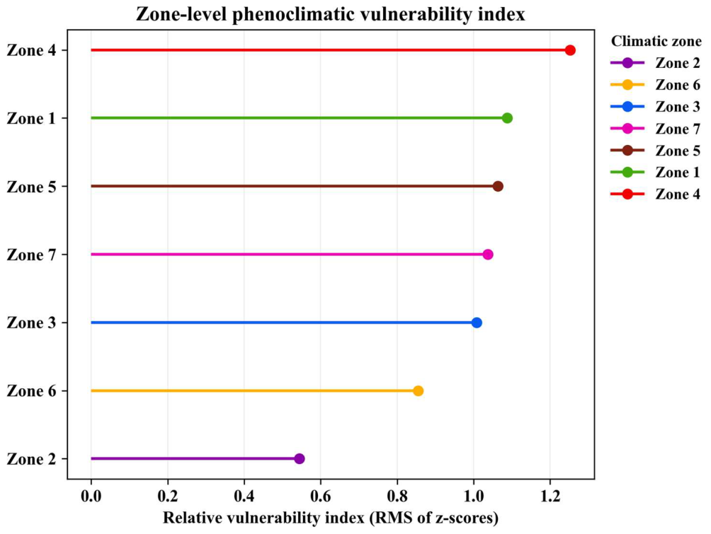
As a separate exploratory synthesis, we calculated a composite phenoclimatic departure index based on the root-mean-square of six standardized components: annual temperature trend, annual precipitation trend, green-up trend, senescence trend, GSL trend, and green-up interannual variability. Higher values indicate a larger combined departure from the multi-zone mean across climatic forcing, phenological shifts, and variability (Figure 9). Because the index is direction-independent, it should not be interpreted as an absolute measure of ecological risk or as a substitute for the pathway-specific phenological responses described above.

The weight-sensitivity analysis indicated that the overall CPDI pattern was broadly robust to moderate changes in component weighting. Across the ±25% weight-perturbation and leave-one-component-out scenarios, Zone 4 generally remained at the high-departure end of the gradient, whereas Zone 2 consistently retained the lowest rank. Intermediate zones showed greater rank variability and partially overlapping CPDI ranges, indicating that their exact ordering was more sensitive to the weighting scheme (Figures S9 and S10).

At the zone level, the highest phenoclimatic departure score was observed in Zone 4-Western Europe (index = 1.25), followed by Zone 1-Northern Iberia (1.09), Zone 5-Central Europe (1.06), Zone 7-Eastern Europe (1.04), and Zone 3-Northern Italy (1.01). Lower departure values were found in Zone 6-Carpathia (0.85), whereas Zone 2-Central Mediterranean showed the lowest score (0.54). These results indicate that Zone 4-Western Europe departs most strongly from the overall multi-zone mean across combined climatic trends, phenological shifts, and green-up variability, while Zone 2-Central Mediterranean shows the smallest overall departure. The high CPDI of Zone 4 reflects a large multivariate departure from the cross-zone mean and does not imply greater ecological risk.

4. Discussion

4.1. Climate and Phenological Responses

The climate-trend results highlight the need for regionally tailored adaptive forest management strategies, particularly given the compounded risks of strong warming across all climatic zones and spatially contrasting wetting and drying trends.

Across 2001–2024, warming was statistically significant across all of the beech range, with the strongest trends observed in Zone 5, 6 and 7, in line with long-term European warming and associated phenological shifts reported in previous studies [28,31,66,67]. The spatial consistency of this warming signal supports the interpretation that thermal forcing is now a pervasive background driver of phenological change across European beech sites.

On the other hand, precipitation trends are spatially heterogeneous. While some regions show only weak changes, others show a marked drying or wetting trend, consistent with projections of increasing aridity and drought risk in Mediterranean and subtropical continental climates [68]. This pattern reinforces concerns about drought sensitivity at the southern and eastern margins of the European beech distribution. Together, these climatic gradients explain why phenological responses are strongly zone-dependent; some zones are dominated by warming alone, whereas others are shaped by the combined effects of warming and shifting moisture availability.

4.2. Spring and Autumn Phenology, and Anomalous Spring Development

Our phenological analysis confirms a heterogeneous phenological response across climatic zones. Green-up advanced significantly in Zones 5, 6 and 7, confirming the high thermal sensitivity of spring onset in deciduous forests [67]. In line with broader Northern Hemisphere findings, warmer springs are associated with earlier leaf-out (mean temperature–spring onset correlations around −0.3) [69]. Trends in Zones 1–4 were weak and non-significant, indicating that earlier spring onset is not uniform across the species range. MODIS-derived SOS and EOS represent canopy-scale EVI2 transitions rather than direct observations of individual-tree budburst or leaf fall. Accordingly, the observed trends indicate changes in land-surface phenology rather than exact shifts in individual-tree phenophases.

In contrast, senescence shifts are more spatially structured, with significant delays in Zones 2, 3, 5 and 6, which is consistent with previous reports of slightly later autumn phenology in Europe [67], but strongly modulated by summer moisture availability and drought events [69].

Peak timing showed a more mixed pattern than either Green-up or Senescence, with a significant delay in Zones 3 and 5 but an advance in Zone 4. This suggests that the rate of spring canopy development does not respond uniformly across climatic zones, even when Green-up itself advances.

Among the phenological metrics, GSL provided the clearest integrated signal. Significant lengthening of the growing season was detected in Zones 2, 3, 5, 6, and 7, with the strongest increase in Zone 3. This indicates that the most robust phenological response was not a uniform shift in a single phenophase, but rather the combined effect of earlier spring onset and/or later autumn timing, resulting in longer effective growing seasons in several climatic zones. The coexistence of significant GSL lengthening with heterogeneous Green-up, Peak, and Senescence responses also suggests that phenological change in beech is increasingly regime-dependent rather than uniform across Europe.

The combination of earlier green-up and longer GSL in Zones 5–7 is particularly notable because these regions overlap with areas that experienced severe impacts during the 2018–2020 hot drought sequence, including widespread early wilting, premature leaf shedding, and elevated forest disturbance [51,52]. Earlier bud break and leaf unfolding may increase transpiration demand and lengthen the period of canopy water use, potentially increasing exposure to summer soil moisture deficits and atmospheric drought stress. Thus, although warmer springs can promote earlier canopy development, these gains do not necessarily translate into improved seasonal performance under increasingly frequent hot drought conditions [48,49,50]. In contrast, the Mediterranean zones showed weaker advances in Green-up and a greater contribution of delayed Senescence to GSL extension. Together, these contrasting phenological pathways suggest that similar increases in GSL may correspond to very different hydrological and physiological consequences across the range of European beech.

4.3. Phenoclimatic Profiles, GSL Drivers

Site–year models showed that climate–GSL associations varied substantially among zones. Temperature remained an important covariate of spring timing and growing-season structure, while its associations varied with water availability and regional context. In some zones, GSL variability was more strongly associated with temperature, whereas in others, precipitation played a larger role, indicating that similar GSL changes may arise through different regional climatic pathways.

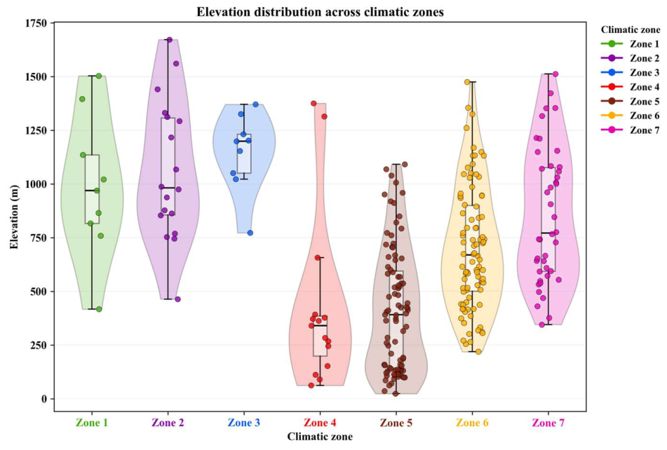
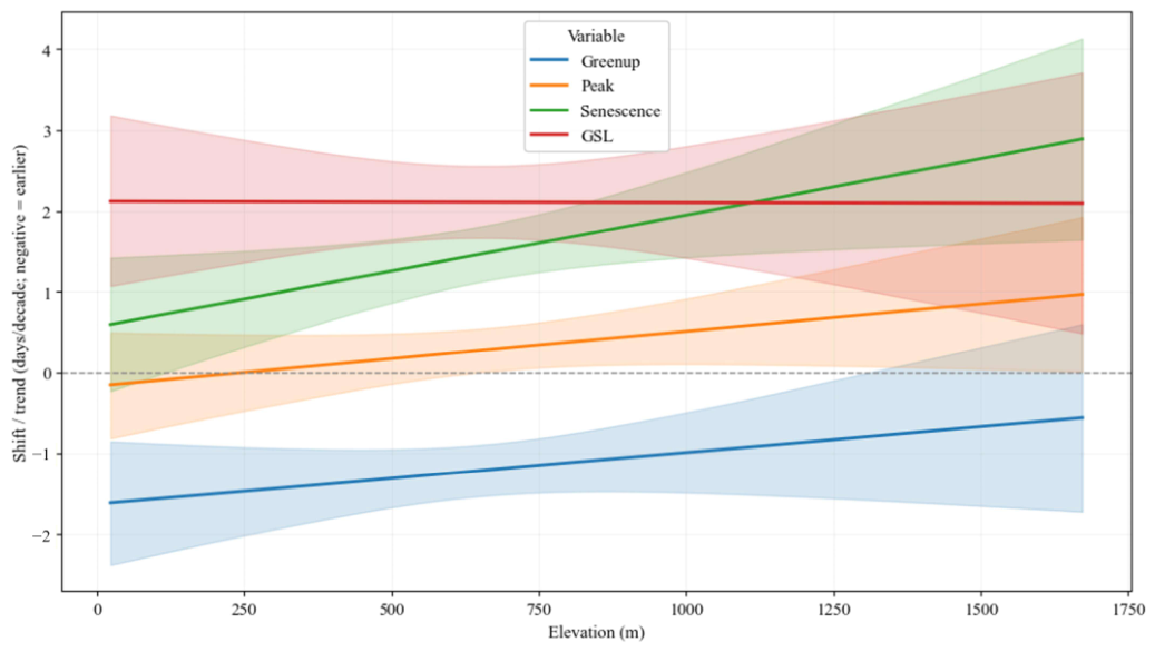
Zone-specific trends in green-up, senescence, and GSL further confirmed spatial heterogeneity. Elevation was retained as a continuous predictor (Figure 10). Elevation modified green-up and senescence trends differently among climatic zones, but not peak timing or GSL trends. Elevation also modified precipitation sensitivity among zones, whereas temperature sensitivity showed no significant elevation-dependent variation. GSL extension was robust in Zones 3, 5, 6, and 7, while the positive Zone 2 estimate was more model-sensitive. These findings indicate that growing-season extension depends on both thermal opportunity and regional water availability.

Following WorldCover-based homogeneity filtering, the zone-level clustering identified two descriptive phenoclimatic groups:

• Cluster 1: Zone 4. This zone shows a distinct phenoclimatic profile, with relatively weak senescence and GSL trends, weak climatic sensitivities, and the highest composite phenoclimatic departure score, indicating an atypical profile.
• Cluster 2: Zones 1, 2, 3, 5, 6, and 7. This is the dominant climate-responsive regime, showing greater phenological change and clearer climate coupling, although the magnitude and direction of individual responses differ among zones.

The clustering describes the configuration of zone-level phenoclimatic responses, whereas CPDI summarizes the magnitude of multivariate departure. Because both analyses share several input variables, they should not be treated as independent validation. The CPDI should therefore be interpreted as a relative screening index of multivariate phenoclimatic departure rather than as a ranking of ecological condition or risk.

The CPDI sensitivity analysis showed that Zone 4 remained at the high-departure end and Zone 2 at the low-departure end, while the ordering of intermediate zones varied.

From a management and genetic perspective, these phenoclimatic profiles may indicate contrasting regional exposure and response pathways. Thermally responsive montane stands may benefit from longer growing seasons but face increased frost and extreme-event risks [70,71,72]. Zones with stronger precipitation associations may be more exposed to moisture limitation, although this requires confirmation using seasonal drought indicators. These patterns should be validated before informing seed-source decisions.

4.4. Limitations and Future Directions

The remote-sensing framework applied here provides a consistent, pan-European view of beech phenology, but several limitations must be acknowledged. First, MODIS phenology at 500 m resolution inevitably includes mixed pixels in heterogeneous landscapes, and we cannot fully resolve pure beech stands from co-occurring broadleaves or conifers in all cases. In addition, MCD12Q2 phenological transition dates are derived from EVI2 trajectories and are not direct observations of budburst, leaf discoloration, or leaf fall. Differences between satellite-derived and ground-observed phenophases may arise from canopy integration, mixed vegetation signals, temporal compositing, and the definition of the EVI2 transition threshold. Therefore, phenoclimatic patterns and CPDI should be interpreted as indicators of relative changes in canopy-scale land-surface phenology, rather than as direct measures of physiological stress, ecological damage, or absolute vulnerability. The coarser spatial resolution of ERA5-Land may also smooth local climatic variability associated with topography, exposure, and other site-specific conditions. Therefore, the climate–phenology relationships identified here should be interpreted at the regional and climatic-zone scales rather than as local 500 m pixel-level responses. Future studies could assess the sensitivity of these relationships using higher-resolution climate datasets or multi-scale comparisons. Although alternative neighborhood sizes were evaluated, the sensitivity analysis did not include multiple tree-cover thresholds. The selected 75% criterion may exclude genuine but heterogeneous, fragmented, or mixed beech stands, and the final sample therefore emphasizes relatively homogeneous forest conditions. Second, climatic drivers are represented by annual mean temperature and precipitation, which only approximate the seasonal and water-balance metrics, e.g., VPD and the Standardized Precipitation Evapotranspiration Index (SPEI), that directly affect phenology. Annual precipitation cannot distinguish between growing-season and dormant-season moisture availability and does not capture atmospheric drought or climatic water balance. The omission of variables such as growing-season VPD and SPEI therefore limits the physiological interpretation of the observed precipitation–phenology relationships. Third, stand structure, age, management history, and soil properties are not explicitly included, even though they can modulate climate–phenology relationships. Finally, we assume linear trends and linear responses, whereas threshold behavior and non-linear dynamics may emerge under stronger or more prolonged climate forcing.

Residual spatial autocorrelation remained strongest for peak timing and senescence. Spatially clustered analyses retained the main trend directions, although some marginal estimates changed significance. Geographic gaps in the EUFGIS network remain a source of uncertainty.

Future work should integrate Sentinel-2, PhenoCam, UAV, tree-ring, crown-condition, regeneration, provenance, and genetic data to validate the phenoclimatic patterns identified here. Seasonally resolved drought indicators, including growing-season VPD and multimonth SPEI, are also needed to distinguish atmospheric and soil-moisture constraints and to evaluate potential future climate refugia or retreat zones.

5. Conclusions

This study shows that climate change is reshaping Fagus sylvatica phenology across Europe in a highly non-uniform way, structured by regional climate context and contrasting phenological pathways. By applying a strict land-cover homogeneity filter (WorldCover; ≥75% tree cover within r = 750 m), we reduced the influence of mixed MODIS pixels and derived a more conservative, beech-dominant signal.

Under this filtered analysis, the phenoclimatic typology is best described as a dominant climate-responsive regime contrasted with a distinct outlying zone, rather than a single high-elevation “accelerator” cluster spanning multiple regions. Zone 4-Western Europe emerges as a distinct phenoclimatic type with comparatively weak climatic sensitivities, whereas the rest of the zones form the main climate-responsive regime. This distinction reflects differences in the configuration of phenological trends, climate sensitivities, and variability, and should not be interpreted as a ranking of ecological vulnerability, resilience, or risk.

Our findings emphasize that an extended growing season does not necessarily indicate higher productivity or resilience. The phenoclimatic typology and CPDI describe contrasting regional response and departure patterns rather than ecological condition or risk. These patterns can guide further monitoring and independent ecological validation. Remote sensing provides an operational means to track phenological trends and anomalies and support adaptive management of European beech forests under ongoing climate change.

References

1. Kaplan, G.; Özbey, A.A. Identifying Environmental Constraints on Pinus brutia Regeneration Using Remote Sensing: Toward a Screening Framework for Sustainable Forest Management. Forests 2025, 16, 1816. [Google Scholar] [CrossRef]
2. Geßler, A.; Keitel, C.; Kreuzwieser, J.; Matyssek, R.; Seiler, W.; Rennenberg, H. Potential Risks for European Beech (Fagus sylvatica L.) in a Changing Climate. Trees 2006, 21, 1–11. [Google Scholar] [CrossRef]
3. Schuldt, B.; Buras, A.; Arend, M.; Vitasse, Y.; Beierkuhnlein, C.; Damm, A.; Gharun, M.; Grams, T.E.E.; Hauck, M.; Hajek, P.; et al. A First Assessment of the Impact of the Extreme 2018 Summer Drought on Central European Forests. Basic Appl. Ecol. 2020, 45, 86–103. [Google Scholar] [CrossRef]
4. Rukh, S.; Sanders, T.G.M.; Krüger, I.; Schad, T.; Bolte, A. Distinct Responses of European Beech (Fagus sylvatica L.) to Drought Intensity and Length—A Review of the Impacts of the 2003 and 2018–2019 Drought Events in Central Europe. Forests 2023, 14, 248. [Google Scholar] [CrossRef]
5. Kariyeva, J.; Van Leeuwen, W.J.D.; Woodhouse, C.A. Impacts of Climate Gradients on the Vegetation Phenology of Major Land Use Types in Central Asia (1981–2008). Front. Earth Sci. 2012, 6, 206–225. [Google Scholar] [CrossRef]
6. Lukasová, V.; Vido, J.; Škvareninová, J.; Bičárová, S.; Hlavatá, H.; Borsányi, P.; Škvarenina, J. Autumn Phenological Response of European Beech to Summer Drought and Heat. Water 2020, 12, 2610. [Google Scholar] [CrossRef]
7. Skvareninova, J.; Sitko, R.; Vido, J.; Snopková, Z.; Skvarenina, J. Phenological Response of European Beech (Fagus sylvatica L.) to Climate Change in the Western Carpathian Climatic-Geographical Zones. Front. Plant Sci. 2024, 15, 1242695. [Google Scholar] [CrossRef] [PubMed]
8. Bolte, A.; Czajkowski, T.; Kompa, T. The North-Eastern Distribution Range of European Beech a Review. Forestry 2007, 80, 413–429. [Google Scholar] [CrossRef]
9. Brunet, J.; Fritz, Ö.; Richnau, G. Biodiversity in European Beech Forests-a Review with Recommendations for Sustainable Forest Management. Ecol. Bull. 2010, 53, 77–94. [Google Scholar]
10. Magri, D.; Vendramin, G.G.; Comps, B.; Dupanloup, I.; Geburek, T.; Gömöry, D.; Latałowa, M.; Litt, T.; Paule, L.; Roure, J.M.; et al. A New Scenario for the Quaternary History of European Beech Populations: Palaeobotanical Evidence and Genetic Consequences. New Phytol. 2006, 171, 199–221. [Google Scholar] [CrossRef] [PubMed]
11. Magri, D. Patterns of Post-glacial Spread and the Extent of Glacial Refugia of European Beech (Fagus sylvatica). J. Biogeogr. 2008, 35, 450–463. [Google Scholar] [CrossRef]
12. Saltré, F.; Saint-Amant, R.; Gritti, E.S.; Brewer, S.; Gaucherel, C.; Davis, B.A.S.; Chuine, I. Climate or Migration: What Limited European Beech Post-glacial Colonization? Glob. Ecol. Biogeogr. 2013, 22, 1217–1227. [Google Scholar] [CrossRef]
13. Cai, Q.; Welk, E.; Ji, C.; Fang, W.; Sabatini, F.M.; Zhu, J.; Zhu, J.; Tang, Z.; Attorre, F.; Campos, J.A.; et al. The Relationship between Niche Breadth and Range Size of Beech (Fagus) Species Worldwide. J. Biogeogr. 2021, 48, 1240–1253. [Google Scholar] [CrossRef]
14. Pramreiter, M.; Grabner, M. The Utilization of European Beech Wood (Fagus sylvatica L.) in Europe. Forests 2023, 14, 1419. [Google Scholar] [CrossRef]
15. Besliu, E.; Curtu, A.L.; Apostol, E.N.; Budeanu, M. Using Adapted and Productive European Beech (Fagus sylvatica L.) Provenances as Future Solutions for Sustainable Forest Management in Romania. Land 2024, 13, 183. [Google Scholar] [CrossRef]
16. Fuchs, Z.; Vacek, Z.; Vacek, S.; Cukor, J.; Šimůnek, V.; Štefančík, I.; Brabec, P.; Králíček, I. European Beech (Fagus sylvatica L.): A Promising Candidate for Future Forest Ecosystems in Central Europe amid Climate Change. Cent. Eur. For. J. 2024, 70, 62–76. [Google Scholar] [CrossRef]
17. Liepiņš, K.; Bleive, A. The Potential of European Beech (Fagus sylvatica L.) in the Hemiboreal Baltic Region: A Review. Forests 2025, 16, 109. [Google Scholar] [CrossRef]
18. Budeanu, M.; Petritan, A.M.; Popescu, F.; Vasile, D.; Tudose, N.C. The Resistance of European Beech (Fagus sylvatica) From the Eastern Natural Limit of Species to Climate Change. Not. Bot. Horti Agrobot. Cluj-Napoca 2016, 44, 625–633. [Google Scholar] [CrossRef]
19. Leuschner, C.; Bat-Enerel, B. Effects of Heat, Elevated Vapor Pressure Deficits and Growing Season Length on Growth Trends of European Beech. Front. For. Glob. Change 2024, 7, 1489081. [Google Scholar] [CrossRef]
20. Leuschner, C. Drought Response of European Beech (Fagus sylvatica L.)—A Review. Perspect. Plant Ecol. Evol. Syst. 2020, 47, 125576. [Google Scholar] [CrossRef]
21. Gárate-Escamilla, H.; Hampe, A.; Vizcaíno-Palomar, N.; Robson, T.M.; Benito Garzón, M. Range-wide Variation in Local Adaptation and Phenotypic Plasticity of Fitness-related Traits in Fagus sylvatica and Their Implications under Climate Change. Glob. Ecol. Biogeogr. 2019, 28, 1336–1350. [Google Scholar] [CrossRef]
22. Pfenninger, M.; Reuss, F.; Kiebler, A.; Schönnenbeck, P.; Caliendo, C.; Gerber, S.; Cocchiararo, B.; Reuter, S.; Blüthgen, N.; Mody, K.; et al. Genomic Basis for Drought Resistance in European Beech Forests Threatened by Climate Change. eLife 2021, 10, e65532. [Google Scholar] [CrossRef] [PubMed]
23. Cavin, L.; Jump, A.S. Highest Drought Sensitivity and Lowest Resistance to Growth Suppression Are Found in the Range Core of the Tree Fagus sylvatica L. Not the Equatorial Range Edge. Glob. Change Biol. 2017, 23, 362–379. [Google Scholar] [CrossRef] [PubMed]
24. Arend, M.; Link, R.M.; Zahnd, C.; Hoch, G.; Schuldt, B.; Kahmen, A. Lack of Hydraulic Recovery as a Cause of Post-drought Foliage Reduction and Canopy Decline in European Beech. New Phytol. 2022, 234, 1195–1205. [Google Scholar] [CrossRef] [PubMed]
25. Frei, E.R.; Gossner, M.M.; Vitasse, Y.; Queloz, V.; Dubach, V.; Gessler, A.; Ginzler, C.; Hagedorn, F.; Meusburger, K.; Moor, M.; et al. European Beech Dieback after Premature Leaf Senescence during the 2018 Drought in Northern Switzerland. Plant Biol. 2022, 24, 1132–1145. [Google Scholar] [CrossRef] [PubMed]
26. Root, T.L.; Price, J.T.; Hall, K.R.; Schneider, S.H.; Rosenzweig, C.; Pounds, J.A. Fingerprints of Global Warming on Wild Animals and Plants. Nature 2003, 421, 57–60. [Google Scholar] [CrossRef] [PubMed]
27. Cleland, E.; Chuine, I.; Menzel, A.; Mooney, H.; Schwartz, M. Shifting Plant Phenology in Response to Global Change. Trends Ecol. Evol. 2007, 22, 357–365. [Google Scholar] [CrossRef] [PubMed]
28. Menzel, A.; Sparks, T.H.; Estrella, N.; Koch, E.; Aasa, A.; Ahas, R.; Alm-Kübler, K.; Bissolli, P.; Braslavská, O.; Briede, A.; et al. European Phenological Response to Climate Change Matches the Warming Pattern. Glob. Change Biol. 2006, 12, 1969–1976. [Google Scholar] [CrossRef]
29. Ge, Q.; Wang, H.; Rutishauser, T.; Dai, J. Phenological Response to Climate Change in China: A Meta-analysis. Glob. Change Biol. 2015, 21, 265–274. [Google Scholar] [CrossRef] [PubMed]
30. Piao, S.; Liu, Q.; Chen, A.; Janssens, I.A.; Fu, Y.; Dai, J.; Liu, L.; Lian, X.; Shen, M.; Zhu, X. Plant Phenology and Global Climate Change: Current Progresses and Challenges. Glob. Change Biol. 2019, 25, 1922–1940. [Google Scholar] [CrossRef] [PubMed]
31. Menzel, A.; Yuan, Y.; Matiu, M.; Sparks, T.; Scheifinger, H.; Gehrig, R.; Estrella, N. Climate Change Fingerprints in Recent European Plant Phenology. Glob. Change Biol. 2020, 26, 2599–2612. [Google Scholar] [CrossRef] [PubMed]
32. Čufar, K.; De Luis, M.; Saz, M.A.; Črepinšek, Z.; Kajfež-Bogataj, L. Temporal Shifts in Leaf Phenology of Beech (Fagus sylvatica) Depend on Elevation. Trees 2012, 26, 1091–1100. [Google Scholar] [CrossRef]
33. Fu, Y.H.; Piao, S.; Delpierre, N.; Hao, F.; Hänninen, H.; Liu, Y.; Sun, W.; Janssens, I.A.; Campioli, M. Larger Temperature Response of Autumn Leaf Senescence than Spring Leaf-out Phenology. Glob. Change Biol. 2018, 24, 2159–2168. [Google Scholar] [CrossRef] [PubMed]
34. Fitchett, J.M.; Grab, S.W.; Thompson, D.I. Plant Phenology and Climate Change: Progress in Methodological Approaches and Application. Prog. Phys. Geogr. Earth Environ. 2015, 39, 460–482. [Google Scholar] [CrossRef]
35. Fu, Y.H.; Prevéy, J.S.; Vitasse, Y. Editorial: Plant Phenology Shifts and Their Ecological and Climatic Consequences. Front. Plant Sci. 2022, 13, 1071266. [Google Scholar] [CrossRef] [PubMed]
36. Reed, B.C.; Schwartz, M.D.; Xiao, X. Remote Sensing Phenology. In Phenology of Ecosystem Processes; Noormets, A., Ed.; Springer: New York, NY, USA, 2009; pp. 231–246. ISBN 978-1-4419-0025-8. [Google Scholar] [CrossRef]
37. Zeng, L.; Wardlow, B.D.; Xiang, D.; Hu, S.; Li, D. A Review of Vegetation Phenological Metrics Extraction Using Time-Series, Multispectral Satellite Data. Remote Sens. Environ. 2020, 237, 111511. [Google Scholar] [CrossRef]
38. Tian, F.; Cai, Z.; Jin, H.; Hufkens, K.; Scheifinger, H.; Tagesson, T.; Smets, B.; Van Hoolst, R.; Bonte, K.; Ivits, E.; et al. Calibrating Vegetation Phenology from Sentinel-2 Using Eddy Covariance, PhenoCam, and PEP725 Networks across Europe. Remote Sens. Environ. 2021, 260, 112456. [Google Scholar] [CrossRef]
39. Fuster, B.; Sánchez-Zapero, J.; Camacho, F.; García-Santos, V.; Verger, A.; Lacaze, R.; Weiss, M.; Baret, F.; Smets, B. Quality Assessment of PROBA-V LAI, fAPAR and fCOVER Collection 300 m Products of Copernicus Global Land Service. Remote Sens. 2020, 12, 1017. [Google Scholar] [CrossRef]
40. Ma, X.; Zhu, X.; Xie, Q.; Jin, J.; Zhou, Y.; Luo, Y.; Liu, Y.; Tian, J.; Zhao, Y. Monitoring Nature’s Calendar from Space: Emerging Topics in Land Surface Phenology and Associated Opportunities for Science Applications. Glob. Change Biol. 2022, 28, 7186–7204. [Google Scholar] [CrossRef] [PubMed]
41. Gong, Z.; Ge, W.; Guo, J.; Liu, J. Satellite Remote Sensing of Vegetation Phenology: Progress, Challenges, and Opportunities. ISPRS J. Photogramm. Remote Sens. 2024, 217, 149–164. [Google Scholar] [CrossRef]
42. Berra, E.F.; Gaulton, R. Remote Sensing of Temperate and Boreal Forest Phenology: A Review of Progress, Challenges and Opportunities in the Intercomparison of in-Situ and Satellite Phenological Metrics. For. Ecol. Manag. 2021, 480, 118663. [Google Scholar] [CrossRef]
43. Dronova, I.; Taddeo, S. Remote Sensing of Phenology: Towards the Comprehensive Indicators of Plant Community Dynamics from Species to Regional Scales. J. Ecol. 2022, 110, 1460–1484. [Google Scholar] [CrossRef]
44. Liang, L.; Schwartz, M.D.; Fei, S. Validating Satellite Phenology through Intensive Ground Observation and Landscape Scaling in a Mixed Seasonal Forest. Remote Sens. Environ. 2011, 115, 143–157. [Google Scholar] [CrossRef]
45. Suepa, T.; Qi, J.; Lawawirojwong, S.; Messina, J.P. Understanding Spatio-Temporal Variation of Vegetation Phenology and Rainfall Seasonality in the Monsoon Southeast Asia. Environ. Res. 2016, 147, 621–629. [Google Scholar] [CrossRef] [PubMed]
46. Rodriguez-Galiano, V.; Dash, J.; Atkinson, P. Characterising the Land Surface Phenology of Europe Using Decadal MERIS Data. Remote Sens. 2015, 7, 9390–9409. [Google Scholar] [CrossRef]
47. Antala, M.; Rastogi, A.; Stróżecki, M.; Albert-Saiz, M.; Bandopadhyay, S.; Juszczak, R. Evaluating Remote Sensing Metrics for Land Surface Phenology in Peatlands. Remote Sens. 2024, 17, 32. [Google Scholar] [CrossRef]
48. Bigler, C.; Bugmann, H. Climate-Induced Shifts in Leaf Unfolding and Frost Risk of European Trees and Shrubs. Sci. Rep. 2018, 8, 9865. [Google Scholar] [CrossRef] [PubMed]
49. Gazol, A.; Camarero, J.J.; Colangelo, M.; De Luis, M.; Martínez Del Castillo, E.; Serra-Maluquer, X. Summer Drought and Spring Frost, but Not Their Interaction, Constrain European Beech and Silver Fir Growth in Their Southern Distribution Limits. Agric. For. Meteorol. 2019, 278, 107695. [Google Scholar] [CrossRef]
50. Sangüesa-Barreda, G.; Di Filippo, A.; Piovesan, G.; Rozas, V.; Di Fiore, L.; García-Hidalgo, M.; García-Cervigón, A.I.; Muñoz-Garachana, D.; Baliva, M.; Olano, J.M. Warmer Springs Have Increased the Frequency and Extension of Late-Frost Defoliations in Southern European Beech Forests. Sci. Total Environ. 2021, 775, 145860. [Google Scholar] [CrossRef] [PubMed]
51. Brun, P.; Psomas, A.; Ginzler, C.; Thuiller, W.; Zappa, M.; Zimmermann, N.E. Large-scale Early-wilting Response of Central European Forests to the 2018 Extreme Drought. Glob. Change Biol. 2020, 26, 7021–7035. [Google Scholar] [CrossRef] [PubMed]
52. Senf, C.; Seidl, R. Mapping the Forest Disturbance Regimes of Europe. Nat. Sustain. 2020, 4, 63–70. [Google Scholar] [CrossRef]
53. Buras, A.; Rammig, A.; Zang, C.S. Quantifying Impacts of the 2018 Drought on European Ecosystems in Comparison to 2003. Biogeosciences 2020, 17, 1655–1672. [Google Scholar] [CrossRef]
54. West, E.; Morley, P.J.; Jump, A.S.; Donoghue, D.N.M. Satellite Data Track Spatial and Temporal Declines in European Beech Forest Canopy Characteristics Associated with Intense Drought Events in the Rhön Biosphere Reserve, Central Germany. Plant Biol. 2022, 24, 1120–1131. [Google Scholar] [CrossRef] [PubMed]
55. Schieber, B.; Janík, R.; Snopková, Z. Phenology of Common Beech (Fagus sylvatica L.) along the Altitudinal Gradient in Slovakia (Inner Western Carpathians). J. For. Sci. 2013, 59, 176–184. [Google Scholar] [CrossRef]
56. Schieber, B.; Kubov, M.; Janík, R. Effects of Climate Warming on Vegetative Phenology of the Common Beech Fagus sylvatica in a Submontane Forest of the Western Carpathians: Two-Decade Analysis. Pol. J. Ecol. 2017, 65, 339–351. [Google Scholar] [CrossRef]
57. Pellerin, M.; Delestrade, A.; Mathieu, G.; Rigault, O.; Yoccoz, N.G. Spring Tree Phenology in the Alps: Effects of Air Temperature, Altitude and Local Topography. Eur. J. For. Res. 2012, 131, 1957–1965. [Google Scholar] [CrossRef]
58. Laigle, I.; Carlson, B.Z.; Delestrade, A.; Bison, M.; Van Reeth, C.; Yoccoz, N.G. In-Situ Temperature Stations Elucidate Species’ Phenological Responses to Climate in the Alps, but Meteorological and Snow Reanalysis Facilitates Broad Scale and Long-Term Studies. Front. Earth Sci. 2022, 10, 912048. [Google Scholar] [CrossRef]
59. Lukasová, V.; Bucha, T.; Škvareninová, J.; Škvarenina, J. Validation and Application of European Beech Phenological Metrics Derived from MODIS Data along an Altitudinal Gradient. Forests 2019, 10, 60. [Google Scholar] [CrossRef]
60. Noumonvi, K.D.; Oblišar, G.; Žust, A.; Vilhar, U. Empirical Approach for Modelling Tree Phenology in Mixed Forests Using Remote Sensing. Remote Sens. 2021, 13, 3015. [Google Scholar] [CrossRef]
61. Thapa, S.; Garcia Millan, V.E.; Eklundh, L. Assessing Forest Phenology: A Multi-Scale Comparison of Near-Surface (UAV, Spectral Reflectance Sensor, PhenoCam) and Satellite (MODIS, Sentinel-2) Remote Sensing. Remote Sens. 2021, 13, 1597. [Google Scholar] [CrossRef]
62. Richardson, A.D.; Braswell, B.H.; Hollinger, D.Y.; Jenkins, J.P.; Ollinger, S.V. Near-surface Remote Sensing of Spatial and Temporal Variation in Canopy Phenology. Ecol. Appl. 2009, 19, 1417–1428. [Google Scholar] [CrossRef] [PubMed]
63. Hufkens, K.; Melaas, E.K.; Mann, M.L.; Foster, T.; Ceballos, F.; Robles, M.; Kramer, B. Monitoring Crop Phenology Using a Smartphone Based Near-Surface Remote Sensing Approach. Agric. For. Meteorol. 2019, 265, 327–337. [Google Scholar] [CrossRef]
64. Ciocîrlan, M.I.C.; Curtu, A.L.; Radu, G.R. Predicting Leaf Phenology in Forest Tree Species Using UAVs and Satellite Images: A Case Study for European Beech (Fagus sylvatica L.). Remote Sens. 2022, 14, 6198. [Google Scholar] [CrossRef]
65. Walthert, L.; Ganthaler, A.; Mayr, S.; Saurer, M.; Waldner, P.; Walser, M.; Zweifel, R.; Von Arx, G. From the Comfort Zone to Crown Dieback: Sequence of Physiological Stress Thresholds in Mature European Beech Trees across Progressive Drought. Sci. Total Environ. 2021, 753, 141792. [Google Scholar] [CrossRef] [PubMed]
66. Menzel, A.; Fabian, P. Growing Season Extended in Europe. Nature 1999, 397, 659. [Google Scholar] [CrossRef]
67. Chmielewski, F.-M.; Rötzer, T. Response of Tree Phenology to Climate Change across Europe. Agric. For. Meteorol. 2001, 108, 101–112. [Google Scholar] [CrossRef]
68. Thornton, P.K.; Ericksen, P.J.; Herrero, M.; Challinor, A.J. Climate Variability and Vulnerability to Climate Change: A Review. Glob. Change Biol. 2014, 20, 3313–3328. [Google Scholar] [CrossRef] [PubMed]
69. Bórnez, K.; Verger, A.; Descals, A.; Peñuelas, J. Monitoring the Responses of Deciduous Forest Phenology to 2000–2018 Climatic Anomalies in the Northern Hemisphere. Remote Sens. 2021, 13, 2806. [Google Scholar] [CrossRef]
70. Asse, D.; Chuine, I.; Vitasse, Y.; Yoccoz, N.G.; Delpierre, N.; Badeau, V.; Delestrade, A.; Randin, C.F. Warmer Winters Reduce the Advance of Tree Spring Phenology Induced by Warmer Springs in the Alps. Agric. For. Meteorol. 2018, 252, 220–230. [Google Scholar] [CrossRef]
71. Vitasse, Y.; Signarbieux, C.; Fu, Y.H. Global Warming Leads to More Uniform Spring Phenology across Elevations. Proc. Natl. Acad. Sci. USA 2018, 115, 1004–1008. [Google Scholar] [CrossRef] [PubMed]
72. Harvey, J.E.; Smiljanić, M.; Scharnweber, T.; Buras, A.; Cedro, A.; Cruz-García, R.; Drobyshev, I.; Janecka, K.; Jansons, Ā.; Kaczka, R.; et al. Tree Growth Influenced by Warming Winter Climate and Summer Moisture Availability in Northern Temperate Forests. Glob. Change Biol. 2020, 26, 2505–2518. [Google Scholar] [CrossRef] [PubMed]
Figure 1. Study sites: Fagus sylvatica locations from the EUFGIS database across the main climates of Europe (modified from the European Environment Agency “Main Climates of Europe” map).
Remotesensing 18 02314 g001
Figure 2. Distribution of site elevations across the seven climatic zones.
Remotesensing 18 02314 g002
Figure 3. Zone-specific warming rates for annual mean temperature during 2001–2024.
Remotesensing 18 02314 g003
Figure 4. Zone-specific trends in total annual precipitation during 2001–2024.
Remotesensing 18 02314 g004
Figure 5. Zone-specific trends in green-up, peak timing, senescence, and growing-season length (GSL) during 2001–2024, transparent points represent site-level linear trends within each climatic zone, illustrating within-zone variability.
Remotesensing 18 02314 g005
Figure 6. Zone-specific average marginal trends in GSL.
Remotesensing 18 02314 g006
Figure 7. Phenology anomaly heat map by climatic zone and continuous elevation. Colors indicate the number of anomalous phenology metrics (|z| ≥ 2) detected in annual mean values within local elevation windows.
Remotesensing 18 02314 g007
Figure 8. Hierarchical clustering of climatic zones based on standardized phenological trends, climate–phenology sensitivities, and interannual variability. Line colors indicate the cluster branches automatically assigned by the hierarchical clustering algorithm; zones connected by the same-colored branch are more similar in their standardized phenoclimatic profiles. Blue upper branches indicate higher-level linkages between clusters.
Remotesensing 18 02314 g008
Figure 9. Relative composite phenoclimatic departure index across the seven sampled climate zones. Higher values indicate greater multivariate departure from the cross-zone mean, not greater ecological risk or vulnerability.
Remotesensing 18 02314 g009
Figure 10. Phenological trends in relation to elevation across all climatic zones (days decade⁻¹), lines show fitted marginal trends across the continuous elevation gradient, and shaded areas indicate 95% confidence intervals around the model-based estimates.
Remotesensing 18 02314 g010