A Parcel-Level Asynchronous SpatioTemporal Framework for Cropping Pattern Classification in Fragmented Agricultural Landscapes

Highlights

What are the main findings?

• PAST achieves an overall F1 of 0.926 and a small-parcel F1 of 0.906 in fragmented agricultural landscapes, outperforming mainstream time-series baselines including LSTM and TCN.
• K-Shape-based label quality control improves model F1 by 11.8 percentage points over training on raw historical archive labels, demonstrating the critical impact of label noise in inter-annual cropping change scenarios.

What are the implications of the main findings?

• DOY-based sine–cosine positional encoding enables direct use of actual acquisition timestamps, preserving abrupt phenological signals without temporal resampling or interpolation.
• Systematic label quality assessment should be treated as a necessary component when historical archive records are used as weakly supervised labels in crop mapping studies.

Abstract

High-accuracy parcel-level agricultural mapping is fundamental to precision agriculture. However, in fragmented agricultural regions of the Yangtze River Delta, identifying cropping patterns at the parcel level faces two compounding challenges: asynchronous multi-source observations and mixed-pixel effects in small parcels. When historical archive records are used as training labels, inter-annual cropping pattern changes further introduce label noise that undermines model reliability. To address these challenges and the label noise issue, we propose PAST (Parcel-level Asynchronous SpatioTemporal), a parcel-level cropping pattern classification framework comprising three stages: K-Shape-based label quality control, parallel dual-branch classification, and decision-level fusion. PAST employs a dual-branch architecture: the temporal branch achieves interpolation-free cross-modal phenological fusion of Sentinel-1 and Sentinel-2 data, while the image branch extracts canopy texture features from 0.8 m high-resolution imagery to partially address mixed-pixel interference. Experiments in a typical fragmented agricultural region of the Yangtze River Delta demonstrate that PAST achieves an overall F1 score of 0.926 and a small-parcel F1 score of 0.906, outperforming mainstream time-series baselines. These results confirm that combining K-Shape label quality control at the data level with a dual-branch interference-robust architecture at the model level provides a complete integrated three-stage pipeline for fine-grained crop mapping under weakly supervised historical archive label conditions.

1. Introduction

High-accuracy parcel-level agricultural mapping is a critical foundation for precision agricultural management [1,2,3]. However, parcel-level cropping pattern identification in fragmented agricultural regions of southern China faces two key challenges: asynchronous multi-source observations and mixed-pixel effects in small parcels. In practice, when historical archive records are adopted as training labels—as is common in large-scale operational mapping—inter-annual cropping pattern changes introduce an additional source of label noise that further constrains model reliability. First, asynchronous multi-source observations force existing methods to rely on mandatory temporal alignment, which risks introducing artificial artifacts and smoothing critical phenological signals. Second, the high proportion of mixed pixels within small parcels makes it difficult for medium-resolution imagery to resolve intra-parcel spatial heterogeneity [4,5]. Additionally, historical archive labels are subject to noise caused by inter-annual cropping pattern changes, and using them directly compromises model reliability. Existing time series models, such as LSTM (Long Short-Term Memory) and TCN (Temporal Convolutional Network), can effectively capture phenological patterns under regularly sampled conditions. However, when dealing with irregular multi-source inputs in cloud-prone regions, they typically rely on linear interpolation or temporal resampling to align multi-source data onto a uniform time grid.

For example, Rußwurm and Körner [6] applied LSTM to Sentinel-2 time series data but assumed regular temporal sampling, and the TempCNN (TCN) proposed by Pelletier et al. [7] similarly requires uniformly spaced inputs. These methods face fundamental limitations in cloudy, fragmented agricultural regions of southern China: mandatory alignment of asynchronous observations not only discards the intrinsic advantages of Sentinel-1 and Sentinel-2 at their respective observation times, but also tends to smooth abrupt signals during critical crop phenological stages [8]. It is worth noting that early phenology-based methods for rice mapping, such as the pixel-phenology-based PPPM algorithm originally developed by Xiao et al. [9], which captures the characteristic flooding signal during transplanting via joint LSWI (Land Surface Water Index) and vegetation index dynamics, laid the methodological foundation for this field. Building on this, Dong et al. [10] leveraged the large-scale parallel computing capability of Google Earth Engine to achieve wall-to-wall annual paddy rice mapping across northeastern Asia at regional scale. However, their reliance on regularly spaced time series inputs makes them equally ill-suited to irregular asynchronous observations under the heavy cloud cover typical of southern China. Although attempts have been made to alleviate this issue through feature-level fusion—such as two-stream architectures that fuse spatial and spectral features for image classification [11]—how to directly exploit cross-modal correlations in multi-source asynchronous data without mandatory alignment remains an insufficiently addressed problem. In recent years, Transformer-based time series models have achieved notable progress in remote sensing. Rußwurm and Körner [12] introduced self-attention mechanisms into satellite time series classification in 2020, proposing an interpolation-free self-attention model that takes raw optical time series as input. This work marked a critical transition from recurrent networks in 2018 to attention-based approaches, serving as an important evolutionary milestone connecting early RNN (Recurrent Neural Network)-based methods with subsequent pre-trained models. Subsequent works such as SITS-BERT [13,14] further extended attention-based approaches to pre-training and temporal grid tokenization, and have explored time embeddings to partially accommodate irregular sampling intervals. However, a unified lightweight solution that jointly maps heterogeneous SAR (Synthetic Aperture Radar) and optical sensors with fully asynchronous timestamps into a shared feature space—without any interpolation or temporal resampling—remains insufficiently addressed, particularly under the heavy cloud cover and multi-source observation conditions typical of southern China.

On the other hand, small parcels—which typically span fewer than 3 × 3 pixels in Sentinel-2 imagery—contain a disproportionately high fraction of boundary mixed pixels, making it impossible for 10 m resolution imagery to resolve intra-parcel canopy texture and spatial heterogeneity [4]. For parcel-level classification, existing studies have attempted to shift from pixel-based to object-based approaches. For instance, some researchers extracted parcel boundaries from high-resolution imagery and combined them with time series features for classification, demonstrating the advantage of parcel-level strategies in reducing salt-and-pepper noise [15]. Cai et al. [16] further showed that a meter-resolution cropland mapping framework built on multi-source domestic high-resolution satellites (GF-1/2/6) achieves significant boundary delineation advantages in highly heterogeneous fragmented landscapes, providing empirical evidence for the necessity of incorporating sub-meter high-resolution imagery. A recent review highlights that distinguishing crop types with similar spectral characteristics remains a major challenge in crop mapping, and that the synergistic use of multi-resolution temporal dynamics and spatial texture is a promising direction for overcoming this bottleneck [17]. Regarding mixed-pixel issues, existing studies have shown that combining spatial texture features with time series features can effectively improve parcel-level crop mapping accuracy [5]. However, methods that rely solely on static high-resolution imagery without cross-seasonal time series support still exhibit clear limitations in distinguishing complex rotation patterns with highly overlapping phenological characteristics. Therefore, for parcel-level mapping where sub-meter high-resolution parcels serve as classification units, extracting spatial texture features from high-resolution imagery is a necessary means of characterizing the internal structure of small parcels. Xia et al. [4] demonstrated that integrating high-resolution texture features into parcel-level crop classification can provide useful complementary information for small parcels in fragmented agricultural landscapes. However, how to effectively integrate such features with time series features under weakly supervised historical archive label conditions remains to be further explored.

Although existing studies have attempted to combine time series and spatial features at the parcel scale and the remote sensing community has begun to explore fault-tolerant learning strategies—such as end-to-end loss correction architectures designed for noisy-label building extraction [18], or spatial-prior-based rules for screening high-confidence parcels in land use classification [19]—a unified framework that simultaneously addresses historical archive label noise, multi-source observation asynchrony, and mixed-pixel effects in small parcels remains scarce and insufficiently explored.

Against this background, we propose PAST, a parcel-level cropping pattern classification framework comprising three stages: K-Shape-based label quality control [20], parallel dual-branch classification, and decision-level fusion. In the first stage, a semi-automatic label quality control method based on K-Shape clustering is introduced to screen high-confidence training samples from raw archive records, addressing label noise caused by inter-annual cropping pattern changes. Building on this, PAST comprises two parallel branches. The first is an asynchronous spatiotemporal Transformer (DT) branch designed for irregular, variable-length asynchronous sequences. It leverages the self-attention mechanism to capture cross-temporal phenological dependencies, and maps Sentinel-1 and Sentinel-2 observation timestamps into a shared feature space via sine–cosine positional encoding, enabling cross-modal phenological learning without mandatory temporal alignment. The second is a class-level attention ConvFormer branch that extracts canopy texture features from 0.8 m high-resolution imagery to enhance the spatial representation of small parcels. The predictions of the two branches are then combined through decision-level fusion to jointly address asynchronous observations and partially alleviate mixed-pixel interference in fragmented agricultural regions of the Yangtze River Delta.

The main contributions of this study are summarized as follows:

• We introduce a K-Shape-based semi-automatic label quality control method that screens high-confidence training samples from noisy historical archive records, establishing a reliable weakly supervised foundation at the data level for the subsequent classification model.
• We propose an asynchronous spatiotemporal Transformer (DT) branch that maps heterogeneous Sentinel-1 and Sentinel-2 observation timestamps into a shared feature space via sine–cosine DOY (Day of Year) positional encoding, achieving interpolation-free cross-modal phenological fusion without mandatory temporal alignment.
• We design a class-level attention ConvFormer (ConvFormer-CT) branch that extracts canopy texture features from 0.8 m high-resolution imagery to partially address boundary mixed-pixel effects in small parcels when sub-meter imagery is available.
• Experiments in a typical fragmented agricultural region of the Yangtze River Delta validate the effectiveness of the data-model synergy, with PAST achieving an overall F1 of 0.926 and a small-parcel F1 of 0.906, outperforming mainstream time-series baselines.

2. Materials and Methods

2.1. Study Area

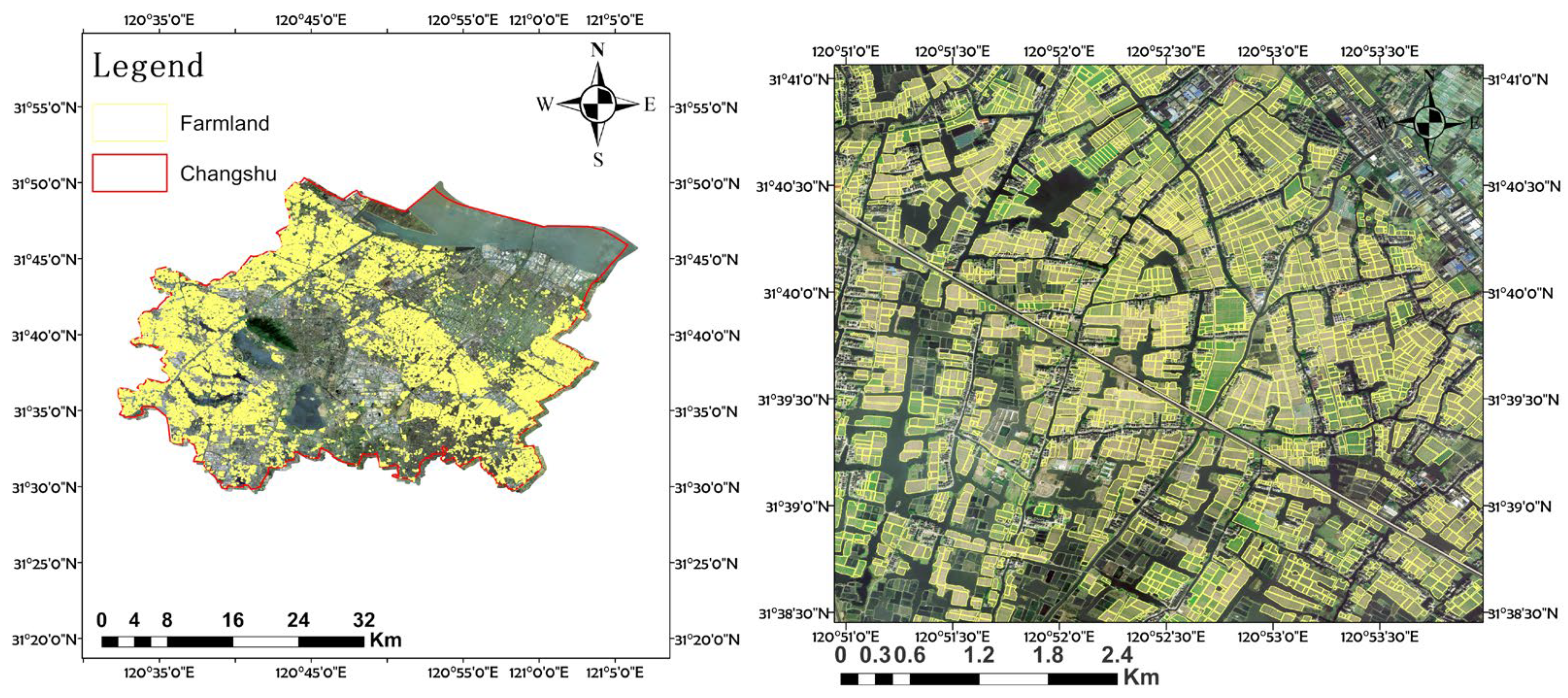
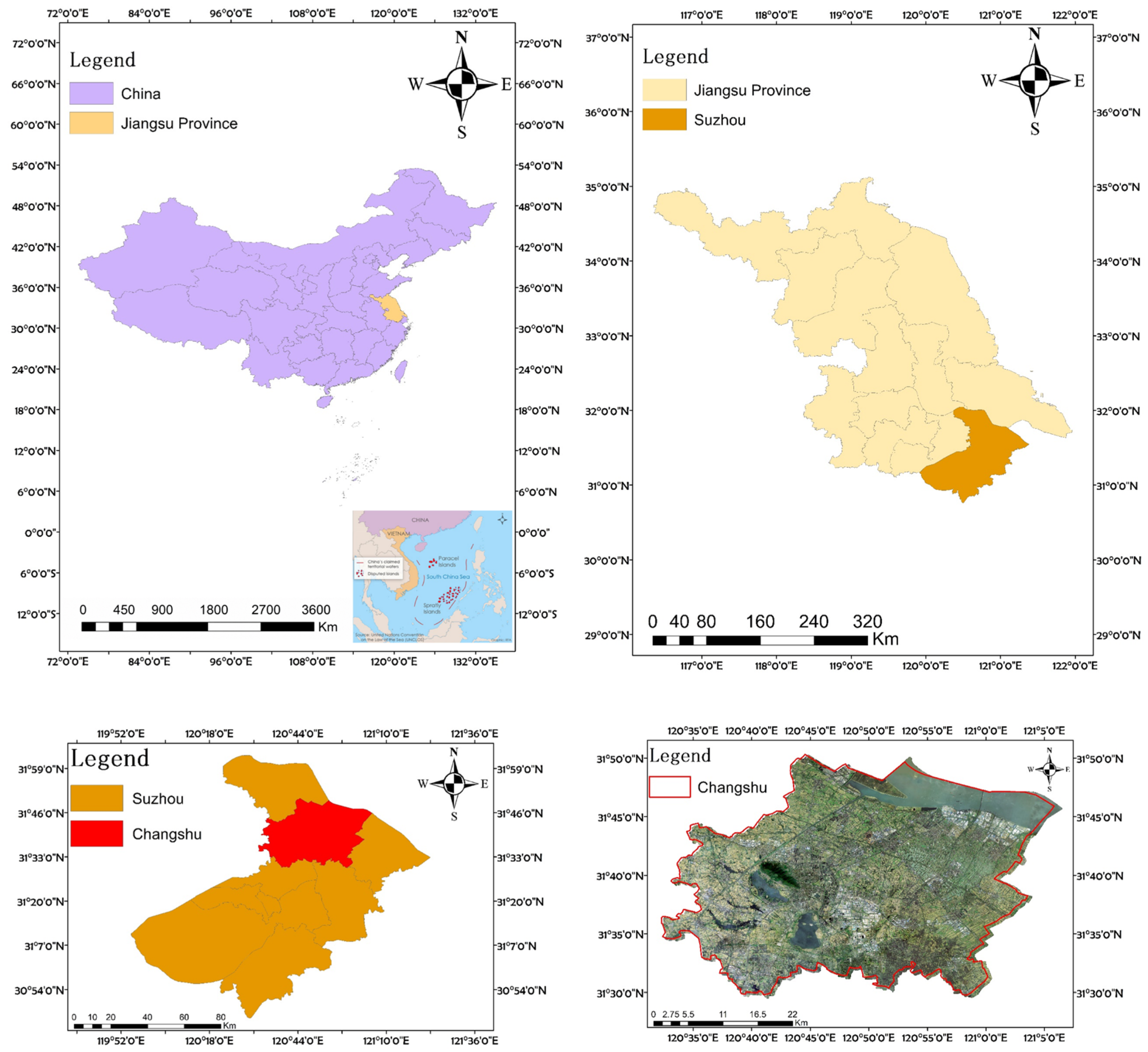
The study area is Changshu City, Suzhou, Jiangsu Province, China (31°31′–31°50′N, 120°33′–121°03′E), covering a total area of approximately 1276 km². The city is situated on the alluvial plain of the Yangtze River Delta and is characterized by flat terrain. The region has a subtropical monsoon climate, with a mean annual temperature of approximately 15.5 °C and mean annual precipitation exceeding 1000 mm. Due to monsoon influence, cloudy and rainy weather is frequent in summer and autumn, resulting in scarce and irregularly distributed Sentinel-2 observations, which poses a significant challenge to traditional classification methods that rely on regularly spaced time series inputs. This is the direct motivation for incorporating all-weather SAR data (Sentinel-1) and adopting an asynchronous time series modeling strategy in this study.

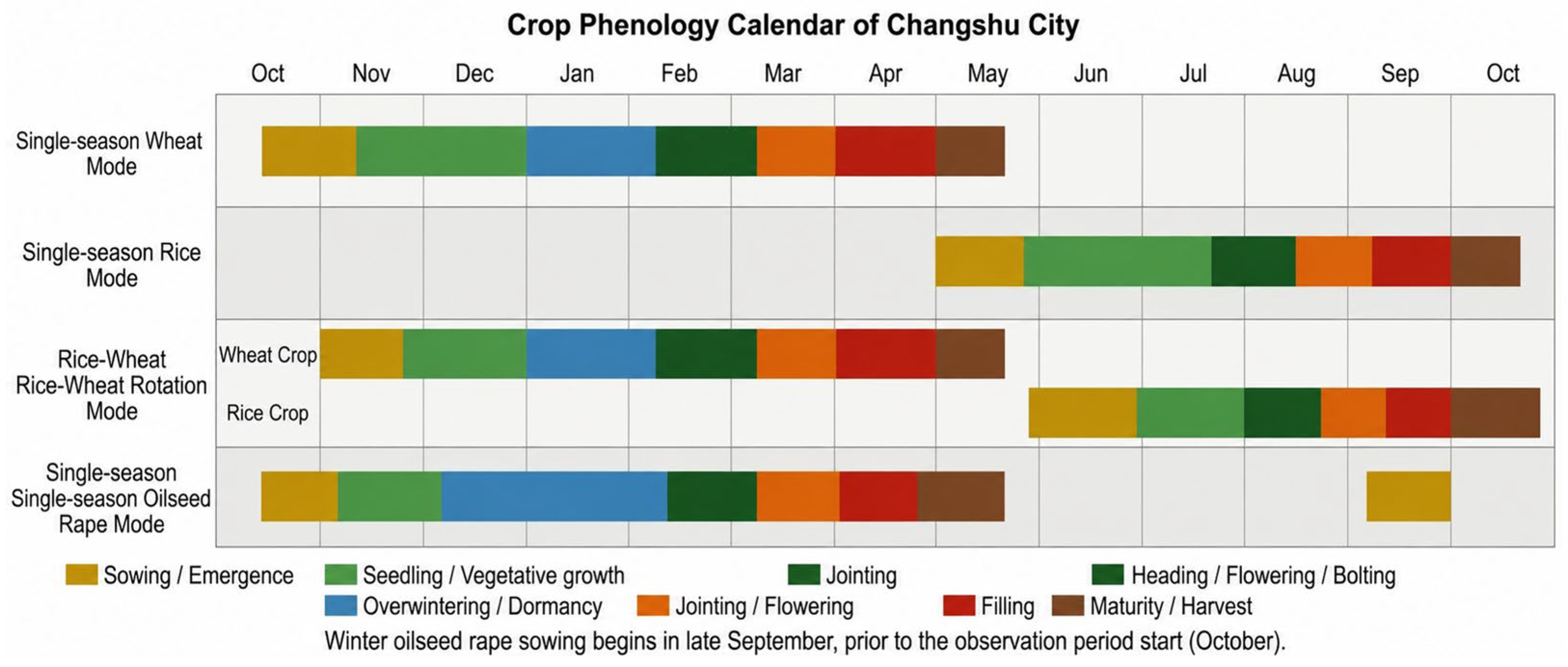
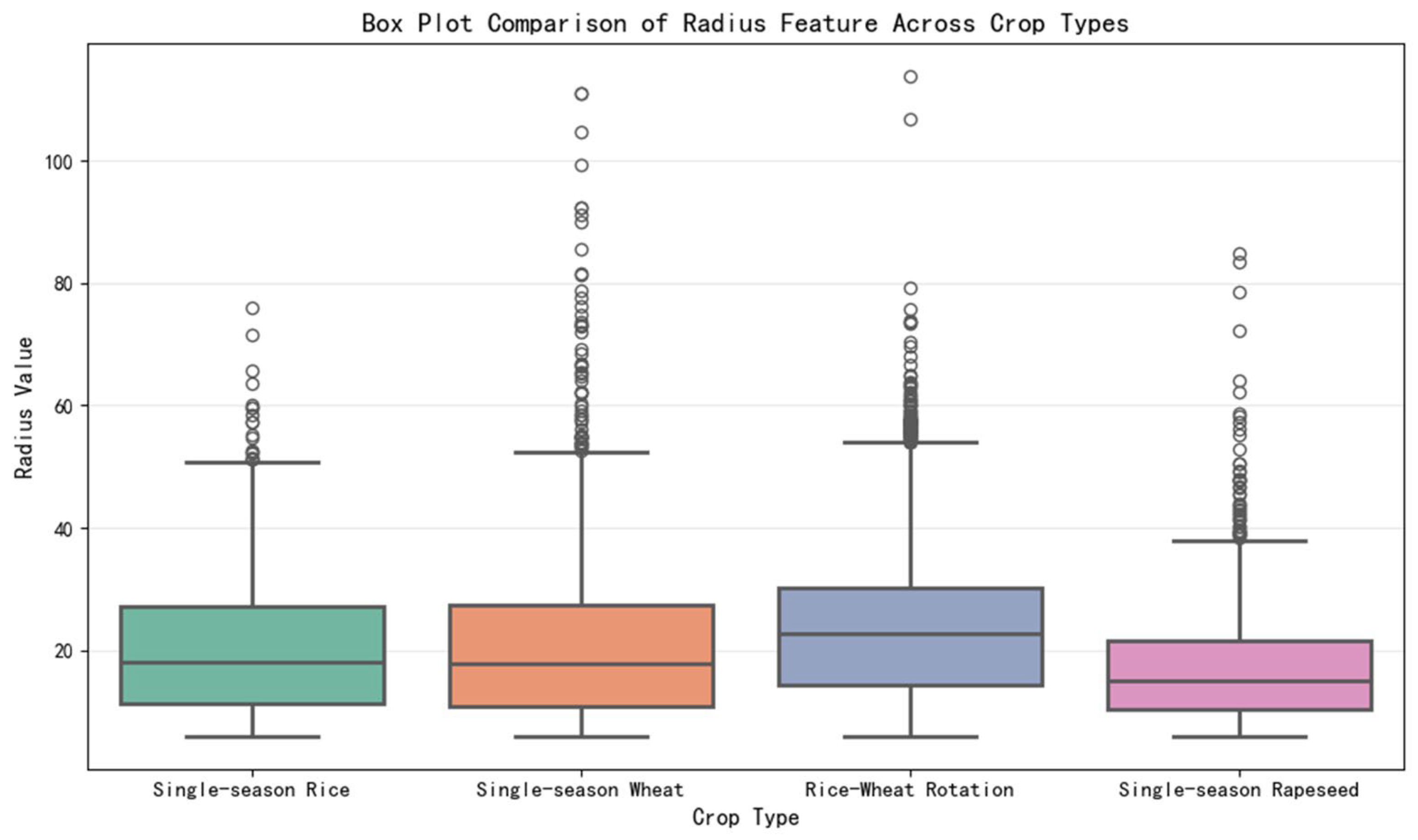
The spatial location and landscape context of the study area are shown in Figure 1. The study area encompasses four major cropping patterns: single-season wheat, single-season rice, rice–wheat rotation, and winter oilseed rape (Figure 2). In terms of agricultural production, Changshu City is a typical smallholder farming area in southern China, characterized by highly fragmented farmland. The median equivalent circular radius of parcels delineated from high-resolution imagery is approximately 19 m (median area: ~1134 m²; Figure 3). Based on a 10 m pixel grid, most parcels contain fewer than three pure interior pixels, with the majority of pixels intersecting parcel boundaries, resulting in prominent mixed-pixel effects. Among these, rice–wheat rotation exhibits substantial spectral overlap with single-season rice and single-season wheat in optical imagery, making it the most challenging source of classification confusion in this study.

The high-resolution imagery overlaid with parcel vector boundaries is shown in Figure 4, further illustrating the fragmented agricultural landscape of the study area.

2.2. Earth Observation and Time-Series Data

The dataset used in this study includes Sentinel-1 and Sentinel-2 data from the European Space Agency’s Copernicus program, two-period (April and August) high-resolution remote sensing imagery covering Changshu City, and parcel vector data delineated from the high-resolution imagery. Data preprocessing, including atmospheric correction, cloud filtering, index calculation, and data download, was performed on the Google Earth Engine platform [21].

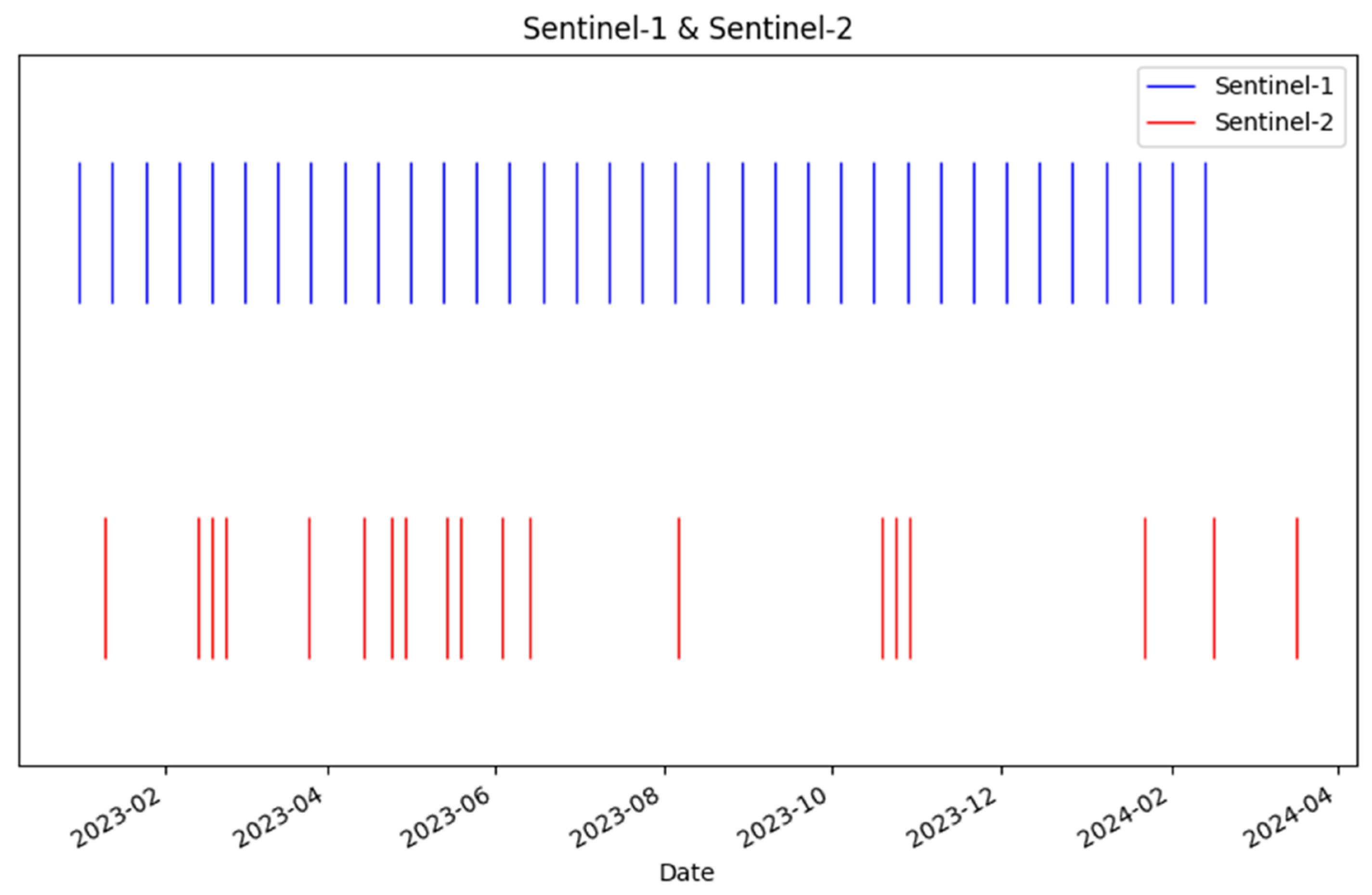
For Sentinel-1, VV, VH, and the VV/VH polarization ratio were selected as input features, yielding 35 acquisition dates from October 2023 to December 2024 (see Figure 5). The SAR data provides all-weather observational capability, enabling cloud-penetrating acquisition of crop phenological signals. For Sentinel-2, bands covering the visible, near-infrared, red-edge, and shortwave infrared regions were selected, yielding 19 acquisition dates over the same period (see

Table 1. Features and calculation methods used in the study.

Satellite Platform	Feature	Formula	Resolution	Resampling
Sentinel-1	VV	-	10 m	-
	VH	-	10 m	-
	Polarization Ratio	VV/VH	10 m	-
Sentinel-2	Blue	-	10 m	-
	Green	-	10 m	-
	Red	-	10 m	-
	Red Edge1	-	20 m → 10 m	Bilinear Interpolation
	Red Edge 2	-	20 m → 10 m	Bilinear Interpolation
	Red Edge 3	-	20 m → 10 m	Bilinear Interpolation
	Near-Infrared	-	10 m	-
	Red Edge 4	-	20 m → 10 m	Bilinear Interpolation
	SWIR (Shortwave Infrared) 1	-	20 m → 10 m	Bilinear Interpolation
	SWIR 2	-	20 m → 10 m	Bilinear Interpolation
Jilin-1 02F	Blue	-	0.8 m	-
	Green	-	0.8 m	-
	Red	-	0.8 m	-

for details). These bands provide rich spectral information for characterizing crop growth stages across different phenological windows. The high-resolution imagery (Jilin-1 02F) has a spatial resolution of 0.8 m, enabling clear delineation of fine parcel boundaries in fragmented landscapes.

2.3. Data Processing

For time series feature extraction, parcel vector masks were applied to preprocessed Sentinel-1 data to extract pure interior pixels. The mean VV and VH backscatter coefficients and the VV/VH ratio were then computed for each acquisition date, yielding a Sentinel-1 time series feature set of 35 dates × 3 features. The same procedure was applied to Sentinel-2 data, yielding a time series feature set of 19 dates × 10 features. The red-edge and SWIR bands, originally at 20 m resolution, were resampled to 10 m via bilinear interpolation on the Google Earth Engine platform during preprocessing. For parcel-level feature extraction, only pure interior pixels within each parcel mask were used, and the per-date mean over these pixels was computed; averaging over pure interior pixels suppresses the influence of residual boundary mixed pixels. For the smallest parcels, which often contain fewer than three pure interior pixels at 10 m resolution, this averaging cannot fully resolve intra-parcel mixed-pixel effects, which motivates the high-resolution image branch.

For high-resolution imagery processing, a 64 × 64 pixel square patch was cropped centered on the geometric centroid of each parcel, normalized to the [0, 1] range, and resized to 224 × 224 pixels to match the input requirement of the ConvFormer_s18 backbone. Two high-resolution patches per parcel (April and August) were retained to provide fine-scale spatial details at the parcel level, including crop canopy structure and field pattern characteristics.

The parcel vector boundaries and initial cropping pattern labels used in this study were both obtained from a government-commissioned agricultural survey project. The parcel boundaries were delineated from the 0.8 m Jilin-1 02F high-resolution imagery as part of that project, with each parcel assigned a unique identifier. The initial cropping pattern labels were derived from governmental agricultural archive records for the 2023 growing season, recorded at the parcel level by local agricultural authorities and linked to the parcel boundaries through shared identifiers. As these labels are administrative records rather than field-verified ground truth, inter-annual cropping pattern changes introduce label noise, which motivates the quality control procedure described in Section 2.5. The initial cropping pattern labels were derived from agricultural archive records of the preceding year, which document cropping patterns at the parcel level and thus naturally align with the spatial granularity of the parcel-level classification task in this study. However, due to inter-annual cropping pattern changes, the actual phenological trajectories of some parcels are inconsistent with their nominal archive labels, representing a typical noisy label scenario. Details of the quality control procedure are provided in Section 2.5.

2.4. Overall Workflow

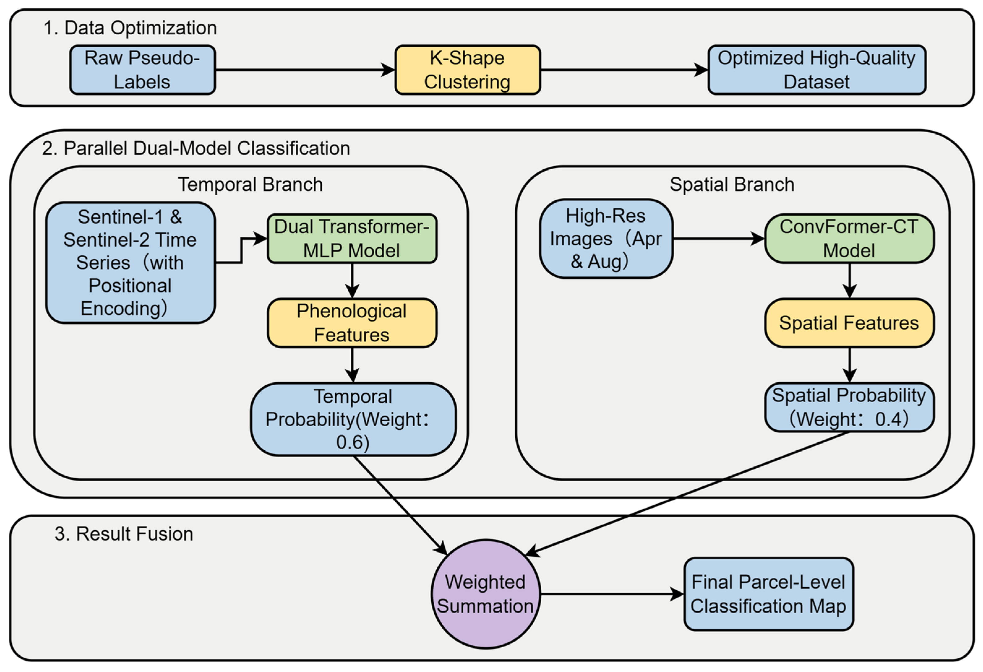
The proposed crop classification framework follows a core logic of data quality control, parallel dual-branch classification, and decision-level fusion. Building on this, the temporal classification model (DualTransformer-MLP (Multi-Layer Perceptron), DT) and the image classification model (ConvFormer-CT) are trained in parallel on the quality-controlled training samples. The temporal branch centers on an asynchronous spatiotemporal Transformer to capture cross-modal phenological dynamics from Sentinel-1 SAR and Sentinel-2 optical data without mandatory temporal alignment, while the image branch employs a class-level attention ConvFormer to extract canopy texture and spatial structural features from 0.8 m high-resolution imagery. Finally, a weighted fusion strategy is applied to combine the predicted probabilities of the two branches through decision-level fusion. The two branches are optimized independently, as the semantic heterogeneity between temporal dynamic features and static spatial texture makes joint end-to-end training prone to gradient imbalance and suppression of the weaker modality.

The asymmetric weights (0.6 for the temporal branch and 0.4 for the image branch) reflect the dominant role of phenological time series features in cropping pattern identification, while high-resolution spatial details serve as a targeted modular complement in partially addressing boundary mixed pixels and disambiguating easily confused patterns in small parcels.

It should be noted that, although K-Shape quality control substantially reduces label noise, it cannot guarantee the complete elimination of residual noisy samples. The dual-branch architecture of PAST offers natural complementarity in this regard: the two branches model independently based on time series phenological signals and high-resolution spatial texture, respectively—the former capturing cross-seasonal crop phenological dynamics and the latter extracting intra-parcel spatial texture. Given the fundamental difference in their feature semantics, the probability of both branches producing identical errors on the same noisy label is low. Therefore, decision-level fusion can partially cancel out the bias introduced by noisy labels in each branch, providing further robustness against residual noisy labels. The overall workflow of the framework is illustrated in Figure 6.

2.5. Sample Quality Control

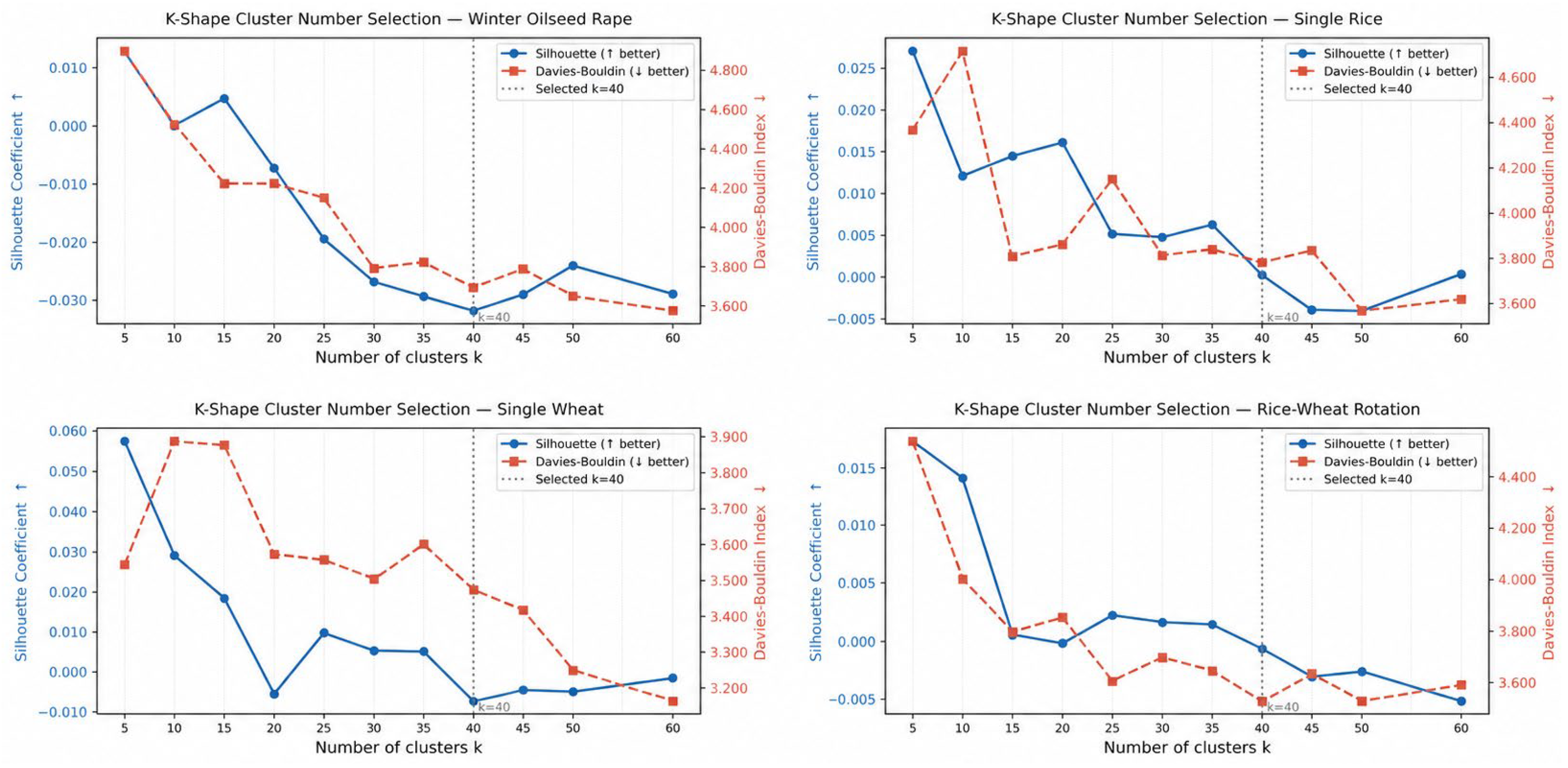
To quantitatively assess the sensitivity of clustering results to the choice of k, we evaluated silhouette coefficients and Davies–Bouldin (DB) indices across k values ranging from 5 to 60 for all four crop classes (Figure 7). Silhouette coefficients remained close to zero across the tested k range and did not exhibit a clear optimum, which is expected given the inherently high intra-class temporal variability of agricultural time series—a characteristic that motivates the use of clustering-based label quality control in the first place. In contrast, the DB index exhibits a clear decreasing trend with increasing k, indicating progressively improved intra-cluster compactness. However, the reduction in DB index becomes progressively smaller beyond k ≈ 40 for most crop classes, suggesting diminishing returns from further increasing k, suggesting that further increases yield only marginal gains. More importantly, excessively large k values produce sub-clusters whose time-series morphologies become phenologically indistinguishable, undermining the interpretability required for domain-expert verification. Considering both the plateau in quantitative improvement and the requirement for phenologically meaningful sub-clusters, k = 40 was selected as a practical balance between clustering granularity and expert reviewability.

Each sub-cluster was then assessed by a single domain expert through a three-step manual review against the following fixed criteria: (1) comparing the mean VV time series curve of each sub-cluster against documented backscatter response characteristics for each crop phenological stage; (2) examining the internal consistency of time series curves within the same cluster; and (3) verifying the spatial texture similarity of co-clustered samples against 0.8 m high-resolution imagery. Sub-clusters passing all three steps were retained as high-confidence samples, while those exhibiting clear deviations in any step were discarded entirely (e.g., double-peak structures appearing in single-season rice sub-clusters, or the absence of a distinct winter trough in winter wheat sub-clusters). After quality control, 8600 high-confidence samples were retained for the rice–wheat rotation class, and 1000–1100 for each of the remaining three classes. To prevent class imbalance from impairing model learning on minority classes, the rice–wheat rotation class was randomly downsampled to 1300 samples. Although class-weighted cross-entropy loss is a common alternative, we found that with a sample ratio exceeding 8:1, downsampling combined with standard cross-entropy yielded more stable convergence and better generalization on the validation set. A final balanced dataset of 4500 samples across all four cropping patterns was therefore adopted for model training. (see

Table 2. Sample quantity per cropping pattern.

Cropping Pattern	Original Count	After QC (Quality Control)	Final Dataset
Single Wheat	3300	1100	1100
Single Rice	6000	1000	1000
Rice–Wheat Rotation	45,000	8600	1300
Winter Oilseed Rape	3300	1100	1100
Total	57,600	11,800	4500

). The substantial discrepancy between the original archive sample counts and the quality-controlled sample counts across classes indirectly reflects the considerable proportion of noisy labels in historical archive records under inter-annual change scenarios, confirming the necessity of the quality control procedure.

2.6. Temporal Classification Model

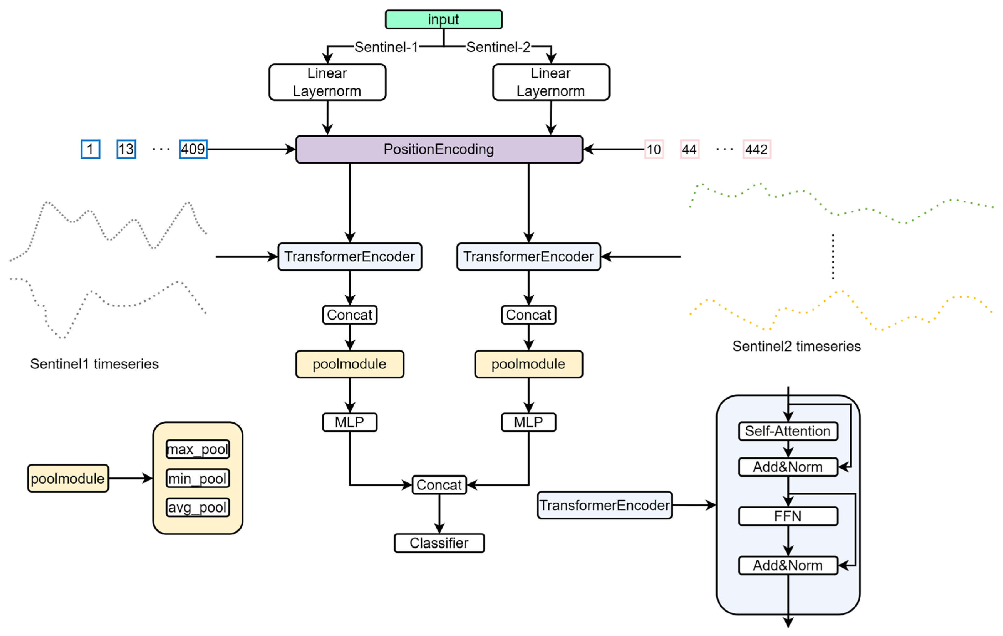
The overall architecture of the temporal classification model (DualTransformer-MLP, DT), illustrated in Figure 8, follows a design pipeline of asynchronous multimodal embedding, dual-path Transformer encoding, multi-dimensional pooling compression, and cross-modal fusion classification, enabling joint exploitation of phenologically discriminative features [22] from SAR and optical time series without mandatory temporal alignment.

2.6.1. Asynchronous Multimodal Temporal Embedding

The Sentinel-1 time series input $X_{\mathrm{sar}}\in {\mathbb{R}}^{L_{\mathrm{sar}}\times C_{\mathrm{sar}}}$ (35 dates, 3 feature channels) and the Sentinel-2 time series input $X_{\mathrm{opt}}\in {\mathbb{R}}^{L_{\mathrm{opt}}\times C_{\mathrm{opt}}}$ (19 dates, 10 feature channels) are each projected into a shared high-dimensional feature space through independent linear transformation layers, followed by Layer Normalization [23] to correct for feature distribution shifts caused by differences in measurement units and dynamic ranges between the two sensors.

Conventional positional encoding uses discrete sequence indices (1, 2, 3…) as positional information, which implicitly assumes uniform temporal spacing between observations. When applied to asynchronous multi-source inputs where the actual time intervals between observations vary substantially, this assumption breaks down and the model loses the ability to perceive true temporal distances. The positional encoding (PositionEncoding) module is the core design of this stage (the central purple module in Figure 8). Rather than following the conventional practice of using sequence indices as positional information, the model directly takes the actual observation date (day of year, DOY) as input to drive the sine–cosine positional encoding. As shown in Figure 8, the observation timestamp sequences of Sentinel-1 and Sentinel-2 are 1, 13,…, 409 and 10, 44,…, 442, respectively, both recorded in days elapsed since the start of the observation period. The sequences differ in length and values, faithfully reflecting the asynchronous and non-uniform sampling characteristics of the two satellites.

The positional encoding is formulated as:

$$\mathrm{PE}(t, 2i)=\mathrm{s}\mathrm{i}\mathrm{n}\left({\displaystyle \frac{t}{{\tau }^{2i/D}}}\right),\mathrm{PE}(t, 2i+1)=\mathrm{c}\mathrm{o}\mathrm{s}\left({\displaystyle \frac{t}{{\tau }^{2i/D}}}\right)$$

(1)

where t is the timestamp of the current observation, D is the feature dimension, i is the dimension index, and τ is the frequency scaling base, set to the standard value of τ = 10,000 in this study. This strategy enables cross-modal phenological learning without interpolation or temporal resampling. The positional encoding vectors are added to the corresponding linear embedding features to obtain the temporally aware input representations ${\tilde{F}}_{\mathrm{sar}}$ and ${\tilde{F}}_{\mathrm{opt}}$ for each modality.

2.6.2. Dual-Branch Transformer Encoding

${\tilde{F}}_{\mathrm{sar}}$ and ${\tilde{F}}_{\mathrm{opt}}$ are fed into two independent Transformer encoders [12] (as illustrated in the enlarged view on the right of Figure 8: Self-Attention [24] → Add&Norm → FFN (Feed-Forward Network) → Add&Norm). Each encoder applies multi-head self-attention to capture long-range phenological dependencies within the modality. The two encoders are kept entirely independent to preserve modality-specific phenological features without inter-modal interference.

2.6.3. Multi-Pooling Compression and MLP Refinement

The outputs of the two Transformer encoders are fed into respective pooling modules (pool module in the lower left of Figure 8: max pooling, min pooling, and average pooling). The three pooling operations compress the temporal dimension from complementary statistical perspectives [25]. The three pooling outputs are concatenated and fed into modality-specific MLPs for feature refinement and dimensionality reduction, compressing the representations to $F_{\mathrm{sar}}^{\mathrm{ref}}\in {\mathbb{R}}^{B\times 64}$ and $F_{\mathrm{opt}}^{\mathrm{ref}}\in {\mathbb{R}}^{B\times 64}$, respectively, while retaining core discriminative information and eliminating redundant dimensions.

2.6.4. Cross-Modal Fusion and Classification Output

The two refined feature vectors are concatenated into a cross-modal fusion feature $F_{\mathrm{fusion}}\in {\mathbb{R}}^{B\times 128}$ and fed into a fully connected classifier, which outputs class prediction probabilities through linear mapping followed by Softmax normalization, completing the cropping pattern classification. The concatenation strategy preserves modality-specific phenological features while reinforcing cross-modal associations through feature complementarity, avoiding the curse of dimensionality that would arise from directly fusing high-dimensional features.

2.6.5. Temporal Branch Loss Function

The temporal branch is trained independently using standard cross-entropy loss. For a batch containing N samples and C classes, the loss function is defined as:

$${\mathcal{L}}_{\mathrm{CE}}^{\mathrm{time}}=-{\displaystyle \frac{1}{N}}{\displaystyle \sum _{i=1}^N}{\displaystyle \sum _{c=1}^C}{y}_{i,c}\mathrm{l}\mathrm{o}\mathrm{g}{p}_{i,c}$$

(2)

The temporal branch jointly encodes and fuses Sentinel-1 and Sentinel-2 inputs within a single model to output unified classification probabilities, and is trained end-to-end using the standard cross-entropy loss ${\mathcal{L}}_{\mathrm{CE}}^{\mathrm{time}}$. Here, $y_{i,c}$ is the class indicator and $p_{i,c}$ is the predicted probability that sample $i$ belongs to class $c$.

2.7. Image Classification Model

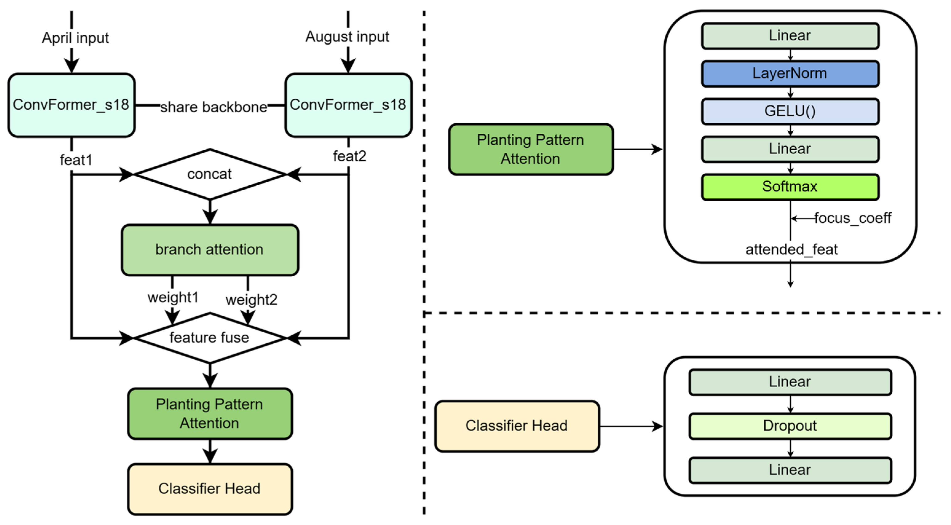
The image classification model adopts ConvFormer-CT (based on the MetaFormer backbone proposed by Yu et al. [26]) as its backbone to extract spatial features from the two-period high-resolution imagery through a shared backbone network. Combined with branch attention fusion and a planting pattern attention module, it provides complementary parcel-level spatial texture information for the temporal branch.

2.7.1. Shared-Backbone Dual-Branch Feature Extraction

The model takes high-resolution imagery from two periods—April and August—as input. These two periods capture a complementary canopy-presence contrast among the dominant crops: in April, winter wheat (jointing) and oilseed rape (bolting–flowering) exhibit well-developed canopies while rice paddies are not yet transplanted; in August, rice (heading–grain-filling) is in vigorous growth while wheat and rape have already been harvested. The two periods share the same ConvFormer_s18 [26] backbone weights, which has approximately 26 M parameters. This variant offers a low risk of overfitting under limited sample conditions while retaining sufficient feature extraction capacity, making it well-suited for transfer learning fine-tuning in the remote sensing scenario of this study. Spatial features F_“apr” ∈R^(B × C × H × W) (feat1) and F_“aug” ∈R^(B × C × H × W) (feat2) are extracted for the April and August periods, respectively.

Weight sharing ensures a consistent feature space between the two periods while reducing model parameters and overfitting risk.

2.7.2. Branch Attention Adaptive Fusion

Different cropping patterns exhibit fundamentally different dependencies on the two periods: single-season rice identification relies more heavily on canopy characteristics during the heading–grain-filling stage in August, single-season wheat depends primarily on its well-developed canopy during the jointing stage in April, and rice–wheat rotation draws on both periods simultaneously. To adaptively learn the weight allocation between the two periods for each sample, the model incorporates a Branch Attention module.

Specifically, feat1 and feat2 are concatenated along the channel dimension and fed into the Branch Attention module, which generates two adaptive fusion weights $w_1$ and $w_2$ (satisfying $w_1+w_2=1$). The two-period features are then combined through weighted summation:

$$F_{\mathrm{fuse}}=w_1\cdot F_{\mathrm{apr}}+w_2\cdot F_{\mathrm{aug}}$$

(3)

This mechanism enables the model to dynamically adjust the contribution of each period for different samples, rather than relying on fixed weights or implicitly handling temporal fusion through convolutional layers after channel concatenation, thereby more precisely capturing the key phenological stage features of each cropping pattern.

2.7.3. Planting Pattern Guided Attention

The fused feature $F_{\mathrm{fuse}}$ is further processed by a Planting Pattern Attention module. For the three easily confused classes—single-season rice, single-season wheat, and rice–wheat rotation—whose phenological characteristics are highly overlapping, the module explicitly enhances their discriminative weights through learnable class-specific focus coefficients. The internal structure of the module (upper right of Figure 9) follows the sequence: Linear → LayerNorm [23] → GELU (Gaussian Error Linear Unit) [27] → Linear → Softmax. The resulting class attention distribution is multiplied by a trainable focus coefficient focus_coeff to directionally enhance the attention weights of easily confused classes, ultimately outputting the attention-enhanced feature attended_feat:

$$\mathrm{attended}\_\mathrm{feat}=\mathrm{focus}\_\mathrm{coeff}\odot \mathrm{Softmax}(W_2·\mathrm{GELU}(\mathrm{LN}(W_1{F}_{\mathrm{fuse}})))·F_{\mathrm{fuse}}$$

(4)

This mechanism directs the model’s attention toward spatial texture differences among the three phenologically similar classes (single-season rice, single-season wheat, and rice–wheat rotation), improving discrimination accuracy for these easily confused patterns.

2.7.4. Classification Head

The attended_feat is fed into the classification head (Linear → Dropout → Linear), as illustrated in the lower right of Figure 9. The intermediate Dropout layer randomly deactivates a subset of neurons during training to suppress overfitting under limited sample conditions and improve generalization. The final fully connected layer maps the features to the target number of classes, outputting the predicted logits for each class.

2.7.5. Image Branch Loss Function

The image branch is also trained independently using standard cross-entropy loss:

$${\mathcal{L}}_{\mathrm{CE}}^{\mathrm{img}}=-{\displaystyle \frac{1}{N}}{\displaystyle \sum _{i=1}^N}{\displaystyle \sum _{c=1}^C}{y}_{i,c}\mathrm{l}\mathrm{o}\mathrm{g}{p}_{i,c}$$

(5)

The symbol definitions are consistent with those of the temporal branch.

2.8. Experimental Setup

2.8.1. Dataset Partitioning and Evaluation Metrics

The experimental dataset comprises 4500 samples across four cropping patterns, split into training (2963 samples), validation (741 samples), and test (796 samples) sets, with class proportions kept consistent across all splits. Macro-averaged precision, recall, and F1 score are adopted as the primary evaluation metrics to comprehensively reflect model performance under class imbalance conditions.

To evaluate model performance on small parcels specifically, test set parcels are divided into small parcels (inscribed circle radius < 20 m) and large parcels; the inscribed circle radius is adopted as the size metric because it captures the narrowest dimension of each parcel, which directly determines the severity of mixed-pixel effects along parcel boundaries. The small-parcel subset contains 467 samples and the large-parcel subset contains 329 samples.

2.8.2. Baseline Models

The time series baselines include LSTM [6], TCN [7], Rocket [28], PatchTST [29], and InceptionTime [30], all of which take the same multimodal time series features (Sentinel-1 and Sentinel-2) as input to ensure fair comparison. The image baselines include CNN (a custom three-layer convolutional baseline with batch normalization and max-pooling, followed by fully connected layers), ViT (Vision Transformer) [31], and ResNet50 [32], all taking the same two-period high-resolution imagery as input. To ensure a fair comparison, all time-series baselines were trained under the same data partition and training protocol as our temporal branch, and all image baselines under the same protocol as our image branch. The key configurations of all baseline models are summarized in

Table 3. Baseline model configurations.

Model	Learning Rate	Batch Size	Optimizer	Epochs	Early-Stop Patience
LSTM	5 × 10−3	68	AdamW (wd 4 × 10−3)	200	10
TCN	5 × 10−3	68	AdamW (wd 4 × 10−3)	200	10
PatchTST	5 × 10−3	68	AdamW (wd 4 × 10−3)	200	10
Rocket	-	-	-	-	-
InceptionTime	5 × 10−3	68	AdamW (wd 4 × 10−3)	200	10
CNN	1 × 10−5	68	AdamW (wd 5 × 10−4)	200	10
ViT	1 × 10−5	256	AdamW (wd 5 × 10−4)	200	10
ResNet50	1 × 10−5	68	AdamW (wd 5 × 10−4)	200	10

.

2.8.3. Hyperparameters

All models are implemented in Python 3.10 using PyTorch 2.1.0 with CUDA 11.8 [33]. The key hyperparameters are summarized in

Table 4. Hyperparameter settings for both branches.

Hyperparameter	Time-Series Branch	Image Branch
Optimizer	AdamW	AdamW
Learning rate	5 × 10−3	1 × 10−5
Weight decay	4 × 10−3	5 × 10−4
Batch Size	68	256
Dropout	0.3	-
LR schedule	ReduceLROnPlateau	CosineAnnealingWarmRestarts
Max epochs	200	200
Early-stop patience	10	15
Input size	S1 seq = 35, S2 seq = 19	224 × 224 px
Data augmentation	-	Flip/Rot (±15°)/ColorJitter
Loss function	CrossEntropyLoss	Weighted CrossEntropyLoss

. The temporal branch employs a two-layer stacked Transformer encoder with a hidden dimension of 32, 8 attention heads, and a feed-forward dimension of 64, incorporating DOY-based sine–cosine positional encoding to handle asynchronous irregular inputs. The optimizer is AdamW [34], paired with a ReduceLROnPlateau learning rate scheduler with linear warmup (3 warmup epochs, decay factor 0.5).

The image branch uses ImageNet-pretrained ConvFormer_s18 as the backbone, with the first three stages frozen and only the last stage and classification head fine-tuned, preserving general visual features while adapting to the remote sensing scenario. Training data augmentation includes random flipping, rotation (±15°), and color jitter. To address class imbalance, a combination of weighted random sampling and weighted cross-entropy loss is adopted.

Both branches are trained for a maximum of 200 epochs with early stopping based on validation loss.

To evaluate computational efficiency, the model parameters, inference latency, and training time of PAST are summarized in

Table 5. Model efficiency of PAST, measured on a single NVIDIA GTX 1080 Ti GPU (NVIDIA Corporation, Santa Clara, CA, USA).

Component	Parameters	Trainable Params	Inference Latency (ms/sample)	Training Time
Temporal branch	61,812	61,812	0.12	19.6 s
Image branch	24,725,974	8,501,270	11.31	3.7 h
Full PAST	≈24.79 M	≈8.56 M	≈11.43	≈3.7 h

.

The temporal branch is extremely lightweight (≈0.06 M parameters, 0.12 ms per sample, under 20 s of total training), while the image branch—built on the ConvFormer_s18 backbone with its first three stages frozen—contains ≈ 24.7 M parameters (8.5 M trainable) and requires approximately 3.7 h of training. As the two branches are optimized independently and combined through decision-level fusion, the end-to-end single-sample inference latency of the full framework is approximately 11.4 ms. These results indicate that, despite its dual-branch design, PAST remains computationally modest and can be trained and deployed on a single consumer-grade GPU, which is favorable for operational mapping workflows.

3. Results

3.1. Time-Series Branch and Image Branch Performance Comparison

3.1.1. Time-Series Model Comparison

The proposed temporal branch achieves the best performance across all parcels (F1 = 0.915). Compared to LSTM and TCN, which rely on uniformly spaced inputs, the proposed method directly handles the asynchronous and non-uniform timestamps of Sentinel-1 and Sentinel-2 through DOY-based sine–cosine positional encoding, effectively preserving abrupt short-term signals during critical phenological stages such as jointing and heading. The dual independent Transformer encoders and triple pooling further ensure comprehensive extraction of cross-modal phenological features. LSTM achieves the lowest performance (F1 = 0.866), fundamentally because it relies on sequential order to implicitly encode temporal information and cannot handle irregular observation intervals.

The all-parcel time-series model comparison results are summarized in

Table 6. Time-series comparison of all parcels.

Model	Precision	Recall	F1
LSTM	0.866	0.867	0.866
TCN	0.914	0.907	0.910
Rocket	0.903	0.899	0.901
InceptionTime	0.866	0.871	0.868
PatchTST	0.905	0.894	0.899
Ours-Time Series Branch Only	0.924	0.909	0.915

.

The corresponding small-parcel comparison results are shown in

Table 7. Comparison of time-series models for small parcels.

Model	Precision	Recall	F1
LSTM	0.836	0.818	0.820
TCN	0.894	0.881	0.886
Rocket	0.872	0.870	0.870
InceptionTime	0.842	0.846	0.843
PatchTST	0.864	0.851	0.856
Ours-Time Series Branch Only	0.899	0.882	0.889
Ours-Full Model	0.921	0.898	0.906

.

In the small-parcel scenario, all models experience performance degradation. The full model F1 drops from 0.926 to 0.906 (a decrease of 2.0 percentage points), the temporal branch alone drops from 0.915 to 0.889 (2.6 percentage points), and the second-best TCN drops from 0.910 to 0.886 (2.4 percentage points). Notably, the performance gain from adding the image branch is more pronounced in the small-parcel scenario (0.889 → 0.906) than in the all-parcel scenario (0.915 → 0.926), indicating that spatial texture features provide complementary information in fragmented small parcels.

3.1.2. Image Model Comparison

The image branch achieves lower overall performance than the temporal branch, which is consistent with the nature of the task—the primary basis for cropping pattern discrimination is annual phenological dynamics, which static imagery cannot fully capture across seasons. This represents a fundamental limitation shared by all image-based models. The proposed ConvFormer-CT achieves the best performance among image-based models (F1 = 0.719), with the adaptive weight fusion of the Branch Attention module and the directional focusing of the Planting Pattern Attention module being the key contributing factors. ResNet50 achieves the lowest performance (F1 = 0.450), as the absence of any temporal association design prevents it from distinguishing cropping patterns that rely on cross-seasonal feature evolution. The all-parcel image model comparison results are summarized in

Table 8. Image comparison of all parcels.

Model	Precision	Recall	F1
CNN	0.603	0.599	0.591
ResNet50	0.507	0.470	0.450
ViT	0.686	0.680	0.678
Ours-Image Branch Only	0.724	0.718	0.719

.

The corresponding small-parcel image model comparison results are shown in

Table 9. Comparison of image models for small parcels.

Model	Precision	Recall	F1
CNN	0.567	0.555	0.551
ResNet50	0.531	0.450	0.441
ViT	0.658	0.630	0.636
Ours-Image Branch Only	0.681	0.666	0.670
Ours-Full Model	0.921	0.898	0.906

.

In the small-parcel scenario, all image-based models experience larger performance drops than time series models, with the image branch alone declining from 0.719 to 0.670 (a decrease of 4.9 percentage points), further indicating that purely image-based methods have limited robustness against boundary mixed-pixel effects in fragmented parcels. The full fusion model still achieves an F1 of 0.906 in the small-parcel scenario, outperforming the image branch alone by 23.6 percentage points, demonstrating that temporal phenological information is an indispensable core support for fragmented parcel classification, with the image branch providing targeted complementary information.

3.2. Fusion Strategy Comparison and Final Results

Three-modal feature-level fusion refers to directly concatenating the extracted features from three modalities—Sentinel-1 time series, Sentinel-2 time series, and high-resolution imagery—and feeding the concatenated feature vector into a single classifier.

Decision-level fusion significantly outperforms feature-level fusion because the fundamental semantic heterogeneity between temporal dynamic features and static spatial texture features causes chaotic feature distributions after direct concatenation, making it difficult for a linear classifier to handle both semantic levels simultaneously. In contrast, decision-level fusion allows each branch to be independently optimized under the objective function best suited to its modality, achieving complementary fusion at the probability level and effectively avoiding interference from cross-modal feature distribution mismatch. The fusion weights (0.6 for the temporal branch and 0.4 for the image branch) are determined through grid search on the validation set, and their asymmetry objectively reflects the dominant role of phenological time series features in cropping pattern identification. The comparison results of different fusion strategies are summarized in

Table 10. Comparison of different fusion strategies.

Fusion Strategies	Precision	Recall	F1
Three-modal Fusion	0.833	0.810	0.814
Decision-level Fusion	0.936	0.919	0.926

.

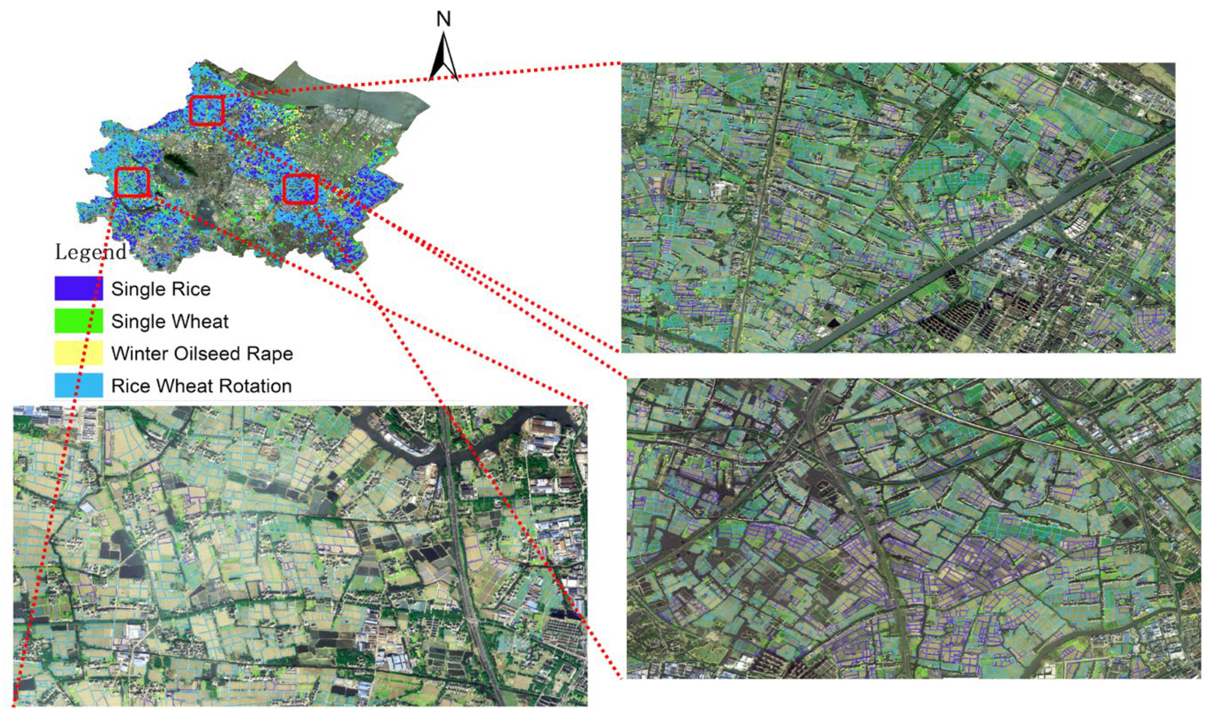
The final crop classification map generated by the proposed PAST framework is shown in Figure 10.

3.3. Ablation Study

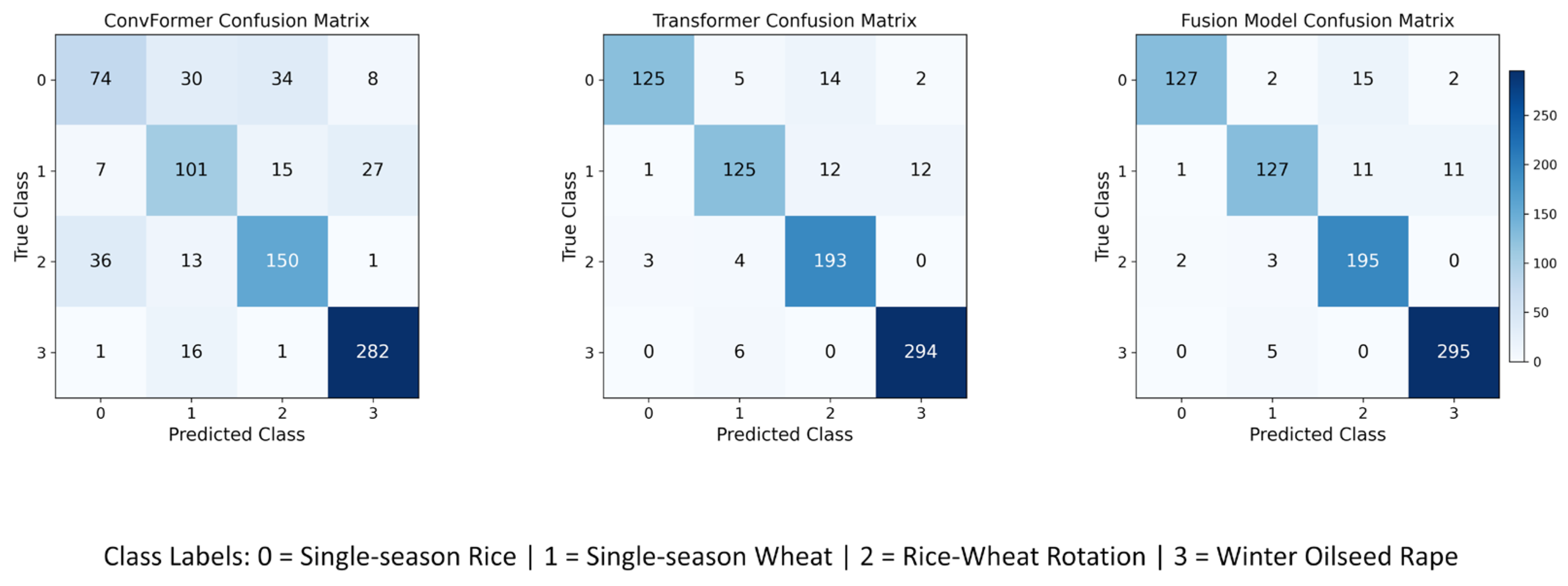
The ablation results and confusion matrices (Figure 11) jointly validate the effectiveness of the dual-branch fusion mechanism. Removing the image branch causes F1 to drop from 0.926 to 0.915, with performance degradation primarily concentrated in mutual confusion between single-season rice and rice–wheat rotation and misclassification of boundary parcels, indicating that 0.8 m high-resolution texture features provide a complementary role in spatial anchoring of fragmented parcels. Removing the temporal branch causes F1 to drop substantially to 0.719, with single-season rice recall falling to only 0.507, as a large number of samples are misclassified into the visually similar rice–wheat rotation class in August, confirming that annual phenological time series features are an irreplaceable core discriminative basis for cropping pattern identification. The ablation results for the three model configurations are summarized in

Table 11. Ablation experiment.

	Precision	Recall	F1
Image Branch Only	0.724	0.718	0.719
Time-Series Branch Only	0.924	0.909	0.915
Full Dual-Branch Model	0.936	0.919	0.926

.

3.4. Ablation Study on Label Quality Control

To validate the effectiveness of K-Shape label quality control, an ablation experiment is conducted using the full PAST framework under two conditions: one trained on 4500 samples randomly drawn from the unfiltered raw label set (containing noisy labels due to inter-annual cropping pattern changes), and one trained on the 4500 quality-controlled samples selected by K-Shape. By fixing the sample size across both conditions, this design isolates label quality as the sole variable, eliminating the confounding effect of sample quantity. The results show that the full model trained on raw labels achieves an F1 of only 0.808, which increases to 0.926 after quality control, representing an improvement of 11.8 percentage points. These results clearly demonstrate that the performance gain stems from the improvement in label quality rather than the reduction in sample size, confirming the critical role of K-Shape quality control in providing a reliable training foundation for the PAST framework. The quantitative results of the label quality control ablation are summarized in

Table 12. Performance comparison with and without label quality control.

	Precision	Recall	F1
w/o QC (Raw Labels)	0.823	0.804	0.808
w/QC (Ours)	0.936	0.919	0.926

.

4. Discussion

4.1. Interpretation of Key Findings

The proposed PAST framework achieves strong classification performance in the Changshu City experiment. Notably, a large proportion of raw archive samples were rejected during K-Shape quality control, which reflects the reliability limitations of historical archive labels under inter-annual cropping change scenarios. This finding suggests that in remote sensing mapping studies relying on historical archives as weakly supervised labels, systematic label quality assessment should be treated as a necessary component of the methodological design.

It is worth noting that the K-Shape-based quality control adopted in this study is an offline hard-filtering mechanism, which differs from emerging fault-tolerant learning strategies such as co-teaching [35] or generalized cross-entropy loss [19], where the network itself learns to suppress noisy gradients during training. The offline approach was chosen here because the label noise originates from a well-defined physical cause—inter-annual cropping pattern changes—which produces coherent, interpretable deviations in the Sentinel-1 VV time series that are amenable to cluster-level human verification. In scenarios where label noise lacks such physical interpretability, or where domain expert review is unavailable, end-to-end noise-tolerant learning strategies would be a more appropriate choice.

4.2. Limitations and Future Directions

Model-level limitations. The current framework employs decision-level fusion, where the two branches are combined only through weighted summation at the probability level. This shallow fusion approach prevents cross-modal feature interaction during the extraction stage, and the fixed fusion weights cannot adapt to the dynamic variation in the relative importance of each modality across different crop types and phenological stages. The ablation results reflect this limitation: the full dual-branch model (F1 = 0.926) outperforms the temporal branch alone (F1 = 0.915) by only 1.1 percentage points, suggesting that the complementary value of spatial features has not yet been fully exploited. Introducing cross-modal attention mechanisms to enable deep feature interaction during the encoding stage represents a natural direction for addressing this bottleneck. In addition, the image branch currently uses only two fixed acquisition periods (April and August), making it difficult to precisely align with the key phenological nodes of each crop type. Expanding the temporal coverage of high-resolution imagery to align the image branch with more key phenological nodes identified from the time series data could further strengthen the spatiotemporal complementarity of the dual-branch design. Furthermore, both branches currently rely on task-specific architectures—an ImageNet-pretrained backbone for the image branch and a Transformer trained from scratch for the temporal branch. Adapting remote-sensing foundation models to this framework—for example, spectral–temporal image foundation models for high-resolution parcel-level texture extraction, and pre-trained temporal models extended to the asynchronous multi-source setting addressed here—represents a promising direction for further improving feature representation. In addition, the temporal branch currently operates on raw Sentinel-2 spectral bands; explicitly incorporating phenology-sensitive vegetation indices (e.g., NDVI, EVI, LSWI)—particularly for distinguishing phenologically overlapping classes such as single-season rice and rice–wheat rotation—represents a further direction for enriching the spectral feature representation.

Data-level limitations. To maintain class balance across the four cropping patterns, the rice–wheat rotation class was downsampled from 8600 post-QC samples to 1300, leaving a substantial portion of high-confidence samples unused and limiting the actual training sample size. The QC rejection rate for this class reaches approximately 81%, substantially higher than other classes, suggesting that historical archive labels for rotation patterns are particularly unreliable and deserve attention in similar studies. Semi-supervised approaches—such as self-training or consistency regularization that leverage the retained high-confidence samples without discarding them—represent a promising direction for making fuller use of the available data. Validating the framework under larger and more geographically diverse sample conditions remains an important direction for assessing its generalizability across different agricultural landscape contexts.

Pipeline scalability. Although the three-step manual review is conducted at the sub-cluster level rather than the sample level—reducing the number of review units from 57,600 raw samples to 160 sub-clusters across four classes, a reduction of more than two orders of magnitude—the scalability of this pipeline to provincial or national operational mapping contexts, where regional phenological diversity and data volume increase substantially, remains a limitation. We further note that the sub-cluster review was conducted by a single expert against the fixed criteria defined in Section 2.5; while these criteria are explicit and physically grounded, a multi-reviewer protocol with inter-reviewer agreement assessment was not conducted. Threshold-based automatic sub-cluster rejection would both improve scalability and remove residual reviewer subjectivity. Replacing manual verification with threshold-based automatic sub-cluster rejection rules, or integrating the pipeline with end-to-end noise-tolerant learning strategies, represents a promising direction for extending the framework to larger geographic scales.

Geographical generalizability. All experiments in this study are conducted in Changshu City, a representative fragmented farmland area in the Yangtze River Delta characterized by flat alluvial terrain and a subtropical monsoon climate. While the methodological challenges addressed by PAST—including cloud interference, asynchronous multi-source observations, and mixed-pixel effects—are broadly relevant to smallholder farming regions across China, the generalizability of the framework to areas with more complex topography, such as the mountainous provinces of Yunnan, Guizhou, or Sichuan where terrain-induced shadow effects and more severe cloud cover may further complicate data acquisition and model performance, has not yet been validated. Extending the evaluation to such geographically diverse settings represents an important direction for future work.

Reproducibility. The high-resolution imagery and parcel-level annotation data used in this study were provided under a government-commissioned project and are subject to data access restrictions. This limits the full reproducibility of the experimental results. However, the Sentinel-1 and Sentinel-2 time-series data are publicly available through Google Earth Engine, the model architecture and training procedures are fully described, and the methodological framework itself is transferable to other study areas where parcel boundaries and initial labels can be obtained from local sources.

5. Conclusions

To address the challenges associated with mixed-pixel effects, observation asynchrony, and complex cropping pattern identification in high-accuracy parcel-level agricultural mapping in fragmented regions of the Yangtze River Delta, this study proposes PAST, a parcel-level cropping pattern classification framework comprising K-Shape-based label quality control, parallel dual-branch classification, and decision-level fusion.

The main conclusions are as follows:

First, the semi-automatic label quality control method based on K-Shape time series clustering effectively filters noisy labels from historical archive records, providing a reliable weakly supervised foundation for model training, and to some extent reflects the reliability limitations of historical archive labels under inter-annual cropping change scenarios.

Second, the asynchronous spatiotemporal Transformer branch directly maps the irregular timestamps of Sentinel-1 and Sentinel-2 onto a shared semantic time axis through DOY-based sine–cosine positional encoding, enabling autonomous learning of cross-modal phenological associations without mandatory alignment, effectively preserving abrupt short-term signals during critical phenological stages such as jointing and heading, and outperforming baseline models that rely on uniformly spaced inputs, including LSTM and TCN, in both all-parcel and small-parcel scenarios.

Third, the class-level attention ConvFormer branch extracts canopy texture and parcel spatial structural features from 0.8 m high-resolution imagery, adaptively learns the fusion weights of the two-period imagery through the Branch Attention module, and incorporates learnable focus coefficients for easily confused classes, achieving the best performance among image-based models and providing targeted complementary spatial anchoring for boundary mixed pixels in fragmented parcels.

Fourth, the decision-level fusion strategy accommodates the semantic heterogeneity between temporal dynamic features and static spatial texture, significantly outperforming the three-modal feature-level fusion strategy based on direct feature concatenation (F1: 0.926 vs. 0.814), validating the effectiveness of complementary fusion at the probability level after independent branch optimization.

Experimental results demonstrate that PAST achieves an overall F1 score of 0.926 and a small-parcel F1 score of 0.906, providing an effective technical solution for fine-grained cropping pattern mapping in fragmented agricultural landscapes.

References

1. Mulla, D.J. Twenty Five Years of Remote Sensing in Precision Agriculture: Key Advances and Remaining Knowledge Gaps. Biosyst. Eng. 2013, 114, 358–371. [Google Scholar] [CrossRef]
2. Wu, W.; Yu, Q.; You, L.; Chen, K.; Tang, H.; Liu, J. Global Cropping Intensity Gaps: Increasing Food Production without Cropland Expansion. Land Use Policy 2018, 76, 515–525. [Google Scholar] [CrossRef]
3. Weiss, M.; Jacob, F.; Duveiller, G. Remote Sensing for Agricultural Applications: A Meta-Review. Remote Sens. Environ. 2020, 236, 111402. [Google Scholar] [CrossRef]
4. Xia, L.; Chen, C.; Luo, J.; Hu, X.; Lu, X.; Yu, H.; Lu, K. A Precise Spatiotemporal Fusion Crop Classification Framework Based on Parcels. Sci. Rep. 2025, 15, 19208. [Google Scholar] [CrossRef] [PubMed]
5. Wang, H.; Wang, J.; Shen, Z.; Zhang, Z.; Li, J.; Zhao, L.; Jiao, S.; Li, S.; Lei, Y.; Kou, W.; et al. Parcel-Level Mapping of Apple Orchard in Smallholder Agriculture Areas Based on Feature-Level Fusion of VHR Image and Time-Series Images. Int. J. Remote Sens. 2022, 43, 6195–6220. [Google Scholar]
6. Rußwurm, M.; Körner, M. Multi-Temporal Land Cover Classification with Sequential Recurrent Encoders. ISPRS Int. J. Geo-Inf. 2018, 7, 129. [Google Scholar] [CrossRef]
7. Pelletier, C.; Webb, G.I.; Petitjean, F. Temporal Convolutional Neural Network for the Classification of Satellite Image Time Series. Remote Sens. 2019, 11, 523. [Google Scholar] [CrossRef]
8. Liu, L.; Cao, R.; Chen, J.; Shen, M.; Wang, S.; Zhou, J.; He, B. Detecting Crop Phenology from Vegetation Index Time-Series Data by Improved Shape Model Fitting in Each Phenological Stage. Remote Sens. Environ. 2022, 277, 113060. [Google Scholar] [CrossRef]
9. Xiao, X.; Boles, S.; Frolking, S.; Li, C.; Babu, J.Y.; Salas, W.; Moore, B., III. Mapping Paddy Rice Agriculture in South and Southeast Asia Using Multi-Temporal MODIS Images. Remote Sens. Environ. 2006, 100, 95–113. [Google Scholar] [CrossRef]
10. Dong, J.; Xiao, X.; Menarguez, M.A.; Zhang, G.; Qin, Y.; Thau, D.; Biradar, C.; Moore, B., III. Mapping Paddy Rice Planting Area in Northeastern Asia with Landsat 8 Images, Phenology-Based Algorithm and Google Earth Engine. Remote Sens. Environ. 2016, 185, 142–154. [Google Scholar] [CrossRef] [PubMed]
11. Hao, S.; Wang, W.; Ye, Y.; Nie, T.; Bruzzone, L. Two-Stream Deep Architecture for Hyperspectral Image Classification. IEEE Trans. Geosci. Remote Sens. 2018, 56, 2349–2361. [Google Scholar] [CrossRef]
12. Rußwurm, M.; Körner, M. Self-Attention for Raw Optical Satellite Time Series Classification. ISPRS J. Photogramm. Remote Sens. 2020, 169, 421–435. [Google Scholar] [CrossRef]
13. Yuan, Y.; Lin, L. Self-Supervised Pretraining of Transformers for Satellite Image Time Series Classification. IEEE J. Sel. Top. Appl. Earth Obs. Remote Sens. 2020, 14, 474–487. [Google Scholar] [CrossRef]
14. Tarasiou, M.; Chavez, E.; Zafeiriou, S. Vits for Sits: Vision Transformers for Satellite Image Time Series. In Proceedings of the IEEE/CVF Conference on Computer Vision and Pattern Recognition; IEEE: Piscataway, NJ, USA, 2023; pp. 10418–10428. [Google Scholar]
15. Blaschke, T. Object Based Image Analysis for Remote Sensing. ISPRS J. Photogramm. Remote Sens. 2010, 65, 2–16. [Google Scholar] [CrossRef]
16. Cai, Z.; He, Z.; Wang, W.; Yang, J.; Wei, H.; Wang, C.; Xu, B. Mapping Cropland at Metric Resolution Using the Spatiotemporal Information from Multi-Source GF Satellite Data. Natl. Remote Sens. Bull. 2022, 26, 1368–1382. [Google Scholar] [CrossRef]
17. Alami Machichi, M.; Mansouri, L.E.; Imani, Y.; Bourja, O.; Lahlou, O.; Zennayi, Y.; Bourzeix, F.; Hanade Houmma, I.; Hadria, R. Crop Mapping Using Supervised Machine Learning and Deep Learning: A Systematic Literature Review. Int. J. Remote Sens. 2023, 44, 2717–2753. [Google Scholar] [CrossRef]
18. Xu, G.; Fang, Y.; Deng, M.; Sun, G.; Chen, J. Remote Sensing Mapping of Build-up Land with Noisy Label via Fault-Tolerant Learning. Remote Sens. 2022, 14, 2263. [Google Scholar]
19. Hell, M.; Brandmeier, M. Identifying Plausible Labels from Noisy Training Data for a Land Use and Land Cover Classification Application in Amazônia Legal. Remote Sens. 2024, 16, 2080. [Google Scholar] [CrossRef]
20. Paparrizos, J.; Gravano, L. K-Shape: Efficient and Accurate Clustering of Time Series. In Proceedings of the 2015 ACM SIGMOD International Conference on Management of Data; Association for Computing Machinery: New York, NY, USA, 2015; pp. 1855–1870. [Google Scholar]
21. Gorelick, N.; Hancher, M.; Dixon, M.; Ilyushchenko, S.; Thau, D.; Moore, R. Google Earth Engine: Planetary-Scale Geospatial Analysis for Everyone. Remote Sens. Environ. 2017, 202, 18–27. [Google Scholar] [CrossRef]
22. Veloso, A.; Mermoz, S.; Bouvet, A.; Le Toan, T.; Planells, M.; Dejoux, J.-F.; Ceschia, E. Understanding the Temporal Behavior of Crops Using Sentinel-1 and Sentinel-2-like Data for Agricultural Applications. Remote Sens. Environ. 2017, 199, 415–426. [Google Scholar] [CrossRef]
23. Ba, J.L.; Kiros, J.R.; Hinton, G.E. Layer Normalization. arXiv 2016, arXiv:1607.06450. [Google Scholar]
24. Vaswani, A.; Shazeer, N.; Parmar, N.; Uszkoreit, J.; Jones, L.; Gomez, A.N.; Kaiser, Ł.; Polosukhin, I. Attention Is All You Need. Adv. Neural Inf. Process. Syst. 2017, 30, 5998–6008. [Google Scholar]
25. Garnot, V.S.F.; Landrieu, L.; Giordano, S.; Chehata, N. Satellite Image Time Series Classification with Pixel-Set Encoders and Temporal Self-Attention. In Proceedings of the IEEE/CVF Conference on Computer Vision and Pattern Recognition, Seattle, WA, USA, 13–19 June 2020; pp. 12325–12334. [Google Scholar]
26. Yu, W.; Si, C.; Zhou, P.; Luo, M.; Zhou, Y.; Feng, J.; Yan, S.; Wang, X. Metaformer Baselines for Vision. IEEE Trans. Pattern Anal. Mach. Intell. 2023, 46, 896–912. [Google Scholar] [CrossRef]
27. Hendrycks, D.; Gimpel, K. Gaussian Error Linear Units (GELUs). arXiv 2016, arXiv:1606.08415. [Google Scholar]
28. Dempster, A.; Petitjean, F.; Webb, G.I. ROCKET: Exceptionally Fast and Accurate Time Series Classification Using Random Convolutional Kernels. arXiv 2019, arXiv:1910.13051. [Google Scholar]
29. Nie, Y.; Nguyen, N.H.; Sinthong, P.; Kalagnanam, J. A Time Series Is Worth 64 Words: Long-Term Forecasting with Transformers. arXiv 2022, arXiv:2211.14730. [Google Scholar]
30. Ismail Fawaz, H.; Lucas, B.; Forestier, G.; Pelletier, C.; Schmidt, D.F.; Weber, J.; Webb, G.I.; Idoumghar, L.; Muller, P.-A.; Petitjean, F. Inceptiontime: Finding Alexnet for Time Series Classification. Data Min. Knowl. Discov. 2020, 34, 1936–1962. [Google Scholar] [CrossRef]
31. Dosovitskiy, A.; Beyer, L.; Kolesnikov, A.; Weissenborn, D.; Zhai, X.; Unterthiner, T.; Dehghani, M.; Minderer, M.; Heigold, G.; Gelly, S.; et al. An Image Is Worth 16x16 Words: Transformers for Image Recognition at Scale. arXiv 2020, arXiv:2010.11929. [Google Scholar]
32. He, K.; Zhang, X.; Ren, S.; Sun, J. Deep Residual Learning for Image Recognition. In Proceedings of the 2016 IEEE Conference on Computer Vision and Pattern Recognition (CVPR); IEEE: Las Vegas, NV, USA, 2016; pp. 770–778. [Google Scholar]
33. Paszke, A.; Gross, S.; Massa, F.; Lerer, A.; Bradbury, J.; Chanan, G.; Killeen, T.; Lin, Z.; Gimelshein, N.; Antiga, L.; et al. PyTorch: An Imperative Style, High-Performance Deep Learning Library. Adv. Neural Inf. Process. Syst. 2019, 32, 8024–8035. [Google Scholar]
34. Loshchilov, I.; Hutter, F. Decoupled Weight Decay Regularization. arXiv 2017, arXiv:1711.05101. [Google Scholar]
35. Han, B.; Yao, Q.; Yu, X.; Niu, G.; Xu, M.; Hu, W.; Tsang, I.; Sugiyama, M. Co-Teaching: Robust Training of Deep Neural Networks with Extremely Noisy Labels. Adv. Neural Inf. Process. Syst. 2018, 31, 8527–8537. [Google Scholar]
Figure 1. Study area overview. Upper left: location of Jiangsu Province within China, with Jiangsu highlighted. Upper right: location of Suzhou City within Jiangsu Province, with Suzhou highlighted. Lower left: location of Changshu City within Suzhou City, with Changshu highlighted. Lower right: true-color composite of Changshu City showing the highly fragmented parcel structure typical of the region.
Remotesensing 18 02268 g001
Figure 2. Crop phenology calendar of the four cropping patterns in the study area, covering the observation period from October 2023 to October 2024. Growth stages are color-coded as indicated in the legend.
Remotesensing 18 02268 g002
Figure 3. Box plot of equivalent circular radius distribution for crop parcels across four cropping pattern classes, illustrating the predominance of small parcels in the study area.
Remotesensing 18 02268 g003
Figure 4. High-resolution imagery of the study area overlaid with parcel vector boundaries (red outlines) generated in ArcMap 10.8 (Esri, Redlands, CA, USA), demonstrating the highly fragmented agricultural landscape.
Remotesensing 18 02268 g004
Figure 5. Observation timestamp sequences of Sentinel-1 (35 time steps, upper) and Sentinel-2 (19 time steps, lower) from October 2023 to December 2024, illustrating the asynchronous and irregular sampling intervals inherent to multi-source satellite observations.
Remotesensing 18 02268 g005
Figure 6. Overall workflow of the proposed PAST framework, comprising three stages: (1) K-Shape-based label quality control, (2) parallel dual-branch classification using the temporal branch (DualTransformer-MLP) and the image branch (ConvFormer-CT), and (3) decision-level fusion for final parcel-level crop mapping.
Remotesensing 18 02268 g006
Figure 7. Sensitivity analysis of the number of clusters k in K-Shape-based label quality control, evaluated across four crop classes using silhouette coefficient (blue, left axis; higher is better) and Davies–Bouldin index (red, right axis; lower is better). The selected k = 40 is marked by a vertical dashed line in each panel.
Remotesensing 18 02268 g007
Figure 8. Architecture of the temporal classification model (DualTransformer-MLP, DT). The model encodes asynchronous Sentinel-1 and Sentinel-2 time series via independent Transformer branches with sine–cosine positional encoding, followed by triple pooling (max/min/avg), MLP refinement, and cross-modal fusion for classification. Arrows indicate the data flow between modules, colors distinguish different functional modules, and ellipses denote omitted intermediate timestamps or features.
Remotesensing 18 02268 g008
Figure 9. Architecture of the image classification model (ConvFormer-CT). The model processes sub-meter resolution (0.8 m) high-resolution images from April and August through a shared ConvFormer_s18 backbone, with branch attention for adaptive temporal fusion and a planting pattern attention module for targeted enhancement of easily confused cropping pattern classes.
Remotesensing 18 02268 g009
Figure 10. Crop classification map of Changshu City generated by the proposed PAST framework, with three enlarged sub-regions illustrating parcel-level classification details in fragmented agricultural landscapes.
Remotesensing 18 02268 g010
Figure 11. Confusion matrices of the ablation experiments for three model configurations: full dual-branch model (left), time-series branch only (center), and image branch only (right).
Remotesensing 18 02268 g011