Mapping Acid Mine Drainage Areas with Sentinel-2 and WorldView-3 VNIR Satellite Images: An Example in the SE of Spain

Highlights

What are the main findings?

• Sentinel-2 imagery enables improved discrimination of hematite, goethite, and jarosite in AMD-affected areas, particularly when using the parabola fitting technique, though per-class performance varies.
• WorldView-3 VNIR imagery mainly distinguishes hematite from the goethite–jarosite group but provides greater spatial detail in narrow drainage channels.

What are the implications of the main findings?

• Sentinel-2 offers a cost-effective approach for large-scale monitoring of oxidation processes and AMD-affected areas.
• Combining Sentinel-2 spectral capability with WorldView-3 VNIR spatial resolution can improve environmental assessment in mining-impacted landscapes.

Abstract

Mining of sulfide-rich deposits enhances the oxidation of sulfide minerals, generating acid mine drainage (AMD) characterized by high sulphate and dissolved metal concentrations and the formation of secondary iron minerals (hematite, goethite, and jarosite). As these minerals display diagnostic features in the visible–near-infrared (VNIR) region, multispectral satellite data provide a cost-effective means of monitoring. Here, the performances of Sentinel-2 and the VNIR bands from WorldView-3 are assessed and compared for the mapping and discrimination of secondary iron minerals in Sierra Minera de Cartagena–La Unión (SE Spain). Both datasets were analyzed using a band ratio and a parabola fitting technique focused on reflectance maxima. Band ratio results were interpreted as broad spectral patterns rather than definitive mineral identifications. Mineral maps were validated by applying X-ray diffraction on 74 surface soil samples. Although both sensors were able to reproduce the main spatial patterns of iron mineral distribution, Sentinel-2 data better discriminated hematite, goethite, and jarosite, especially when using the parabola fitting approach, whereas WorldView-3 VNIR data distinguished mainly hematite from the combined goethite–jarosite group. The better performance of Sentinel-2 is attributed to its red-edge and near-infrared band configuration. These findings indicate that freely available Sentinel-2 imagery can support systematic monitoring of oxidation processes in mining environments and contribute to environmental risk assessment in degraded landscapes.

1. Introduction

Acid mine drainage (AMD) is a common environmental problem caused by the oxidation of sulfide minerals—most commonly pyrite—exposed to atmospheric conditions during and after mining activities [1,2]. This process generates acidic waters enriched in sulphates and heavy metals, which can alter aquatic ecosystems, degrade soil quality, and contaminate water resources [3,4]. Beyond water acidification, AMD promotes the precipitation of secondary minerals when acidic waters become oversaturated and undergo rapid physicochemical changes, such as mixing with uncontaminated waters, evaporation, or variations in redox conditions [5].

Some of the most common secondary mineral phases associated with AMD are hematite, goethite, and jarosite, whose occurrence and spatial distribution reflect specific geochemical conditions [2,5]. Jarosite precipitates in highly acidic, sulphate-rich, and waterlogged environments; goethite precipitates under less extreme conditions, characterized by moderate acidity and intermittent water flow; hematite represents the most stable phase, developing in well-drained oxidizing environments with higher pH values.

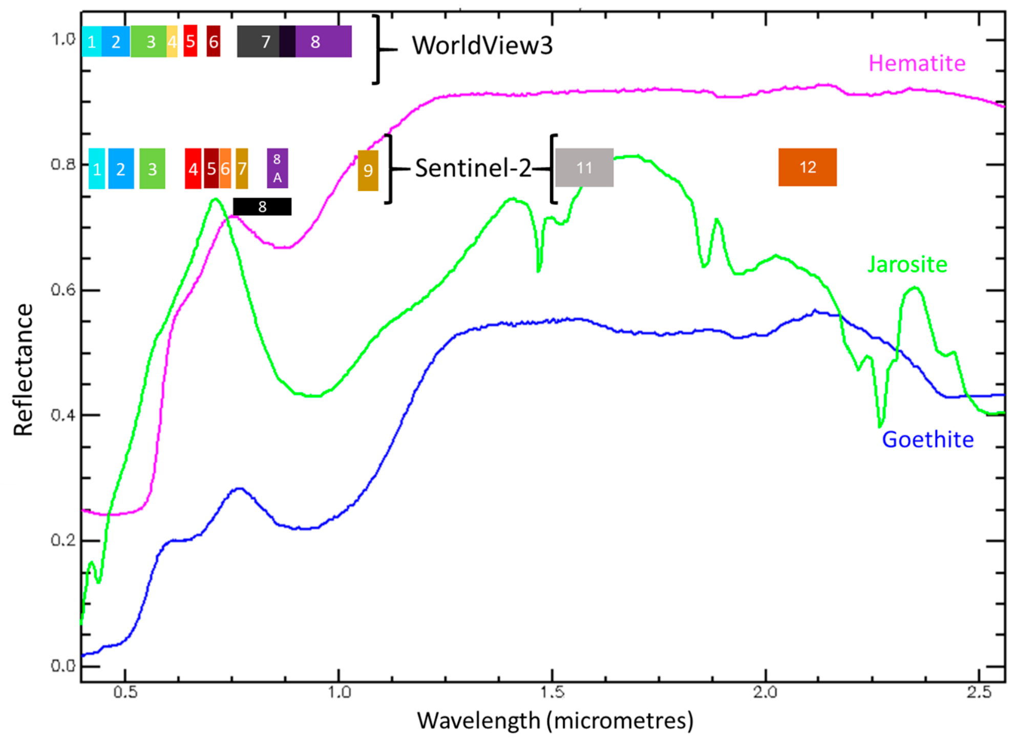
These iron-bearing minerals exhibit diagnostic spectral features in the visible–near-infrared (VNIR) region, which enables their detection using satellite remote sensing [6,7] (Figure 1). Satellite-based mapping offers a noninvasive, cost-effective, and spatially continuous approach for assessing mining-impacted landscapes, in particular over large or inaccessible areas in which conventional field-based surveys may be expensive, time-consuming, or logistically challenging. The availability of frequent satellite acquisitions enables periodic assessments, facilitating the early detection of emerging contamination hotspots and the tracking of oxidation processes over time. Such capabilities support proactive environmental risk management in both abandoned and active mining operations.

Iron-bearing minerals’ spectra are characterized by two absorption features around 450–550 nm and 800–1100 nm, as well as a reflectance maximum between 600 and 900 nm [7]. While their spectra present broad similarities among all iron minerals, the precise location of the absorbance minima and reflectance maxima allows discrimination between mineral phases depending on sensor characteristics [8,9,10].

Among freely available satellite missions, Sentinel-2 (S2) has been frequently used for mapping iron-bearing minerals in AMD-affected environments, among others [10,11,12,13]. Its multiple VNIR bands (Figure 1), including several red-edge bands, have proven effective in capturing spectral variations in secondary iron oxides and hydroxides [9,10]. However, these bands are acquired at different spatial resolutions (10, 20, and 60 m), which may limit the discrimination of minerals at local scales, as occurred, for example, in Van der Werff and Van der Meer [8], work in which the band 9, with 60 m resolution, was required to perform parabolic fitting of the absorption minimum of iron-bearing minerals for improved spectral characterization, thereby reducing spatial detail.

In contrast, the WorldView-3 (WV3) commercial satellite offers one of the best available combinations of high spatial resolution and spectral resolution, offering eight VNIR bands at 1.24 m spatial resolution uniform across all VNIR bands, and eight short-wave infrared (SWIR) bands at 3.70 m spatial resolution, also with uniform resolution across the SWIR range [9]. This configuration renders WV3 potentially feasible for mapping AMD-related materials at local scales, where mineralized distribution is heterogeneous [10]. For this reason, most mineral studies using WV3 have relied on the combined exploitation of VNIR and SWIR bands [14,15,16]. However, in some cases, WV3 data is only available in the VNIR range, either because the study cannot afford the cost of a complete WV3 image or because SWIR imagery is not present in the catalog for the study area, as occurred in this study. In addition, the relatively narrow swath width of WV3 compared with Sentinel-2 may limit its applicability for regional-scale analyses in spatially extensive and heterogeneous mining environments. Nevertheless, the use of WV3’s VNIR bands exclusively for discriminating secondary iron minerals remains less explored.

Figure 1. Iron oxide and hydroxide spectral curves and location of WV3 and S2 band wavelength range. Spectral data were obtained from [17]: Hematite GDS76, Goethite WS222, and Jarosite GDS99 K-y 200C.

Figure 1. Iron oxide and hydroxide spectral curves and location of WV3 and S2 band wavelength range. Spectral data were obtained from [17]: Hematite GDS76, Goethite WS222, and Jarosite GDS99 K-y 200C.

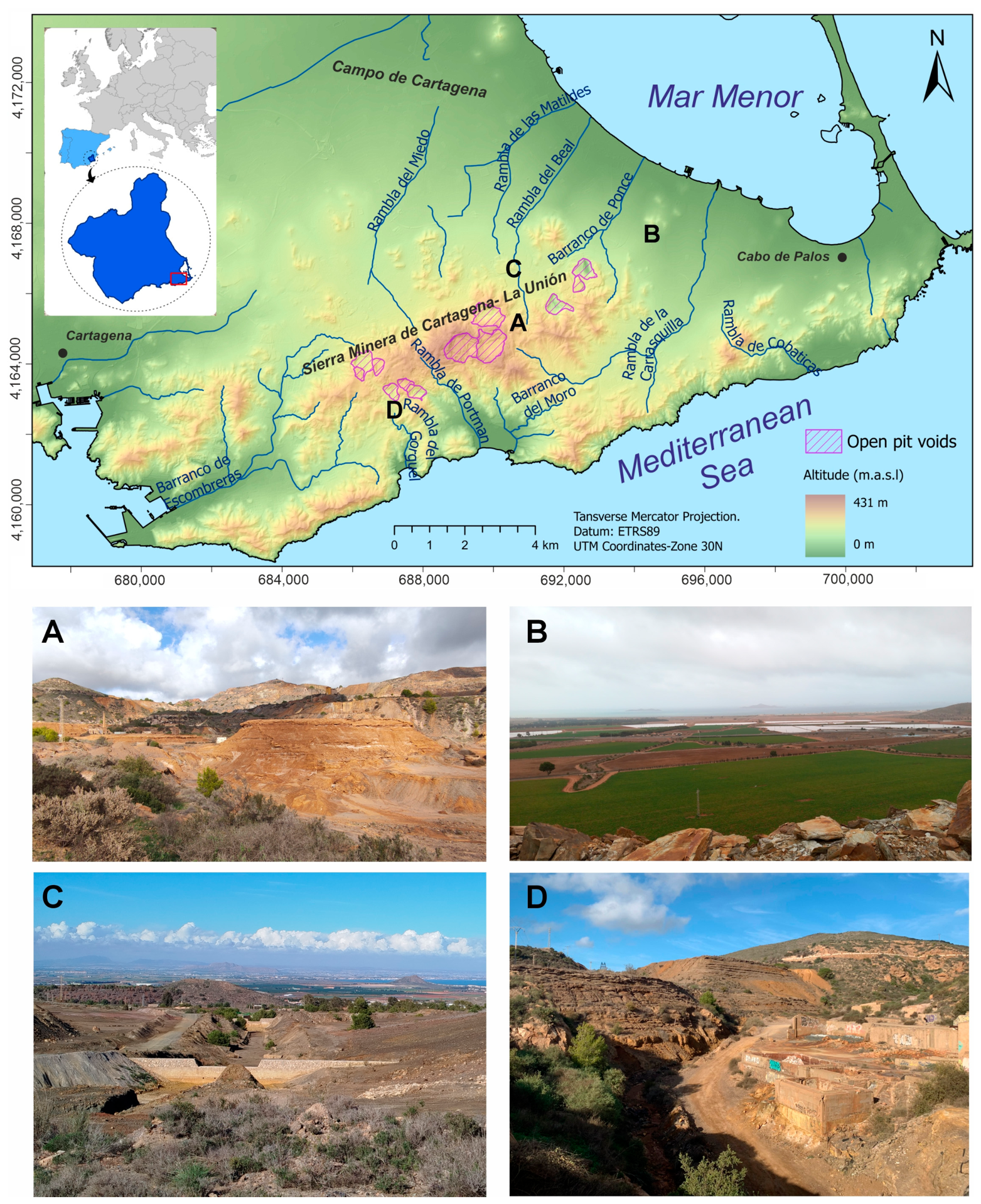
The study area is located in the Sierra Minera de Cartagena–La Unión (SE Spain), one of the most important historical mining districts on the Iberian Peninsula (Figure 2). This area has been intensively exploited for lead, zinc, and iron ores since Roman times until the late 20th century, resulting in the accumulation of large quantities of mine wastes and tailings, as well as open pits. The widespread exposure of sulfide-rich materials has led to the generation of acid mine drainage, promoting the formation of secondary iron minerals such as hematite, goethite, and jarosite across the landscape. The semi-arid Mediterranean climate, characterized by irregular but intense rainfall events, further enhances oxidation processes and episodic transport of contaminants.

In this context, a knowledge-based approach is adopted to allow a consistent and physically interpretable comparison between sensors with different spectral and spatial configurations. This approach makes it possible to detect AMD-related minerals and to evaluate what each sensor can reliably capture, considering its spatial and spectral resolution. The analysis focuses on meaningful spectral parameters, such as relative difference between bands and reflectance maxima. As these parameters are directly linked to the spectral behavior of minerals and are less dependent on scene-specific conditions, they allow for more consistent and comparable results across different satellites and acquisition conditions.

To this end, two image approaches were selected. Band ratio was chosen as it is a simple and widely used method for mineral mapping. This method exploits the relative difference between spectral bands to enhance diagnostic spectral features related to mineral composition. By normalizing one band with another, band ratio minimizes the impact of variations in illumination, topography, and albedo, while enhancing spectral differences associated with particular materials. On the other hand, a parabola fitting technique characterizes the spectral shape by fitting a second-order function to reflectance values around a spectral feature. This method is usually used to analyze absorption minima; however, in this study, it was adapted to characterize reflectance maxima. Rather than relying on discrete band values, this technique approximates the curvature and position of the feature, enabling the extraction of sub-band spectral information. This is particularly relevant in multispectral data, where broad bands do not fully resolve diagnostic features. From a physical perspective, the shape and position of reflectance peaks are controlled by the same processes that govern absorption features and therefore provide meaningful information on mineral composition.

The present study offers a comparative analysis of S2 and WV3 VNIR imagery acquired over the same AMD-affected mining area to evaluate their respective capabilities for detecting and discriminating hematite, goethite, and jarosite. To this end, two image-processing techniques are employed and compared here: band ratio and a parabola fitting technique.

2. Materials and Methods

2.1. Study Area

The study area is located in the Sierra Minera de Cartagena–La Unión, a historic mining district in southeastern Spain (Figure 2). This coastal mountain range extends for around 26 km from east to west (Figure 2A) and is bordered to the south by the Mediterranean Sea and to the north by the Campo de Cartagena (Figure 2B) basin and the Mar Menor coastal lagoon.

Mining activity in the Sierra Minera de Cartagena–La Unión started before the Roman period was established around the 3rd century BC and intensified during the 19th and 20th centuries, rendering this district one of the most important metal-producing regions in Europe. Exploitation focused on lead (Pb), zinc (Zn), and iron (Fe) from sulfide ores. Large-scale open-pit mining began in the mid-1950s, resulting in the excavation of 12 pits and the accumulation of large volumes of mining waste. Mining operations ceased in 1991; no appropriate environmental legislation existed at the time and, therefore, the subsequent lack of environmental restoration has had a lasting impact on the region’s ecological stability [18,19].

The climate of the study area is semi-arid Mediterranean, characterized by hot and dry summers and mild winters, with the mean annual precipitation ranging between 250 and 350 mm. Rainfall is highly irregular and often concentrates in short, intense events, which enhances surface runoff, erosion, and the mobilization of contaminated sediments [20]. These episodic rainfall events activate the otherwise dry ephemeral streams, locally known as ramblas (Figure 2C,D), which play a key role in the transport and redistribution of AMD-related materials across the landscape.

2.2. Satellite Imagery and Preprocessing

The S2 and WV3 images were acquired on 19 and 13 July 2020, respectively. No precipitation was recorded between the two acquisition dates; therefore, rainfall-induced mineralogical differences are not expected between the datasets. However, small variations in surface conditions, such as soil moisture, temperature, or illumination, may affect overall reflectance. In this study, these effects are considered limited, as the analysis focuses on spectral parameters such as reflectance maxima and relative difference between bands, which are mainly controlled by the intrinsic properties of the minerals and are less sensitive to changes in reflectance magnitude. Although some variations related to hydration state may occur, especially in sulphate minerals (such as jarosite), the short temporal difference between acquisitions suggests that their impact on the spectral features used for mineral discrimination is minimal.

The WV3 data consist of two mosaicked VNIR scenes with a spatial resolution of 1.24 m for the 8 bands (

Table 1. Spectral width and spatial resolution of S2 and WV3 satellites [24,25].

Sentinel-2				WorldView-3 VNIR
Name	Center (nm)	Spectral Width (nm)	Spatial Resolution (m)	Name	Center (nm)	Spectral Width (nm)	Spatial Resolution (m)
B1	443	20	60	B1	425	50	1.24
B2	490	65	10	B2	480	60	1.24
B3	560	35	10	B3	545	70	1.24
				B4	605	40	1.24
B4	665	30	10	B5	660	60	1.24
B5	705	15	20
B6	740	15	20	B6	725	40	1.24
B7	783	20	20
B8	842	115	10	B7	823.5	125	1.24
B8A	865	20	20
B9	940	20	60	B8	950	180	1.24
B11	1610	90	20
B12	2190	180	20

). The S2 dataset includes 12 spectral bands across the VNIR and SWIR ranges, with spatial resolutions of 10, 20, and 60 m, depending on the band (Table 1). Cloud cover is 10.5% for S2 and 0% for WV3. The atmospheric correction of the WV3 imagery was performed by the company Vantor (formerly Maxar) using the AComp processor [21]. The S2 data were downloaded as Level-2A surface reflectance products, atmospherically corrected by the European Space Agency using the Sen2Cor [22]. To facilitate multispectral analysis at a common spatial scale, the 20 m and 60 m bands were super-resolved to 10 m using the Sen2Res processor [23], which exploits spatial information from the higher-resolution Sentinel-2 bands to enhance the spatial detail of the lower-resolution bands while preserving their spectral characteristics.

To minimize spectral interference from vegetation and water bodies, masks were applied prior to mineral analysis. The normalized difference vegetation index (NDVI) (Equation (1)) [26] and the normalized difference water index (NDWI) (Equation (2)) [27] were calculated for both sensors. Pixels with NDVI values outside the range of 0.0 to 0.3 and NDWI values above 0.0 for S2 or above 0.04 for WV3 were masked. These thresholds were defined through an iterative evaluation by testing different values and comparing the resulting masks with the original imagery and reference areas with known vegetation and water presence. The final thresholds were selected as those that effectively excluded vegetated and water-covered areas while preserving exposed soil and mining-related materials relevant for mineral analysis. The same NDVI thresholds were obtained for both sensors, indicating a consistent response of vegetation in the VNIR region. In contrast, slight differences were observed for NDWI, likely related to differences in the spectral configuration of the NIR bands between S2 and WV3, while the green and red bands are more comparable between sensors:

$$NDVI={\displaystyle \frac{NIR-Red}{NIR+Red}}$$

(1)

$$NDWI={\displaystyle \frac{Green-NIR}{Green+NIR}}$$

(2)

where NIR corresponds to the near-infrared band,

Red corresponds to the red band,

and Green corresponds to the green band.

For S2, the NIR band corresponds to Band 8 (842 nm), the red band to Band 4 (665 nm), and the green band to Band 3 (560 nm). For WV3, the NIR band corresponds to Band 7 (823.5 nm), the red band to Band 5 (660 nm), and the green band to Band 3 (545 nm).

2.3. Iron Oxides and Hydroxides Mapping

A band ratio and a parabola fitting technique were applied, and results were compared to evaluate the ability of S2 and WV3 VNIR data to map and discriminate among iron-bearing minerals.

2.3.1. Composition Ratio of Iron Oxides and Hydroxides: Methodological Basis

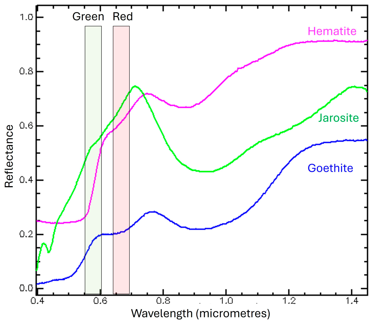
To differentiate between major iron oxides and hydroxides based on their spectral color responses, a red/green band ratio was applied. As shown in Figure 3, iron oxides and hydroxides typically show higher reflectance in the red (600–700 nm) region than in the green (500–570 nm) region [28,29]. Exploiting these differences, a ratio was proposed [28,29] to distinguish hematite, goethite, and jarosite according to their characteristic reflectance behavior (Equation (3)):

$$Iron Oxides and Hydroxides \mathrm{C}\mathrm{o}\mathrm{m}\mathrm{p}\mathrm{o}\mathrm{s}\mathrm{i}\mathrm{t}\mathrm{i}\mathrm{o}\mathrm{n} Ratio={\displaystyle \frac{Red}{Green}}$$

(3)

For S2, band 3 (560 nm) was used as the green and band 4 (665 nm) as the red. For WV3, band 3 (545 nm) and band 5 (660 nm) were employed as green and red, respectively. The resulting maps were enhanced using a 2% linear stretch and the same threshold values (0.6–4) to ensure comparability between sensors. These limits were defined based on the combined value range of both datasets, using the lowest minimum and highest maximum values of the results, allowing a consistent visualization of spectral variations across the two sensors.

The interpretation of ratio values is controlled by the relative reflectance in the green and red bands (Figure 3). High ratio values occur where reflectance in the red band is significantly higher than in the green band, which is associated with iron-rich areas dominated by minerals with strong red reflectance, such as hematite. Intermediate values are associated with minerals such as jarosite, which show a more moderate contrast between the red and green bands, with slightly higher reflectance in the red region. Lower values are associated with yellowish minerals, such as goethite, which display relatively higher reflectance in the green–yellow region and a weaker increase toward the red. However, considering the spectral overlap and frequent mineral mixing in these natural environments, these values should not be interpreted as definitive mineral identification but only as the reflection of dominant spectral trends [30,31].

2.3.2. Parabola Fitting Technique: Methodological Basis

The parabola fitting technique proposed by Van der Werff and Van der Meer [8] estimates the spectral position of diagnostic features by fitting a second-degree polynomial (parabola) to at least three spectral bands, rendering this technique suitable for multispectral imagery. Although originally developed to analyze absorption minima between 700 and 1000 nm, the method can be adapted to analyze reflectance maxima between 600 and 900 nm, which corresponds to the iron-bearing minerals’ reflectance peaks [32]. This adaptation was motivated by the limited separability of goethite and jarosite when using the absorption minima [8].

The selected wavelength range covers the diagnostic reflectance maxima of jarosite (~730 nm), goethite (~780 nm), and hematite (~860 nm) [33]. S2 offers a potentially good spectral configuration within this wavelength range, with one red band (B4), three red-edge bands (B5–B7), and two near-infrared bands (B8 and B8A). For WV3, the analysis includes four bands (B4–B7) from the same spectral interval.

The implementation of this method followed a two-step approach: (i) optimizing the band combination using laboratory spectra of hematite (samples SM-005), goethite (Samples SM-060), and jarosite (Samples SM-011) confirmed by x-ray diffraction (XRD; Section 2.4) and (ii) applying the optimized parabolic fits on a pixel-by-pixel basis to both datasets to interpolate the position of the reflectance peaks. Band optimization was performed by resampling laboratory spectra according to the spectral response of each sensor, and by evaluating different three-band combinations to identify the ones that best capture the spectral features. A second-order polynomial was fitted to each combination to reconstruct the spectral curvature, and the estimated peak position was then compared with that derived from the original, high-resolution spectra. This enabled the selection of band combinations that minimized interpolation errors associated with the discrete band configuration of multispectral data. The pixel-by-pixel implementation was carried out using a custom IDL script in the ENVI 5.6 environment (https://www.nv5geospatialsoftware.com/Products/IDL, accessed on: 1 March 2026).

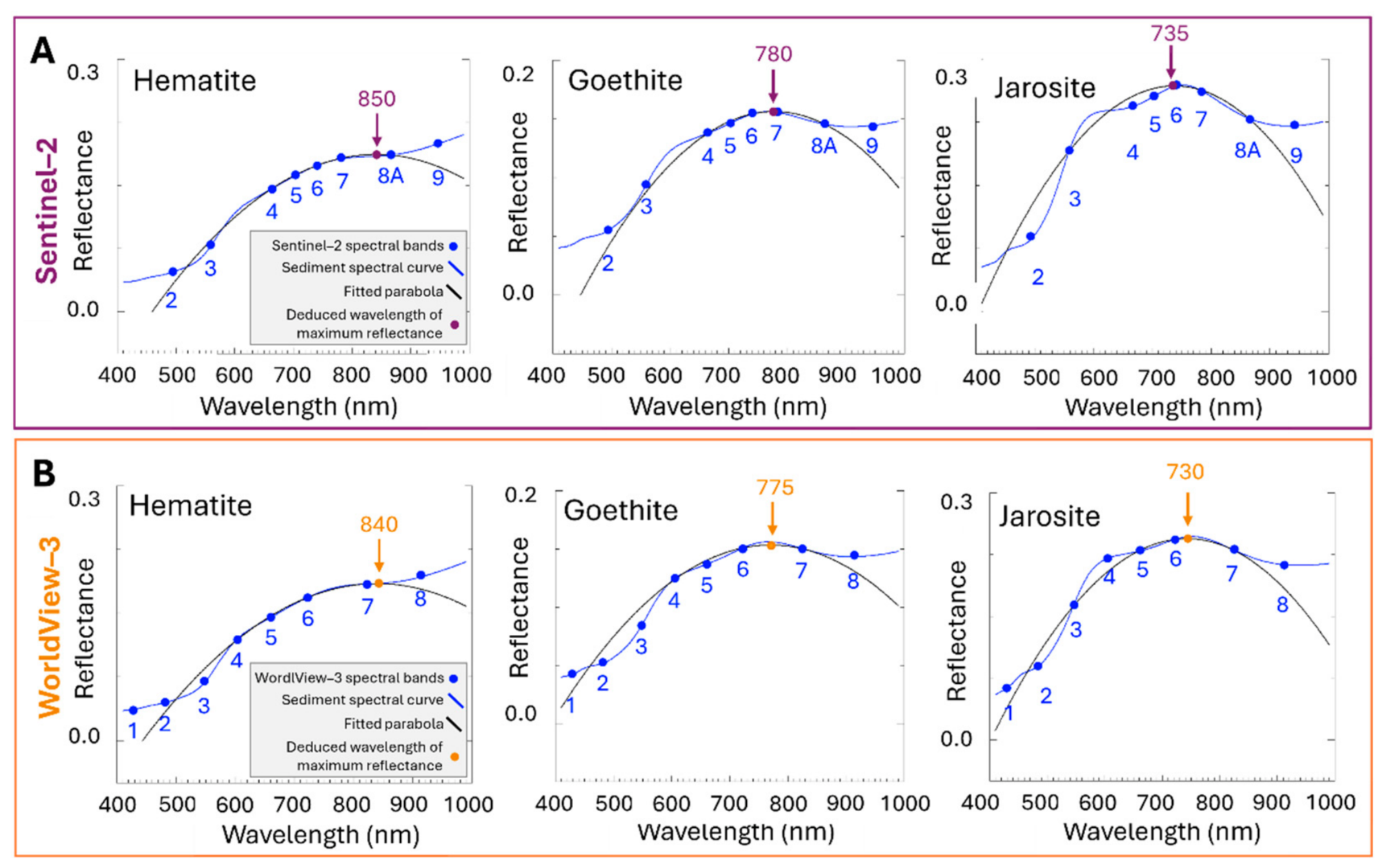
It should be noted that samples SM-005, SM-060, and SM-011, which were used to optimize the parabola fitting configuration, were also retained in the complete validation dataset (Section 2.4). However, the information used in each step was not the same. The optimization was based on ASD laboratory reflectance spectra acquired under controlled indoor conditions, whereas the validation was performed by comparing satellite-derived pixel classifications, obtained from space-borne reflectance under real atmospheric and illumination conditions, with XRD-determined mineral identities. Nevertheless, because the selection of the band combination was informed by samples that were also included in the validation set, a slight optimistic bias for these three samples cannot be completely ruled out. The best results of applying the parabola fitting technique from the S2 and WV3 band configurations to the laboratory-measured ASD spectra of the samples are shown in Figure 4. For S2 (Figure 4A), the optimal band combination is B3, B6, and B8A, while, for WV3 (Figure 4B), it was B5, B6, and B7.

The application of this technique to S2 imagery (Figure 4A) enabled the discrimination of the three minerals. The position of the reflectance maximum differed for each mineral and occurred within separate band intervals: hematite at ~850 nm between bands B7 and B8A, goethite at ~780 nm between bands B6 and B7, and jarosite at ~735 nm between bands B5 and B6. Although the polynomial fitting was based on only three bands, the interpolated parabolas align with reflectance values from at least five S2 bands. This suggests that the fitted parabolas effectively capture the spectral behavior of the minerals, confirming that the spectral configuration of S2 enables improved differentiation among hematite, goethite, and jarosite.

In the case of WV3 results (Figure 4B), reflectance maxima were identified at ~840 nm for hematite, ~775 nm for goethite, and ~730 nm for jarosite. However, due to the limited spectral resolution in this wavelength region, goethite and jarosite maxima overlapped within the band pair (B6 and B7), preventing their discrimination. In contrast, the maximum for hematite, which was located at longer wavelengths in a separate band pair (B7 and B8), could be differentiated from the goethite–jarosite group.

2.4. Validation and Field Data Collection

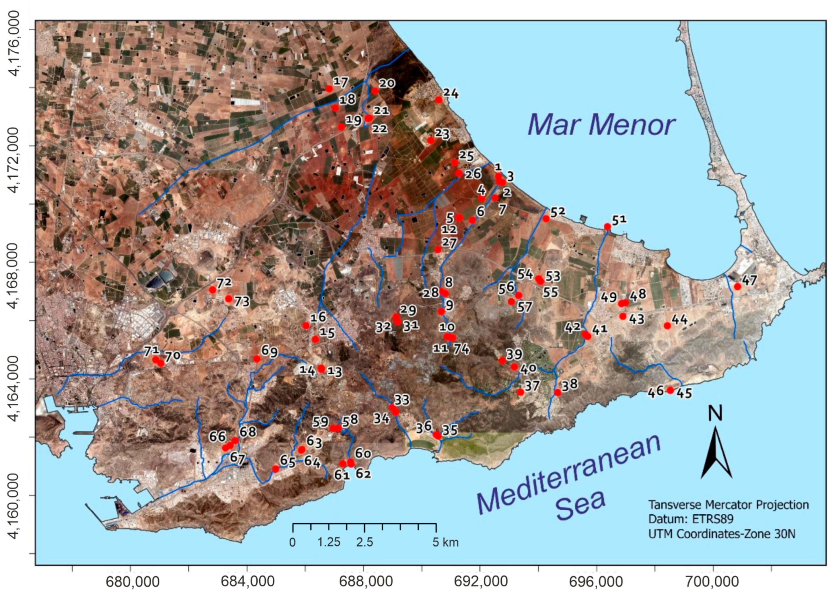
Field sampling and laboratory analysis were conducted to validate the mineral distribution maps obtained with the band ratio and the parabola fitting technique. A total of 74 sediment samples were collected from the 5 cm topsoil across several drainage basins in the Sierra Minera de Cartagena–La Unión area (Figure 5).

The sampling strategy was designed to cover both the main landforms and the mineralogical variability observed in the satellite imagery. Sample locations were first selected to cover the different geomorphic units (e.g., channel beds, alluvial deposits, mine waste, and colluvial deposits). Within each landform, samples were then distributed to capture the variability observed in the satellite imagery. This approach allowed for the capture of the variability of mineral assemblages linked to different landscape units.

Prior to laboratory analysis, all samples were air-dried. The following sample preparation for analysis varied according to the technique used. For XRD, a nondestructive technique that identifies mineral phases based on their crystal structure and characteristic diffraction patterns, the samples were homogenized into a fine powder. These analyses were performed at the Geochemistry Laboratory of the ITC, University of Twente, using a Bruker D2 PHASER diffractometer (Bruker AXS, Berlin, Germany). Mineral identification and semiquantitative analysis were conducted using DIFFRAC.EVA software (Bruker AXS, Berlin, Germany).

For validation purposes, the mineralogical composition obtained from XRD was compared with the spectral classification results extracted from the corresponding pixels in the S2 and WV3 images at each sampling location. Sampling points were selected in homogeneous areas large enough to ensure that the corresponding S2 pixel (10 m) was fully contained within a single geomorphic unit, thereby minimizing sub-pixel heterogeneity. In addition, the spatial alignment of the S2 and WV3 images was verified. Therefore, no additional buffering or spatial averaging was applied.

In addition to validation, XRD results were used to select three representative samples each dominated by hematite (SM-005), goethite (SM-060), and jarosite (SM-011) for laboratory spectral characterization. These samples were also included in the complete validation dataset. Spectral measurements were then performed using the original samples. The reflectance spectra were acquired at the University of León (QGEO research group) using an ASD FieldSpec 4 Standard-Res spectroradiometer (Analytical Spectral Devices, Inc., Boulder, CO, USA) (https://www.malvernpanalytical.com/en/products/product-range/asd-range/fieldspec-range/fieldspec4-hi-res-high-resolution-spectroradiometer, accessed on 1 March 2026) over the VNIR–SWIR range (350–2500 nm), with spectral resolutions of 3 nm in the 350–1000 region and 5 nm in the 1000–2500 nm region. Three different measurements were taken in each sample using a contact probe, and the averaged spectrum was used as the representative reflectance signature of each iron mineral.

2.5. Cross-Sensor Comparison

To quantitatively evaluate the agreement between S2 and WV3, a pixel-based cross-sensor comparison was performed using discrete classifications derived from both the composition band ratio and the parabola fitting technique.

• Composition band ratio classification

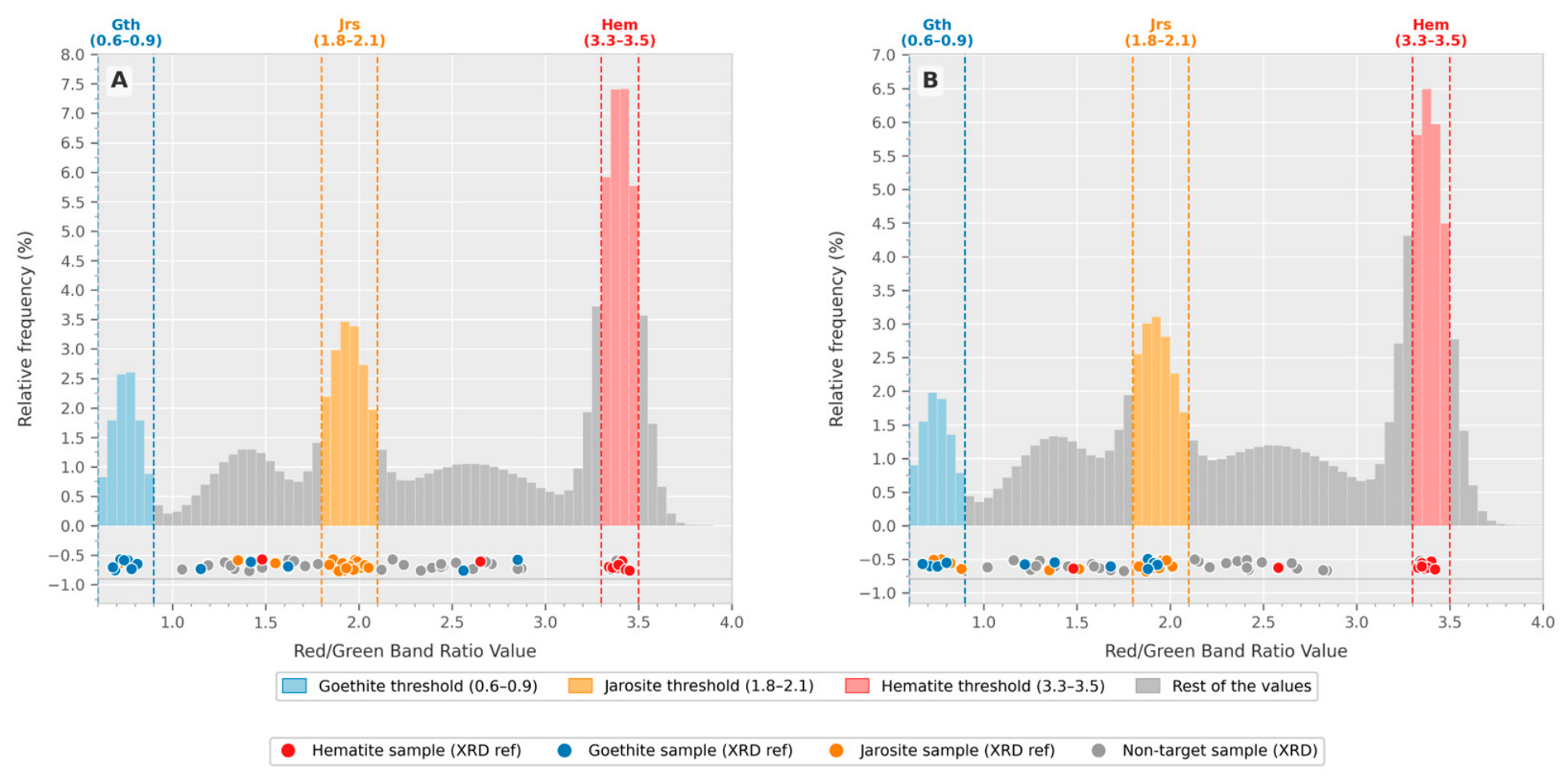
Continuous outputs were converted into discrete mineral maps. For the composition band ratio, the threshold ranges were derived following the methodology proposed by Cudahy [31]. The thresholds were defined empirically based on the distribution of ratio values and supported by XRD-identified mineral assemblages. The resulting ranges were applied consistently to the resulting maps from both sensors: 0.6–0.9 for goethite, 1.8–2.1 for jarosite, and 3.3–3.5 for hematite. Pixels falling outside these intervals were classified as no mineral.

The same threshold ranges were applied to S2 and WV3 to ensure a consistent comparison between classifications. Although both sensors have different spectral response functions and bandwidths, the bands used in the ratio are centered at similar wavelengths in the green and red regions (Table 1), resulting in comparable spectral responses. Moreover, the thresholds were not defined from theoretical sensor-specific values, but empirically from the ratio value distribution and supported by XRD results. Applying a common set of thresholds therefore allowed differences between the resulting maps to be interpreted mainly in relation to sensor characteristics rather than differences in classification criteria. In this context, the thresholds should be interpreted as operational limits established for consistent classification and cross-sensor comparison.

To illustrate the position of the selected threshold ranges within the ratio value distribution of the study area, and the location of the 74 validation samples within that distribution, Figure 6 shows the ratio histograms for both sensors alongside the sample positions colored by the XRD reference class. In this context, the thresholds should be interpreted as operational limits established to enable consistent classification and comparison between sensors, rather than as definitive mineralogical boundaries, given the spectral overlap and the presence of mixed pixels.

• Threshold sensitivity analysis

To evaluate the robustness of the selected thresholds, a sensitivity analysis was carried out by symmetrically varying the width of each threshold by ±0.05 and ±0.10 ratio units while maintaining the original threshold center. Classification performance under each scenario was evaluated using the 74 validation samples (

Table 2. Sensitivity analysis of threshold selection for the S2 composition band ratio. The center of each threshold was kept fixed while the width was varied symmetrically by ±0.05 and ±0.10 ratio units on each side. For the −0.10 scenario, the hematite threshold is not applicable (—).

Width Change	Threshold Ranges (Gth/Jrs/Hem)	Correctly Classified (n/74)	Target Minerals Not Detected (n/41)	Non-Target False Positives (n/33)	Target Mineral Accuracy (n/41)
−0.10 (narrower)	0.70–0.80 1.90–2.00 —	46 (62.2%)	26 (63.4%)	0 (0.0%)	13 (31.7%)
−0.05 (narrower)	0.65–0.85 1.85–2.05 3.35–3.45	58 (78.4%)	12 (29.3%)	2 (6.1%)	27 (65.9%)
0(original)	0.60–0.90 1.80–2.10 3.30–3.50	61 (82.4%)	9 (22.0%)	2 (6.1%)	30 (73.2%)
+0.05 (wider)	0.55–0.95 1.75–2.15 3.25–3.55	57 (77.0%)	9 (22.0%)	6 (18.2%)	30 (73.2%)
+0.10 (wider)	0.50–1.00 1.70–2.20 3.20–3.60	54 (73.0%)	9 (22.0%)	9 (27.3%)	30 (73.2%)

and

Table 3. Sensitivity analysis of threshold selection for the WV3 composition band ratio. The center of each threshold was kept fixed while the width was varied symmetrically by ±0.05 and ±0.10 ratio units on each side. For the −0.10 scenario, the hematite threshold is not applicable (—).

Width Change	Threshold Ranges (Gth/Jrs/Hem)	Correctly Classified (n/74)	Target Minerals Not Detected (n/41)	Non-Target False Positives (n/33)	Target Mineral Accuracy (n/41)
−0.10 (narrower)	0.70–0.80 1.90–2.00 —	45 (60.8%)	24 (58.5%)	0 (0.0%)	12 (29.3%)
−0.05 (narrower)	0.65–0.85 1.85–2.05 3.35–3.45	54 (73.0%)	10 (24.4%)	1 (3.0%)	22 (53.7%)
0(original)	0.60–0.90 1.80–2.10 3.30–3.50	55 (74.3%)	7 (17.1%)	2 (6.1%)	24 (58.5%)
+0.05 (wider)	0.55–0.95 1.75–2.15 3.25–3.55	51 (68.9%)	7 (17.1%)	6 (18.2%)	24 (58.5%)
+0.10 (wider)	0.50–1.00 1.70–2.20 3.20–3.60	49 (66.2%)	7 (17.1%)	8 (24.2%)	24 (58.5%)

).

In the −0.10 scenario, the hematite threshold collapsed to a single value (3.40–3.40) and was therefore omitted; consequently, all hematite samples were considered unclassified.

The sensitivity analysis revealed two consistent trends for both sensors. Narrower thresholds substantially reduced target-mineral accuracy because more target samples fell outside the classification ranges and remained unclassified. Conversely, wider thresholds did not improve target-mineral accuracy but progressively increased the number of false positives by assigning additional non-target samples to mineral classes. These results indicate that the original threshold ranges provide the best compromise between mineral detection and false-positive control for this dataset, supporting their use as operational thresholds rather than fixed mineralogical boundaries.

• Parabola fitting classification

For the parabola fitting technique, the interpolated wavelength of maximum reflectance was used to classify the maps (Figure 4). Pixels were assigned to a mineral class when the estimated maximum fell within ±5 nm of the laboratory-derived reference wavelength. The ±5 nm window was used as an operational tolerance to account for minor uncertainty in the interpolation of the reflectance maximum from multispectral bands and small spectral shifts between laboratory and image-derived spectra.

• Pixel-based comparison

To assess the influence of spatial resolution on classification consistency, S2 classifications were resampled to the ~1.2 m spatial resolution of WV3 using a nearest neighbor approach, preserving the original spectral values. The resampling was performed to match the spatial resolution and grid of WV3, ensuring proper alignment between both datasets. This step does not increase spatial detail, and the resampled S2 pixels do not represent independent 1.24 m observations; each resampled pixel retains the spectral information of the original 10 m S2 pixel and is spatially replicated across the WV3 grid solely to enable pixel-by-pixel alignment. Consequently, the reported pixel counts reflect the WV3-resolution grid and should not be interpreted as implying that S2 provides 1.24 m spatial information. This resampling step enables the evaluation of whether the higher spatial resolution of WV3 provides additional discriminatory detail in small-scale and heterogeneous areas, such as narrow drainage channels.

All comparisons were restricted to the coincident area between both datasets, corresponding to the overlapping extent of the S2 and WV3 images, as S2 covers a larger area than WV3. This restriction is necessary because WV3 has a much narrower image swath width, approximately 13 km at nadir, compared with the 290 km swath width of Sentinel-2. Cross-tabulation matrices were generated by intersecting the classified maps on a pixel-by-pixel basis. These matrices quantify agreement or disagreement between sensors for each mineral class. Additionally, spatial agreement maps were produced to visualize the spatial distribution of coincident and not-matched classifications and to identify those areas in which the spatial resolution influences mineral discrimination.

3. Results

3.1. Composition Ratio of Iron Oxides and Hydroxides: Spatial Results

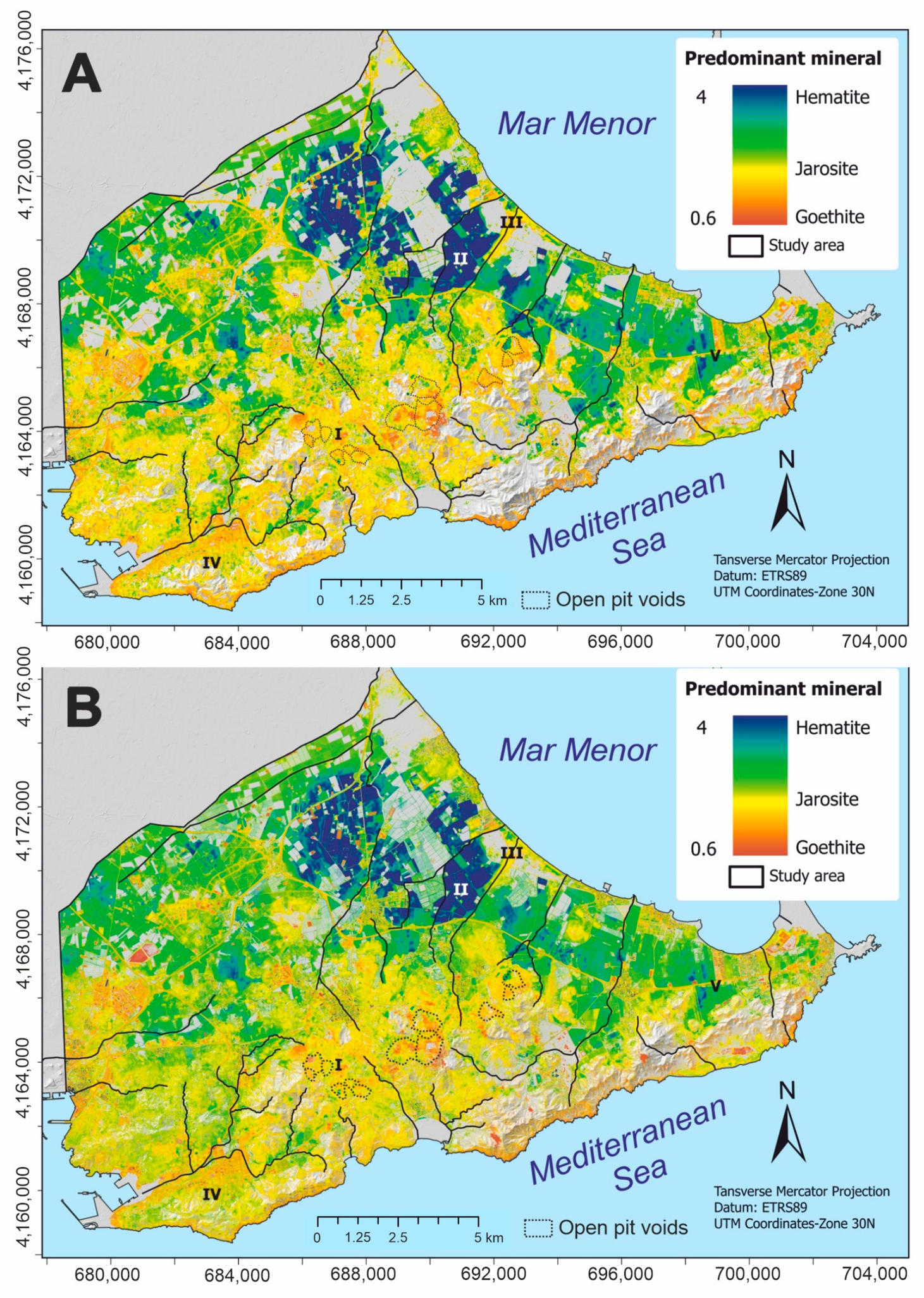
The spatial distribution and composition of iron oxides and hydroxides are shown in Figure 7.

The compositional maps (Figure 7) show hematite to be the most widespread mineral in the areas draining into the Mar Menor (Figure 7A,B, Zone II). Goethite and jarosite concentrate mainly near drainage channels, in headwater sections, and in areas draining into the Mediterranean Sea (Figure 7A,B, Zone I). However, a large proportion of areas mapped as jarosite (with intermediate values) is observed. This relates to how band ratios work, where all pixels are assigned a continuous value. As a result, many pixels with intermediate responses—although not strictly within the defined jarosite thresholds—appear with similar values, giving the impression of overrepresentation. This highlights the importance of carefully defining and applying classification thresholds. Results from both sensors show similar spatial patterns of mineral distribution (Figure 7A,B).

3.2. Parabola Fitting Technique: Spatial Results

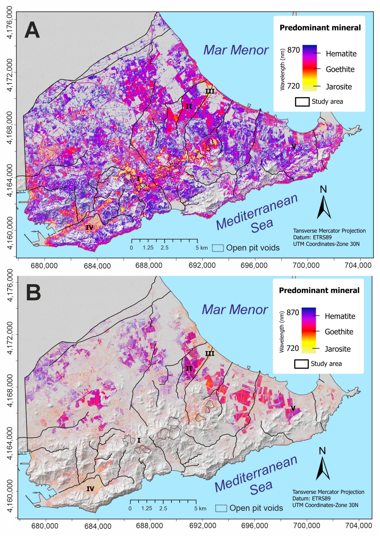
Mineral distribution maps were generated based on the constructed parabolas (Figure 4). The classification results show a difference between the two sensors in the surface classification. S2 (Figure 8A) classified a larger area than that classified by WV3 (Figure 8B). While WV3 classified pixels mainly from the downstream area of the Campo de Cartagena (Figure 8B), S2 also classified the headwater section and the basins draining towards the Mediterranean Sea (Figure 8A).

The larger number of unclassified pixels in the WV3 parabola fitting result should therefore be interpreted as part of the method performance, rather than only as missing spatial coverage. These unclassified pixels indicate areas where the estimated reflectance maximum did not meet the classification criteria for hematite, goethite, or jarosite, reflecting the limited ability of WV3 VNIR bands to resolve some diagnostic spectral differences.

Both sensors indicate hematite as the predominant mineral across the Campo de Cartagena (Figure 8A,B, Zone II). The S2 map (Figure 8A, Zone I) shows goethite and jarosite in the headwater section, corresponding to the Sierra Minera de Cartagena–La Unión, where the majority of historical mine waste deposits are concentrated. Also, these can be observed adjacent to the ramblas with a clear presence in the central one in the study area (Rambla del Beal; (Figure 8, Zone III).

In the southwestern sector (Figure 8, Zone IV), S2 also indicates the presence of jarosite and goethite. However, said presence corresponds to an industrial zone rather than natural soils or sediments. The spectral response is likely influenced by iron oxide-based coatings and weathered metallic surfaces, which produce reflectance patterns in the visible range similar to those of natural iron oxides and hydroxides.

3.3. Validation

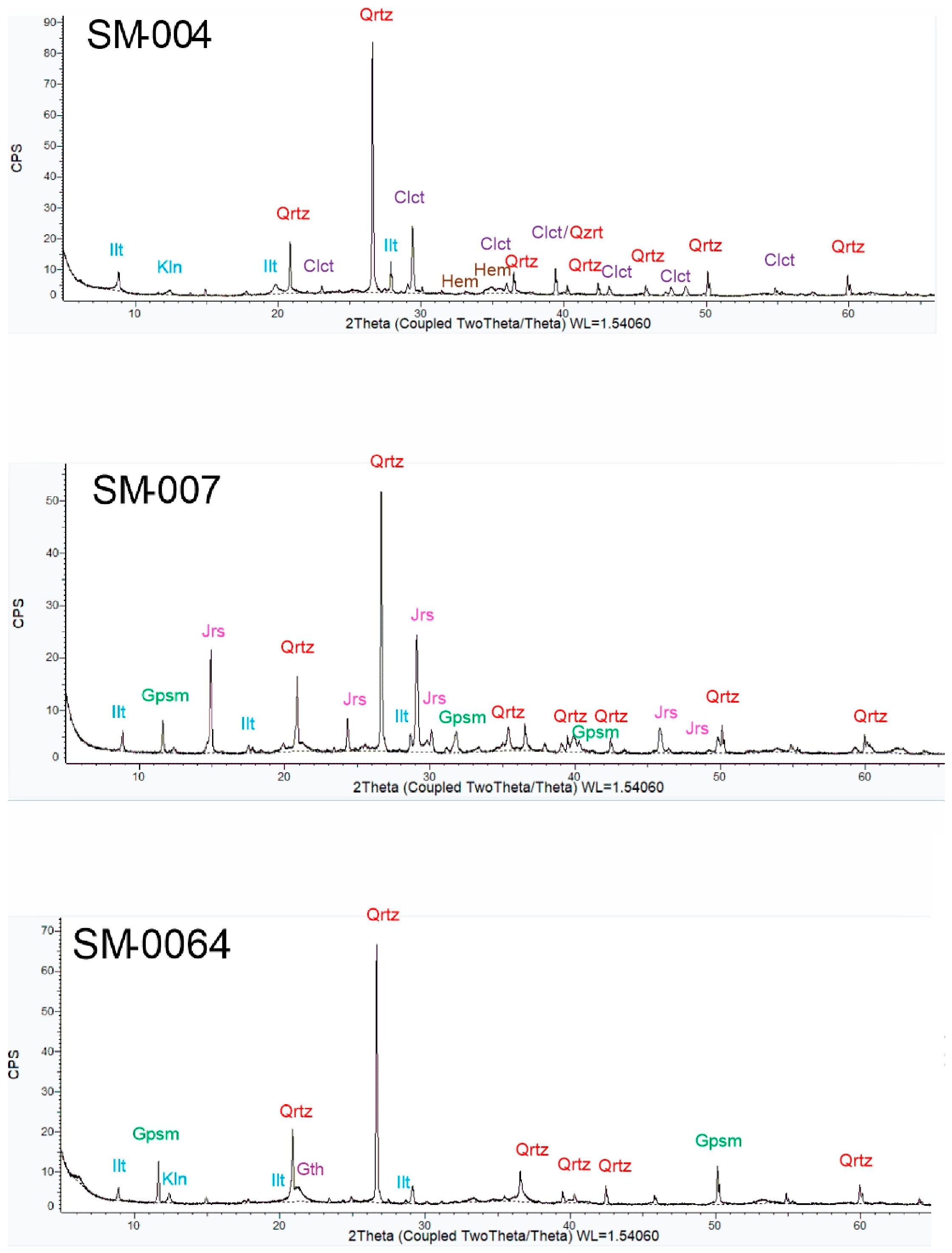
The spectral classification results were validated using XRD analysis for 74 samples. The detailed sample-level comparison is presented in

Table 4. Location of samples analyzed by XRD, with the corresponding S2 and WV3 results: composition band ratio and parabola fitting technique. Minerals identified by XRD are listed in order of decreasing abundance. Green cells indicate agreement between the spectral classification and XRD results, whereas red cells indicate disagreement. Empty cells indicate that the spectral method was applied but no target mineral was identified. X indicates samples that were not classified by the spectral method.

Sample ID	Latitude (UTM)	Longitude (UTM)	XRD a	Composition Band Ratio b		Parabola Fitting Technique b
				S2	WV3	S2	WV3
SM-001	692,622	4,170,952	Qrtz, Ha, Kln, Gpsm, Jrs, (Gth)	Jrs	Jrs	X	Jrs
SM-002	692,653	4,170,791	Qrtz, Gpsm, Jrs, (Gth)	Gth	Jrs	Gth	Jrs
SM-003	692,770	4,170,765	Qrtz, Ha, Ilt, Kln, Jrs, (Gth)	Jrs	Jrs	X	Jrs
SM-004	692,063	4,170,197	Qrtz, Clct, Kln, (Ilt), (Hem)	Hem	Hem	Hem	Hem
SM-005	691,311	4,169,486	Qrtz, Clct, Kln, (Ilt), (Hem)	Hem	Hem	Hem	Hem
SM-006	691,749	4,169,460	Qrtz, Gpsm, Jrs, Gth, (Ilt)	Jrs	Gth	Jrs	Jrs
SM-007	692,499	4,170,225	Qrtz, Gpsm, Jrs, (Ilt)	Jrs	Jrs	X	Jrs
SM-008	690,642	4,167,014	Kln, Qrtz, Jrs, Gpsm, (Ilt)	Jrs	Gth	Jrs	Gth
SM-009	690,671	4,166,309	Qrtz, Dlmt, Clct, Gpsm, Jrs, (Ilt)	Jrs	Jrs	Jrs	Jrs
SM-010	690,862	4,165,445	Qrtz, Gpsm, Kln, Gth, Jrs, (Ilt)	X	Jrs	X	X
SM-011	691,053	4,165,406	Qrtz, Jrs, (Gpsm), (Ilt)	Jrs	Jrs	Jrs	Jrs
SM-012	691,280	4,169,469	Qrtz, Clct, Kln, (Ilt), (Hem)	Hem	Hem	X	Hem
SM-013	686,554	4,164,326	Kln, Qrtz, Gpsm, Gth, Fhy, (Jrs), (Ilt)	Gth	Jrs	Gth	X
SM-014	686,548	4,164,367	Kln, Qrtz, Gpsm, Fhy, (Jrs), (Pyrm), (Ilt)	Jrs	Jrs	X	Jrs
SM-015	686,348	4,165,358	Kln, Gpsm, Ilt, Qrtz, Chl, Gth	X	Gth	Gth	X
SM-016	686,034	4,165,850	Qrtz, Clct, Kln, Ilt, (Al)
SM-017	686,821	4,173,970	Qrtz, Clct, Kln, Ilt
SM-018	687,022	4,173,314	Qrtz, Clct, Kln, Ilt
SM-019	687,234	4,172,652	Qrtz, Clct, Ilt, (Kln), (Hem)	Hem	Hem	Hem	Hem
SM-020	688,393	4,173,901	Qrtz, Clct, Ilt, (Kln)
SM-021	688,208	4,172,949	Qrtz, Clct, Ilt, (Kln), (Hem)	Hem	Hem	Hem	Hem
SM-022	688,144	4,172,943	Qrtz, Clct, Ilt, (Kln)
SM-023	690,300	4,172,194	Qrtz, Clct, Ilt, (Kln), (Hem)	Hem	Hem	Hem	X
SM-024	690,578	4,173,576	Qrtz, Clct, Ilt, (Kln)
SM-025	691,136	4,171,422	Qrtz, Clct, Ilt, (Kln)	Hem	Hem
SM-026	691,279	4,171,054	Qrtz, Clct, Ilt, (Kln)			Hem
SM-027	690,547	4,168,433	Qrtz, Clct, Kln, Ilt	Hem	Hem
SM-028	690,801	4,166,932	Qrtz, Kln, Ilt, (Gth)	X	X	Gth	X
SM-029	689,115	4,166,129	Gpsm, Jrs, Gth, Qrtz	Jrs	X	Jrs	Gth
SM-030	689,114	4,166,154	Gpsm, Jrs, Gth, Qrtz, (Clct)	Jrs	X	Jrs	X
SM-031	689,167	4,165,962	Kln, Gpsm, Jrs, Gth, (Hem), (Qrtz)	Jrs	Gth	X	X
SM-032	689,157	4,165,983	Qrtz, Kln, Ilt, (Gth)	Gth	Gth	Gth	X
SM-033	689,100	4,162,862	Qrtz, Gpsm, Jrs, Gth, (Ilt)	Jrs	Jrs	Jrs	Jrs
SM-034	688,985	4,163,013	Qrtz, Jrs, Gth, (Ilt)	Jrs	Jrs	Jrs	Gth
SM-035	690,555	4,162,030	Ilt, Jrs, Kln, Qrtz, Gth	X	Gth	X	Gth
SM-036	690,497	4,162,084	Gpsm, Qrtz, Ilt, Colt, Jrs, Kln	Jrs	Jrs	Jrs	Jrs
SM-037	693,387	4,163,543	Qrtz, Clct, Kln, Ilt, (Hem)	X	Hem	Hem	Hem
SM-038	694,656	4,163,533	Qrtz, Clct, Kln, Ilt			Hem
SM-039	692,759	4,164,623	Qrtz, Gpsm, Kln, Dol, (Gth), (Ilt)	Gth	X	Gth	X
SM-040	693,171	4,164,411	Qrtz, Clct, Kln, Ilt
SM-041	695,693	4,165,457	Qrtz, Clct, Kln, Ilt
SM-042	695,601	4,165,532	Qrtz, Clct, Kln, Ilt
SM-043	696,901	4,166,148	Qrtz, Clct, Kln, Ilt
SM-044	698,423	4,165,822	Qrtz, Clct, Kln, Ilt
SM-045	698,529	4,163,601	Clct, Qrtz, Ara, (Ilt)
SM-046	698,524	4,163,605	Qrtz, Clct, Ara, Dol, Gth, Kln	Gth	X	X	X
SM-047	700,836	4,167,164	Qrtz, Kln, Clct, (Ilt)
SM-048	696,988	4,166,618	Qrtz, Clct, Kln, Ilt
SM-049	696,847	4,166,584	Qrtz, Clct, Kln, (Ilt)
SM-050	696,367	4,169,213	Gpsm, Ilt, Qrtz, Ha, Jrs	X	Jrs	Jrs	X
SM-051	696,369	4,169,218	Qrtz, Clct, Kln, Gpsm, (Ilt)
SM-052	694,262	4,169,509	Qrtz, Clct, Kln, Ilt
SM-053	694,072	4,167,346	Qrtz, Clct, Kln, (Ilt)
SM-054	694,005	4,167,439	Qrtz, Clct, Kln, (Ilt), (Hem)	Hem	X	Hem	X
SM-055	694,030	4,167,398	Qrtz, Clct, Ilt, (Kln)
SM-056	693,324	4,166,865	Qrtz, Clct, Kln, Ilt
SM-057	693,072	4,166,649	Chlorite, Ilt, Qrtz, Gpsm, Jrs, Dol	Jrs	Jrs	Jrs	X
SM-058	687,123	4,162,307	Gpsm, Clct, Qrtz, Kln, Gth, (Ilt)	Gth	Jrs	Gth	Gth
SM-059	686,948	4,162,305	Gpsm, Qrtz, Kln, Jrs, Gth, (Clct), (Ilt)	Gth	Gth	Jrs	X
SM-060	687,554	4,161,144	Gpsm, Qrtz, Gth, (Ilt)	Gth	Gth	Gth	Gth
SM-061	687,287	4,161,083	Gpsm, Qrtz, Jrs, (Ilt)	Jrs	Jrs	Jrs	Jrs
SM-062	687,575	4,161,071	Kln, Sid, Ilt, Qrtz, Dol, Ma, Pyr, Gth, Sph, Hem	X	Gth	Gth	Gth
SM-063	685,888	4,161,572	Chl, Ilt, Gpsm, Sid, (Hem), (Jrs), (Qrzt)	X	X	X	X
SM-064	685,867	4,161,548	Qrtz, Ilt, Gpsm, Kln, Gth	Gth	Jrs	Gth	Jrs
SM-065	684,979	4,160,908	Qrtz, Clct, Kln, (Ilt)
SM-066	683,410	4,161,714	Qrtz, Clct, Kln, (Ilt)
SM-067	683,238	4,161,640	Qrtz, Clct, Kln, (Ilt)
SM-068	683,593	4,161,880	Qrtz, Clct, Kln, (Ilt)
SM-069	684,342	4,164,688	Qrtz, Clct, Kln, (Ilt)
SM-070	681,045	4,164,535	Qrtz, Clct, Kln, (Ilt)
SM-071	680,868	4,164,654	Qrtz, Clct, Kln, (Ilt)
SM-072	682,822	4,167,063	Qrtz, Clct, Kln, (Ilt)
SM-073	683,370	4,166,746	Qrtz, Clct, Kln, (Ilt)
SM-074	690,968	4,165,439	Qrtz, (Gth), (Gpsm), (Ilt), (Jrs)	X	Jrs	X	Jrs

Al: alunite, Ara: aragonite, Chl: chlorite, Clct: calcite, Dol: dolomite, Fhy: ferrihydrite, Gpsm: gypsum, Gth: goethite, Ha: halite, Hem: hematite, Ilt: illite, Jrs: jarosite, Kln: kaolinite, Mag: magnetite, Pyr: pyrite, Pyrm: pyromorphite, Qrtz: quartz, Sid: siderite, and Sph: sphalerite. ^a XRD data: major phase (>20% by weight) in bold, minor phase (5–20% by weight) as plain text; () indicates trace phase (<5% by weight). ^b plain text indicates only presence of the mineral. Empty cells indicate that the spectral method was applied but no target mineral was identified. X indicates that the sample was not classified by the spectral method.

. The mineralogical composition determined by XRD and the classifications obtained from S2 and WV3 using both the composition band ratio and the parabola fitting technique are presented in the Table. Figure 9 shows representative diffractograms for three samples (one dominated by hematite, one by goethite, and one by jarosite).

In Table 4, minerals identified by XRD are reported in order of decreasing abundance. For validation purposes, only the iron-bearing minerals targeted in this study (hematite, goethite, and jarosite) were considered. The reference mineral for each sample was defined as the most abundant among these iron minerals identified by XRD. Consequently, a classification was considered correct only when the spectrally identified mineral matched this reference mineral.

Table 5. Summary of spectral classification outcomes for the 74 analyzed samples.

	Classification Method
	Composition Band Ratio		Parabola Fitting Technique
	S2	WV3	S2	WV3
Overall agreement including non-target samples	61 (82.4%)	55 (74.3%)	60 (81.1%)	53 (71.6%)
Disagreement	4 (5.4%)	12 (16.2%)	3 (4.1%)	6 (8.1%)
Not classified	9 (12.2%)	7 (9.5%)	11 (14.9%)	15 (20.3%)

“Overall agreement including non-target samples” indicates agreement between the spectral classification and XRD results, including both correct target-mineral classifications and correct non-classification of non-target samples. “Disagreement” refers to cases where the mineral assigned by the spectral method differs from the reference mineral identified by XRD. “Not classified” indicates samples for which a target mineral was identified by XRD but no mineral class was assigned by the spectral method. Values in parentheses represent percentages relative to the total number of samples.

summarizes the validation results for the 74 analyzed samples, showing the number of samples in agreement with XRD, in disagreement with XRD, and not classified by each spectral method and sensor. Agreement includes both samples correctly assigned to one of the target minerals and samples correctly identified as non-targets, when no hematite, goethite, or jarosite was reported as the reference mineral by XRD. Therefore, the percentages reported in Table 5 represent overall agreement including non-target samples.

A high level of consistency was observed when comparing XRD and S2 composition band ratio, with most of the hematite, goethite, and jarosite samples being correctly identified. Using this method, 61 samples were correctly classified, four were misclassified, and nine unclassified. Most of the misclassifications were associated with samples containing mixed mineral assemblages. In contrast, the WV3 composition band ratio resulted in lower consistency, with 55 samples correctly classified, 12 misclassified, and seven unclassified. Misclassification in this case was especially evident in jarosite–goethite mixtures and in samples with low iron content. Also, the WV3 composition band ratio occasionally assigned iron minerals to samples in which none were confirmed by XRD.

The parabola fitting technique showed a good correspondence with XRD when applied to the S2 image: 60 samples were correctly classified, three failed to be detected, and 11 samples were unclassified. In contrast, the application of this technique to WV3 data resulted in the lowest level of consistency, with 53 correctly classified samples, six misclassified samples, and 15 unclassified samples. Misclassifications were mainly due to confusion between jarosite and goethite.

The confusion matrices in

Table 6. The Sentinel-2 composition band ratio confusion matrix combines absolute values and row-normalized percentages (in parentheses). The percentages are calculated relative to each ground-truth class (row-wise).

		Predicted
		Hematite	Goethite	Jarosite	Not Classified
Truth	Hematite (n = 9)	7 (77.8%)	0 (0.0%)	0 (0.0%)	2 (22.2%)
	Goethite (n = 12)	0 (0.0%)	7 (58.3%)	0 (0.0%)	5 (41.7%)
	Jarosite (n = 20)	0 (0.0%)	2 (10.0%)	16 (80.0%)	2 (10.0%)
	Not classified (n = 33)	2 (6.1%)	0 (0.0%)	0 (0.0%)	31 (93.9%)

,

Table 7. The WorldView-3 composition band ratio confusion matrix combines absolute values and row-normalized percentages (in parentheses). The percentages are calculated relative to each ground-truth class (row-wise).

		Predicted
		Hematite	Goethite	Jarosite	Not Classified
Truth	Hematite (n = 9)	7 (77.8%)	0 (0.0%)	0 (0.0%)	2 (22.2%)
	Goethite (n = 12)	0 (0.0%)	4 (33.3%)	5 (41.7%)	3 (25.0%)
	Jarosite (n = 20)	0 (0.0%)	5 (25.0%)	13 (65.0%)	2 (10.0%)
	Not classified (n = 33)	2 (6.1%)	0 (0.0%)	0 (0.0%)	31 (93.9%)

,

Table 8. The Sentinel-2 parabola fitting technique confusion matrix combines absolute values and row-normalized percentages (in parentheses). The percentages are calculated relative to each ground-truth class (row-wise).

		Predicted
		Hematite	Goethite	Jarosite	Not Classified
Truth	Hematite (n = 9)	7 (77.8%)	0 (0.0%)	0 (0.0%)	2 (22.2%)
	Goethite (n = 12)	0 (0.0%)	9 (75.0%)	0 (0.0%)	3 (25.0%)
	Jarosite (n = 20)	0 (0.0%)	1 (5.0%)	13 (65.0%)	6 (30.0%)
	Not classified (n = 33)	2 (6.1%)	0 (0.0%)	0 (0.0%)	31 (93.9%)

and

Table 9. The WorldView-3 parabola fitting technique confusion matrix combines absolute values and row-normalized percentages (in parentheses). The percentages are calculated relative to each ground-truth class (row-wise).

		Predicted
		Hematite	Goethite	Jarosite	Not Classified
Truth	Hematite (n = 9)	6 (66.7%)	0 (0.0%)	0 (0.0%)	3 (33.3%)
	Goethite (n = 12)	0 (0.0%)	3 (25.0%)	2 (16.7%)	7 (58.3%)
	Jarosite (n = 20)	0 (0.0%)	4 (20.0%)	11 (55.0%)	5 (25.0%)
	Not classified (n = 33)	0 (0.0%)	0 (0.0%)	0 (0.0%)	33 (100%)

offer a comparative evaluation of classification performance applied to S2 (Table 6 and Table 7) and WV3 (Table 8 and Table 9) data. Overall, hematite is consistently well detected by all methods, with accuracies between 66.7% and 77.8%. The “Not classified” category also shows very good performance (>93%), indicating that false positives are limited. Jarosite generally exhibits moderate-to-high accuracy, particularly with the composition band ratio methods (80.0% for S2 and 65.0% for WV3). In contrast, goethite is the most challenging mineral to discriminate and shows the greatest variability between methods (25.0–75.0%). The best results for goethite are obtained with the Sentinel-2 parabola fitting technique (75.0%), whereas in the other approaches it is more frequently confused with jarosite or remains unclassified. Notably, the Sentinel-2 parabola fitting technique improves results to 75.0%, compared to other approaches where confusion with jarosite or unclassified pixels is more prevalent.

Table 10. Per-class precision, recall, and F1-score for the 41 target-mineral samples (hematite n = 9, goethite n = 12, and jarosite n = 20) across all four classification methods, together with overall target-mineral accuracy.

		Classification Method
		Composition Band Ratio		Parabola Fitting Technique
		S2	WV3	S2	WV3
Hematite	Recall	77.8%	77.8%	77.8%	66.7%
	Precision	77.8%	77.8%	77.8%	100.0%
	F1-score	0.78	0.78	0.78	0.80
Goethite	Recall	58.3%	33.3%	75.0%	25.0%
	Precision	77.8%	44.4%	90.0%	42.9%
	F1-score	0.67	0.38	0.82	0.32
Jarosite	Recall	80.0%	65.0%	65.0%	55.0%
	Precision	100.0%	72.2%	100.0%	84.6%
	F1-score	0.89	0.68	0.79	0.67
Overall target-mineral accuracy		30/41 (73.2%)	24/41 (58.5%)	29/41 (70.7%)	20/41 (48.8%)

Recall was calculated as the proportion of samples from each reference class that were correctly identified by the spectral method. Precision was calculated as the proportion of samples assigned to a given class that actually belonged to that class. The F1-score represents the harmonic mean of precision and recall. Overall target-mineral accuracy corresponds to the proportion of the 41 target-mineral samples correctly assigned to their XRD reference class, excluding non-target samples.

reports the per-class precision, recall, and F1-score for the 41 target-mineral samples. These metrics show that the overall agreement values reported in Table 5 are partly influenced by the large number of non-target samples, which were correctly unclassified in most cases. When only target-mineral samples are considered, accuracy decreases from 82.4% to 73.2% for the S2 band ratio, from 74.3% to 58.5% for the WV3 band ratio, from 81.1% to 70.7% for the S2 parabola fitting technique, and from 71.6% to 48.8% for the WV3 parabola fitting technique.

Hematite showed the most stable performance across all methods, with F1-scores between 0.78 and 0.80, reflecting both high recall and high precision. Goethite was the most challenging class, with F1-scores ranging from 0.32 for WV3 parabola fitting to 0.82 for S2 parabola fitting, and was commonly confused with jarosite or left unclassified. Jarosite showed intermediate performance, with F1-scores between 0.67 and 0.89, generally reaching high precision but lower recall, especially with WV3 data. These results again confirm that the spectral configuration of S2, particularly its red-edge bands, provides an advantage for discriminating among hematite, goethite, and jarosite, whereas WV3 VNIR data alone are less suitable for goethite–jarosite separation.

3.4. Cross-Sensor Comparison

3.4.1. Composition Ratio of Iron Oxides and Hydroxides: Cross-Sensor Comparison

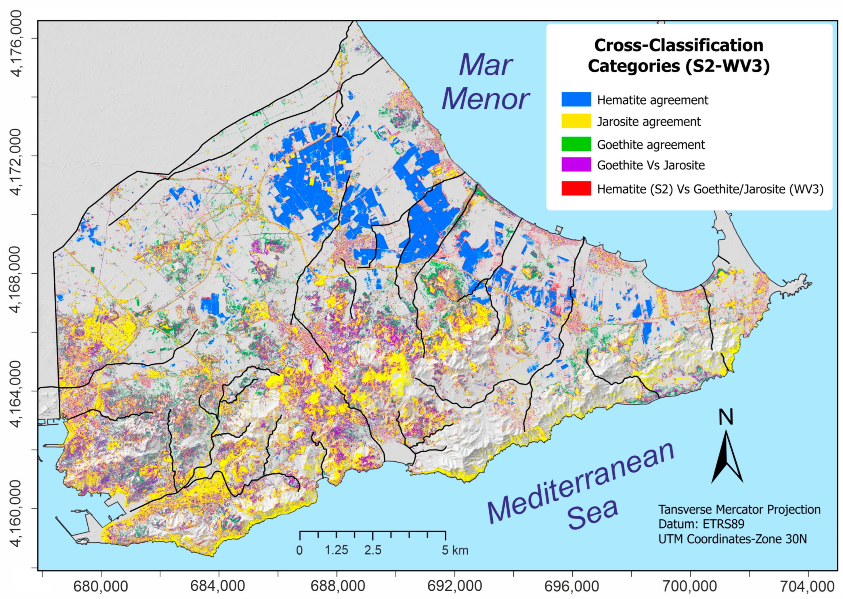
The cross-tabulation between S2 and WV3 discrete classifications derived from the composition band ratio is presented in

Table 11. Cross-tabulation of S2 and WV3 mineral classes derived from the composition band ratio. Values are expressed in MP: 1 MP = 1,000,000 pixels and hectares (ha). Values in parentheses represent percentages relative to the total number of analyzed pixels (60,046,506 pixels; 9228 ha).

			Sentinel-2
			Hematite	Goethite	Jarosite
WorldView-3	Hematite	MP (%)	17.86 (29.7%)	0.27 (0.5%)	0.34 (0.6%)
		ha	2746	42	52
	Goethite	MP (%)	1.40 (2.3%)	8.41 (14.0%)	11.36 (18.9%)
		ha	215	1293	1747
	Jarosite	MP (%)	1.50 (2.5%)	3.85 (6.4%)	15.05 (25.1%)
		ha	231	592	2314

; the spatial distribution of agreement and disagreement is shown in Figure 10. A total of 60.05 megapixels (MP; 60,046,506 pixels; 9222 ha) were compared in this analysis, based on the WV3-resolution grid following resampling of S2 classifications. As explained in Section 2.5, pixel counts are based on the WV3-resolution grid following the resampling procedure.

Overall intersensor agreement amounts to 41.32 MP, corresponding to 68.8% of the total analyzed pixels, which indicates a high level of consistency between both sensors for this approach (Table 11).

Hematite shows the highest intersensor agreement, with 17.86 MP (29.7%) being classified consistently by both sensors. Figure 10 shows these coincident pixels in blue, forming large and continuous areas in the downstream Mar Menor sector of the study area. Goethite and jarosite also show a notable agreement, with 8.41 MP (14.0%) for the former and 15.05 MP (25.0%) for the latter. These coincidence areas, shown in green and yellow, respectively, in Figure 10, are found mainly alongside drainage channels and in the headwater sectors.

The main disagreement corresponds to reciprocal differences between goethite and jarosite: 11.36 MP (18.9%) classified as goethite in the WV3 composition band ratio correspond to jarosite in the S2 one, whereas 3.85 MP (6.4%) classified as jarosite in the WV3 composition band ratio correspond to goethite in the S2 one. These mismatches are represented in purple in Figure 10 and are observed mainly in the headwater sections and along drainage channels. Additionally, 2.90 MP (4.8%) classified as hematite in the S2 composition band ratio are identified as goethite (1.40 MP; 2.3%) or jarosite (1.50 MP; 2.5%) in the WV3 one. These areas, shown in red in Figure 10, concentrate mainly at the boundaries of hematite-dominated zones and along drainage channels.

3.4.2. Parabola Fitting Technique: Cross-Sensor Comparison

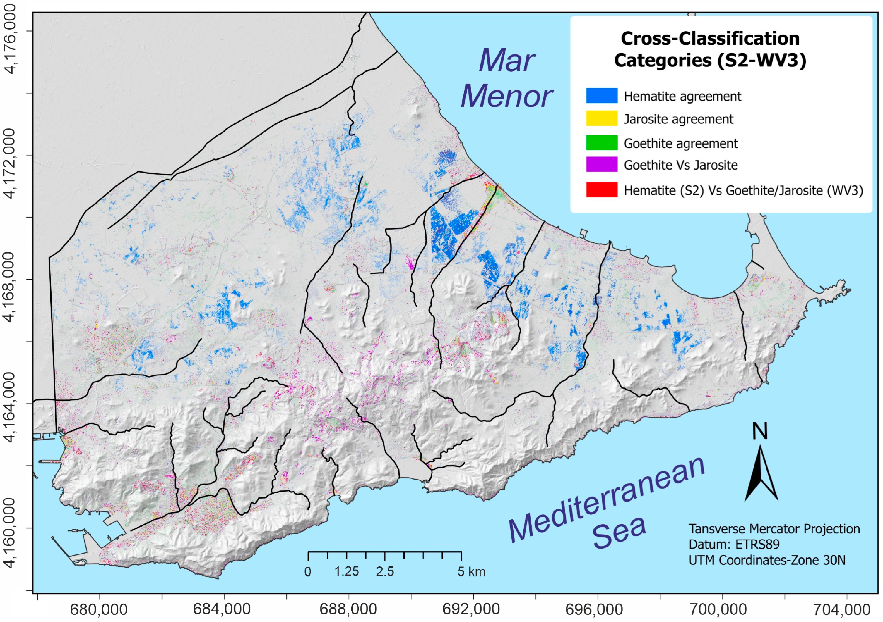
The cross-tabulation between S2 and WV3 classifications derived from the parabola fitting technique is presented in

Table 12. Cross-tabulation of S2 and WV3 mineral classes derived from the parabola fitting technique. Values are expressed in MP: 1 MP = 1,000,000 pixels and hectares (ha). Values in parentheses represent percentages relative to the total number of analyzed pixels (6,869,015 pixels; 1056 ha).

			Sentinel-2
			Hematite	Goethite	Jarosite
WorldView-3	Hematite	MP (%)	4.93 (76.3%)	0.05 (0.8%)	0.03 (0.5%)
		ha	758	8	5
	Goethite	MP (%)	0.22 (3.4%)	0.21 (3.3%)	0.01 (0.2%)
		ha	34	32	2
	Jarosite	MP (%)	0.35 (5.4%)	0.17 (2.6%)	0.49 (7.6%)
		ha	54	26	75

, and the corresponding spatial agreement is shown in Figure 11. In this case, 6.87 MP (6,869,015 pixels; 1056 ha) were compared, based on the WV3-resolution grid. This was a number substantially lower than that used in the composition band ratio analysis (60.05 MP; 9222 ha). As explained in Section 2.5, pixel counts are based on the WV3-resolution grid following the resampling procedure. This smaller quantity of pixels analyzed mainly reflects the limited spatial extent of the WV3 classifications derived from the parabola fitting approach (Figure 8).

The overall intersensor agreement reaches 5.63 MP (87.2%) of the total analyzed pixels. However, this high proportional agreement is strongly controlled by the dominant contribution of hematite coincidence (4.93 MP; 76.3%), which reflects the limitation of the WV3 parabola fitting approach to identify goethite and jarosite (Figure 4 and Figure 8B).

As in the composition band ratio comparison, hematite shows the highest level of agreement, with 4.93 MP (76.3%) classified as hematite by both sensors. These coincident pixels form large continuous areas in the downstream sector of the Mar Menor and are represented in blue in Figure 11. The agreement for goethite (0.21 MP; 3.3%) and jarosite (0.49 MP; 7.6%) is lower than that obtained with the composition band ratio method (Table 12), and is also more spatially restricted. These coincident areas (shown in green and yellow, respectively, in Figure 11) are observed mainly next to drainage sectors.

The dominant disagreement corresponds to pixels classified as hematite in the S2 parabola fitting technique results but as jarosite (0.35 MP; 5.4%) or goethite (0.22 MP; 3.4%) in the WV3 classification. These areas are shown in red in Figure 11 and are scattered along drainage channels. Overall, reciprocal differences between goethite and jarosite are limited and appear as small, localized purple patches in Figure 11. These predominantly correspond to pixels classified as goethite in the S2 parabola fitting technique but as jarosite in the WV3 classification (0.17 MP; 2.6%).

4. Discussion

In the present study, the performance of the S2 and WV3 multispectral sensors is evaluated for mapping and discriminating secondary iron minerals associated with AMD in the post-mining landscape of the Sierra Minera de Cartagena–La Unión. The results show the influence of sensor design, particularly the trade-off between spectral and spatial resolution, as well as the methodological approach, on the detectability and discrimination of minerals in post-mining environments, as reported in previous studies [9,10,33].

Composition band ratio maps (Figure 7) provided broad mineral distribution patterns. For S2, the results showed a high level of agreement with XRD validation data, with 61 of the 74 samples correctly classified (82.4%; Table 4 and Table 5). However, the reliability of the WV3 composition band ratio was lower, with 55 correctly classified samples (74.3%) and a higher number of misclassifications (16.2%). In samples containing mixed mineral assemblages, it frequently failed to identify the predominant iron phase and occasionally assigned one of the three studied iron minerals to pixels for which XRD detected none (Table 4). However, these overall agreement values include the 33 non-target samples, which are correctly unclassified in most and therefore increase the overall metric. When performance is evaluated exclusively on the 41 target-mineral samples, accuracy drops to 73.2% for S2 band ratio and 58.5% for WV3 band ratio (Table 10).

The results are consistent with previous studies that describe composition band ratio techniques as first-order approximations of mineral distribution [10,15,34]. Their main advantage lies in their computational efficiency, as they can be easily applied to large datasets, making them suitable for regional monitoring. However, composition band ratio classifications are inherently sensitive to threshold selection, which may influence the resulting mineral distribution patterns [10,15,34]. The sensitivity analysis presented in Table 2 and Table 3 confirms this. Narrowing the thresholds substantially reduces the number of correctly detected target minerals because more samples fall outside the defined ranges and remain unclassified. In contrast, widening the thresholds does not improve mineral detection but progressively increases the number of false positives by assigning non-target samples to mineral classes. This indicates that the selected thresholds provide the best balance between detecting the target minerals and limiting false positives for the conditions of this study.

The parabola fitting technique showed greater potential for mineral discrimination, although its effectiveness was sensor-dependent; when applied to the S2 image, the narrow red-edge and NIR bands (B5–B8A) enabled the accurate interpolation of diagnostic peaks, resulting in 60 correctly classified samples (81.1%), three misclassifications (4.1%), and 11 unclassified cases (14.9%) relative to XRD results (Table 4 and Table 5). The fitted parabolas for S2 spectral curves showed a strong match with laboratory spectra, allowing reliable mineral separation even with a multispectral resolution. These findings align with earlier studies, which demonstrated that the spectral configuration of S2, particularly the red-edge bands, enables the adaptation of feature-based methods originally developed for hyperspectral data [8,34]. Such approaches are typical in hyperspectral remote sensing, where the high spectral resolution allows detailed characterization of diagnostic absorption features [9,35,36], which are directly linked to mineral composition. Their transfer to multispectral sensors has proven effective when band positioning adequately samples the absorption feature [8,34], enabling mineral identification even with reduced spectral resolution. In this study, a novel adaptation of the technique to reflectance maxima proved effective in differentiating goethite and jarosite, something that could not be achieved using absorption features, as their absorption minima are spectrally very similar [8]. Furthermore, constructing parabolas for reflectance maxima avoided using band 9, which is required for the absorption-based approach. Since band 9 in the S2 sensor has the lowest spatial resolution (60 m), excluding it prevented degradation of the spatial resolution. However, a limitation of adapting the technique to reflectance maxima is that this method does not allow for mineral quantification, which is possible using the absorbance minima [8].

For WV3, the parabola fitting technique showed the greatest discrepancies with the XRD results, with 53 correctly classified samples (71.6%), six misclassifications (8.1%), and 15 unclassified samples (20.3%; Table 4 and Table 5). It only achieved partial discrimination, mainly between hematite and the goethite–jarosite group. This limitation can be attributed to both the spectral configuration of WV3 in the VNIR, which includes fewer bands than S2—particularly in the red-edge and NIR regions—and to the absence of SWIR data in this study. The SWIR range of WV3 covers diagnostic vibrational absorption features of hydroxyl- and sulphate-bearing minerals, including jarosite, which could help with the discrimination of both jarosite and goethite [33,37,38]. Future work should examine the potential of WV3 SWIR bands for AMD mineral mapping, particularly for exploiting the diagnostic jarosite absorption feature near 2.27 µm. Integrating SWIR and VNIR data has been shown to significantly enhance mineral discrimination in AMD-affected and hydrothermal alteration environments [14,15,16].

When the analysis was restricted to the 41 target-mineral samples, target-mineral accuracy decreased from 81.1% to 70.7% for S2 parabola fitting and from 71.6% to only 48.8% for WV3 parabola fitting (Table 10). This further highlights the limited capacity of WV3 VNIR data to discriminate among the three iron minerals. Despite its lower spectral discrimination capacity in the VNIR region, WV3 offered advantages in terms of spatial detail. Its 1.24 m spatial resolution allows improved characterization of fine-scale mineral variability in highly heterogeneous environments, such as narrow drainage channels and ramblas, where AMD-related materials appear as discontinuous patches. These channelized areas are usually dominated by the presence of goethite and jarosite under acidic and fluctuating hydrological conditions, while hematite is generally absent. Accurate spatial characterization of these zones is therefore important to identify areas of active oxidation and ongoing AMD processes [35,39]. This spatial behavior is reflected in the cross-sensor comparison (Figure 10), in which discrepancies are associated mainly with pixels classified as hematite in S2 results but assigned to goethite or jarosite in WV3 results, especially along drainage channels adjacent to hematite-dominated surfaces.

In such confined environments, the 10 m spatial resolution of S2 can result in mixed pixels that integrate the spectral responses of adjacent materials, including surrounding hematite-rich deposits. This spatial averaging effect can mask small-scale mineral variability and reduce discrimination performance in narrow channelized sectors [9]. In contrast, while WV3 data could not be used to reliably separate goethite from jarosite using VNIR data alone, goethite–jarosite assemblages could successfully be differentiated from hematite. This capability is particularly relevant in these channel areas, where distinguishing the absence of hematite from adjacent hematite-dominated zones improves the spatial interpretation of active AMD-related mineralization. Similar results have been reported in WV3 VNIR studies, where iron oxide and hydroxide assemblages can be distinguished at high spatial resolution, even when mineral-level separation remains limited [15].

The differences observed between S2 and WV3 should also be interpreted by considering several additional sources of uncertainty. In addition to spectral and spatial resolution, differences in sensor radiometric performance, including signal-to-noise ratio, may influence the detection of subtle spectral features [9,34]. In addition, although vegetation and water masks were applied before mineral mapping, residual spectral interference from dry or senescent vegetation cannot be completely excluded. This is especially relevant in semi-arid environments, where sparse or dry vegetation may show low NDVI values and remain within the exposed-soil mask [26]. Such residual vegetation may affect both ratio values and parabola-derived classifications when mixed with soils and mine wastes in the VNIR region [26].

Another limitation to consider is that the parabola fitting optimization was based on one representative laboratory spectrum for each mineral. Although these spectra were selected from XRD-confirmed samples dominated by hematite, goethite, and jarosite, they do not capture the full spectral variability that may result from grain size, hydration state, mineral mixtures, coatings, or surface conditions. This variability may partly affect the position and shape of the reflectance maximum and, therefore, the classification results.

A further consideration concerns the partial overlap between the calibration and validation samples used for the parabola fitting technique, since SM-005, SM-060, and SM-011 were used to optimize the band combination and were also included in the validation dataset. However, calibration relied on ASD laboratory reflectance spectra acquired under controlled indoor conditions, whereas validation compared satellite-derived pixel classifications, obtained under real atmospheric and illumination conditions, with XRD-determined mineral identities. These independent measurements of the same physical samples reduce the risk of circular validation. Nevertheless, a slight optimistic bias for these three samples cannot be completely excluded, and future work should consider a fully independent validation design. Finally, threshold selection is another important source of uncertainty, particularly for the composition band ratio approach, where thresholds directly control the apparent extent of the mapped mineral classes [30,31]. For this reason, the classified classes should be interpreted as dominant spectral responses rather than definitive mineralogical boundaries [15,32]. For the parabola fitting technique, the classification was based only on the wavelength position of the reflectance maximum [8,32]. The intensity and shape of the fitted peak were not used to estimate mineral abundance because their relationship with mineral abundance is less direct than in approaches based on absorption depth or reflectance minima [8,31]. Therefore, their use for defining refined thresholds or estimating relative abundance would require specific calibration against quantitative mineralogical data and could be explored in future work.

Overall, despite its coarse resolution, the S2 VNIR bands performed better than the WV3 VNIR bands in the spectral discrimination of hematite, goethite, and jarosite (Figure 5, Figure 7 and Figure 8, Table 4), particularly when the parabola fitting technique was applied (Figure 8). This improved performance is due to the configuration of S2 narrow red-edge and NIR bands, which align well with diagnostic reflectance peaks of iron oxides and hydroxides (Figure 1). Such band configuration allows the detection of subtle shifts in the spectral position of iron reflectance maxima [10,11,35]. WV3, despite offering a higher spatial resolution, is limited in the VNIR range by having a single red-edge band and broader NIR and red bands, which restricts its ability to separate goethite from jarosite (Table 4), though it could be used to differentiate the goethite–jarosite group from hematite.

Similar relationships between sensor characteristics and mineral detectability have been observed in other AMD-affected environments [9,35,40]. In SE Spain, as well as in the Iberian Pyrite Belt, hyperspectral studies have shown that hematite, goethite, and jarosite can be accurately identified due to their distinct spectral features [35,39], whereas multispectral approaches are more limited when spectral resolution is insufficient [9,39]. In other mining environments worldwide, composition band ratio techniques have been widely used for rapid mapping of iron-rich materials [9,15], although their performance is affected by spectral mixing and threshold selection [15,32]. These studies highlight the importance of combining spectral and spatial information, as well as integrating multiple sensors, to improve mineral discrimination in complex mining landscapes.

From a mining management perspective, these findings underline the complementary value of both sensors. S2 provides a cost-effective approach for the systematic large-scale monitoring of oxidation processes and the identification of potential contamination-prone areas, while commercial WV3 offers enhanced spatial detail in areas of high mineralogical variability. Together, these capabilities support environmental management, remediation planning, and more sustainable governance in both abandoned and active mining districts.

5. Conclusions

Our results suggest that both the S2 sensor and the WV3 sensor are able to capture the general spatial distribution of secondary iron minerals, hematite, goethite, and jarosite, associated with AMD in southeastern Spain. However, S2 obtained a higher agreement with XRD results, in particular with the parabola fitting technique approach. This indicates that S2 performed well not only in identifying the presence or absence of the target iron minerals, but also in discriminating among hematite, goethite, and jarosite. Its narrow red-edge and NIR bands are well positioned to capture subtle shifts in reflectance maxima, enabling improved discrimination of the three iron minerals despite its 10 m spatial resolution. These results highlight the importance of spectral configuration for discriminating spectrally similar minerals.

However, this discriminatory capability should be interpreted in terms of class-specific performance. Hematite was consistently well detected across all methods, with recall values between 66.7% and 77.8%, whereas goethite and jarosite showed greater variability and were more prone to mutual confusion, particularly in mixed mineral assemblages. In addition, the overall agreement values were substantially influenced by the correct non-classification of the 33 non-target samples. When only the 41 target-mineral samples were considered, accuracy decreased from 82.4% to 73.2% for the S2 band ratio and from 81.1% to 70.7% for the S2 parabola fitting technique.

Band ratio results were useful for identifying broad mineral distribution patterns, but they should be interpreted as dominant spectral responses rather than definitive mineral identifications. In contrast, the parabola fitting technique provided a more robust basis for mineral discrimination because it used the wavelength position of the reflectance maximum, which is directly linked to the spectral behavior of the target minerals.

WV3 VNIR data allowed only partial discrimination, mainly differentiating hematite from the goethite–jarosite group. Nevertheless, its 1.24 m spatial resolution provided improved delineation of narrow drainage channels and ramblas, in which goethite and jarosite appear together and hematite is generally absent. In such confined environments, the S2 10 m resolution may lead to mixed pixels that mask small-scale mineral variability.

Overall, S2 offers a cost-effective tool for large-scale AMD monitoring and the identification of areas with secondary iron mineral accumulation that may indicate contamination risk, while WV3 provides enhanced spatial detail for site-specific assessments. Together, both sensors support a more sustainable management of mining-impacted landscapes.

References

1. Nordstrom, D.K.; Alpers, C.N. Negative pH, efflorescent mineralogy, and consequences for environmental restoration at the Iron Mountain Superfund Site, California. Proc. Natl. Acad. Sci. USA 1999, 96, 3455–3462. [Google Scholar] [CrossRef] [PubMed]
2. Nordstrom, D.K.; Blowes, D.W.; Ptacek, C.J. Hydrogeochemistry and microbiology of mine drainage: An update. Appl. Geochem. 2015, 57, 3–16. [Google Scholar] [CrossRef]
3. Bott, T.L.; Jackson, J.K.; McTammany, M.E.; Newbold, J.D.; Rier, S.T.; Sweeney, B.W.; Battle, J.M. Abandoned coal mine drainage and its remediation: Impacts on stream ecosystem structure and function. Ecol. Appl. 2012, 22, 2144–2163. [Google Scholar] [CrossRef] [PubMed]
4. Madejón, P.; Caro-Moreno, D.; Navarro-Fernández, C.M.; Rossini-Oliva, S.; Marañón, T. Rehabilitation of waste rock piles: Impact of acid drainage on potential toxicity by trace elements in plants and soil. J. Environ. Manag. 2021, 280, 111848. [Google Scholar] [CrossRef] [PubMed]
5. Hammarstrom, J.M.; Seal, R.R., II; Meier, A.L.; Kornfeld, J.M. Secondary sulfate minerals associated with acid drainage in the eastern United States: Recycling of metals and acidity in surficial environments. Chem. Geol. 2005, 215, 407–431. [Google Scholar]
6. Singer, R.B. Near-infrared spectral reflectance of mineral mixtures: Systematic combinations of pyroxenes, olivine, and iron oxides. J. Geophys. Res. Solid Earth 1981, 86, 7967–7982. [Google Scholar] [CrossRef]
7. Rossman, G.R.; Ehlmann, B.L. Electronic spectra of minerals in the visible and near-infrared regions. In Remote Compositional Analysis: Techniques for Understanding Spectroscopy, Mineralogy, and Geochemistry of Planetary Surfaces; Cambridge University Press: Cambridge, UK, 2019; pp. 3–20. [Google Scholar] [CrossRef]
8. van der Werff, H.; van der Meer, F. Sentinel-2 for mapping iron absorption feature parameters. Remote Sens. 2015, 7, 12635–12653. [Google Scholar] [CrossRef]
9. Kruse, F.A.; Perry, S.L.; Caballero, A. Mineral mapping using WorldView-3 satellite data. Remote Sens. 2013, 7, 6730–6751. [Google Scholar] [CrossRef]
10. Pereira, I.; Alcalde-Aparicio, S.; Ferrer-Julià, M.; Carreño, M.F.; García-Meléndez, E. Monitoring sedimentary areas from mine waste products with Sentinel-2 satellite images: A case study in the SE of Spain. Eur. J. Soil Sci. 2023, 74, e13336. [Google Scholar] [CrossRef]
11. Soydan, H.; Koz, A.; Düzgün, H.Ş. Secondary iron mineral detection via hyperspectral unmixing analysis with Sentinel-2 imagery. Int. J. Appl. Earth Obs. Geoinf. 2021, 101, 102343. [Google Scholar] [CrossRef]
12. Hosseinjanizadeh, M.; Khorasanipour, M.; Honarmand, M. Mapping mining waste and identification of acid mine drainage within an active mining area through sub-pixel analysis on OLI and Sentinel-2. Earth Sci. Inform. 2023, 16, 3449–3467. [Google Scholar] [CrossRef]
13. Pereira, I.; García-Meléndez, E.; Ferrer-Julià, M.; van der Werff, H.; Valenzuela, P.; Cruz, J.A. Multi-temporal mineral mapping in two torrential basins using PRISMA hyperspectral imagery. Remote Sens. 2025, 17, 2582. [Google Scholar] [CrossRef]
14. Sun, Y.; Tian, S.; Di, B. Extracting mineral alteration information using WorldView-3 data. Geosci. Front. 2017, 8, 1051–1062. [Google Scholar] [CrossRef]
15. Salehi, T.; Tangestani, M.H. Evaluation of WorldView-3 VNIR and SWIR data for hydrothermal alteration mapping for mineral exploration: Case study from northeastern Isfahan, Iran. Nat. Resour. Res. 2020, 29, 3479–3503. [Google Scholar] [CrossRef]
16. Park, H.; Choi, J. Mineral detection using sharpened VNIR and SWIR bands of WorldView-3 satellite imagery. Sustainability 2021, 13, 5518. [Google Scholar] [CrossRef]
17. United States Geological Survey. Spectral Library. 2017. Available online: https://www.usgs.gov/labs/spectroscopy-lab/science/spectral-library (accessed on 18 January 2026).
18. García, C. Impacto y Riesgo Ambiental de los Residuos Minero-Metalúrgicos de la Sierra de Cartagena–La Unión (Murcia, España). Ph.D. Thesis, Universidad Politécnica de Cartagena, Cartagena, Spain, 2004. Available online: https://repositorio.upct.es/entities/publication/c0907d15-3c6d-479a-a40d-7ae65ff029b0 (accessed on 9 January 2026).
19. López-Morell, M.Á.; Pérez de Perceval Verde, M.Á. From old mining to new mining: The introduction of differential flotation in Spanish mines and its environmental impact. Rev. Hist. Ind.—Ind. Hist. Rev. 2019, 28, 119–148. [Google Scholar] [CrossRef]
20. Alonso Sarriá, F.; López Bermúdez, F.; Conesa García, C. Synoptic conditions producing extreme rainfall events along the Mediterranean coast of the Iberian Peninsula. In Dryland Rivers: Hydrology and Geomorphology of Semi-Arid Channels; John Wiley & Sons: Chichester, UK, 2002; pp. 351–371. [Google Scholar]
21. Pacifici, F. Atmospheric Compensation in Satellite Imagery. U.S. Patent 9,396,528 B2, 19 July 2016. [Google Scholar]
22. Richter, R.; Louis, J.; Müller-Wilm, U. Sentinel-2 MSI—Level 2A Products Algorithm Theoretical Basis Document; S2PAD-ATBD-0001, Issue 2.0; Telespazio VEGA Deutschland GmbH: Darmstadt, Germany, 2012. [Google Scholar]
23. Brodu, N. Super-resolving multiresolution images with band-independent geometry of multispectral pixels. IEEE Trans. Geosci. Remote Sens. 2017, 55, 4610–4617. [Google Scholar]
24. DigitalGlobe. WorldView-3 Data Sheet; DigitalGlobe Inc.: Westminster, CO, USA, 2014. [Google Scholar]
25. Drusch, M.; Del Bello, U.; Carlier, S.; Colin, O.; Fernandez, V.; Gascon, F.; Hoersch, B.; Isola, C.; Laberinti, P.; Martimort, P.; et al. Sentinel-2: ESA’s Optical High-Resolution Mission for GMES Operational Services. Remote Sens. Environ. 2012, 120, 25. [Google Scholar] [CrossRef]
26. Rouse, J.W.; Haas, R.H.; Schell, J.A.; Deering, D.W. Monitoring vegetation systems in the Great Plains with ERTS. In Proceedings of the Third ERTS-1 Symposium; NASA SP-351; Washington, DC, USA, December 1973; National Aeronautics and Space Administration (NASA): Washington, DC, USA, 1974; Volume I, pp. 309–317. [Google Scholar]
27. McFeeters, S.K. The use of the Normalized Difference Water Index (NDWI) in the delineation of open water features. Int. J. Remote Sens. 1996, 17, 1425–1432. [Google Scholar] [CrossRef]
28. Rowan, L.C.; Mars, J.C. Lithologic mapping in the Mountain Pass, California area using Advanced Spaceborne Thermal Emission and Reflection Radiometer (ASTER) data. Remote Sens. Environ. 2003, 84, 350–366. [Google Scholar] [CrossRef]
29. Sahwan, W.; Lucke, B.; Sprafke, T.; Vanselow, K.A.; Bäumler, R. Relationships between spectral features, iron oxides and colours of surface soils in northern Jordan. Eur. J. Soil Sci. 2020, 72, 80–97. [Google Scholar] [CrossRef]
30. Rowan, L.C.; Mars, J.C.; Simpson, C.J. Lithologic mapping of the Mordor, NT, Australia ultramafic complex using the Advanced Spaceborne Thermal Emission and Reflection Radiometer (ASTER). Remote Sens. Environ. 2005, 99, 105–126. [Google Scholar] [CrossRef]
31. Cudahy, T. Australian ASTER Geoscience Product Notes, Version 1; CSIRO ePublish No. EP-30-07-12-44; CSIRO: Canberra, Australia, 2012.
32. Pereira, I.; Ferrer-Julià, M.; van der Werff, H.; García-Meléndez, E.; Valenzuela, P.; Colmenero-Hidalgo, E.; Cruz, J.A.; van der Meer, F. Cartografía del máximo de reflectancia de minerales de hierro con Sentinel-2: Un caso de estudio en la Sierra Minera de Cartagena. In Teledetección y Cambio Global: Retos y Oportunidades para un Crecimiento Azul. XX Congreso de la Asociación Española de Teledetección; Caballero, I., Navarro, G., Barbero, L., Gómez-Enri, J., Eds.; Editorial UCA: Cádiz, Spain, 2024; ISBN 978-84-9828-941-1. [Google Scholar]
33. Crowley, J.K.; Williams, D.E.; Hammarstrom, J.M.; Piatak, N.M.; Chou, I.-M.; Mars, J.C. Spectral reflectance properties (0.4–2.5 µm) of secondary Fe-oxide, Fe-hydroxide, and Fe-sulfate-hydrate minerals associated with sulfide-bearing mine wastes. Geochem. Explor. Environ. Anal. 2003, 3, 219–228. [Google Scholar] [CrossRef]
34. Mielke, C.; Boesche, N.K.; Rogass, C.; Kaufmann, H.; Gauert, C.; De Wit, M. Spaceborne mine waste mineralogy monitoring in South Africa, applications for modern push-broom missions: Hyperion/OLI and EnMAP/Sentinel-2. Remote Sens. 2014, 6, 6790–6816. [Google Scholar] [CrossRef]
35. Ge, W.; Cheng, Q.; Jing, L.; Wang, F.; Zhao, M.; Ding, H. Assessment of the capability of Sentinel-2 imagery for iron-bearing minerals mapping: A case study in the Cuprite area, Nevada. Remote Sens. 2020, 12, 3028. [Google Scholar] [CrossRef]
36. Buzzi, J.; Riaza, A.; García-Meléndez, E.; Weide, S.; Bachmann, M. Mapping changes in a recovering mine site with hyperspectral airborne HyMap imagery (Sotiel, SW Spain). Minerals 2014, 4, 313–329. [Google Scholar] [CrossRef]
37. Asadzadeh, S.; Zhou, X.; Chabrillat, S. Assessment of the spaceborne EnMAP hyperspectral data for alteration mineral mapping: A case study of the Reko Diq porphyry CuAu deposit, Pakistan. Remote Sens. Environ. 2024, 314, 114389. [Google Scholar]
38. Bedini, E.; Chen, J. Prospection for economic mineralization using PRISMA satellite hyperspectral remote sensing imagery: An example from central East Greenland. J. Hyperspectral Remote Sens. 2022, 12, 124–130. [Google Scholar] [CrossRef]
39. Riaza, A.; Buzzi, J.; García-Meléndez, E.; Carrère, V.; Müller, A. Monitoring the extent of contamination from acid mine drainage in the Iberian Pyrite Belt (SW Spain) using hyperspectral imagery. Remote Sens. 2011, 3, 2166–2186. [Google Scholar] [CrossRef]
40. Mars, J.C.; Rowan, L.C. Spectral assessment of new ASTER SWIR surface reflectance data products for spectroscopic mapping of rocks and minerals. Remote Sens. Environ. 2010, 114, 2011–2025. [Google Scholar] [CrossRef]
Figure 2. Overview of the Sierra Minera de Cartagena–La Unión study area in southeastern Spain. The inset map shows the location of the study area within the Region of Murcia and the Iberian Peninsula. (A) Panoramic view of the Sierra Minera de Cartagena–La Unión showing extensive mine waste deposits. (B) View of the Campo de Cartagena agricultural plain located north of the mining district. (C) Rambla del Beal draining towards the Mar Menor lagoon, characterized by gentle slopes. (D) Rambla del Gorguel draining into the Mediterranean Sea, showing steeper slopes and more confined channel morphology.
Remotesensing 18 02240 g002
Figure 3. Spectral reflectance curves of representative iron oxides and hydroxides (hematite, jarosite, and goethite) in the visible range, highlighting the green (∼550–600 nm) and red (∼650–700 nm) wavelength regions used in the composition band ratio. Spectral data were obtained from [17]: Hematite GDS76, Goethite WS222, and Jarosite GDS99 K-y 200C.
Remotesensing 18 02240 g003
Figure 4. Spectra of hematite, goethite, and jarosite for (A) S2 and (B) WV3 data. ASD spectra (blue line), S2 or WV3 bands (blue dots), fitted parabola (black line), and deduced wavelength of maximum reflectance (purple dot for S2 and orange dot for WV3). Validation and field data collection.
Remotesensing 18 02240 g004
Figure 5. Location of the collected samples.
Remotesensing 18 02240 g005
Figure 6. Distribution of red/green band ratio values across the study area for (A) Sentinel-2 (B4/B3) and (B) WorldView-3 (B5/B3). Ratio values range from 0.6 to 4.0. Gray bars = pixel frequency distribution; colored bars = applied classification threshold ranges (goethite: 0.6–0.9; jarosite: 1.8–2.1; hematite: 3.3–3.5). Colored dots = ratio values extracted at the 74 validation sample locations, colored by the XRD reference class.
Remotesensing 18 02240 g006
Figure 7. (A) Iron oxide and hydroxide composition ratio (B4/B3) for S2 and (B) iron oxide and hydroxide composition ratio (B5/B3) for WV3.
Remotesensing 18 02240 g007
Figure 8. Parabola fitting technique. Reflectance feature parameter wavelength maximum reflectance for (A) S2 and (B) WV3.
Remotesensing 18 02240 g008
Figure 9. Examples of diffractogram and identified phase (Clct: calcite; Gpsm: gypsum; Gth: goethite; Hem: hematite; Ilt: illite; Jrs: jarosite; Kln: kaolinite; Qrtz: quartz).
Remotesensing 18 02240 g009
Figure 10. Spatial agreement between S2 and WV3 discrete mineral classifications derived from the composition band ratio. Blue, green, and yellow indicate areas where both sensors classify the same mineral (hematite, goethite, and jarosite, respectively). Purple represents areas where one sensor classifies goethite and the other jarosite. Red highlights pixels classified as hematite in the S2 composition band ratio but as goethite or jarosite in the WV3 ones.
Remotesensing 18 02240 g010
Figure 11. Spatial agreement between S2 and WV3 mineral classifications derived from the parabola fitting technique. Blue, green, and yellow indicate areas where both sensors classify the same mineral (hematite, goethite, and jarosite, respectively). Purple represents areas where one sensor classifies goethite and the other jarosite. Red highlights pixels classified as hematite in the S2 parabola fitting technique but as goethite or jarosite in the WV3 parabola fitting technique.
Remotesensing 18 02240 g011