DST-SARNet: A Dual-Stage Texture-Aware SAR Prior Network for Cloud Removal in Optical Remote Sensing Images

Highlights

What are the main findings?

• We propose DST-SARNet, a dual-stage texture-aware SAR prior network for thick-cloud removal. Instead of performing dense multi-layer SAR fusion, DST-SARNet organizes SAR information into early structural skeletons, deep texture memory, and late high-frequency modulation signals for controlled SAR-assisted optical reconstruction.
• DST-SARNet combines structure–appearance decoupling, efficient global context modeling, and Texture-Aware Asymmetric Retrieval to improve structural recovery, detail preservation, and visual consistency in thick-cloud regions while reducing the propagation of SAR speckle noise and cross-modal misalignment.

What are the implications of the main findings?

• The experimental results show that effective SAR-assisted cloud removal does not necessarily require layer-by-layer dense fusion. Transforming SAR observations into controlled structural priors and detail modulation signals preserves cloud-hidden surface texture cues while reducing the cumulative propagation of speckle noise, local registration perturbations, and cross-modal imaging discrepancies.
• The proposed framework achieves a favorable balance among reconstruction quality, structural fidelity, and computational efficiency, providing a practical technical route for the efficient restoration of large-scale cloud-contaminated optical remote sensing imagery and subsequent surface monitoring applications.

Abstract

Cloud contamination obscures ground objects, interferes with surface reflectance, and disrupts spatial continuity. In thick-cloud regions, surface structures and spectral information are often extensively missing. CNN-based cloud removal methods can recover local textures, but they are less effective at modeling global structures and color consistency over large cloud-covered areas. Transformer-based methods capture long-range dependencies; however, standard self-attention introduces high computational and memory costs for high-resolution remote sensing images. Efficient attention reduces this cost but may weaken edge and texture discriminability. SAR imagery can penetrate clouds and provide surface structural information, yet repeated SAR injections may propagate speckle noise, cross-modal misalignment, and imaging discrepancies through deep restoration layers. To address these issues, this paper proposes DST-SARNet, a dual-stage SAR structural guidance network for optical remote sensing image cloud removal. In this framework, dual-stage refers to two explicit SAR-guidance positions: early structural skeleton guidance at the input side and late high-frequency modulation near the output. The Texture-Aware Asymmetric Retrieval module is placed between these two stages as a bottleneck memory retrieval operation rather than as a third dense SAR injection stage. With this design, SAR provides structural skeletons, readable texture memory, and terminal detail compensation, while the optical branch remains responsible for color, semantics, and spectral appearance recovery. Experiments on the SMILE-CR and SEN12MS-CR datasets show that DST-SARNet effectively restores cloud-contaminated imagery with a compact model scale, demonstrating its potential for efficient SAR-assisted optical cloud removal.

1. Introduction

Optical remote sensing imagery provides wide-area coverage, rich spectral information, and intuitive visual interpretability, making it an important data source for Earth observation. Optical satellite missions such as Landsat-8 and Sentinel-2 support land-cover mapping, agricultural monitoring, urban planning, disaster assessment, environmental observation, and long-term ecological evaluation [1,2]. The value of these images depends on continuous surface observations and reliable reflectance information, both of which are disrupted by cloud contamination. Thin clouds reduce local contrast and introduce haze-like interference, whereas thick clouds can completely obscure surface structures and make original spectral information unavailable. Accordingly, cloud and cloud-shadow detection studies, including recent self-attention and spatial-pyramid-pooling-based methods, regard cloud contamination as a central quality-control problem in optical remote sensing products [3,4,5].

The objective of remote sensing image cloud removal is to reconstruct cloud-free optical imagery from cloud-contaminated observations. Existing methods can generally be grouped into single-image inpainting, multi-temporal reconstruction, and multimodal fusion [6,7,8,9]. Single-image inpainting methods infer missing regions from spatial continuity and semantic similarity within the same cloudy image. Classical image inpainting and missing-information reconstruction in remote sensing provide the foundation for this category [6,7]. These methods require limited auxiliary data and are useful when cloud coverage is small or sufficient contextual information remains around clouds. Their limitations become evident when large cloud masses cover complex surface regions. Buildings, roads, coastlines, rivers, fragmented farmland, and mountainous terrain contain complex structures, and the visible content in a single optical image is often insufficient to recover true surface morphology, leading to over-smoothed or semantically inconsistent outputs.

Multi-temporal methods use cloud-free or less-cloudy observations acquired at different dates to supplement missing information. When reliable observations of the same region are available from adjacent dates, they provide direct references for obscured regions and are useful for long-term time-series monitoring [7,8]. In practice, however, suitable temporal references are not always available. Seasonal variation, crop growth, urban construction, water-level changes, phenology, and registration errors can introduce inconsistent spectral or structural information. If the land cover changes between the reference and target dates, the reconstructed result may inherit outdated surface patterns. This difficulty becomes more evident in rapidly changing areas or under persistent cloudy weather. Related studies on adverse-condition change detection and haze/mosaic simulation also indicate that degraded optical observations reduce the reliability of temporal interpretation and downstream change analysis [10,11].

Multimodal methods alleviate information loss caused by cloud cover by introducing complementary observations from different sensors. Synthetic aperture radar (SAR) provides all-day and all-weather imaging capability, and microwave signals can penetrate clouds and acquire surface scattering information; therefore, SAR is particularly valuable for thick-cloud removal [12,13]. Although SAR cannot directly provide optical colors or spectral reflectance, it preserves structural information such as coastlines, water bodies, urban blocks, roads, farmland boundaries, and terrain-related scattering patterns. These structural cues are essential for thick-cloud removal because optical signals within cloudy regions may be extensively missing. The key challenge is to transfer reliable SAR structural information into optical reconstruction while avoiding excessive amplification of SAR-specific noise and modality discrepancies.

Early deep SAR-assisted cloud removal methods mainly relied on CNN-based fusion structures. DSen2-CR uses a deep residual network to combine Sentinel-1 SAR with cloudy Sentinel-2 observations for cloud-free Sentinel-2 reconstruction [14], demonstrating the complementarity of SAR–optical fusion. GLF-CR further proposes a global–local fusion strategy, in which the global branch maintains structural consistency across local windows and the local branch transfers SAR information corresponding to cloudy regions while suppressing speckle through dynamic filtering [15]. Former-CR, CRFormer, and related methods introduce Transformer or multimodal fusion mechanisms into thick-cloud removal, highlighting the importance of global context modeling for complex cloud-covered regions [9,16]. These methods advance SAR-assisted cloud removal, but large cloud-covered areas still require a finer balance among long-range dependency modeling, SAR noise suppression, and cross-modal alignment.

Generative adversarial networks have also been widely used for remote sensing cloud removal. Simulation-Fusion GAN combines simulated cloudy optical imagery with SAR–optical fusion to reconstruct cloud-free optical imagery, showing that adversarial learning can improve visual realism [17]. SAR-to-optical translation, attention GANs, and dual-adversarial cloud removal networks further extend GAN applications in SAR-assisted optical reconstruction [18,19,20,21]. From a methodological perspective, Pix2Pix and GAN frameworks provide representative paradigms for conditional image generation and adversarial optimization [21,22]. These methods help reduce over-smoothing and improve visual appearance. However, adversarial training can be unstable under thick-cloud conditions, and generated textures may appear plausible without being physically reliable. For cloud removal, visual realism alone does not guarantee reliable reconstruction; if recovered structures deviate from the true surface, subsequent analysis can still be affected.

Transformer-based methods provide another route. Self-attention establishes global relationships among image tokens, which helps restore large cloud-covered areas and maintain structural continuity [23,24]. Vision Transformer architectures such as Swin Transformer and Uformer show that hierarchical window attention and U-shaped restoration backbones can serve dense prediction and image restoration tasks effectively [25,26]. CRFormer builds the SMILE-CR benchmark dataset and explores multimodal fusion using Sentinel-1 and MODIS to support cloud-free Landsat-8 reconstruction [9], further demonstrating the value of global context modeling for cloud removal. Nevertheless, standard self-attention is computationally expensive for high-resolution remote sensing imagery because the attention matrix grows rapidly with the number of spatial tokens. Efficient attention mechanisms reduce computation through projection, linearization, channel interaction, or low-rank approximation, but compressed attention distributions may weaken high-frequency structures and produce smoother edges with reduced texture discriminability.

Recent general image restoration backbones outside of remote sensing also motivate efficient context modeling. Restormer [27] replaces full spatial attention with channel-wise transposed attention in an efficient restoration Transformer, and NAFNet [28] shows that simplified activation-free blocks can serve as strong and efficient baselines for natural image restoration. These methods are valuable references for efficient dense prediction, but they are not specifically designed for SAR–optical cloud removal, where the network must handle cloud-induced missing information, SAR speckle, cross-modal misregistration, and the placement of SAR cues within the optical reconstruction stream. Conditional modulation methods such as FiLM [29] and SPADE [30] demonstrate the effectiveness of feature-wise and spatially adaptive modulation, but their original conditions are general external features or semantic layouts rather than cloud-penetrating SAR high-frequency structures.

Recent studies have also introduced frequency-domain modeling and generative models to improve reconstruction quality. AFR-CR explicitly considers frequency-domain features and uses adaptive frequency-domain feature reconstruction to decouple and reconstruct low-frequency structures and high-frequency details in SAR-assisted cloud removal [31]. Diffusion-based methods have more stable optimization and stronger generative ability than conventional GANs. CM-CR proposes a SAR-conditioned consistency model that distills a SAR-conditioned diffusion teacher into a faster-sampling consistency model, reducing sampling cost while maintaining reconstruction fidelity [32]. SAR-DeCR uses Transformer, SAR fusion, and latent diffusion to refine textures in thick-cloud regions [33]. OS-MambaDiff further introduces Mamba-based cross-modal fusion into a diffusion framework for efficient and selective optical–SAR interaction [34]. These methods benefit from recent advances in diffusion and latent diffusion models for high-fidelity generation [35,36] and indicate that high-quality cloud removal requires global modeling, detail preservation, and efficient multimodal interaction.

Compared with AFR-CR, DST-SARNet follows a different technical route. AFR-CR formulates SAR-assisted cloud removal from a frequency-domain reconstruction perspective: it decouples low-frequency structural components and high-frequency detail components, and then performs cross-frequency reconstruction to enhance edge and texture recovery. DST-SARNet does not explicitly decompose optical–SAR features in the Fourier domain. Instead, it organizes SAR observations into early structural skeletons, bottleneck structural memory, and late high-frequency spatial modulation. AFR-CR therefore emphasizes adaptive frequency-domain cross-reconstruction, whereas DST-SARNet emphasizes perturbation-controlled SAR structural guidance, optical-query-driven SAR memory retrieval, and late spatial detail compensation.

Existing methods have made considerable progress, but the use of SAR information in thick-cloud removal still requires careful design. Many SAR-assisted networks concatenate or inject SAR features at multiple restoration layers. This strategy can provide persistent structural hints, but it also increases the chance that speckle noise, backscatter variation, geometric distortion, and residual registration errors enter deep feature paths. Simply weakening SAR participation may reduce perturbations, but it may also weaken multimodal structural priors. The central question is therefore how to transform SAR from a generic auxiliary channel into a reliable structural constraint at positions where structure and detail are most needed.

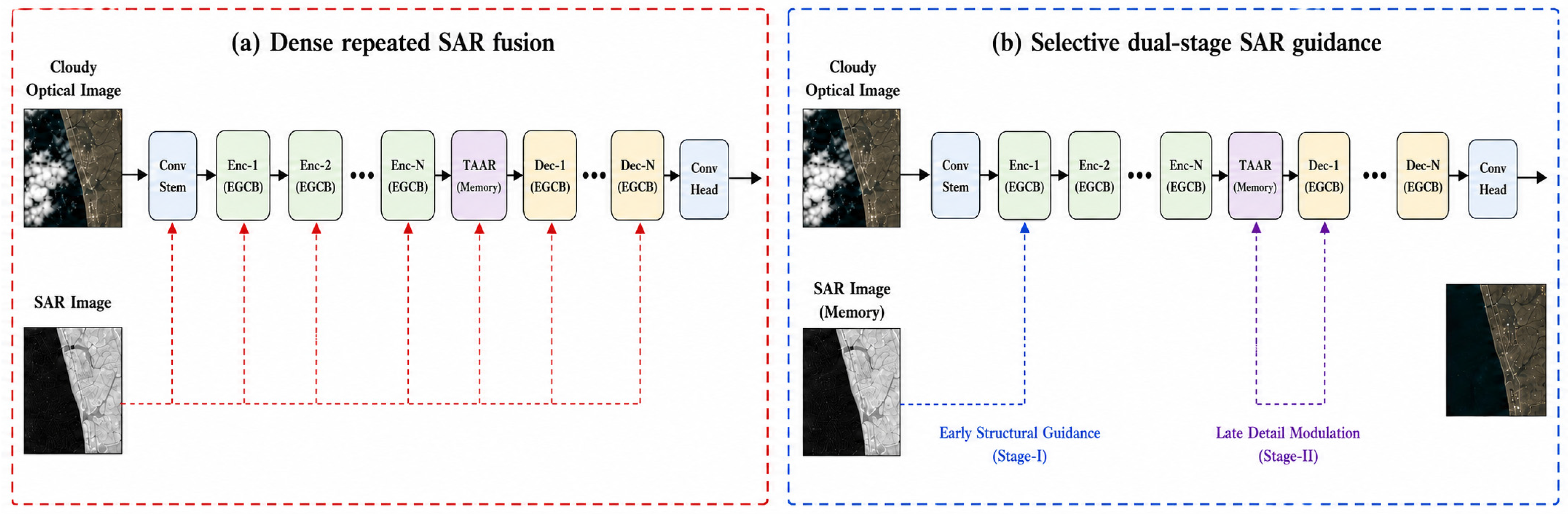
To address these issues, this paper proposes DST-SARNet, a dual-stage SAR-guided structural-texture restoration network for optical remote sensing cloud removal. Rather than repeatedly injecting SAR features into every restoration layer, DST-SARNet organizes SAR information according to its role in reconstruction. The SAR Structural Skeleton Generator (SSG) first converts SAR observations into stable geometric cues that constrain the optical reconstruction stream. The Efficient Global Context Block (EGCB) then models long-range spatial and channel relationships with reduced complexity. At the bottleneck, Texture-Aware Asymmetric Retrieval (TAAR) uses optical features as queries to read scene-matched texture contexts from SAR structural memory. Finally, Late SAR-Guided Spatial Modulation (LSGM) supplements high-frequency structural details before image reconstruction. In this design, dual stage refers to SSG and LSGM as the two explicit SAR guidance stages, while TAAR functions as an intermediate read-only memory retrieval operation rather than as a third dense SAR injection stage.

The three core modules form a clear functional sequence. EGCB provides efficient global context modeling for large cloud-covered regions; TAAR compensates for local texture and boundary attenuation caused by compressed attention; and LSGM restores high-frequency details near the output. This sequence improves thick-cloud restoration through explicit information division rather than through larger parameter scales or denser cross-modal concatenation.

The main contributions of this paper are summarized as follows.

(1) A dual-stage SAR-guided cloud removal framework is proposed. To address the limitation that dense SAR–optical fusion can propagate useful structures and modality-specific perturbations simultaneously, DST-SARNet organizes SAR information into two controlled guidance paths: early structural skeleton guidance and late high-frequency modulation. SAR therefore contributes as structural priors and detail compensation signals rather than as a generic auxiliary channel repeatedly propagated through the network.

(2) A structure–appearance decoupling strategy is proposed for SAR-assisted optical reconstruction. SSG extracts geometrically meaningful structural skeletons from SAR imagery, allowing the optical branch to recover color, semantics, and multispectral residuals under structural constraints, thereby reducing reconstruction uncertainty when both structural and spectral information are missing in thick-cloud regions.

(3) Two structural compensation modules, TAAR and LSGM, are designed. TAAR uses optical features as queries and SAR structural memory as keys and values to achieve optical-semantic-controlled structural retrieval. LSGM compensates high-frequency boundaries and texture details at the decoder end, thereby alleviating local detail attenuation caused by efficient attention compression.

(4) Experiments are conducted to evaluate reconstruction quality, computational efficiency, and convergence behavior. Comparisons with GAN-based, residual CNN-based, Transformer-based, and diffusion-related baselines on SMILE-CR and SEN12MS-CR, together with ablation studies, efficiency analysis, and training curves, demonstrate the contributions of efficient global context modeling and selective SAR structural guidance to thick-cloud restoration.

2. Materials and Methods

DST-SARNet is formulated as a SAR-assisted optical reconstruction network in which the optical branch remains the main reconstruction stream. SAR information is not treated as a generic auxiliary input throughout the network; instead, it is transformed into controlled structural cues with distinct functions. The network contains four key modules: SAR Structural Skeleton Generator (SSG), Efficient Global Context Block (EGCB), Texture-Aware Asymmetric Retrieval (TAAR), and Late SAR-Guided Spatial Modulation (LSGM). SSG produces early geometric constraints from SAR imagery; EGCB provides efficient global context modeling for the optical backbone; TAAR retrieves SAR structural memory according to optical semantics at the bottleneck; and LSGM compensates high-frequency boundaries and texture details near the output. Thus, dual stage refers to the two explicit SAR guidance stages, SSG and LSGM, while TAAR serves as an intermediate memory retrieval operation.

Cloud-contaminated optical degradation is not merely local texture blur. Thick clouds obscure surface boundaries, disrupt local textures, weaken large-scale color consistency, and change multispectral responses. CNN-based methods model local patterns effectively but are limited in global semantic and color-consistency modeling. Standard Transformers capture long-range dependencies but require high computation and memory for high-resolution remote sensing imagery [23,24,25,26]. DST-SARNet therefore uses EGCB to model spatial dependencies and channel interactions through shared projection and token compression. Because such compression may attenuate high-frequency details, SSG, TAAR, and LSGM provide structural compensation at the input side, bottleneck, and output side, respectively, making global modeling efficiency and detail restoration complementary.

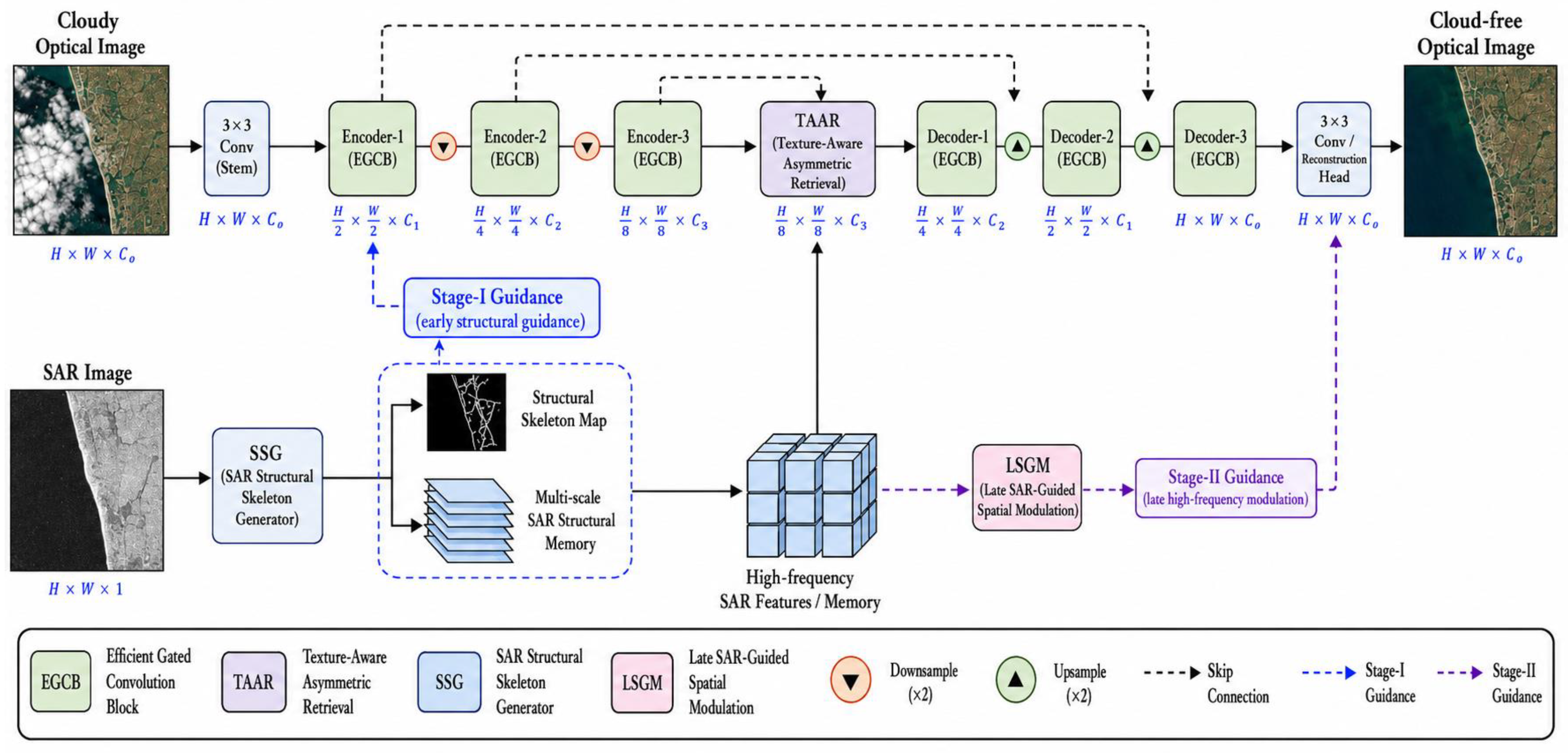
Figure 1 illustrates the overall architecture. DST-SARNet follows a Transformer-style encoder–bottleneck–decoder structure. SAR information is first converted into structural skeletons and multi-scale memory by SSG. The EGCB backbone then restores long-range spatial semantics and color consistency in the optical stream. At the bottleneck, TAAR uses optical semantic queries to selectively read same-scale SAR structural memory. Near the output, LSGM supplements high-frequency textures and boundary details. This design separates two questions that are often coupled in dense fusion: where SAR should guide the optical stream, and how SAR memory should be retrieved.

• Structural guidance feature extraction: Given a cloudy optical image and the corresponding SAR image, Stage-I SSG extracts a single-channel SAR structural skeleton and injects it into the optical branch as a geometric constraint. It first extracts relatively stable boundaries, texture directions, and local topological cues from SAR, and then generates early features through a shallow convolutional stem, avoiding nonselective diffusion of raw SAR intensity into multi-layer optical features.
• Multi-level global context encoding: The initial features are fed into a Transformer-style encoder composed of EGCBs. EGCB models spatial and channel relationships simultaneously and reduces the computational cost of standard self-attention through shared projection and compressed spatial key–value tokens. The encoder progressively reduces spatial resolution and increases channel depth, producing representations that integrate local texture, global semantics, and cross-channel consistency.
• SAR structural memory retrieval: At the bottleneck, TAAR uses deep optical features as queries to retrieve texture and contour information from the multi-scale SAR structural memory generated by SSG. SAR participates only as keys and values, while optical features remain the main reconstruction stream. The module therefore exploits the structural advantages of SAR while reducing excessive dominance of SAR features over the optical reconstruction path.
• High-quality residual image output: The decoder restores high-resolution features through skip connections. Before final reconstruction, LSGM uses high-frequency SAR structures to generate spatial scale and shift parameters for the late modulation of decoder features. This second explicit SAR-guidance stage is placed at the detail-sensitive position closest to the output. The reconstruction head then predicts residual information, which is added to the cloudy optical input to obtain the cloud-free prediction.

2.1. Problem Formulation and Structure–Appearance Decoupling

Given a cloudy optical image $X_c$, the corresponding SAR image $X_s$, and the cloud-free reference image $Y$, SAR-assisted optical cloud removal can be formulated as learning a mapping function that generates a prediction $\widehat{Y}$ whose spatial structure, pixel intensity, and spectral response are close to those of $Y$. In this setting, $X_c\in {\mathbb{R}}^{H\times W\times C_o}$ denotes the cloudy optical input, $X_s\in {\mathbb{R}}^{H\times W\times C_s}$ denotes the SAR input, and $Y\in {\mathbb{R}}^{H\times W\times C_y}$ denotes the target cloud-free optical image. $H$ and $W$ denote image height and width, while $C_o$, $C_s$, and $C_y$ denote the numbers of optical input channels, SAR channels, and target optical channels, respectively.

$$\widehat{\mathrm{Y}}={\mathrm{G}}_{\mathsf{\theta }}\left(\mathrm{A}\left({\mathrm{X}}_{\mathrm{c}}\right),{\mathrm{X}}_{\mathrm{s}}\right)$$

(1)

The mapping in Equation (1) defines the optical-dominant prediction process. Here, $\widehat{Y}$ is the predicted cloud-free image, $G_{\theta }\left(\cdot \right)$ represents the overall DST-SARNet mapping function, $\theta$ denotes the learnable parameters, and $A\left(\cdot \right)$ is the dataset-adaptive input adapter. The adapter is used only to handle input-channel differences across datasets and does not change the design principle that optical reconstruction remains the main branch while SAR provides structural priors.

The core difficulty in thick-cloud regions is that surface boundaries, texture directions, and spectral responses in optical imagery are often simultaneously missing. If only cloudy optical imagery is used, the network must infer both cloud-hidden structures and surface appearance, making the reconstruction space highly uncertain. SAR cannot directly provide true optical colors, but it can preserve structural cues such as roads, water boundaries, farmland textures, building outlines, and terrain scattering patterns. Therefore, this paper decomposes the restoration process into two complementary objectives: structural constraint and optical appearance reconstruction.

$${\mathrm{B}}_{\mathrm{s}}={\mathrm{S}}_{\mathsf{\varphi }}\left({\mathrm{X}}_{\mathrm{s}}\right)$$

(2)

$$\widehat{\mathrm{Y}}={\mathrm{R}}_{\mathsf{\theta }}\left(\mathrm{A}\left({\mathrm{X}}_{\mathrm{c}}\right),{\mathrm{B}}_{\mathrm{s}}\right)$$

(3)

Equations (2) and (3) implement this separation between structural guidance and optical appearance recovery. The function $S_{\varphi }\left(\cdot \right)$, parameterized by $\varphi$, extracts the SAR structural skeleton $B_s$, whereas $R_{\theta }\left(\cdot \right)$ denotes the optical-dominant reconstruction function. Accordingly, $B_s$ is not used for full spectral generation; it constrains cloud-hidden geometry so that the backbone can focus on color, semantics, and multispectral residual recovery.

From the perspective of conditional uncertainty, the SAR structural skeleton narrows the feasible reconstruction space in thick-cloud regions. Given a cloudy optical image, multiple interpretations of the hidden surface may be possible. After the SAR skeleton is introduced, boundary locations, texture directions, and spatial topology are constrained, and the restoration task becomes closer to optical appearance regression under structural conditions. This relationship can be described by the change in conditional entropy.

$$\mathcal{H}\left(\mathrm{Y}\mid {\mathrm{X}}_{\mathrm{c}},{\mathrm{B}}_{\mathrm{s}}\right)\le \mathcal{H}\left(\mathrm{Y}\mid {\mathrm{X}}_{\mathrm{c}}\right)$$

(4)

The entropy relation in Equation (4) expresses the same motivation from the perspective of reconstruction uncertainty. $H\left(\cdot \right)$ denotes conditional entropy, and the inequality indicates that introducing $B_s$ can reduce the uncertainty of reconstructing the target image under the cloudy optical condition $X_c$. This does not imply that SAR can replace optical reflectance; instead, SAR is used for structural inference and high-frequency compensation, while the optical branch remains responsible for color, semantics, and spectral appearance recovery.

2.2. Selective SAR Usage as a Perturbation-Controlled Design Rationale

The key issue in SAR-assisted cloud removal is not only whether SAR is used. It is also where SAR enters the network and in what form it is represented. SAR observations contain useful structural cues, such as boundaries, texture directions, and local topology. They also contain non-ideal components, including speckle noise, backscatter fluctuations, local geometric distortions, and residual SAR–optical registration errors.

Dense multi-layer fusion can repeatedly provide structural hints to the optical backbone. At the same time, it creates more opportunities for SAR-specific perturbations to enter deep feature propagation paths. When similar SAR evidence is injected at many layers, structural information may become redundant. Modality-specific perturbations can still propagate through different network paths and affect the reconstruction.

DST-SARNet adopts a perturbation-controlled selective usage strategy. Stage-I SSG first converts raw SAR observations into structural skeletons and multi-scale structural memory before they enter the optical restoration stream. TAAR then reads this stored memory at the bottleneck under the control of optical semantic queries. Stage-II LSGM finally uses high-frequency SAR features near the output stage, where detail compensation is most sensitive.

Accordingly, DST-SARNet does not stabilize SAR-assisted reconstruction by simply suppressing SAR information. Instead, it assigns SAR to stages where its structural evidence is most informative: early skeleton extraction for geometric constraints, bottleneck memory retrieval for semantic matching, and late modulation for detail compensation. This stage-specific allocation reduces redundant cross-modal propagation while retaining cloud-penetrating structural cues, and its effect is examined through ablation and module-replacement experiments.

2.3. Stage-I SAR Structural Skeleton Generator

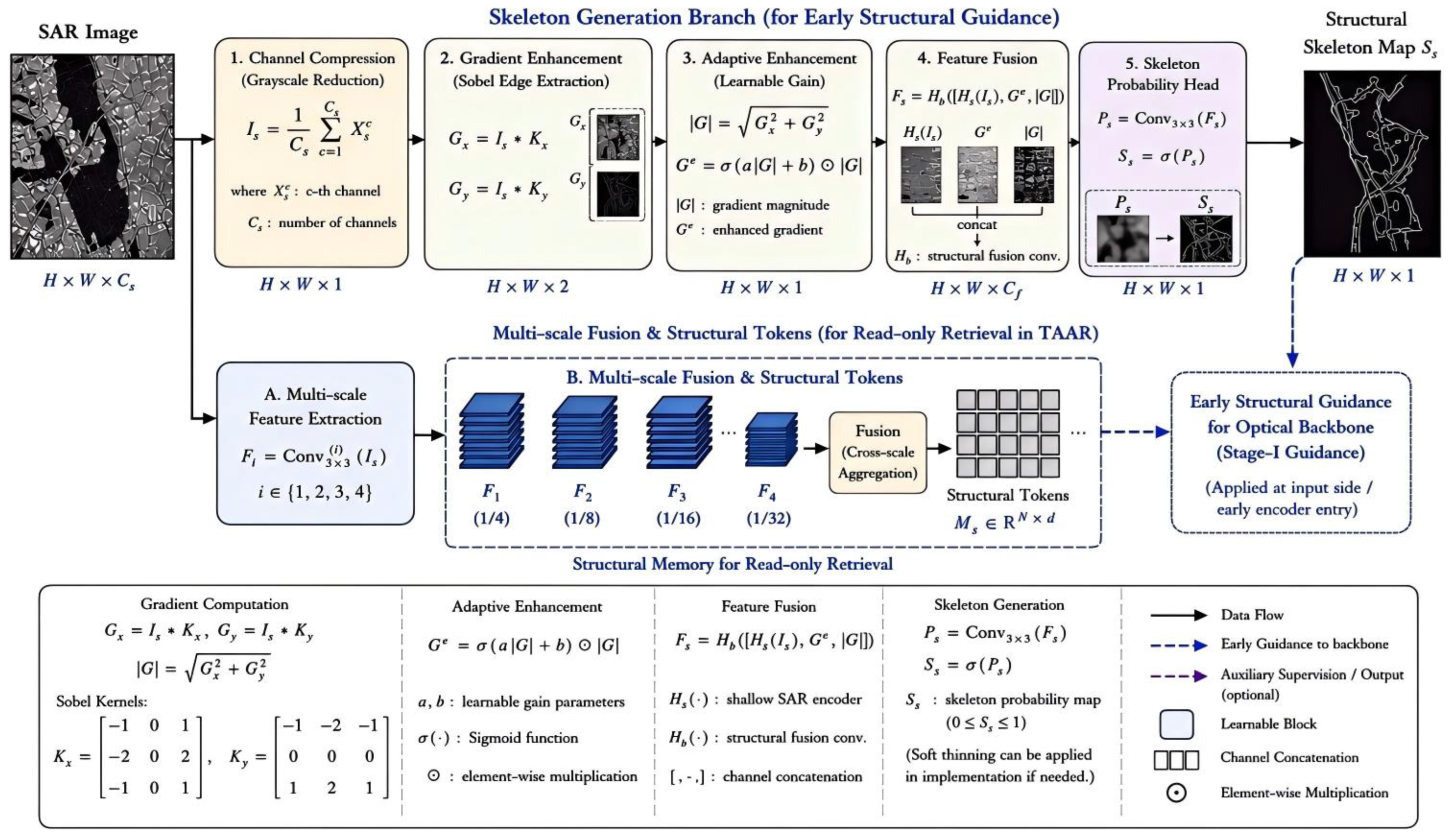
The Stage-I SAR Structural Skeleton Generator is shown in Figure 2. It converts SAR intensity observations into geometric priors for the optical backbone. Roads, water boundaries, ridges, farmland textures, and building outlines often appear in SAR imagery as local intensity discontinuities or directional textures. Directly concatenating raw SAR intensity with optical imagery forces the network to handle imaging-mechanism differences, speckle noise, and structural cues at the same time. DST-SARNet therefore structures SAR observations first. The resulting skeletons enter the optical reconstruction stream as more stable geometric cues.

For multi-channel SAR imagery, the module first performs channel compression to obtain a unified grayscale structural response:

$${\mathrm{I}}_{\mathrm{s}}={\displaystyle \frac{1}{{\mathrm{C}}_{\mathrm{s}}}}{\displaystyle \sum _{\mathrm{c}=1}^{{\mathrm{C}}_{\mathrm{s}}}}{\mathrm{X}}_{\mathrm{s}}^{\left(\mathrm{c}\right)}$$

(5)

Here, $I_s$ is the channel-compressed SAR structural response, $X_s^c$ is the $c$-th SAR channel, and $C_s$ is the number of SAR channels. For dual-polarization SAR, this channel-mean operation reduces scale differences between polarization channels and provides a stable response for subsequent gradient extraction.

Spatial gradients capture local boundary changes in SAR. After applying horizontal and vertical gradient kernels, the gradient responses are computed as follows:

$${\mathrm{G}}_{\mathrm{x}}={\mathrm{I}}_{\mathrm{s}}\ast {\mathrm{K}}_{\mathrm{x}} {\mathrm{G}}_{\mathrm{y}}={\mathrm{I}}_{\mathrm{s}}\ast {\mathrm{K}}_{\mathrm{y}}$$

(6)

The horizontal and vertical kernels $K_x$ and $K_y$ produce the gradient responses $G_x$ and $G_y$, respectively, where $\ast$ denotes convolution. These two directional responses are then combined to obtain the gradient magnitude:

$$\left|\mathrm{G}\right|=\sqrt{{\mathrm{G}}_{\mathrm{x}}^2+{\mathrm{G}}_{\mathrm{y}}^2+\mathsf{\epsilon }}$$

(7)

Magnitude G summarizes local SAR intensity discontinuities, and epsilon is used for numerical stability. Compared with raw SAR intensity, this gradient representation emphasizes structural discontinuities and is therefore more suitable for describing cloud-hidden contours.

Because SAR scattering intensity varies considerably across land-cover types, fixed gradient enhancement may overemphasize strong-scattering regions or ignore weak-texture regions. Therefore, a learnable gain is introduced to adaptively enhance the gradient response:

$${\mathrm{G}}^{\prime }=\mathsf{\sigma }\left(\mathsf{\alpha }\odot \left|\mathrm{G}\right|+\mathsf{\beta }\right)$$

(8)

The learnable coefficients $\alpha$ and $\beta$ control the strength and offset of the enhanced response $G^{\prime }$, while $\odot$ denotes element-wise multiplication and $\sigma \left(\cdot \right)$ denotes the Sigmoid function. This adaptive enhancement allows the network to adjust SAR structural responses from data rather than relying on fixed thresholds or hand-crafted enhancement rules.

The enhanced gradient and shallow SAR texture are fused to construct structural features:

$${\mathrm{P}}_{\mathrm{s}}={\mathrm{H}}_{\mathrm{b}}\left(\left[{\mathrm{I}}_{\mathrm{s}},{\mathrm{G}}^{\prime },\left|\mathrm{G}\right|,{\mathrm{F}}_{\mathrm{s}}\right]\right)$$

(9)

The shallow SAR encoder $H_s\left(\cdot \right)$ produces the texture feature $F_s$. The notation $\left[\cdot ,\cdot \right]$ represents channel concatenation, $H_b\left(\cdot \right)$ is the structural fusion convolution, and $P_s$ denotes the intermediate response of the skeleton probability map. The structural skeleton prediction is then obtained as follows:

$${\mathrm{B}}_{\mathrm{s}}=\mathsf{\sigma }\left({\mathrm{P}}_{\mathrm{s}}\right)$$

(10)

The resulting skeleton map provides the final geometric prior for the optical branch. It does not perform spectral substitution; instead, it enters the optical backbone as a structural constraint. To support TAAR at the bottleneck, Stage-I further constructs a multi-scale structural memory set for read-only retrieval.

The multi-scale structural memory is denoted by $M_s^r$ at the $r$-th scale, where $R$ is the number of scales. These memories preserve boundary information, texture directions, and local topology at different resolutions, providing candidate contexts for subsequent texture retrieval.

2.4. Efficient Global Context Block

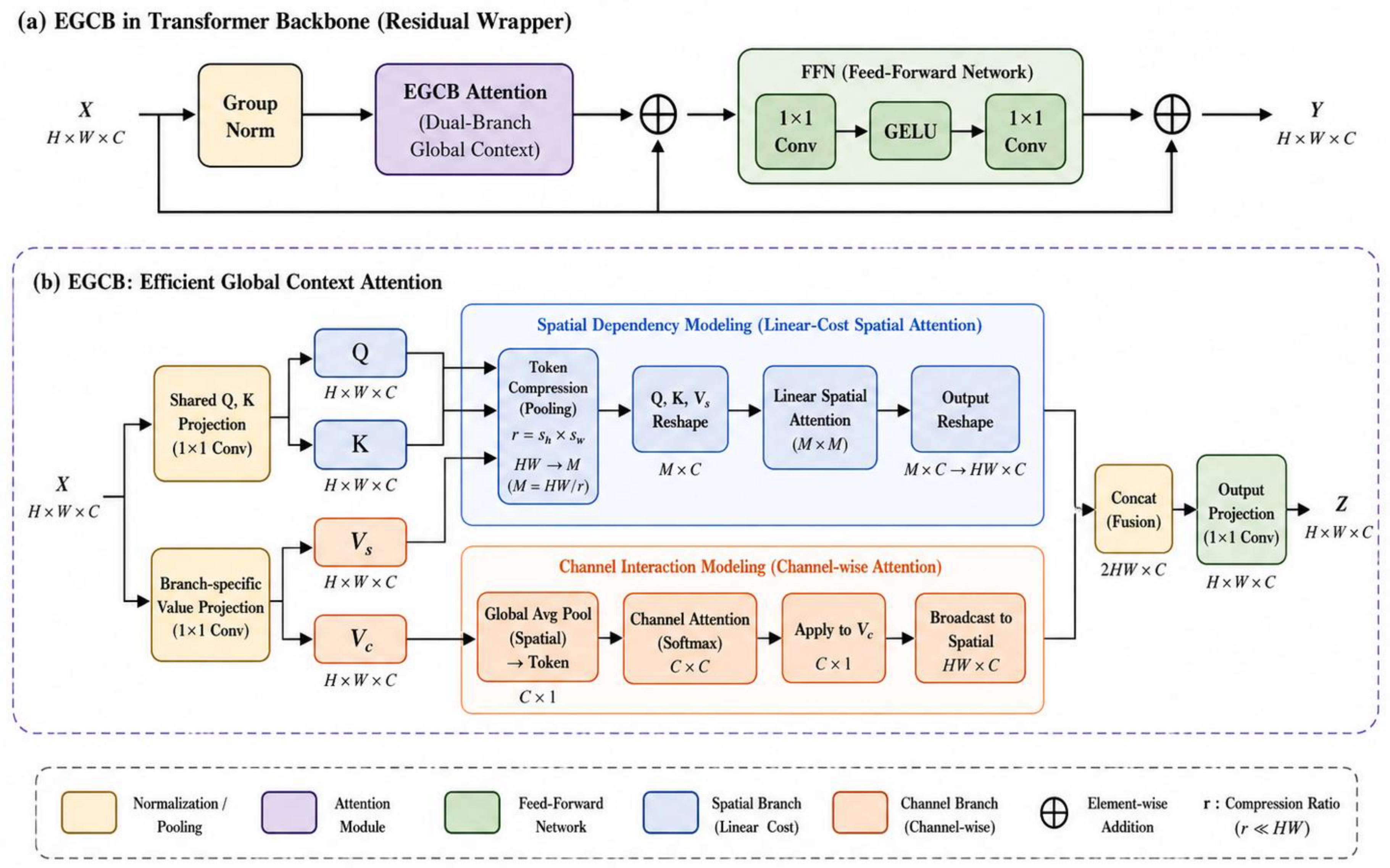
The Efficient Global Context Block (EGCB), shown in Figure 3, models long-range dependencies and channel relationships in large cloud-covered regions with reduced complexity. The module addresses two challenges: convolutional operations are limited in establishing long-distance semantic relationships inside large cloudy regions, and standard self-attention requires large spatial correlation matrices for high-resolution remote sensing images. EGCB decomposes global modeling into spatial dependency modeling and channel interaction modeling, and it shares query and key projections to reduce redundant mappings and improve spatial-channel representation consistency. This design preserves the global modeling advantage of Transformer-style architectures while avoiding the concentration of computational complexity in pairwise spatial-token correlations.

Given an input feature X, queries, keys, and values are obtained through normalization and 1 × 1 convolution:

$$\mathrm{Q}=\mathrm{X}{\mathrm{W}}_{\mathrm{Q}} \mathrm{K}=\mathrm{X}{\mathrm{W}}_{\mathrm{K}} \mathrm{V}=\mathrm{X}{\mathrm{W}}_{\mathrm{V}}$$

(11)

Here, $Q$, $K$, and $V$ are the query, key, and value features generated by the projection parameters $W_Q$, $W_K$, and $W_V$. EGCB shares the query and key projections between the spatial and channel branches, while retaining branch-specific value mappings. This design encourages the two branches to build compatible representations while learning complementary information.

The spatial dependency branch reduces the cost of spatial attention through token compression. Full spatial attention requires an N × N matrix, whereas EGCB compresses keys and values into M global anchors. In the implemented model, M is fixed as p = 64, corresponding to an 8 × 8 anchor grid:

$${\mathrm{K}}_{\mathrm{p}}=\mathrm{P}\left(\mathrm{K}\right) {\mathrm{V}}_{\mathrm{p}}=\mathrm{P}\left(\mathrm{V}\right)$$

(12)

The operator $P\left(\cdot \right)$ denotes adaptive pooling or token compression, and $K_p$ and $V_p$ are the compressed key and value tokens. With the default $p=64$ setting, full-resolution keys and values are summarized into an $8\times 8$ anchor grid before spatial attention is computed. The spatial attention output is then obtained by:

$${\mathrm{Z}}_{\mathrm{s}}=\mathrm{S}\mathrm{o}\mathrm{f}\mathrm{t}\mathrm{m}\mathrm{a}\mathrm{x}\left({\displaystyle \frac{\mathrm{Q}{\mathrm{K}}_{\mathrm{p}}^{\mathrm{T}}}{\sqrt{\mathrm{d}}}}\right){\mathrm{V}}_{\mathrm{p}}$$

(13)

The output $Z_s$ is the spatial dependency representation, and $d$ is the feature-dimension scaling factor. Under the fixed-anchor implementation, the attention map has size $N\times 64$ rather than $N\times N$, allowing long-range interaction through global anchors while avoiding full pairwise spatial correlation.

The channel interaction branch focuses on dependencies among multispectral bands and feature channels. Remote sensing cloud removal requires not only spatial texture restoration but also consistent responses among different spectral channels. The channel attention is written as:

$${\mathrm{Z}}_{\mathrm{c}}={\mathrm{V}}_{\mathrm{c}}\mathrm{S}\mathrm{o}\mathrm{f}\mathrm{t}\mathrm{m}\mathrm{a}\mathrm{x}\left({\displaystyle \frac{{\mathrm{Q}}^{\mathrm{T}}\mathrm{K}}{\sqrt{\mathrm{d}}}}\right)$$

(14)

The channel branch produces $Z_c$ by applying channel-wise attention to the value mapping $V_c$. This branch models dependencies among feature channels and multispectral responses, enabling the network to exploit complementary information across channels during cloud-contaminated reconstruction.

The outputs of the two branches are concatenated and projected for fusion:

The two branch outputs are then concatenated and projected, where $W_o$ is the output projection, $\left[Z_s,Z_c\right]$ denotes channel-wise concatenation, and $Z$ is the fused dual-branch attention representation. EGCB further uses a residual wrapper and a lightweight feed-forward network to improve training stability.

In this residual formulation, $\mathrm{G}\mathrm{N}\left(\cdot \right)$ denotes GroupNorm, $\mathrm{F}\mathrm{F}\mathrm{N}\left(\cdot \right)$ denotes a lightweight $1\times 1$ convolution-GELU-$1\times 1$ convolution feed-forward network, and $F_{\mathrm{o}\mathrm{u}\mathrm{t}}$ is the final EGCB output. Taking standard spatial self-attention as a reference, the computational cost of the spatial branch, channel branch, and their combination can be summarized as:

$${\mathcal{O}}_{\mathrm{E}\mathrm{G}\mathrm{C}\mathrm{B}}=\mathrm{O}\left(\mathrm{N}\mathrm{M}\mathrm{C}+\mathrm{N}{\mathrm{C}}^2\right)$$

(15)

The first term represents compressed spatial dependency modeling, and the second term represents channel interaction. Because the anchor number is fixed to M = p = 64, the spatial attention cost grows linearly with the number of spatial tokens N under a fixed anchor budget, whereas standard MHSA requires an N × N spatial correlation matrix. This explains why EGCB can be inserted at multiple encoder and decoder stages. The same compression may weaken fine-grained boundaries, so TAAR and LSGM are retained for subsequent structural detail compensation.

To make EGCB more reproducible, the concrete implementation is further specified here. Each EGCB receives a two-dimensional feature tensor $X\in {\mathbb{R}}^{B\times C\times H\times W}$, where $N=H\times W$ denotes the number of spatial tokens. In the implemented DST-SARNet configuration, the base channel dimension is 48, and the EGCB stages use 48, 96, and 192 channels at the high-, middle-, and bottleneck-resolution levels, respectively. The same fixed memory size $p=64$ is used for compressed spatial keys and values; therefore, adaptive average pooling compresses $K$ and $V$ into an $8\times 8$ anchor grid before spatial attention is computed.

The generator contains nine EGCBs: one at the 256 × 256 encoder level, two at the 128 × 128 encoder level, four at the 64 × 64 bottleneck level, and one in each decoder fusion stage after upsampling. This placement enables multi-resolution global context modeling while keeping the spatial attention map bounded by N × 64 rather than N × N.

The EGCB forward computation proceeds in five steps. First, GroupNorm is applied to the input feature, and a 1 × 1 convolution generates Q, K, and V with the same channel dimension C. Second, in the spatial branch, Q is reshaped to B × N × C, while K and V are pooled to B × C × 64 before the N × 64 attention map is computed. Third, in the channel branch, Q and K are normalized along the spatial dimension, and a C × C channel correlation matrix is computed to capture inter-channel dependencies. Fourth, the spatial and channel outputs are projected by branch-specific 1 × 1 convolutions, concatenated, and fused by another 1 × 1 convolution. Finally, both the fused attention output and the lightweight feed-forward network are wrapped by residual connections; the feed-forward network uses a 1 × 1 convolution-GELU-1 × 1 convolution structure with an expansion ratio of 2.0. The attention-fusion output projection and the final convolution of the feed-forward network are initialized to zero, so the block starts close to an identity mapping and becomes progressively active during training.

Unlike Restormer-style MDTA [27], which improves restoration efficiency mainly by computing attention along the channel dimension after local convolutional projection, EGCB explicitly retains two complementary paths: compressed spatial dependency modeling and channel interaction modeling. The spatial path uses compressed key–value anchors to preserve long-range spatial context for large cloud-covered regions, whereas the channel path models cross-channel dependencies that are important for multisource optical reconstruction. Unlike NAFNet-style restoration blocks [28], EGCB remains an attention-based global context module rather than an activation-free convolutional restoration block. Its role in DST-SARNet is therefore not limited to generic image restoration; it is embedded in a SAR-assisted restoration chain and paired with TAAR and LSGM to compensate for high-frequency detail attenuation caused by compressed global modeling, while leaving computational budget for structural memory retrieval and late SAR-guided detail compensation.

EGCB also differs from kernelized Linear Attention and Performer-style attention [37,38]. Linear Attention reduces quadratic token interaction by rewriting attention with kernel feature mappings, and Performer estimates softmax attention using random feature approximations. EGCB does not approximate the full softmax attention matrix in this manner. Instead, its spatial branch summarizes keys and values into a fixed set of global anchors, and its channel branch explicitly models inter-channel dependencies. This design is task-specific for SAR-assisted cloud removal: compressed spatial anchors provide affordable long-range context, channel interaction helps maintain multispectral consistency, and the saved computation is used for SAR structural retrieval and late SAR-guided detail compensation.

2.5. Texture-Aware Asymmetric Retrieval

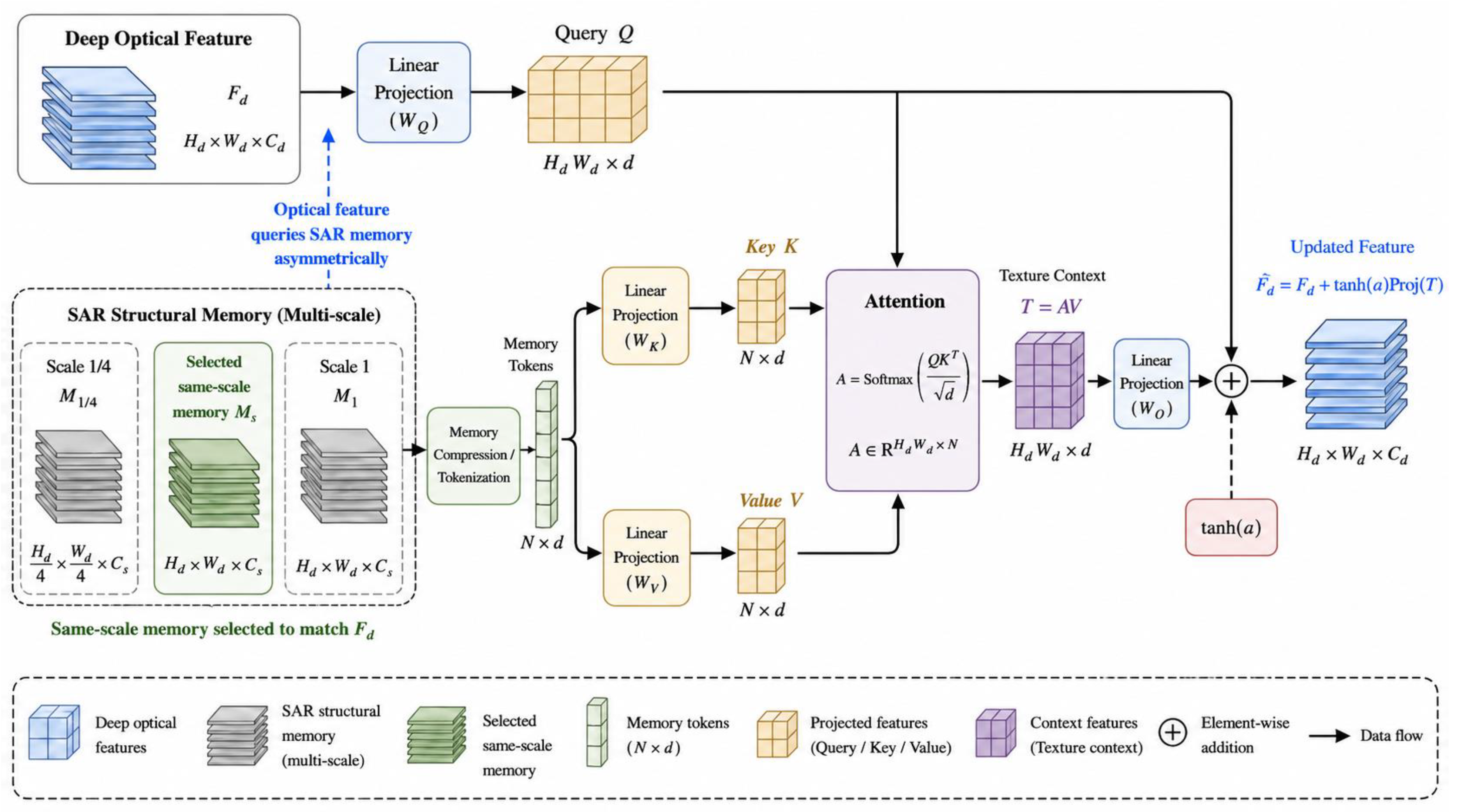
Texture-Aware Asymmetric Retrieval (TAAR), shown in Figure 4, reads texture context from SAR structural memory at the bottleneck. EGCB models global context with lower complexity, but token compression may weaken local boundaries and fine-grained texture responses. TAAR retrieves texture contexts that match the current optical semantics after the network has formed a global semantic representation. The module adopts an asymmetric design: deep optical features act as the query, while SAR structural memory provides the key and value. Optical features determine retrieval position and strength, and SAR exists only as readable structural memory. This design differs from symmetric dense fusion because SAR provides structural reference without replacing the optical reconstruction stream or continuously dominating feature propagation at every layer.

Let $F_d$ denote the bottleneck optical feature and $M_s^r$ the scale-matched SAR structural memory. TAAR first constructs the query, key, and value:

$${\mathrm{Q}}_{\mathrm{t}}={\mathrm{F}}_{\mathrm{d}}{\mathrm{W}}_{\mathrm{q}}$$

(16)

$${\mathrm{K}}_{\mathrm{t}}={\mathrm{M}}_{\mathrm{s}}^{\mathrm{r}}{\mathrm{W}}_{\mathrm{k}} {\mathrm{V}}_{\mathrm{t}}={\mathrm{M}}_{\mathrm{s}}^{\mathrm{r}}{\mathrm{W}}_{\mathrm{v}}$$

(17)

The two projections above define the asymmetric retrieval interface. $Q_t$ is the optical query, while $K_t$ and $V_t$ are SAR-derived keys and values obtained through $W_q$, $W_k$, and $W_v$. Because $Q_t$ comes from the bottleneck optical feature $F_d$, retrieval is dominated by current optical semantics; SAR memory provides structural context only when queried.

To reduce the cost of cross-attention, SAR structural memory is compressed into a fixed number of memory tokens by $P_m\left(\cdot \right)$. In the default DST-SARNet implementation, $P_m\left(\cdot \right)$ is realized by adaptive average pooling. Given a scale-matched SAR structural memory $M_s^r\in {\mathbb{R}}^{B\times C_s\times H_r\times W_r}$, the key and value projections first map it to the retrieval dimension $d$. The projected tensors are then pooled to an $8\times 8$ grid because the default setting uses $p_{\mathrm{t}\mathrm{o}\mathrm{k}\mathrm{e}\mathrm{n}\mathrm{s}}=64$. After flattening and transposition, the compressed key and value tensors are represented as $K_t,V_t\in {\mathbb{R}}^{B\times 64\times d}$. The optical query is reshaped as $Q_t\in {\mathbb{R}}^{B\times N_d\times d}$, where $N_d=H_d\times W_d$. The resulting attention map has size $N_d\times 64$, which avoids dense all-pixel SAR–optical attention while preserving read-only structural memory retrieval.

After compression, $K_t$ and $V_t$ are the 64-token SAR memory keys and values under the default configuration. Texture retrieval weights are obtained from the correlation between the optical query and these compressed SAR keys:

$${\mathrm{A}}_{\mathrm{t}}=\mathrm{S}\mathrm{o}\mathrm{f}\mathrm{t}\mathrm{m}\mathrm{a}\mathrm{x}\left({\displaystyle \frac{{\mathrm{Q}}_{\mathrm{t}}{\bar{\mathrm{K}}}_{\mathrm{t}}^{\mathrm{T}}}{\sqrt{\mathrm{d}}}}\right)$$

(18)

Attention weights $A_t$ measure the texture-retrieval affinity between optical queries and compressed SAR keys. The retrieved SAR texture context is then computed as:

$$\mathrm{T}={\mathrm{A}}_{\mathrm{t}}{\bar{\mathrm{V}}}_{\mathrm{t}}$$

(19)

The retrieved context T represents the SAR structural information most relevant to the current optical semantics. Rather than replacing or overwriting optical features, TAAR injects this context through a gated residual update:

$${\mathrm{F}}_{\mathrm{d}}^{\prime }={\mathrm{F}}_{\mathrm{d}}+\mathrm{t}\mathrm{a}\mathrm{n}\mathrm{h}\left(\mathsf{\alpha }\right){\mathrm{W}}_{\mathrm{o}}\left(\mathrm{T}\right)$$

(20)

In this update, $F_d^{\prime }$ is the refined bottleneck feature, $\alpha$ is a learnable gate, and $W_o\left(\cdot \right)$ projects the retrieved context back to the optical feature space. The factor $\mathrm{t}\mathrm{a}\mathrm{n}\mathrm{h}\left(\alpha \right)$ restricts the strength of SAR retrieval, preventing SAR noise or local misregistration from dominating early training. As a result, SAR participates as structural memory, whereas the optical branch remains responsible for color, semantics, and spectral appearance recovery.

TAAR differs from CRFormer-style multimodal fusion [9] and generic cross-attention designs in its asymmetric use of SAR. CRFormer focuses on multimodal Transformer fusion for cloud removal, whereas TAAR is a bottleneck-only structural memory retrieval unit inserted after optical semantic encoding rather than a complete multimodal fusion backbone. In standard cross-attention, the auxiliary modality may directly participate in feature updating and become an additional dominant reconstruction stream. In TAAR, the optical bottleneck feature always provides the query, and SAR only provides compressed structural keys and values. SAR is therefore used as read-only structural memory rather than as a symmetric fusion branch. The learnable gated residual further controls the retrieved SAR texture strength, reducing the risk that SAR speckle or local registration errors overwrite optical semantic features.

2.6. Late SAR-Guided Spatial Modulation

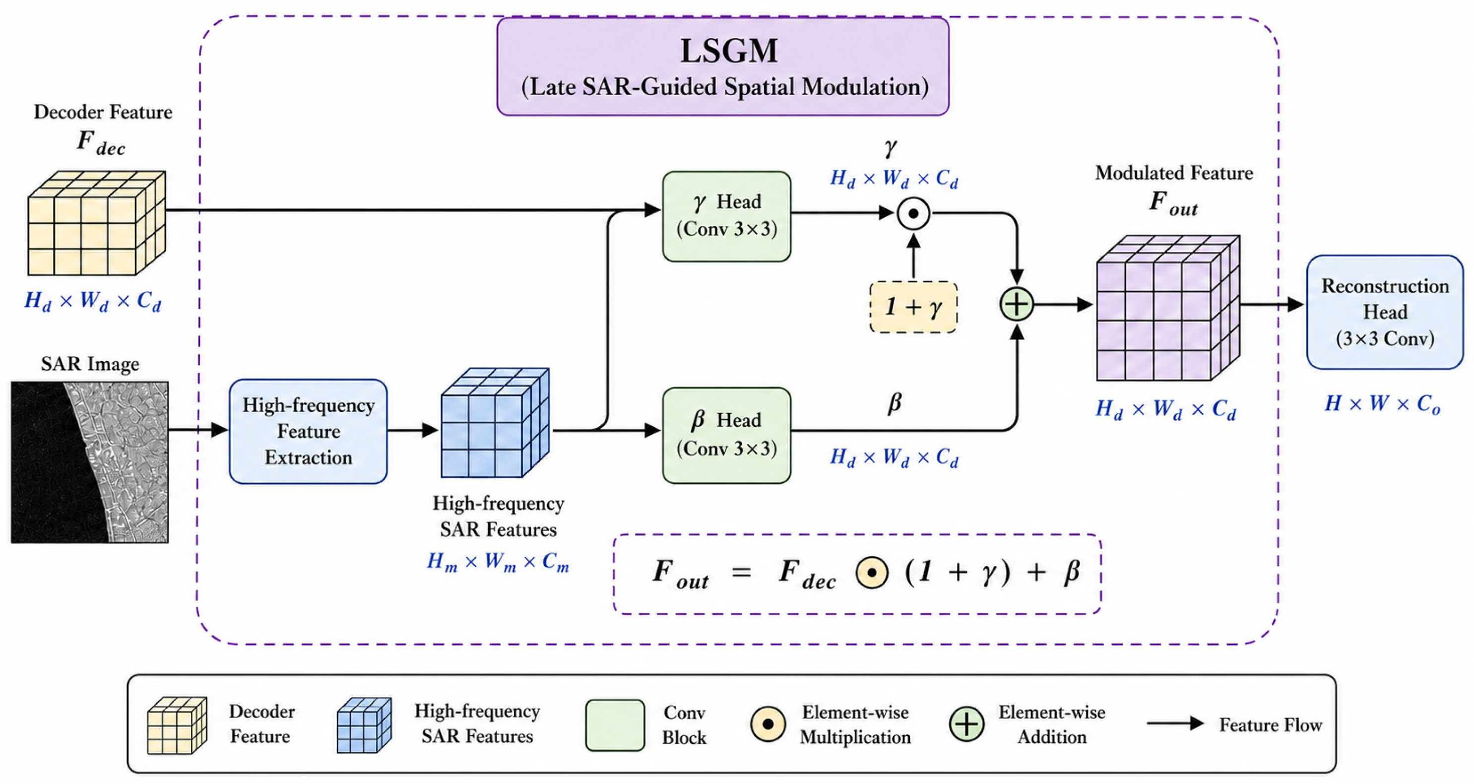
Late SAR-Guided Spatial Modulation (LSGM), shown in Figure 5, compensates for high-frequency structural details at the decoder end. The early SAR skeleton helps the backbone establish structural constraints, and TAAR reads structural memory at the bottleneck. Nevertheless, these cues may be smoothed after multiple encoding, attention compression, and decoding operations. The high-resolution stage before output is closest to the final image space and is the most detail-sensitive position for boundaries, roads, water edges, and building contours. DST-SARNet therefore performs the second explicit SAR-guidance stage at the decoder end, applying spatial modulation to decoder features so that SAR high-frequency information acts where detail compensation is most needed, rather than being repeatedly injected into every intermediate layer.

The SAR high-frequency branch extracts local structural cues from the original SAR image:

The feature $H_s$ is extracted by the lightweight high-frequency extractor $E_h\left(\cdot \right)$. This branch does not enter dense intermediate-layer fusion; instead, it is retained for detail compensation before output.

To match SAR high-frequency features with decoder features at the same spatial scale, an alignment mapping is first performed:

The aligned feature ${H_s}^{\prime }$ is obtained through the lightweight alignment module $A_h\left(\cdot \right)$. Based on this feature, LSGM generates spatially varying scale and bias parameters:

$$\mathsf{\gamma }=\mathsf{\tau }\mathrm{t}\mathrm{a}\mathrm{n}\mathrm{h}\left({\mathrm{W}}_{\mathsf{\gamma }}\left({\bar{\mathrm{H}}}_{\mathrm{s}}\right)\right)$$

(21)

The modulation heads $W_{\gamma }\left(\cdot \right)$ and $W_{\beta }\left(\cdot \right)$ predict the spatial scaling parameter $\gamma$ and bias parameter $\beta$, respectively. The coefficient $\tau$ controls the modulation amplitude, limiting excessive feature scaling and improving numerical stability near the decoder output.

Let $F_{\mathrm{d}\mathrm{e}\mathrm{c}}$ denote the final decoder feature. The late spatially modulated feature is defined as follows:

$${\mathrm{F}}_{\mathrm{o}\mathrm{u}\mathrm{t}}={\mathrm{F}}_{\mathrm{d}\mathrm{e}\mathrm{c}}\odot \left(1+\mathsf{\gamma }\right)+\mathsf{\beta }$$

(22)

The operator $\odot$ denotes element-wise multiplication. The term $1+\gamma$ preserves identity-mapping capability for compensating local structural offsets. This module supplements SAR high-frequency details before final output while avoiding repeated SAR injection at every decoder layer, thereby balancing structural sharpness and perturbation control.

LSGM is related to conditional modulation mechanisms such as FiLM [29] and SPADE [30], but it differs in condition source, modulation target, and physical role. FiLM usually performs feature-wise affine modulation using global or external conditions, whereas LSGM generates spatially varying modulation parameters from SAR high-frequency structures. SPADE performs spatially adaptive normalization using semantic layouts, whereas LSGM does not normalize the decoder feature distribution. Instead, it directly modulates late decoder features before residual reconstruction, supplementing SAR-guided high-frequency boundaries while preserving optical radiometric continuity. This design is well suited to cloud removal because reliable reflectance in non-cloud regions should be preserved, whereas cloud-hidden edges and textures should be selectively refined.

Overall, the relationship between the proposed modules and related mechanisms can be summarized as follows. EGCB is an efficient global context module for SAR-assisted restoration rather than a direct Restormer or NAFNet replacement. TAAR is an optical-query-driven SAR structural memory retrieval unit rather than symmetric multimodal fusion. LSGM is a Late SAR-Guided Spatial Modulation unit rather than a generic FiLM/SPADE normalization layer. These distinctions focus the method on the internal information flow of DST-SARNet: efficient global context modeling is followed by SAR structural memory retrieval and output-stage high-frequency compensation.

2.7. Residual Reconstruction and Training Objective

Remote sensing optical images often contain thick-cloud regions, thin-cloud regions, and unaffected regions simultaneously. Fully generating the entire image may damage reliable spectral information in unaffected areas. DST-SARNet adopts a residual reconstruction strategy so that the model focuses on learning correction terms for cloud-contaminated regions while preserving trustworthy observations in the input image:

In the residual prediction expression, $\mathit{\Delta }Y$ denotes the predicted residual, and $H_r\left(\cdot \right)$ is the reconstruction head. The final cloud-free prediction is:

$$\widehat{\mathrm{Y}}=\mathrm{C}\mathrm{l}\mathrm{i}\mathrm{p}\left({\mathrm{X}}_{\mathrm{b}\mathrm{a}\mathrm{s}\mathrm{e}}+\mathsf{\Delta }\mathrm{Y}\right)$$

(23)

Here, $X_{\mathrm{b}\mathrm{a}\mathrm{s}\mathrm{e}}$ is the cloudy optical input aligned with the output channels, and $\mathrm{C}\mathrm{l}\mathrm{i}\mathrm{p}\left(\cdot \right)$ constrains the prediction to the valid range. The residual form encourages the network to learn cloud-related corrections while reducing unnecessary changes in non-cloud regions.

The training objective consists of pixel reconstruction, structural preservation, edge consistency, spectral-angle constraint, range stability, and perceptual constraint terms:

$${\mathcal{L}}_{\mathrm{t}\mathrm{o}\mathrm{t}\mathrm{a}\mathrm{l}}={\mathsf{\lambda }}_{\mathrm{c}\mathrm{h}\mathrm{a}\mathrm{r}}{\mathcal{L}}_{\mathrm{c}\mathrm{h}\mathrm{a}\mathrm{r}}+{\mathsf{\lambda }}_{\mathrm{s}\mathrm{s}\mathrm{i}\mathrm{m}}{\mathcal{L}}_{\mathrm{s}\mathrm{s}\mathrm{i}\mathrm{m}}+{\mathsf{\lambda }}_{\mathrm{e}\mathrm{d}\mathrm{g}\mathrm{e}}{\mathcal{L}}_{\mathrm{e}\mathrm{d}\mathrm{g}\mathrm{e}}+{\mathsf{\lambda }}_{\mathrm{s}\mathrm{a}\mathrm{m}}{\mathcal{L}}_{\mathrm{s}\mathrm{a}\mathrm{m}}+{\mathsf{\lambda }}_{\mathrm{r}\mathrm{a}\mathrm{n}\mathrm{g}\mathrm{e}}{\mathcal{L}}_{\mathrm{r}\mathrm{a}\mathrm{n}\mathrm{g}\mathrm{e}}+{\mathsf{\lambda }}_{\mathrm{a}\mathrm{d}\mathrm{v}}{\mathcal{L}}_{\mathrm{a}\mathrm{d}\mathrm{v}}$$

(24)

The loss weights ${\lambda }_{\mathrm{c}\mathrm{h}\mathrm{a}\mathrm{r}}$, ${\lambda }_{\mathrm{s}\mathrm{s}\mathrm{i}\mathrm{m}}$, ${\lambda }_{\mathrm{e}\mathrm{d}\mathrm{g}\mathrm{e}}$, ${\lambda }_{\mathrm{s}\mathrm{a}\mathrm{m}}$, ${\lambda }_{\mathrm{r}\mathrm{a}\mathrm{n}\mathrm{g}\mathrm{e}}$, and ${\lambda }_{\mathrm{a}\mathrm{d}\mathrm{v}}$ balance the Charbonnier reconstruction loss, SSIM structural loss, edge-consistency loss, spectral-angle loss, range-stability loss, and adversarial perceptual loss, respectively. The reconstruction term constrains pixel fidelity, the structural term emphasizes local spatial consistency, the edge term strengthens texture-boundary responses, the spectral-angle term preserves multispectral response directions, the range term improves output numerical stability, and the adversarial term improves visual naturalness.

2.8. Dual-Stage SAR Guidance Versus Dense SAR Fusion

Figure 6 summarizes the difference between DST-SARNet and dense SAR fusion. Dense fusion methods tend to inject SAR features into multiple encoder and decoder layers. Such injection can provide structural hints across scales, but it also creates additional propagation paths for SAR speckle noise and cross-modal errors. DST-SARNet does not obtain stability by weakening SAR participation. Instead, it first converts SAR into structural skeletons and structural memory, and then uses this information through bottleneck retrieval and terminal modulation. In DST-SARNet, SAR is therefore not a repeatedly concatenated auxiliary channel but a source of structural priors, read-only memory, and high-frequency modulation signals.

The advantage of this design lies in its explicit information form. The Stage-I skeleton generator extracts cloud-hidden geometric cues and helps the optical backbone establish structural constraints. TAAR reads SAR structural memory at a deep semantic position so that structural supplementation is controlled by optical queries. LSGM compensates high-frequency boundaries before final output, placing detail enhancement at the position closest to the reconstructed result. Together, these components form a selective SAR-utilization chain in which the optical branch remains dominant for color, semantics, and spectral appearance, while the SAR branch focuses on structural cues and detail correction.

This mechanism is not a simple rejection of dense fusion. Dense fusion may still be effective when registration is reliable, noise is low, or additional denoising modules are available. This paper emphasizes that, in thick-cloud removal, the primary value of SAR lies in stable structural information rather than complete optical appearance. Restricting SAR to positions where structure is most needed and detail is most sensitive can preserve key surface textures while reducing perturbation propagation.

The essential difference between the dual-stage design and dense fusion lies in information form and propagation path. Dense fusion directly expands the participation range of SAR features in the network, which may amplify structural contributions and modality-specific perturbations simultaneously. DST-SARNet first converts SAR into a structural skeleton and then uses it in a controlled manner through bottleneck retrieval and terminal modulation, making SAR closer to a structural prior and a detail-compensation term. The optical main branch therefore remains responsible for color, semantics, and spectral appearance, while the SAR branch focuses on cloud-hidden structural cues and high-frequency boundary recovery.

3. Results

This section evaluates DST-SARNet for SAR-assisted optical remote sensing cloud removal. Experiments are conducted on two representative datasets. SMILE-CR is used for the main comparison and ablation experiments; its test samples contain cloud-contaminated imagery, SAR structural information, and cloud-free references under multisource observation conditions, making it suitable for evaluating reconstruction in truly cloud-obscured regions. SEN12MS-CR serves as an additional validation dataset. It contains Sentinel-2 cloudy images, Sentinel-2 cloud-free images, and Sentinel-1 SAR triplets, and is used to examine adaptability under 13-band multispectral reconstruction conditions.

The evaluation covers four aspects: reconstruction quality, visual effect, module contribution, and computational efficiency. Reconstruction quality is mainly measured by PSNR and SSIM, which reflect pixel fidelity and spatial structural similarity, respectively. SSIM is a widely used index for image structural similarity [39]. For SEN12MS-CR, SAM and MAE are additionally introduced to measure spectral-angle error and absolute reconstruction error between multispectral predictions and references. FID and LPIPS evaluate perceptual quality in RGB visualization space, providing auxiliary evidence for over-smoothing, texture distortion, and color shift from the perspectives of feature-distribution distance and deep perceptual feature distance [40,41]. Parameters, FLOPs, and FPS measure model complexity and inference efficiency. Because perceptual metrics depend on unified RGB projections or visualization space, they cannot fully replace 13-band spectral accuracy; therefore, conclusions on multispectral data are primarily based on PSNR, SSIM, SAM, and MAE.

All comparisons are performed with the same input resolution and a unified evaluation procedure. To avoid excessive reliance on overall averages that include weak-cloud or nearly cloud-free samples, the main quantitative evaluation on SMILE-CR focuses on 116 test samples with obvious cloud contamination, while thick-cloud analysis further uses 68 more challenging samples with stronger occlusion. This setting more directly reflects inference capability in real cloud-covered regions rather than only the ability to preserve unaffected input areas.

3.1. Experiment Design

3.1.1. Experimental Data

SMILE-CR is a multisource benchmark dataset for optical remote sensing cloud removal. It contains cloudy optical images, cloud-free reference images, and corresponding SAR observations, covering farmland, urban, mountainous, water, and vegetation scenes. Cloud contamination includes local thick clouds, large-area cloud occlusion, and thin-cloud interference, making the dataset suitable for evaluating structural recovery and texture reconstruction under optical information loss. The main quantitative evaluation uses 116 cloud-contaminated test samples, and the ablation analysis and visual comparison use 68 challenging thick-cloud samples to focus on recovery performance in truly cloud-obscured regions.

SEN12MS-CR contains cloudy Sentinel-2 images, cloud-free Sentinel-2 reference images, and Sentinel-1 SAR images. Sentinel-2 optical imagery consists of 13 bands, and Sentinel-1 SAR imagery includes VV and VH polarizations. This dataset is used to examine model stability under multispectral reconstruction and cross-sensor structural guidance. The winter subset is used for additional experiments, with a strict region-group split adopted to reduce spatial leakage among adjacent patches.

3.1.2. Methods of Comparison

Several representative remote sensing cloud removal methods are selected for comparison. Optical-only methods include Pix2Pix, SpA-GAN, AttentionGAN, and CRFormer, representing conditional image translation, adversarial generation, attention-enhanced generation, and Transformer-style optical restoration, respectively. SAR-assisted or generative methods include DSen2-CR, GLF-CR, DBD-CR, IDF-CR, and DiffCR, covering deep residual networks, global–local fusion, diffusion reconstruction, and latent-space restoration. The SEN12MS-CR experiments further include UnCRtainTS and other dataset-suitable baselines. These methods provide a broad comparison in terms of network structure, input modality, generation paradigm, and efficiency.

3.1.3. Experimental Environment and Parameter Settings

Experiments are performed on a server equipped with an NVIDIA GeForce RTX 3090 GPU with 24 GB of memory (NVIDIA Corporation, Santa Clara, CA, USA). The model is implemented in PyTorch 2.1.0+cu126 with CUDA 12.6 and Python 3.10.20 on a Linux x86_64 platform; the NVIDIA driver version was 595.71.05, and all reproduced experiments use the same hardware environment, spatial resolution, data preprocessing procedure, and evaluation metrics. For optical-only baselines, their original modality settings are retained. For SAR-assisted models, the input consists of cloudy optical imagery and the corresponding SAR imagery, and the output is cloud-free optical imagery. No test-set information is used during training. In SMILE-CR, cloud-contamination information is used only for regional statistics and sample screening during testing.

3.1.4. Quantitative Assessment Indicators

PSNR, SSIM, FID, LPIPS, model parameters, MACs, and FPS are used for comprehensive evaluation. PSNR measures pixel-level reconstruction accuracy, SSIM measures local structural similarity [39], FID evaluates the feature-distribution distance between generated results and cloud-free references [40], and LPIPS measures deep perceptual feature distance [41]. Parameters and MACs reflect model size and computational complexity, while FPS measures inference speed. For SEN12MS-CR, SAM and MAE are additionally reported; SAM measures the spectral-angle error of multispectral vectors, and MAE evaluates absolute reconstruction error. Because FID and LPIPS are usually computed from RGB projections or visualization space, they serve as auxiliary visual-quality evidence for 13-band data and cannot replace PSNR, SSIM, SAM, and MAE in multispectral reconstruction evaluation.

Unless otherwise stated, the upward arrow (↑) indicates that a higher value is better, whereas the downward arrow (↓) indicates that a lower value is better.

3.2. Computational Efficiency

Table 1. Quantitative evaluation of computational efficiency for different models.

Method	Params/M ↓	FPS ↑	FLOPs/G ↓
AttentionGAN	165.99	218.62	54.19
IDF-CR	75.11	67.37	69.55
Pix2Pix	57.18	733.04	18.14
DBD-CR	29.65	28.57	127.08
DiffCR	22.94	1.26	962.67
DSen2-CR	18.90	11.82	1238.16
CRFormer	17.18	39.17	56.72
GLF-CR	14.73	8.44	241.64
SpA-GAN	12.15	162.82	63.88
UnCRtainTS	0.56	168.64	2.98
DST-SARNet (Ours)	4.51	55.09	54.26

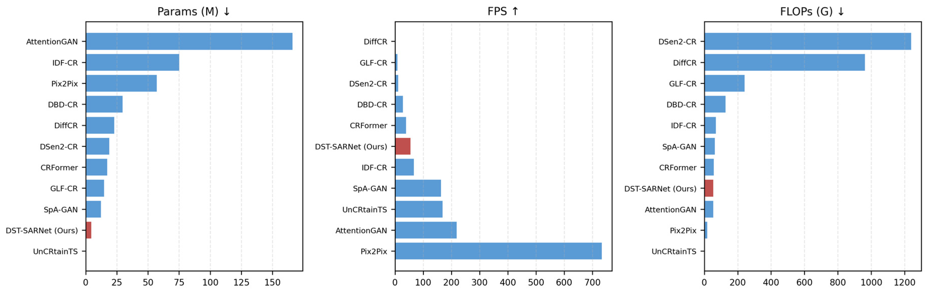
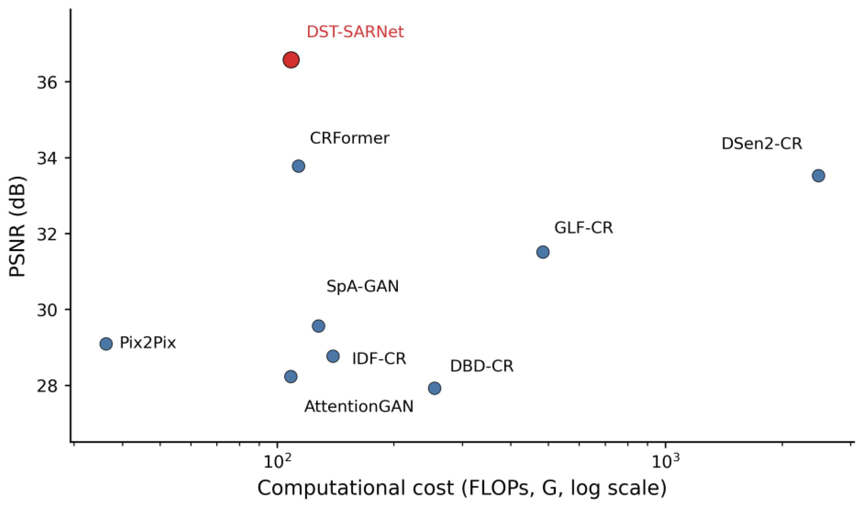
Note: FLOPs/G is obtained using a unified computation-statistics protocol and is used to characterize the relative computational complexity among different models. When the same method has slight implementation differences across datasets, the table reports representative statistics from the main comparison experiments.

reports model parameters, inference speed, and computational cost for different methods. It covers the main models involved in the experiments on both datasets, making it possible to compare DST-SARNet in terms of model scale and inference cost. Unlike comparisons based only on PSNR or SSIM, the efficiency table helps determine whether quality gains depend on large parameter counts or high computational cost.

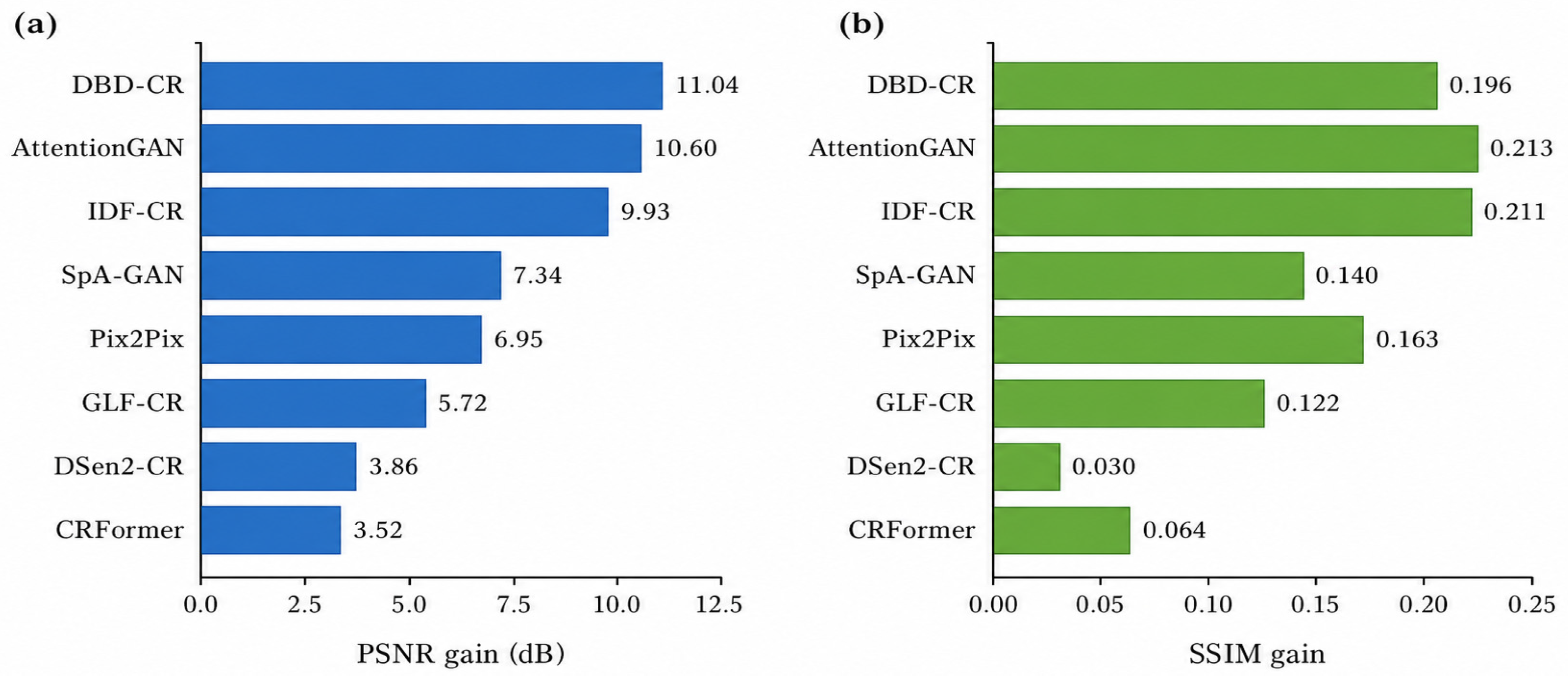
Table 1 shows that DST-SARNet has only 4.51 M parameters, substantially fewer than AttentionGAN, IDF-CR, Pix2Pix, DBD-CR, DiffCR, DSen2-CR, CRFormer, and GLF-CR. This result indicates that DST-SARNet improves performance mainly through structural-prior utilization and efficient global context modeling rather than through model-size expansion. Although UnCRtainTS and some lightweight GAN models have advantages in parameter count or FPS, they do not simultaneously maintain the highest reconstruction quality in subsequent metrics. Compared with CRFormer, DST-SARNet has fewer parameters with similar FLOPs and achieves higher PSNR, SSIM, and perceptual-quality scores on cloud-contaminated samples, indicating that selective SAR structural guidance is more suitable for thick-cloud removal than merely increasing global modeling capacity.

Pix2Pix and AttentionGAN have relatively high FPS, but both primarily operate as generative or adversarial mapping models and are prone to structural blurring and spectral shifts in thick-cloud regions. DSen2-CR and GLF-CR are representative SAR-assisted baselines that exploit SAR structural information, but the former has high computational cost, and the latter has low inference speed. DST-SARNet occupies a balanced position between quality and efficiency: the parameter count is significantly reduced, FLOPs remain moderate, and FPS is sufficient for single-pass inference. This behavior is consistent with the design objective of improving structural reconstruction in cloud-covered regions without diffusion-style multi-step sampling or large-scale dense fusion.

Figure 7 further visualizes the efficiency comparison in Table 1 by summarizing parameters, FPS, and FLOPs across representative methods.

3.3. Quantitative Evaluation

3.3.1. Quantitative Evaluation on SMILE-CR

Table 2. Quantitative evaluation of cloud removal quality on cloud-contaminated SMILE-CR test samples.

Method	PSNR/dB ↑	SSIM ↑	FID ↓	LPIPS ↓
DSen2-CR	33.5268	0.8683	122.8034	0.3039
CRFormer	33.7736	0.8455	151.8529	0.3829
GLF-CR	31.5147	0.8038	156.6910	0.4819
DBD-CR	30.4007	0.7749	143.1452	0.3807
SpA-GAN	29.5664	0.7898	147.7313	0.3966
Pix2Pix	29.0951	0.7627	196.3164	0.4500
IDF-CR	28.7706	0.7518	135.6019	0.3791
AttentionGAN	28.2349	0.7521	149.1633	0.3796
DST-SARNet (Ours)	36.5782	0.8891	106.8724	0.2205

presents quantitative results of different methods on the cloud-contaminated SMILE-CR test samples. PSNR and SSIM measure pixel and structural consistency between reconstructed images and cloud-free references, whereas FID and LPIPS evaluate visual perceptual quality. Compared with the full test set, this evaluation focuses more directly on cloud-contaminated samples and therefore better reflects restoration ability in cloud-covered regions.

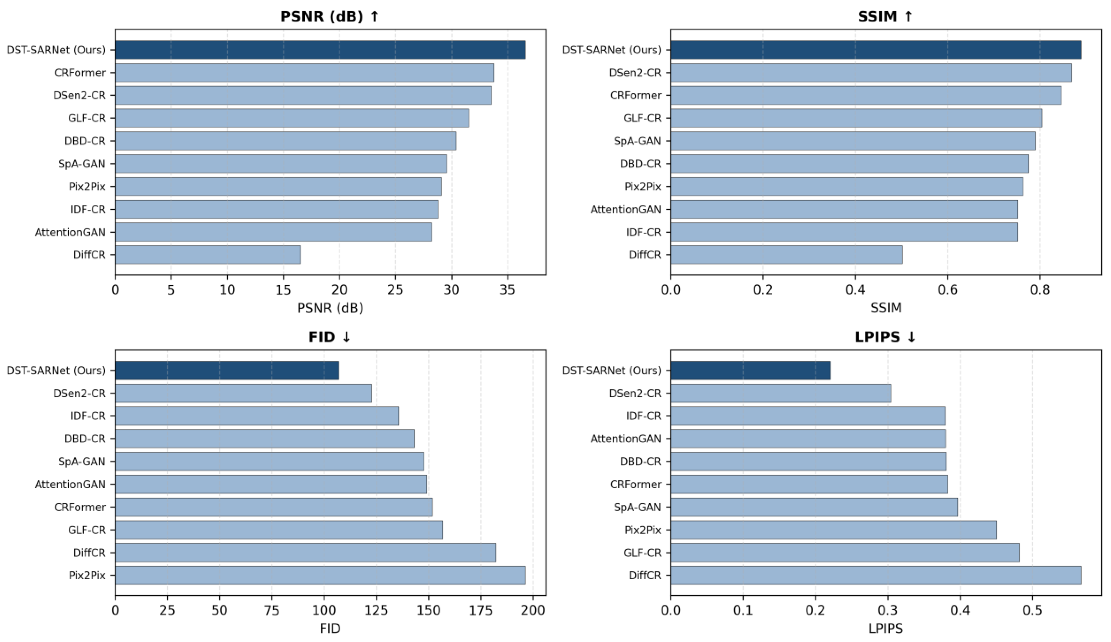
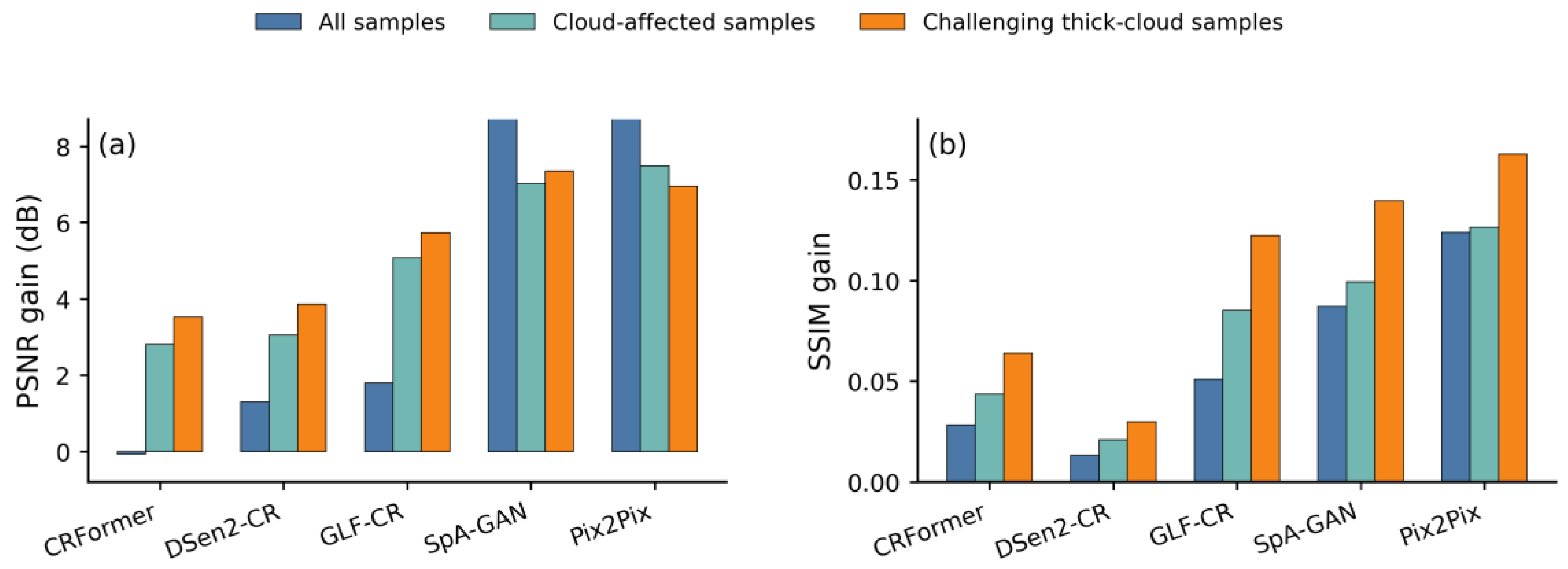
DST-SARNet achieves the highest PSNR and SSIM in Table 2, reaching 36.5782 dB and 0.8891, respectively. Compared with DSen2-CR, DST-SARNet improves PSNR by 3.0514 dB and SSIM by 0.0208. Compared with CRFormer, PSNR improves by 2.8046 dB and SSIM by 0.0436. The PSNR improvement indicates lower pixel reconstruction error in cloud-contaminated regions, and the SSIM improvement indicates better preservation of spatial structures such as roads, farmland boundaries, water edges, and urban textures.

For perceptual metrics, DST-SARNet obtains the lowest FID and LPIPS, 106.8724 and 0.2205, respectively. A lower FID indicates that predictions are closer to cloud-free references in overall visual distribution, while a lower LPIPS indicates higher consistency in deep perceptual feature space. By contrast, Pix2Pix has high inference speed but an FID of 196.3164 and an LPIPS of 0.4500, showing a large distribution gap between its generated results and real cloud-free imagery. CRFormer is close to strong baselines in pixel-level metrics, but its FID and LPIPS are much higher than those of DST-SARNet, indicating that optical-only global modeling is insufficient to restore local textures beneath thick clouds.

DSen2-CR performs strongly in SSIM, indicating that deep residual structures help maintain local spatial consistency. However, it has high computational costs and remains clearly weaker than DST-SARNet in FID and LPIPS. GLF-CR, as a SAR-assisted model, exploits SAR structural information to some extent, but is susceptible to SAR noise and cross-modal discrepancies in thick-cloud regions, resulting in degraded perceptual quality. DST-SARNet forms a controlled structural guidance chain through early SAR skeletons, bottleneck texture retrieval, and late spatial modulation, allowing SAR information to mainly act on cloud-hidden structures and high-frequency boundaries while the optical main branch restores color and semantics. Thus, it achieves balanced advantages across multiple metrics.

Figure 8 provides a bar-chart comparison of PSNR, SSIM, FID, and LPIPS on the cloud-contaminated SMILE-CR test samples, complementing the numerical results in Table 2. In Figure 8, the dark-blue bar denotes DST-SARNet (Ours), whereas the light-blue bars denote the competing methods.

3.3.2. Quantitative Evaluation on SEN12MS-CR

Table 3. Additional quantitative evaluation on cloud-contaminated SEN12MS-CR test samples.

Method	PSNR/dB ↑	SSIM ↑	SAM ↓	MAE ↓	FID ↓	LPIPS ↓
DiffCR	19.6753	0.6466	0.2333	0.0845	193.8251	0.4920
AttentionGAN	26.6871	0.7635	0.1764	0.0370	101.6616	0.3455
DSen2-CR	26.2992	0.7236	0.2066	0.0361	107.5798	0.3331
GLF-CR	26.8772	0.7818	0.1685	0.0346	116.1991	0.3542
SpA-GAN	26.6308	0.7585	0.1835	0.0345	205.2819	0.4668
UnCRtainTS	27.6080	0.7938	0.1785	0.0314	175.6998	0.4545
DST-SARNet (Ours)	27.6753	0.8046	0.1527	0.0325	103.0038	0.3451

provides additional quantitative results on the SEN12MS-CR winter data. This dataset contains 13-band cloudy and cloud-free Sentinel-2 imagery and dual-polarization Sentinel-1 VV/VH SAR imagery. Because the output target consists of 13-band multispectral imagery, SAM and MAE are important for this dataset. SAM measures the angular difference between predicted and reference spectral vectors and reflects the preservation of multispectral signatures; MAE reflects absolute pixel error and helps assess radiometric recovery stability across models.

DST-SARNet obtains the highest PSNR, highest SSIM, and lowest SAM on SEN12MS-CR, reaching 27.6753 dB, 0.8046, and 0.1527, respectively. This result indicates that the model recovers structures and textures not only in the RGB visualization space of SMILE-CR but also under Sentinel-2 multispectral conditions, while maintaining strong spatial structure and spectral-direction consistency. Compared with UnCRtainTS, DST-SARNet slightly improves PSNR, increases SSIM by 0.0108, and reduces SAM by 0.0258, indicating that SAR structural skeletons and late modulation remain effective for multispectral structural restoration.

The FID and LPIPS results on SEN12MS-CR should be interpreted in light of the characteristics of multispectral reconstruction. AttentionGAN achieves the lowest FID and DSen2-CR obtains the lowest LPIPS, while DST-SARNet remains close to the best performance in both perceptual metrics. Because FID and LPIPS are usually computed from RGB projections or visualization space, they are more suitable as auxiliary evidence for visual quality than as the sole basis for evaluating complete multispectral reconstruction quality. Considering PSNR, SSIM, SAM, and MAE together, DST-SARNet maintains strong structural and spectral recovery performance on this additional dataset.

3.4. Qualitative Evaluation on Thick-Cloud Samples

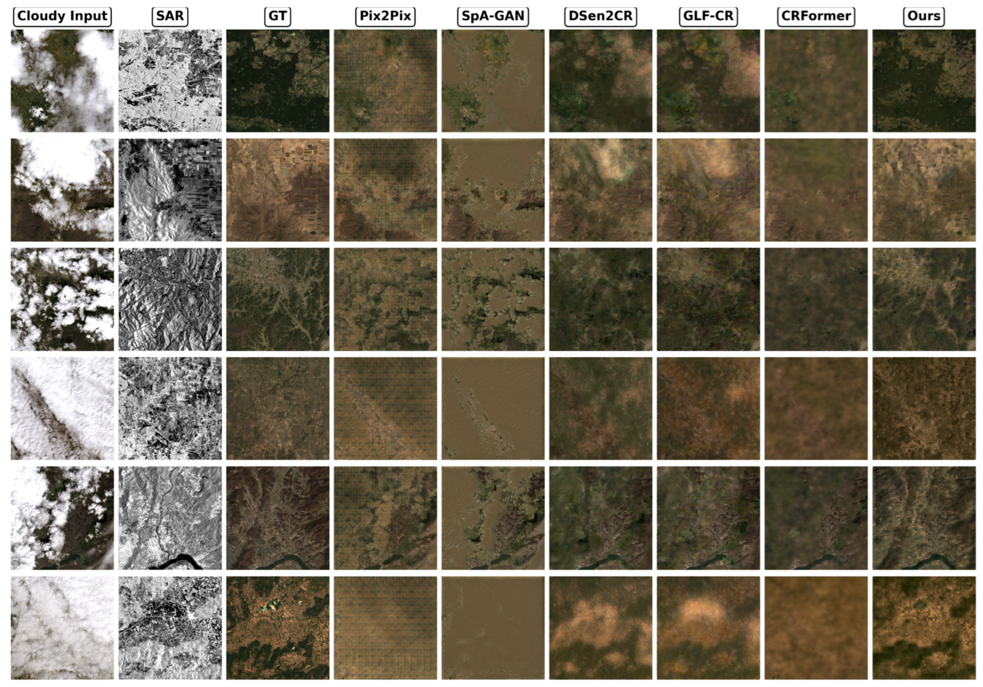
Figure 9 presents visual comparisons of multiple models on thick-cloud SMILE-CR samples. Compared with thin-cloud or weakly contaminated samples, the displayed examples contain larger cloud-covered areas, and the surface texture beneath the clouds is difficult to identify directly from the cloudy input. These examples are therefore more suitable for testing whether a model can recover cloud-hidden surface morphology using SAR structural information, rather than relying on extrapolation from visible regions or input copying.

As shown in Figure 9, Pix2Pix reduces the visual salience of white clouds in most samples, but the generated results usually contain blurred textures and grayish or yellowish global tones. This indicates that a simple conditional generation model can learn the global mapping from cloudy to cloud-free images but cannot accurately restore surface structures completely obscured by thick clouds. SpA-GAN generates relatively continuous surface colors in local regions, but roads, farmland boundaries, and mountainous textures beneath clouds remain weak, suggesting that its spatial attention is insufficient for stable structural inference when reliable optical information is missing.

DSen2-CR and GLF-CR use SAR information to assist cloud-hidden structural recovery, and their visual results are clearly better than those of purely generative models. Nevertheless, DSen2-CR still shows large-area smoothing in some samples, and GLF-CR presents noise enhancement or locally unnatural colors in some mountainous and river regions. CRFormer produces relatively stable overall colors, but local texture recovery remains insufficient, especially in high-frequency regions such as ridges, farmland parcels, and narrow roads where boundaries tend to be weakened. These observations are consistent with the quantitative results: global modeling or deep residual structures improve overall consistency, but explicit cloud-hidden structural priors are still needed for thick-cloud regions.

DST-SARNet shows clearer surface contours and more natural color transitions in Figure 9. For mountainous samples, the model better recovers continuous ridges and valley textures; for farmland and urban-edge samples, it preserves fine block textures and road structures; and for large-area thick-cloud samples, the output contains no obvious residual clouds or large pseudo-color patches. This advantage comes from selective dual-stage SAR utilization: Stage-I provides input-side structural skeletons, TAAR reads SAR structural memory at the bottleneck, and LSGM compensates high-frequency boundaries before output. These components jointly reduce detail loss caused by compressed attention while avoiding speckle diffusion caused by repeated SAR injection in intermediate layers.

3.5. Ablation Study

To verify the contribution of each component in DST-SARNet to thick-cloud removal, stepwise ablation experiments are conducted on challenging thick-cloud samples from SMILE-CR. These samples have stronger cloud occlusion and less directly usable surface information in the optical input, making them suitable for evaluating the effects of SAR structural priors, texture retrieval, and late spatial modulation under complex cloud contamination. The ablation study does not treat performance as a monotonic improvement across all metrics; instead, it analyzes each module from the perspectives of computational efficiency, pixel-level reconstruction quality, and perceptual quality.

In

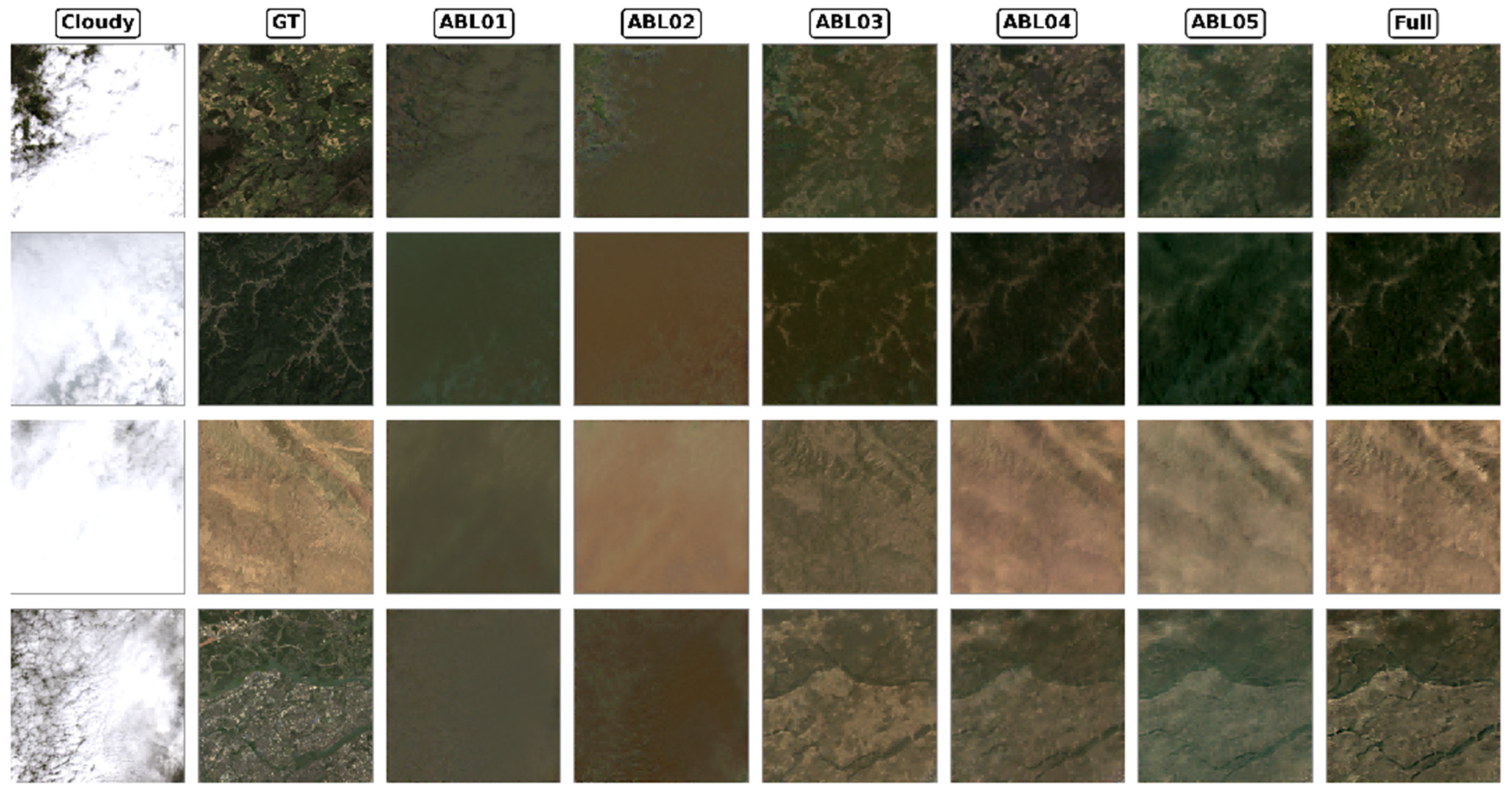
Table 4. Ablation results on challenging thick-cloud SMILE-CR samples.

Variant	PSNR ↑	SSIM ↑	MAE ↓	FID ↓	LPIPS ↓	Params (M) ↓	FLOPs (G) ↓	FPS ↑
ABL01	30.6036	0.7861	0.032416	111.6507	0.393940	2.6953	28.2361	50.6057
ABL02	29.9691	0.7797	0.033976	107.4842	0.392560	3.2367	37.0126	78.7599
ABL03	31.0929	0.8144	0.030731	89.6610	0.269638	3.3015	41.2311	69.8246
ABL04	33.4400	0.8453	0.017949	90.9458	0.248015	4.4291	48.7714	61.2208
ABL05	33.9061	0.8558	0.016909	93.0863	0.249978	4.5134	54.2638	55.1224
Full	33.7277	0.8432	0.017243	86.4348	0.194809	4.5134	54.2638	55.2004

Note: The best results are highlighted in bold. ABL01 denotes standard-MHSA optical-only; ABL02 denotes EGCB optical-only; ABL03 denotes EGCB + SSG; ABL04 denotes EGCB + SSG + TAAR/Fusion; ABL05 denotes EGCB + SSG + TAAR + LSGM, NoGAN; Full denotes the complete DST-SARNet.

, ABL01 denotes an optical-only baseline using standard multi-head self-attention without SAR imagery or EGCB. ABL02 replaces standard multi-head self-attention with EGCB while still using only optical input, verifying the influence of efficient global modeling on efficiency and reconstruction quality. ABL03 adds the SAR Structural Skeleton Generator to ABL02 and evaluates the effect of early SAR structural priors on restoring surface contours in thick-cloud regions. ABL04 further introduces the TAAR/Fusion mechanism, allowing deep optical features to retrieve texture contexts from SAR structural memory. ABL05 adds the LSGM late SAR spatial modulation module to ABL04 without adversarial loss, showing the influence of late SAR high-frequency compensation on pixel-level reconstruction. Full denotes the complete DST-SARNet model, which adds perceptual constraints and adversarial training terms to ABL05 to enhance texture naturalness and visual realism.

The comparison from ABL01 to ABL02 shows that EGCB mainly improves computational efficiency rather than directly improving thick-cloud reconstruction accuracy. Compared with ABL01, ABL02 slightly decreases PSNR and SSIM, whereas FPS increases from 50.6057 to 78.7599, indicating that efficient attention significantly reduces the cost of global modeling. This result also suggests that linearized or compressed attention alone is insufficient for detail restoration in thick-cloud regions: compressed global context improves long-range modeling efficiency but may weaken local boundaries and high-frequency texture responses. EGCB is therefore more suitable as an efficient backbone for subsequent SAR structural guidance modules than as a standalone solution for complete thick-cloud restoration.

The transition from ABL02 to ABL03 demonstrates the effectiveness of the SAR structural skeleton. After SSG is added, PSNR increases from 29.9691 to 31.0929, SSIM increases from 0.7797 to 0.8144, MAE decreases from 0.033976 to 0.030731, FID decreases from 107.4842 to 89.6610, and LPIPS decreases from 0.392560 to 0.269638. These changes show that cloud-hidden structural information provided by SAR improves geometric contour and spatial-structure recovery in thick-cloud regions. Compared with ABL02, which relies only on cloudy optical imagery, ABL03 yields clearer surface boundaries and more stable texture directions, confirming the necessity of Stage-I SSG in thick-cloud scenarios.

After TAAR/Fusion is introduced on the basis of ABL03, ABL04 further improves reconstruction quality. PSNR increases from 31.0929 to 33.4400, SSIM increases from 0.8144 to 0.8453, MAE decreases from 0.030731 to 0.017949, and LPIPS decreases from 0.269638 to 0.248015. This indicates that providing SAR skeletons only at the input side is insufficient for restoring complex textures beneath thick clouds; deep optical semantic features still need to retrieve scene-matched texture contexts from SAR structural memory. TAAR uses optical features as queries and SAR structural memory as keys and values, enabling SAR to participate as read-only memory. This design enhances structural compensation while reducing excessive interference from SAR features in the optical reconstruction stream.

ABL05 further introduces the LSGM late SAR spatial modulation module and obtains the highest PSNR, highest SSIM, and lowest MAE without adversarial loss. Its PSNR reaches 33.9061, SSIM reaches 0.8558, and MAE decreases to 0.016909, indicating that late SAR high-frequency modulation directly contributes to pixel-level restoration and edge consistency. This module generates spatial scale and shift parameters from SAR high-frequency features at the decoder end, compensating details such as roads, water boundaries, farmland textures, and building contours before final output. Compared with ABL04, the improvement in ABL05 shows that SAR information is useful not only as an early structural prior but also as high-frequency detail correction near the output stage.

Compared with ABL05, the Full model slightly decreases PSNR and SSIM, but LPIPS decreases further from 0.249978 to 0.194809, and FID decreases from 93.0863 to 86.4348. This indicates that the complete model does not simply maximize pixel-level metrics; rather, it balances pixel fidelity and perceptual quality. Adversarial constraints and perceptual terms guide generated results toward the texture distribution of real cloud-free imagery, which may slightly sacrifice strict pixel-wise consistency but substantially improve visual naturalness. This phenomenon is consistent with common observations in remote sensing image generation tasks: pixel losses are more favorable for PSNR and SSIM, whereas adversarial constraints are more beneficial for texture realism and perceptual consistency.

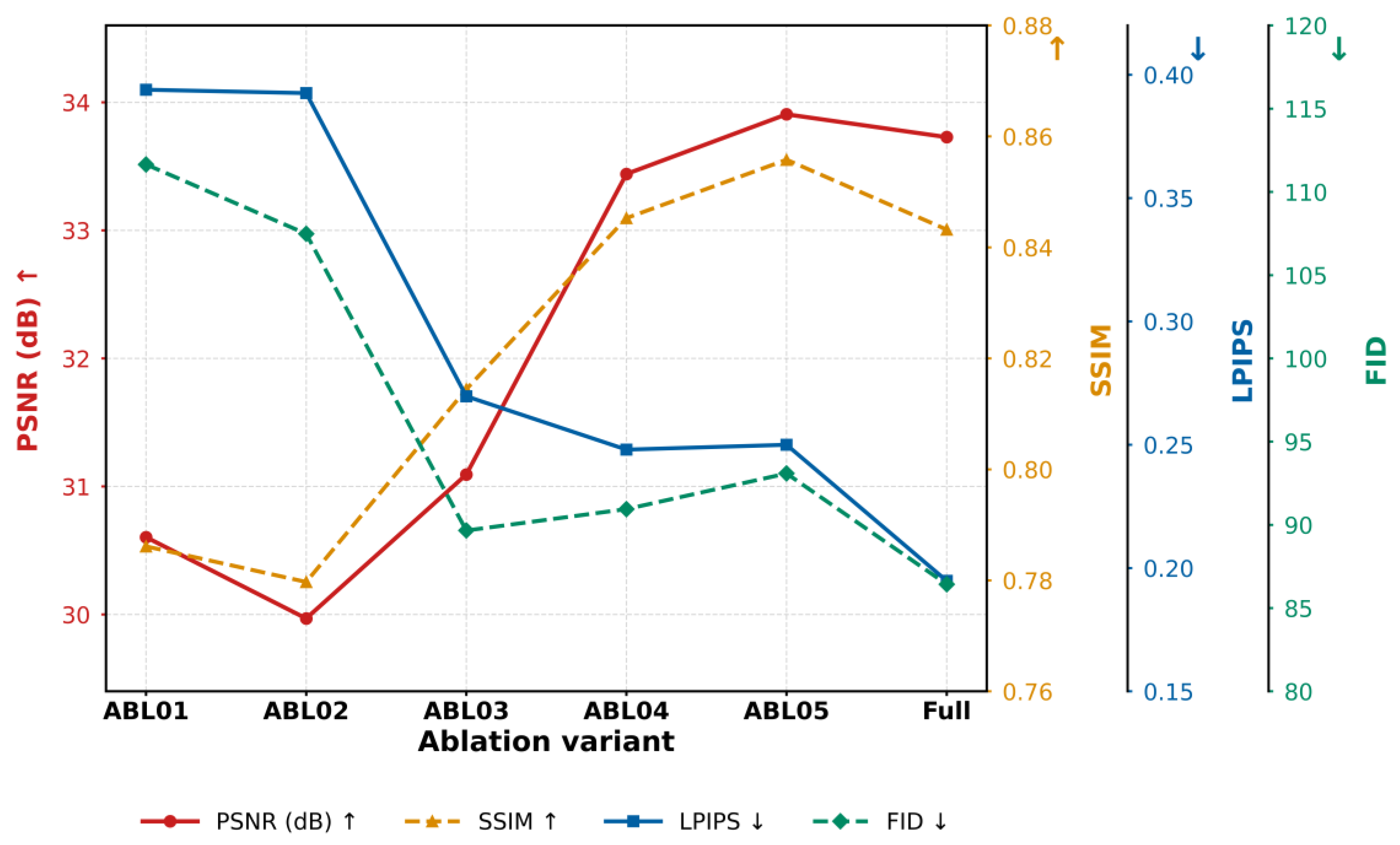
As shown in Table 4 and Figure 10, ABL02 slightly decreases PSNR and SSIM compared with ABL01, but FPS increases from 50.61 to 78.76. This indicates that EGCB mainly verifies the computational advantage of efficient attention rather than independently improving reconstruction accuracy. After SSG is introduced in ABL03, PSNR increases from 29.9691 to 31.0929, SSIM increases from 0.7797 to 0.8144, and LPIPS decreases from 0.3926 to 0.2696, showing that the early SAR structural skeleton significantly enhances geometric recovery in thick-cloud regions.

After TAAR/Fusion is introduced in ABL04, PSNR increases to 33.4400 and MAE decreases to 0.017949, indicating that asymmetric retrieval from SAR structural memory provides effective texture context for the optical main branch. After LSGM is added in ABL05, the model obtains the highest PSNR, highest SSIM, and lowest MAE, confirming the direct contribution of late SAR modulation to pixel-level structural fidelity. Compared with ABL05, the Full model slightly decreases PSNR and SSIM, but LPIPS decreases further from 0.2500 to 0.1948, suggesting that adversarial perceptual constraints benefit visual naturalness and texture-distribution approximation. Therefore, the advantage of the complete model should be understood as a trade-off between pixel fidelity and perceptual quality rather than as a mechanical monotonic improvement across all metrics.

Figure 11 shows the effects of different ablation variants on thick-cloud samples. ABL01 and ABL02 mainly rely on cloudy optical context for restoration, and their results are prone to large-area smoothing, color shift, and structural loss. After the SAR structural skeleton is introduced in ABL03, cloud-hidden surface contours and texture directions become clearer. ABL04 and ABL05 further improve mountainous textures, farmland boundaries, and local surface details. The Full model exhibits more natural texture transitions and an overall appearance closer to the reference image, indicating that perceptual constraints improve reconstruction realism. Combined with Table 4, Figure 11 shows that each module has a distinct functional contribution: EGCB improves global modeling efficiency, SSG provides early structural constraints, TAAR enhances deep texture retrieval, LSGM improves pixel-level detail restoration, and the full model further improves perceptual quality. The quantitative and qualitative ablation results jointly indicate that DST-SARNet performance is determined by the integration of efficient attention, early structural skeletons, bottleneck memory retrieval, and late spatial modulation rather than by a single module.

Table 5. Module-replacement ablation results on challenging thick-cloud SMILE-CR samples.

Variant	Configuration	PSNR ↑	SSIM ↑	MAE ↓	LPIPS ↓	FID ↓
Reference	EGCB + TAAR + LSGM	33.9061	0.8558	0.0169	0.2500	93.0864
Replace EGCB	Restormer-style MDTA	33.4780	0.8458	0.0187	0.2761	74.6783
Replace EGCB	NAFNet-style NAFBlock	33.1997	0.8373	0.0193	0.2778	67.7043
Replace TAAR	Vanilla cross-attention	33.5520	0.8436	0.0179	0.2684	68.2456
Replace LSGM	Global FiLM-like modulation	33.1308	0.8424	0.0187	0.2722	68.0531
Replace LSGM	SPADE-like spatial normalization	33.3839	0.8380	0.0188	0.2863	68.2807

Note: All variants were evaluated on the same challenging thick-cloud subset selected by the MAE-based cloud-contamination criterion. The reference configuration uses EGCB, TAAR, and LSGM under the same NoGAN setting. Replacement rows substitute only the target module while keeping the remaining framework and evaluation protocol unchanged. LPIPS and FID are computed on the same 68-image subset; lower values are better.

evaluates whether the proposed modules can be replaced by representative general-purpose alternatives under the same NoGAN setting. The reference configuration achieves the strongest paired reconstruction quality, with the highest PSNR and SSIM and the lowest MAE and LPIPS on challenging thick-cloud samples. Replacing EGCB with Restormer-style MDTA or NAFNet-style blocks reduces paired fidelity, suggesting that spatial-anchor compression with channel interaction is better aligned with SAR-assisted cloud removal in this framework than generic restoration blocks. Replacing TAAR with vanilla cross-attention also degrades reconstruction quality and inference efficiency, indicating that optical-query-controlled, read-only SAR memory retrieval is more appropriate than a generic cross-modal update. Replacing LSGM with global FiLM-like modulation or SPADE-like spatial normalization also reduces paired reconstruction fidelity. These results indicate that output-stage SAR-guided spatial modulation is more consistent with the role of high-frequency structural compensation in thick-cloud regions. FID values on this 68-image subset are reported for completeness and interpreted together with paired reconstruction metrics rather than as a standalone criterion.

A compact hyperparameter analysis is conducted to examine the effect of the number of SAR memory tokens in TAAR. All variants use the same controlled training setting: the EGCB anchor number is fixed at 64, adversarial optimization is disabled, and only the TAAR memory-token number is changed. The three settings, 16, 64, and 144 tokens, correspond to 4 × 4, 8 × 8, and 12 × 12 SAR structural memory grids, respectively.

Table 6. Hyperparameter analysis of the number of SAR memory tokens in TAAR.

TAAR Memory Tokens	Memory Grid	PSNR ↑	SSIM ↑	MAE ↓	RMSE ↓	FPS ↑
16	4 × 4	33.2206	0.8372	0.0182	0.0266	56.3970
64	8 × 8	33.4103	0.8368	0.0183	0.0267	56.3500
144	12 × 12	33.5865	0.8354	0.0180	0.0264	56.2040

Note: All variants follow the same controlled setting described above and are evaluated on the thick-cloud subset selected by the MAE-based cloud-contamination criterion. Only the number of TAAR SAR memory tokens is varied, while the EGCB anchor number, training protocol, loss setting, and evaluation procedure remain unchanged.

summarizes the sensitivity analysis of TAAR to the number of SAR memory tokens. This comparison is designed to evaluate whether denser SAR structural memory improves texture retrieval and pixel-level reconstruction, and whether the increased retrieval granularity affects structural similarity and inference speed.

The 16-token setting uses the coarsest SAR memory grid, 4 × 4. It achieves the highest SSIM and FPS, suggesting conservative retrieval and low computational overhead. Its lower PSNR, however, indicates that coarse memory may miss fine structural cues in thick-cloud regions.

Increasing the memory-token number to 64 improves PSNR with almost no loss in inference speed, indicating that an 8 × 8 grid provides a more informative structural reference. The 144-token setting further improves PSNR and reduces MAE and RMSE, showing that denser SAR memory can reduce pixel-level reconstruction errors. However, SSIM does not increase monotonically, and FPS decreases slightly as the memory grid becomes denser. For this reason, 64 tokens are retained as the default setting in the main model, balancing retrieval granularity, structural stability, and efficiency. The 144-token result indicates that denser memory may further improve pixel-level accuracy, but it does not provide a uniformly better structural-quality and efficiency trade-off.

3.6. Training Behavior and Efficiency Interpretation

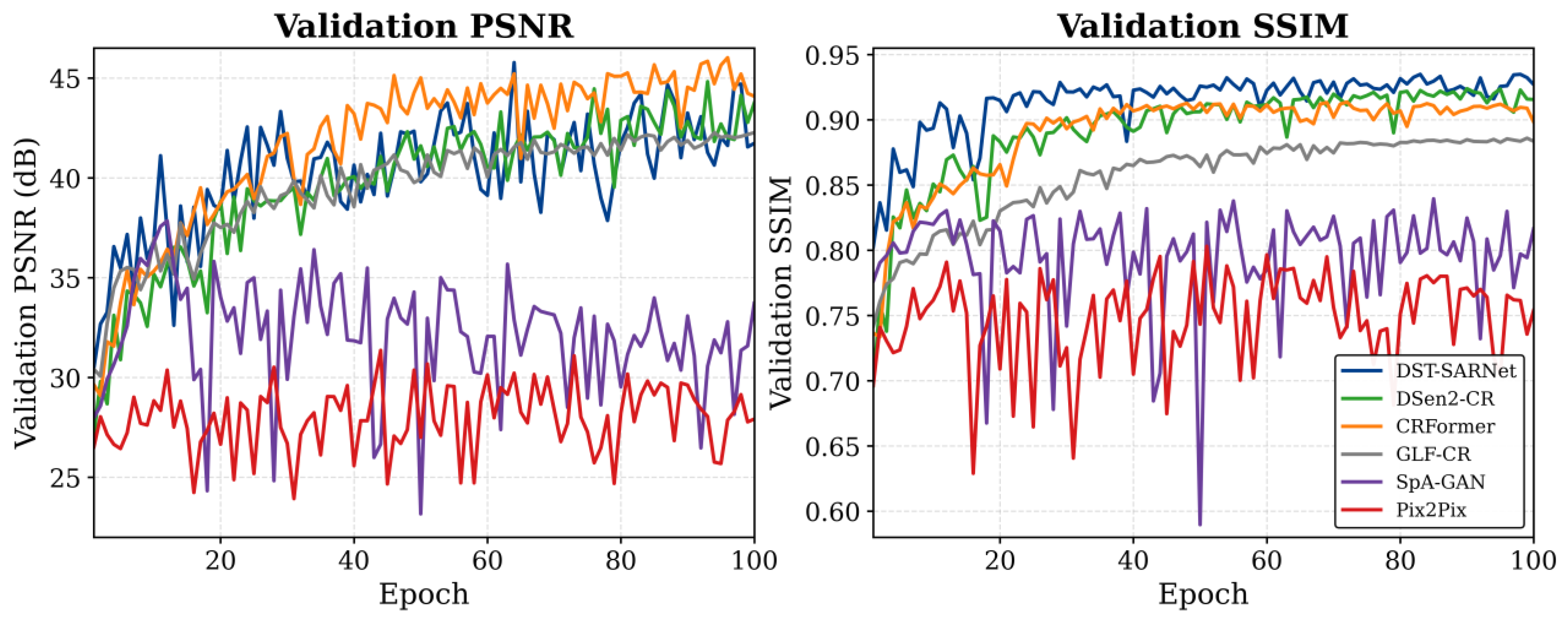
Figure 12 shows the validation PSNR and validation SSIM curves of different models during training. These curves reflect final validation performance, optimization convergence speed, training stability, and differences among structural designs during feature learning. For remote sensing cloud removal, the absence of surface information in thick-cloud regions significantly increases reconstruction uncertainty. Oscillation, convergence speed, and later-stage stability therefore provide indirect evidence of whether the model uses auxiliary structural information effectively.

Figure 12 shows that DST-SARNet obtains high validation SSIM early in training and maintains a relatively stable upward trend in later epochs. DSen2-CR and CRFormer also show stable training behavior, but their final reconstruction metrics are lower than those of DST-SARNet. The curves of SpA-GAN and Pix2Pix fluctuate more strongly, indicating that GAN-based generative models are more susceptible to adversarial optimization instability in cloud-contaminated remote sensing restoration. In contrast, the SSIM curve of DST-SARNet enters a stable interval faster, suggesting that structural similarity is recovered within fewer epochs. This behavior is consistent with the model design: the SAR structural skeleton constrains the spatial layout of cloud-hidden surfaces, and the optical backbone then learns color, semantics, and residual correction, transforming restoration from unconstrained image generation into optical reconstruction under structural conditions.

The different behaviors of the PSNR and SSIM curves can be explained by metric sensitivity and the nature of thick-cloud restoration. PSNR is derived from mean squared pixel error and is therefore highly sensitive to small radiometric deviations in cloudy regions, including slight changes in brightness, color residuals, and high-frequency texture intensity. During later epochs, the model may continue to adjust these pixel-level radiometric details under structural constraints, producing visible PSNR oscillations even when the recovered spatial organization is already stable. By contrast, SSIM measures local luminance, contrast, and structural consistency within image windows; once the main boundaries, texture directions, and local topology have been recovered, SSIM changes more slowly and remains comparatively stable. For GAN-based baselines, adversarial optimization further increases pixel-level variability, which explains the stronger PSNR fluctuation in SpA-GAN and Pix2Pix. Thus, the observed oscillation does not indicate unstable structural learning; rather, it shows that pixel-level radiometric fitting is more sensitive than structure-level similarity, while the SAR structural skeleton and optical-dominant reconstruction branch help stabilize the structural component of restoration.

In DST-SARNet, the adversarial component is used as a controlled perceptual refinement term rather than as the main reconstruction objective. The discriminator is introduced only after a reconstruction warm-up stage. The adversarial weight is kept small, and the least-squares GAN objective is combined with gradient clipping to reduce abrupt discriminator dominance. Under this strategy, the validation curves do not show persistent divergence or mode collapse. The remaining PSNR oscillation mainly reflects radiometric adjustment at the pixel level, whereas SSIM remains comparatively stable once the main spatial structures are recovered. The comparison between the non-adversarial variant and the full model further illustrates this trade-off: adversarial optimization slightly weakens strict pixel fidelity but improves perceptual consistency and texture naturalness.

Rapid SSIM convergence does not mean that final image quality can be judged by a single metric. SSIM mainly characterizes local structural similarity; therefore, early stabilization more directly reflects that the model has recovered spatial organization such as roads, water boundaries, farmland parcels, and mountainous textures. Color consistency, perceptual naturalness, and detail realism still require joint evaluation with PSNR, FID, LPIPS, and qualitative visualization. The positive implication is that the model can form a reliable structural framework at lower training cost, reduce dependence on long training or multi-step sampling for engineering deployment, and improve stability in model selection during training.

Compared with diffusion-based cloud removal methods, DST-SARNet uses single-pass inference and does not require multi-step sampling. Although perceptual constraints are introduced during training, the discriminator does not participate in inference; thus, deployment cost is determined by the generator backbone. DST-SARNet achieves high reconstruction quality with a low parameter count, indicating that its design is closer to an efficient direct reconstruction framework than to approaches relying on long sampling chains or large parameter capacity.

From an efficiency perspective, DST-SARNet does not pursue the highest FPS or the lowest FLOPs as the sole objective. Instead, it balances reconstruction quality, model scale, and inference speed. Some lightweight or GAN-based methods have higher inference speed, but their PSNR, SSIM, FID, and LPIPS results are clearly weaker than those of DST-SARNet. Some residual-network- or Transformer-based methods achieve stable reconstruction but usually require larger computation or more parameters. DST-SARNet reduces the cost of long-range dependency modeling through efficient global context modeling and avoids unnecessary multi-layer cross-modal fusion through selective SAR structural guidance, enabling strong thick-cloud restoration with a compact parameter scale.

Overall, the experimental results demonstrate that DST-SARNet achieves a favorable balance among reconstruction accuracy, visual quality, module contribution, computational efficiency, and training stability. On cloud-contaminated SMILE-CR test samples, DST-SARNet obtains better PSNR, SSIM, FID, and LPIPS than the comparison methods, showing improvements in both pixel-level reconstruction accuracy and the perceptual quality of restored cloud regions. Ablation experiments on challenging thick-cloud samples further show that SSG, TAAR, and LSGM contribute to cloud-hidden structural constraint, deep texture compensation, and output-stage high-frequency detail restoration, respectively. The training curves show that the model reaches stable structural similarity at an early stage, indicating that structure–appearance decoupling helps reduce uncertainty in thick-cloud restoration. Compared with baselines relying only on optical inputs or dense feature generation, DST-SARNet reduces the difficulty of thick-cloud restoration through controlled use of SAR structural priors and maintains competitive inference efficiency with a compact parameter scale.

4. Discussion

This section discusses the main phenomena revealed by the experiments. The analysis focuses on four aspects: performance under different cloud-contamination strengths, the role of selective SAR structural guidance, the relationship between perceptual quality and pixel fidelity, and the quality–efficiency trade-off. The Section 3 reports metrics and visual comparisons, whereas the Discussion explains the mechanisms behind these observations and clarifies the applicable boundaries of the method.

According to the SMILE-CR testing protocol, the test samples are divided into different degradation groups, including all test samples, cloud-contaminated samples, medium-to-high cloud-contamination samples, challenging thick-cloud samples, and input-near-clear samples. This grouping does not correspond to strict physical cloud-cover-rate intervals; instead, it is used to observe model performance under different degradation strengths from an evaluation perspective. Such analysis avoids misinterpreting the difference between cloudy input and reference imagery as cloud-cover rate, while still revealing model stability from weak to strong degradation conditions.

4.1. Performance Variation Under Increasing Restoration Difficulty

From all test samples, to cloud-contaminated samples, and then to challenging thick-cloud samples, the missing degree of cloud-hidden structures and optical reflectance gradually increases. If a model mainly relies on residual textures or local context in the cloudy optical image, its performance usually drops noticeably on difficult samples. Figure 13 presents the PSNR and SSIM gains of DST-SARNet over representative baselines across three evaluation subsets. Compared with absolute metric curves, this figure more directly reflects how the gap between methods changes as restoration difficulty increases.

The all-sample subset includes a portion of input-near-clear samples; therefore, some baselines are not far from DST-SARNet in this subset. For example, on all test samples, CRFormer has slightly higher PSNR than DST-SARNet, whereas DST-SARNet maintains an advantage in SSIM. When the evaluation shifts to cloud-contaminated samples and challenging thick-cloud samples, the advantages of DST-SARNet over CRFormer, DSen2-CR, and GLF-CR become more pronounced. This pattern indicates that the main benefit of the proposed model is concentrated in cloud-contaminated areas where optical information is more severely missing and structural-restoration uncertainty is higher, rather than in easy samples.

Table 7. Stability comparison among sample groups with different cloud-contamination strengths.

Method	All-Sample PSNR	Cloud-Affected PSNR	Thick-Cloud PSNR	Thick-Cloud SSIM	Thick-Cloud MAE	PSNR Drop
DST-SARNet (Ours)	44.49	36.58	33.73	0.8432	0.0172	10.77
CRFormer	44.57	33.77	30.21	0.7794	0.0313	14.36
DSen2-CR	43.20	33.53	29.87	0.8135	0.0272	13.33
GLF-CR	42.70	31.51	28.00	0.7209	0.0318	14.69
SpA-GAN	34.24	29.57	26.38	0.7035	0.0479	7.86
Pix2Pix	30.84	29.10	26.78	0.6804	0.0474	4.06
AttentionGAN	37.10	28.23	23.13	0.6306	0.0712	13.97

Note: PSNR drop denotes the difference between PSNR on all test samples and PSNR on challenging thick-cloud samples. This value should be interpreted together with the absolute PSNR of the challenging thick-cloud group; a smaller drop does not necessarily indicate higher restoration quality.

further reports stability statistics for different degradation groups. DST-SARNet achieves a PSNR of 33.73 dB, an SSIM of 0.8432, and an MAE of 0.0172 on challenging thick-cloud samples, outperforming the main comparison methods on all three metrics. PSNR degradation should be interpreted together with the absolute quality on the challenging thick-cloud group. The PSNR drop from all samples to challenging thick-cloud samples is smaller for Pix2Pix mainly because its starting point on all samples is already low; this does not necessarily indicate better thick-cloud restoration stability. In contrast, DST-SARNet maintains a high quality lower bound across all samples, cloud-contaminated samples, and challenging thick-cloud samples, indicating that early SAR skeletons and late detail modulation provide effective constraints when optical information is missing, and thereby reduce structural-guessing errors under thick-cloud conditions.

4.2. Structural Recovery Advantages on Challenging Thick-Cloud Samples

The key challenge in challenging thick-cloud samples is not only to remove visible clouds but also to recover credible structures when surface textures and spectral responses are extensively obscured. Traditional CNN-based methods tend to interpolate from local neighborhoods, generative methods may produce visually smooth but semantically unreliable textures, and standard Transformer-based methods may still smooth fine-grained edges and small-scale textures despite their long-range modeling ability. The advantage of DST-SARNet comes from structure–appearance decoupling: the SAR branch provides structural cues such as roads, water boundaries, farmland textures, and building outlines, while the optical backbone remains responsible for color and multispectral appearance recovery.

Figure 14 shows model differences on challenging thick-cloud samples from the perspective of performance gains and ranks the main baselines by their relative gaps. Compared with CRFormer, DST-SARNet improves PSNR by 3.52 dB and SSIM by 0.0638 on challenging thick-cloud samples. Compared with DSen2-CR, PSNR increases by 3.86 dB and SSIM by 0.0297; compared with GLF-CR, PSNR increases by 5.72 dB and SSIM by 0.1223. CRFormer has FLOPs close to those of DST-SARNet but lacks SAR structural skeletons and late spatial modulation, leading to insufficient boundary constraints in thick-cloud regions. Although DSen2-CR fuses SAR and optical inputs, its high computational cost does not translate into better thick-cloud restoration quality. These results indicate that multimodal input alone does not guarantee structural restoration advantages; the key factor is whether SAR information enters the network in an appropriate form.

This phenomenon can be further understood together with the qualitative thick-cloud samples in the Section 3. DST-SARNet produces outputs closer to the cloud-free reference in mountainous textures, riverbank boundaries, farmland parcels, and urban textures, consistent with the PSNR and SSIM gains in Figure 14. Compared with repeatedly injecting SAR as an ordinary input channel, selective structural guidance allows SAR to act at the most critical positions for structural constraint and high-frequency compensation while reducing the cumulative propagation risk of SAR speckle and cross-modal discrepancies in intermediate layers.

AFR-CR provides a representative frequency-domain perspective for SAR-assisted cloud removal. It emphasizes adaptive frequency-domain feature reconstruction, in which low-frequency structural components and high-frequency detail components are decoupled and reconstructed to enhance texture recovery. DST-SARNet addresses thick-cloud restoration from a different perspective. Instead of explicitly decomposing SAR–optical features in the frequency domain, it controls where and how SAR information enters the reconstruction process: SSG converts SAR into early structural skeletons, TAAR retrieves SAR structural memory under optical semantic queries, and LSGM applies Late SAR-Guided Spatial Modulation near the output stage. AFR-CR therefore focuses mainly on frequency-domain reconstruction, whereas DST-SARNet focuses on perturbation-controlled SAR structural guidance and output-stage high-frequency compensation. These two routes are complementary in motivation, while DST-SARNet further emphasizes reducing repeated intermediate SAR fusion and preserving the optical branch as the dominant source of spectral appearance.

4.3. Pixel Fidelity, Perceptual Quality, and Module Behavior

The ablation experiments show that different modules in DST-SARNet correspond to different optimization objectives; therefore, the results should not be interpreted as strict improvement in all metrics after each module is added. The optical-only efficient global context variant mainly reflects changes in global modeling and efficiency, but optical input alone cannot solve structural absence in thick-cloud regions. After the SAR structural skeleton is added, PSNR, SSIM, and LPIPS all improve noticeably, indicating that Stage-I structural priors reduce inference uncertainty in thick-cloud regions. Further introducing TAAR and late SAR spatial modulation continues to improve PSNR and SSIM on thick-cloud samples, showing that SAR structural memory retrieval and pre-output high-frequency modulation compensate texture attenuation in backbone features.

The non-adversarial variant achieves the highest PSNR and SSIM on challenging thick-cloud samples, indicating that reconstruction and structural losses are more favorable for optimizing pixel-wise similarity. Compared with this variant, the full model slightly reduces PSNR and SSIM on the hardest subset but substantially improves perceptual quality, as reflected by LPIPS and visual texture naturalness. This trade-off is important for remote sensing cloud removal. Applications requiring quantitative reflectance consistency may prefer the non-adversarial setting, whereas visual interpretation and scene understanding may benefit from the full model. In this paper, the full model is retained as the final configuration because it provides stronger perceptual realism while maintaining competitive pixel fidelity and stable overall performance on cloud-contaminated and challenging thick-cloud samples.

4.4. Quality–Cost Trade-Off and Convergence Behavior

Cloud removal models require not only high-quality reconstruction but also practical deployability. Large-area remote sensing imagery usually contains many image patches, and excessive parameter count or computational cost limits the use of models in regional-scale or long-term time-series tasks. Figure 15 shows the relationship between PSNR and FLOPs on cloud-contaminated samples. This figure does not repeat the computational-efficiency bar chart in the Section 3; instead, it presents model positions from the perspective of quality–cost trade-off.

Figure 15 shows that DST-SARNet lies in a favorable quality–cost trade-off region. Compared with CRFormer, DST-SARNet has similar FLOPs but higher PSNR. Compared with DSen2-CR, DST-SARNet has substantially lower computational cost while achieving higher reconstruction quality. Pix2Pix has the lowest FLOPs and highest FPS, but its PSNR, SSIM, and perceptual quality are insufficient for thick-cloud structural recovery. AttentionGAN and SpA-GAN have speed advantages, but their absolute quality on thick-cloud samples is relatively low, illustrating the difference between speed-oriented models and high-fidelity cloud removal models.

4.5. Potential Benefits for Downstream Remote Sensing Interpretation

Restored cloud-free images are also relevant to downstream remote sensing interpretation. Land-cover classification and segmentation require continuous spectral responses, recognizable spatial patterns, and clear object boundaries. By recovering field boundaries, roads, water edges, urban blocks, and vegetation textures, cloud removal may provide more complete inputs for these tasks. Change detection may also benefit because cloud contamination can create false changes between multi-temporal observations. Restoring cloud-contaminated regions can improve temporal comparability and reduce cloud-induced inconsistencies. Recent studies on adverse-condition change detection, interactive high-resolution change detection, and multi-scale decision fusion further suggest that degraded imaging conditions and spatial detail loss can affect interpretation reliability [10,42,43]. These benefits remain as potential rather than being quantitatively verified in this study because no task-specific classifier, segmenter, or change detector is trained. Future work should evaluate whether the improved structural fidelity and perceptual quality translate into measurable gains in land-cover mapping, segmentation, change detection, disaster monitoring, and ecological assessment.

4.6. Applicability Scope and Limitations of Selective SAR Guidance

Selective SAR guidance can be extended to other cross-modal remote sensing restoration tasks when one modality mainly provides structural cues and another modality provides appearance or spectral information. Potential applications include SAR-assisted optical missing-information reconstruction, cloud-shadow removal, cross-sensor gap filling, and optical–SAR fusion under persistent cloud cover. In these scenarios, the main principle is not to inject the auxiliary modality at every layer, but to transform it into structural priors, readable memory, or late detail modulation according to the degradation type and the reliability of cross-modal correspondence.

Selective SAR guidance has broad potential for cross-modal remote sensing restoration because many applications contain an auxiliary modality that preserves structural information when optical appearance is degraded. Its applicability is particularly promising for persistent-cloud monitoring, SAR-assisted optical gap filling, cloud-shadow restoration, and multisensor image fusion. In practical deployment, however, the strength of SAR guidance should depend on the reliability of cross-modal correspondence. Severe SAR–optical misregistration, large acquisition-time gaps, land-cover change, water-level variation, crop phenology, construction activity, weak scattering–appearance correlation, SAR shadow, layover, and strong speckle may reduce the usefulness of SAR-derived structures. These issues do not negate the value of SAR guidance; rather, they indicate that future extensions should incorporate confidence-aware gating, deformable alignment, temporal-consistency checking, and uncertainty estimation, so that SAR evidence can be adaptively emphasized when reliable and attenuated when it is not.

5. Conclusions

This paper proposes DST-SARNet for SAR-assisted cloud removal in optical remote sensing images. The method aims to recover cloud-free imagery with reliable spatial structures and visual consistency under thick-cloud occlusion. DST-SARNet transforms SAR from a repeatedly concatenated auxiliary channel into three controlled forms: structural skeletons, structural memory, and high-frequency modulation signals. SSG extracts cloud-hidden contours and texture directions at the input side. EGCB provides efficient global context modeling. TAAR retrieves SAR structural memory under optical semantic control. LSGM compensates for high-frequency details before final reconstruction.

Experiments on SMILE-CR show that DST-SARNet outperforms the main comparison methods in PSNR, SSIM, FID, and LPIPS on cloud-contaminated samples and maintains stable advantages on challenging thick-cloud samples. Additional experiments on SEN12MS-CR further validate its adaptability under Sentinel-2 multispectral imagery and Sentinel-1 SAR conditions. Ablation experiments demonstrate that the SAR structural skeleton, texture-aware retrieval, and late spatial modulation contribute to structural constraints, texture compensation, and high-frequency detail restoration, respectively. Quality–efficiency analysis and training curves further show that DST-SARNet does not rely on a larger parameter scale or long sampling chain; instead, it achieves strong reconstruction quality with a compact model scale, lower training cost, and practical computational expense. Future work will focus on robustness under SAR speckle noise and cross-modal registration errors, cross-region, cross-season, and cross-sensor generalization, and downstream evaluations such as land-cover classification, change detection, and disaster monitoring to assess the practical value of cloud removal results.