Long-Term Monitoring of Saline–Alkaline Land Converted to Paddy Fields Using a Time-Series Change Detection Algorithm

Highlights

What are the main findings?

• An MK-based Landsat time-series framework was developed to detect saline–alkaline land conversion to paddy fields.
• June SI5 was the most effective spectral indicator, enabling accurate mapping of conversion extent and timing.

What are the implications of the main findings?

• The proposed framework supports long-term remote sensing monitoring of saline–alkaline land reclamation.
• The results provide useful evidence for sustainable paddy-field expansion and land-resource management in saline–alkaline regions.

Abstract

Saline–alkaline land serves as a potential arable land reserve for augmenting agricultural productivity and safeguarding food security. However, long-term monitoring of saline–alkaline land conversion remains challenging because of vegetation recovery, surface changes, hydrological modification, and agricultural phenology. Compared with CCDC and LandTrendr, the proposed MK-based framework detects conversion occurrence and timing while reducing dependence on dense observations, parameter tuning, and annual classification. This study examines the spatiotemporal dynamics of saline–alkaline land converted into paddies in Da’an City, utilizing Landsat time-series data (2007–2021) from the Google Earth Engine (GEE) platform. The analysis employed Mann–Kendall (MK) trend and mutation tests to monitor conversion processes and analyze spatiotemporal dynamics. Point-biserial correlation analysis was applied to evaluate the sensitivity of various remote sensing indices in detecting land conversion. The top fifteen indices, including the Land Surface Water Index (LSWI), Salinity Index 4 (SI4), and Salinity Index 5 (SI5), demonstrated strong correlations (|r| = 0.788–0.885) and significant pre- and post-conversion spectral differences (p < 0.01). Validation via confusion matrix confirmed that the June SI5 index attained the highest detection accuracy (overall accuracy: 94.15%; Kappa coefficient: 0.86), supporting the MK trend test’s efficacy in monitoring conversion processes. The MK mutation test achieved 80.36% temporal accuracy in determining conversion timing. The spatiotemporal analyses identified heterogeneity in saline–alkaline land conversion patterns. Spatially, large contiguous paddy fields dominated the eastern region, whereas fragmented conversion characterized the west, with minimal activity in the central zone. Temporally, the conversion area expanded rapidly before 2015 and then gradually declined, reaching a cumulative converted area of 276.29 km² by 2021. This study elucidates spatiotemporal conversion dynamics to guide sustainable land use.

1. Introduction

As a critical reserve of arable land, saline–alkaline land offers significant potential for expanding arable land. Through scientific reclamation and rational development, saline–alkaline land can help address the global food crisis and contribute to food security [1]. In addition, reclaiming saline–alkaline land has the potential to increase food production and promote more efficient land use, while the hydrological environmental impacts associated with conversion to paddy fields should also be considered [2,3]. For instance, converting 7.43 × 10⁵ ha of saline–alkaline land in western Jilin Province into paddy fields resulted in the potential to increase rice yields from 1.11 × 10⁶ t to 5.94 × 10⁶ t [4]. In recent decades, significant advancements in reclamation technologies have been achieved, including gypsum application, deep tillage, soil remediation, and the development of salt-tolerant crop varieties that have collectively improved soil structure and fertility, facilitating the cultivation of rice and other food crops [2]. Supported by technological innovations and policy incentives, converting saline–alkaline land into paddy fields has emerged as a predominant land-use strategy in western Jilin Province, China. Long-term monitoring of this conversion process remains highly challenging because it involves substantial and persistent surface changes, while traditional field surveys are time-consuming and difficult to sustain [5]. In contrast, remote sensing technology provides a spatially comprehensive, temporally flexible, and cost-efficient monitoring framework, rendering it a powerful tool for monitoring land use changes [6].

Advancements in the spatiotemporal resolution of remote sensing imagery, combined with systematic large-scale observations and extended temporal data archives, have significantly enhanced the capabilities of remote sensing for detecting land use changes [7]. Remote sensing technologies are applied in a plethora of areas, including deforestation monitoring, drought monitoring, urban expansion analysis, agricultural reclamation and intensification, and disaster assessment [8,9]. Supervised change detection methodologies are based on change detection principles and temporal image availability and predominantly employ bi-temporal or multitemporal image sequences [10]. Three principal methodological frameworks exist for bi-temporal change detection: (1) image arithmetic-based, (2) image transformation-based, and (3) post-classification methods [11]. The principal advantage of post-classification methods lies in generating explicit “from-to” change information. This methodology exhibits robustness against atmospheric disturbances, seasonal variations, and sensor heterogeneity, enabling cross-seasonal and cross-sensor comparisons [12], and currently represents one of the most widely used techniques in change detection research. However, its efficacy is contingent upon classification accuracy, as errors propagate into the final change maps [13]. Bi-temporal change detection frameworks are constrained to binary temporal comparisons and thus cannot adequately capture longitudinal landscape dynamics [14]. These limitations highlight the need for time-series methods that can capture continuous surface changes and identify the timing of land conversion.

The conversion of saline–alkaline land to paddy fields involves both gradual vegetation recovery and abrupt surface changes driven by reclamation activities and water management. These characteristics make it necessary to use methods that can capture gradual trends and detect change points within long-term remote-sensing time series. With the growing accumulation of remote sensing datasets, time-series change detection algorithms capable of characterizing continuum surface processes have emerged as the predominant methodological paradigm for land use change detection [15]. Three principal algorithmic frameworks, Breaks for Additive Season and Trend (BFAST), Landsat-based Detection of Trends in Disturbance and Recovery (LandTrendr), and Continuous Change Detection and Classification (CCDC), have achieved widespread implementation in contemporary geospatial analysis [16]. The BFAST algorithm detects changes by decomposing time-series data into trend, seasonal, and remainder components, followed by calculating the sum of squared residuals [17]. However, while BFAST demonstrates computational efficiency in fine-scale disturbance detection, its operational robustness is critically dependent on temporal signal-to-noise characteristics [18]. The LandTrendr framework identifies long-term gradual changes and short-term abrupt disturbances through piecewise linear temporal segmentation [19,20]. However, applying it requires a series of control parameter tuning and filtering steps to minimize overfitting during time segmentation. The CCDC framework employs harmonic regression modeling to establish phenological baselines, flagging persistent deviations as landscape change events [21]. Although CCDC can detect inter- and intra-annual trends, it requires sufficient clear observations and may be less effective in highly variable agricultural landscapes [22]. These approaches usually require dense and relatively stable temporal observations or parameter tuning, and their performance may be affected by agricultural phenology, spectral mixture, and intra-annual variability in saline–alkaline reclamation landscapes. The Mann–Kendall (MK) nonparametric statistical framework demonstrates strong resilience to data anomalies and distribution-free operation, requiring no prior assumptions regarding the normality of these data [23]. The MK test can identify monotonic trends in time-series data, while the MK mutation test can detect potential change points by comparing forward and backward statistical sequences. Therefore, combining the MK trend test and MK mutation test can support the identification of both conversion occurrence and conversion timing in saline–alkaline land conversion monitoring. Hu et al. [24] employed MK trend and mutation tests to assess vegetation recovery and identify stabilization timing in mine reclamation areas. The phased transition characteristics of saline–alkaline land conversion—initial rapid modification followed by progressive stabilization—create ideal conditions for MK-based change detection frameworks.

Since 2010, western Jilin Province has spearheaded large-scale agricultural reclamation initiatives, systematically converting 1.32 million hectares of saline–alkaline soils into productive paddy fields [25]. This transformative program has promoted regional agricultural development, optimized land use, and contributed to ecological restoration. Despite the large scale of this conversion, a time-series monitoring framework is still needed to characterize its spatial extent, temporal trajectory, and conversion timing at regional scales. In this study, the MK statistical framework on Google Earth Engine (GEE)’s cloud-based geospatial processing platform establishes an integrated monitoring system for spatiotemporal pattern analysis of saline–alkaline land conversion dynamics. The methodological novelty of this study lies in integrating spectral index–month sensitivity analysis with MK trend and mutation tests to identify conversion occurrence and timing without annual land-cover pre-classification. This research aims to evaluate the sensitivity of 25 spectral indices, validate MK-based change detection, and characterize the spatiotemporal dynamics of saline–alkaline land conversion during 2007–2021. The implementation of robust monitoring frameworks for these complex land transformation processes enables evidence-based policymaking, optimizing the trade-offs between agricultural productivity and socio-ecological sustainability in global saline–alkaline regions.

2. Materials and Methods

2.1. Overview of the Study Area

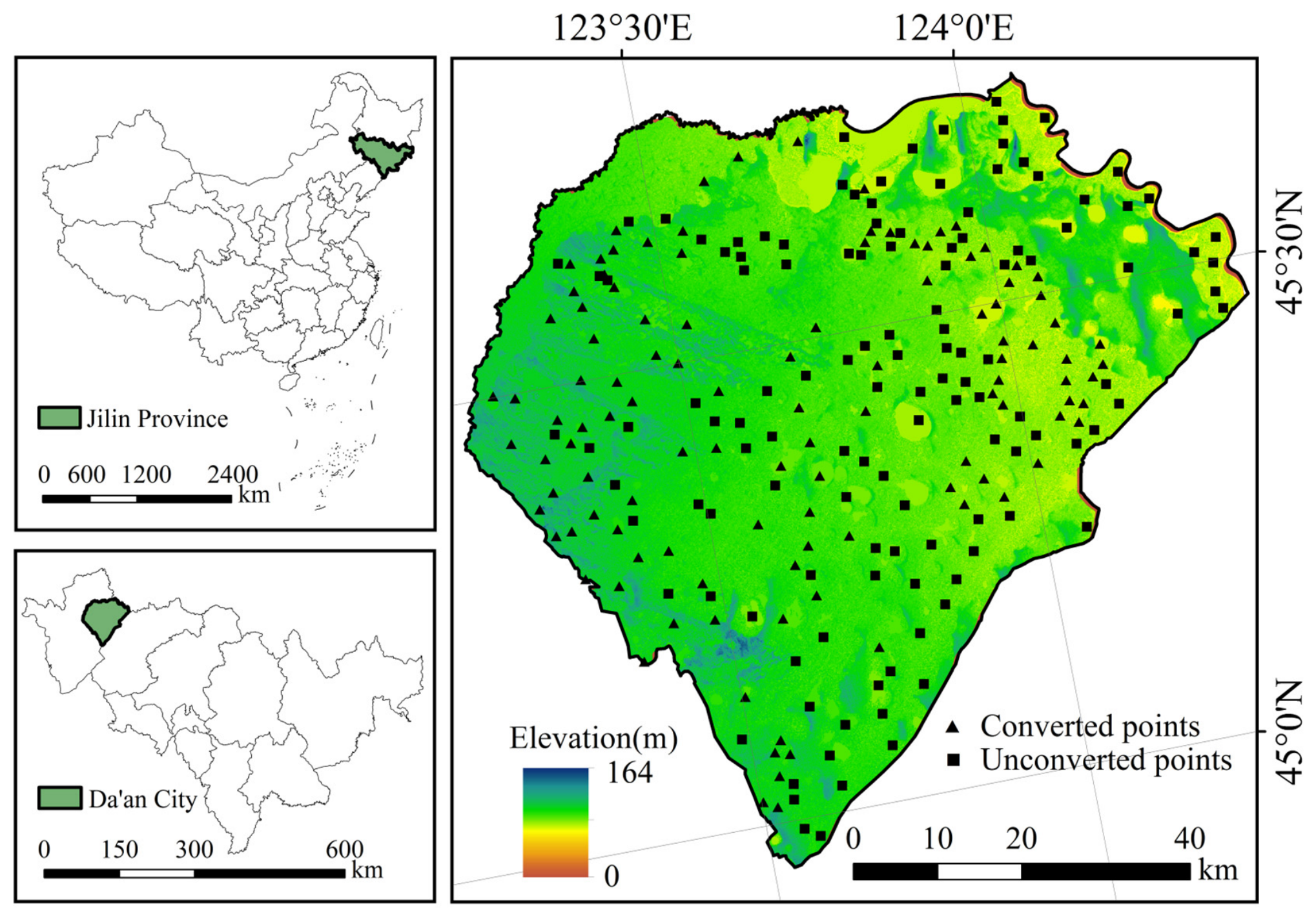
Da’an City is situated in the northwest of Jilin Province, China, spanning 123°08’–124°21’E and 44°57’–45°45’N (Figure 1). The city stretches 95 km east–west and 90 km north–south, encompassing a total area of approximately 4878.59 km². The region experiences a temperate continental monsoon climate with distinct seasonal variations. The average annual precipitation ranges from 400 to 500 mm, of which 82.8% occurs during summer. The annual evaporation ranges from 1250 to 1650 mm, classifying it as a semi-arid region [26]. Chernozems and meadow soils dominate the area. Characterized by flat terrain with gentle undulations, Da’an City lies within the low-lying Songnen Plain, where numerous lakes and marshes are distributed. The saline–sodic soils in this plain primarily contain Na₂CO₃ and NaHCO₃, ranking it among the world’s three largest saline–sodic soil regions. Due to its unique climatic and geographical conditions, Da’an City exhibits a pronounced accumulation of soil salinity, rendering it the most severely salinized area within the Songnen Plain [27]. In 2008, the Western Land Development and Consolidation Project promoted saline–alkaline land reclamation through rice cultivation, supported by major water conservancy infrastructure such as the Da’an Irrigation District and the Hadashan Hydrojunction [28].

2.2. Data Sources and Processing

2.2.1. Field Surveys

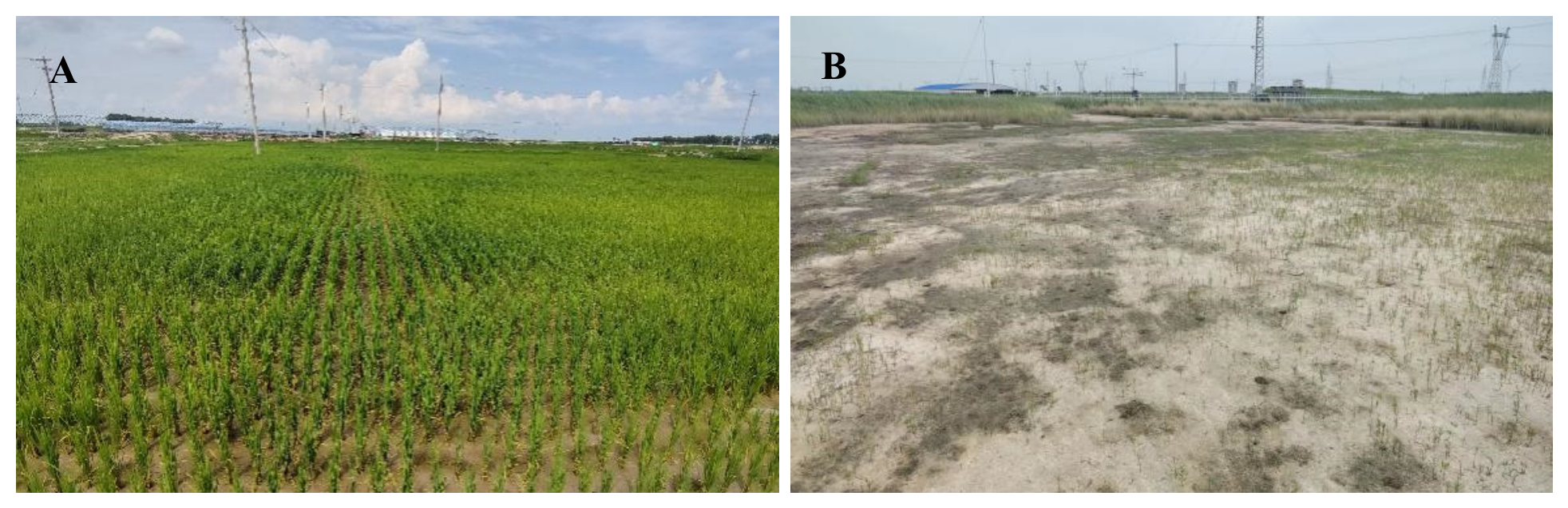
During July–August 2023, a field survey was conducted in the study area to develop a remote sensing monitoring model for saline–alkaline-to-paddy field conversion and validate its accuracy. Conversion status and conversion year were determined by combining field observations with visual interpretation of historical high-resolution DigitalGlobe imagery available in Google Earth and Landsat time-series images. Specifically, converted sites were identified as areas that showed a transition from saline–alkaline land in historical imagery to paddy fields in subsequent imagery and field observations. Unconverted sites were defined as areas that showed no such transition during the study period and served as negative/reference samples for assessing commission errors in conversion detection. This survey documented conversion status (converted/unconverted), conversion year, and land use history. Sampling points maintained >2 km separation, with plot dimensions exceeding 100 m × 100 m, to ensure spatial independence and reduce autocorrelation. The >2 km distance threshold was used to minimize spatial clustering among validation samples. The plot size threshold was set to exceed a 3 × 3 Landsat pixel window at 30 m resolution, which improved sample representativeness and reduced mixed-pixel effects [29]. A total of 227 georeferenced sampling points were selected, including 112 converted (saline–alkaline-to-paddy field conversion) and 115 unconverted sites. The unconverted sites included 70 persistent saline–alkaline areas, 20 stable paddy fields, and 25 permanent water bodies (Figure 1). Geographic coordinates were acquired at plot centroids using a Newmap P30 Real-Time Kinematic (RTK) system with ±2 cm positional accuracy. Landscape photographs documenting site characteristics were archived systematically (Figure 2). Sampling locations were strategically positioned in agricultural zones ≥ 300 m from transportation corridors and settlements to minimize mixed-pixel interference, with explicit exclusion of vertical features (e.g., trees, infrastructure) within 50 m radii.

2.2.2. Landsat 5 Tm and Landsat 8 Oli Time-Series Data

Compared with Sentinel-2 and the MODIS dataset, Landsat series data more effectively encompass the temporal coverage and spatial resolution requirements of this study. Due to striping artifacts in Landsat 7 data post-2003, Landsat 5 TM and Landsat 8 OLI datasets were selected as the primary data sources. The parameters of the bands used in this study are shown in

Table 1. Band parameters of Landsat 5 and Landsat 8.

Color	Landsat 5		Landsat 8
	Band Specification	Wavelength (nm)	Band Specification	Wavelength (nm)
Blue	Band 1	450–520	Band 2	452–512
Green	Band 2	520–600	Band 3	533–590
Red	Band 3	630–690	Band 4	636–673
NIR	Band 4	770–900	Band 5	851–879
SWIR1	Band 5	1550–1750	Band 6	1566–1651
SWIR2	Band 7	2080–2350	Band 7	2107–2294

.

Data in this research were obtained from the GEE platform, specifically the “LANDSAT/LT05/C02/T1_L2” and “LANDSAT/LC08/C02/T1_L2” data products, which have been pre-processed for radiometric calibration, atmospheric correction, and geometric correction. A cloud mask was generated using the QA_PIXEL band within the GEE-hosted Landsat products, facilitating efficient cloud removal from the selected imagery.

2.2.3. Land Cover Data

To mitigate interference from nontarget land conversions, a 30-m resolution land use dataset developed by Yang & Huang [30] through GEE-based processing of 335,709 Landsat scenes was adopted. This dataset, classified using a random forest classifier after constructing multiple temporal metrics, yielded an OA of 79.31%, sufficiently meeting the required accuracy threshold. The 2007 saline–alkaline barren land layer was employed as a spatial mask to establish baseline conditions, ensuring exclusive focus on saline–alkaline-to-paddy transitions in the temporal analyses. This approach effectively removed interference from non-saline–alkaline regions, ensuring exclusive focus on saline–alkaline-to-paddy transitions in the temporal analyses.

2.2.4. Global 30 M Annual Wetland Maps

During the rice transplanting period (May–June), paddy fields and wetlands exhibit spectral similarity that may compromise classification accuracy, potentially compromising the accuracy of rice mapping [31]. This study employed the GWL_FCS30D dataset—an annual 30-m resolution global wetland product for the period 2000–2022, generated by Zhang et al. [32] using time-series Landsat imagery on the GEE platform—to address this spectral ambiguity. This dataset integrated global wetland training sample data and was generated using a locally adaptive classification method incorporating spatiotemporal consistency validation. It has an OA of 86.95 ± 0.44% and a KC of 0.822, satisfying the requirements of this study.

2.3. Data Analysis

This study used established methods, including the MK trend test, MK mutation test, and Otsu algorithm. The methodological contribution of this study lies in integrating these methods into a phenology-guided Landsat time-series framework for monitoring saline–alkaline land conversion. This framework combines spectral index–month sensitivity analysis, MK-based conversion occurrence detection, MK-based conversion-year identification, and wetland–water body masking. It therefore enables the detection of both conversion extent and timing while reducing dependence on annual land-cover pre-classification.

2.3.1. Selection of Spectral Indices

The land transformation process from saline–alkaline soils to productive paddies constitutes a tripartite biogeochemical transition, encompassing (a) EC dynamics, (b) vegetation community succession, and (c) hydroperiod modifications [33]. Accordingly, diagnostic spectral indices specifically sensitive to (i) saline signature, (ii) photosynthetic activity, and (iii) surface hydrology to quantify conversion efficacy were implemented. This triaxial monitoring framework simultaneously resolves (1) electrolytic gradient evolution, (2) vegetative canopy development, and (3) aquatic regime transitions, enabling comprehensive process characterization [34]. As the principal edaphic constraint, soil salinity dynamics constitute the pivotal conversion metric, quantifiable through electromagnetic signature analysis via dedicated salinity indices [35]. Vegetative spectral proxies diagnose rice phenological development through chlorophyll-sensitive band ratios [36]. Flooded paddies exhibit distinct electromagnetic signatures characterized by depressed reflectance in VNIR spectral regions (400–900 nm), providing diagnostic hydrological markers [37]. Hydrological indices leverage this spectral contrast to delineate spatiotemporal inundation patterns during critical rice cultivation stages [38]. In this study, a total of 25 spectral indices were selected, including 18 salinity discriminators, 4 vegetative phenology trackers, and 3 hydrological regime indicators (

Table 2. Calculation Formulae of Spectral Indices in this study.

Category	Spectral Indices	Abbreviation	Formula	References
Salinity-related spectral indices	Salinity index	SI	$\sqrt{B\times R}$	[41]
	Salinity index 1	SI1	$\sqrt{G\times R}$	[41]
	Salinity index 2	SI2	$\sqrt{G^2+R^2+{NIR}^2}$	[42]
	Salinity index 3	SI3	$\sqrt{ G^2+R^2}$	[42]
	Salinity index 4	SI4	$SWIR1/NIR$	[42]
	Salinity index 5	SI5	$\left(R-SWIR1\right)/\left(R+SWIR1\right)$	[43]
	Salinity index I	S1	$B/R$	[44]
	Salinity index II	S2	$\left(B-R\right)/\left(B+R\right)$	[44]
	Salinity index III	S3	$\left(G\times R\right)/B$	[44]
	Salinity index V	S5	$\left(B\times R\right)/G$	[44]
	Salinity index VI	S6	$\left(R\times NIR\right)/G$	[44]
	Intensity index 1	Int1	$\left(G+R\right)/2$	[42]
	Intensity index 2	Int2	$\left(G+R+NIR\right)/2$	[42]
	Vegetation soil salinity index	VSSI	$2\times G-5\times \left(R+NIR\right)$	[45]
	Canopy response salinity index	CRSI	$\sqrt{{\displaystyle \frac{NIR\times R-G\times B}{NIR\times R+G\times B}}}$	[46]
	Brightness index	BI	$\sqrt{ R^2+{NIR}^2}$	[41]
	three-band (3D) index5	TBI5	$\left(SWIR1+SWIR2\right)/B$	[47]
	three-band (3D) index7	TBI7	${\displaystyle \frac{\left(SWIR1-SWIR2\right)}{\left(SWIR2-B\right)}}$	[47]
Vegetation-related spectral indices	Normalized Difference vegetation index	NDVI	$\left(NIR-R\right)/\left(NIR+R\right)$	[48]
	Enhanced vegetation index	EVI	${\displaystyle \frac{2.5\times \left(NIR-R\right)}{\left(NIR+6\times R-7.5\times B+1\right)}}$	[49]
	Ratio vegetation index	RVI	$NIR/R$	[50]
	Soil-adjusted vegetation index	SAVI	${\displaystyle \frac{1.5\times \left(NIR-R\right)}{\left(NIR+R+0.5\right)}}$	[51]
Water-related spectral indices	Land Surface Water Index	LSWI	$\left(NIR-SWIR1\right)/\left(NIR+SWIR1\right)$	[52]
	Normalized Difference Water Index	NDWI	$\left(G-NIR\right)/\left(G+NIR\right)$	[53]
	Modified Normalized Difference Water Index	MNDWI	$\left(G-SWIR1\right)/\left(G+SWIR1\right)$	[54]

Note: B, G, R, NIR, SWIR1, and SWIR2 refer to the reflectance in visible blue, green, red, near-infrared, and shortwave infrared 1 and 2, respectively.

). Rice phenology dictates sequential agricultural phases (May–October): flooding → transplanting → irrigation → drainage → harvesting, generating temporally distinct spectral trajectories. Conversely, unaltered saline–alkaline areas exhibit minimal anthropogenic modification, with surface dynamics dominated by precipitation-driven geochemical processes [25]. This phenological window (May–October) maximizes surface heterogeneity between managed paddies and natural saline substrates, optimizing the sensitivity of change detection [39]. Multitemporal compositing was implemented via GEE’s seriesByRegion algorithm with the ‘ee.Reducer.mean()’ reducer, generating cloud-masked monthly synthetic products to mitigate radiometric anomalies. The surface characteristics of vegetation cover, water bodies, and soil backgrounds exhibit substantial seasonal variability during the rice-growing season, resulting in corresponding spectral changes [36]. In the monitoring of saline–alkaline land conversion into paddy fields, annual average spectral indices fail to acquire critical phenological signatures, limiting the detection of prominent temporal characteristics of the conversion process [40]. This study developed intra-annual homologous time series through phenological phase alignment, normalizing inter-annual comparisons while preserving seasonal signals. The temporal change patterns in paddy fields can be effectively acquired through this method, such as increased vegetation cover, water body dynamics, and other significant features, thus enhancing the sensitivity and accuracy of change detection.

2.3.2. Point-Biserial Correlation Analysis

In remote sensing, sensitivity is commonly quantified using statistical measures such as correlation coefficients, significance tests, and feature-importance metrics [55]. The point-biserial correlation coefficient is an appropriate statistic for assessing the association between a continuous variable (e.g., spectral index) and a binary variable (e.g., conversion vs. non-conversion) [56]. This approach has been widely applied in remote-sensing studies to quantify the sensitivity of vegetation- and water-related indices to land-surface processes [57]. To evaluate spectro-temporal sensitivity patterns, point-biserial correlation analysis was used to identify spectral indices and temporal windows exhibiting strong conversion signatures. Point-biserial correlation analysis quantifies linear associations between continuous variables (spectral indices) and dichotomous predictors (conversion status), with effect size measured through Pearson-derived coefficients [58]. This method requires minimal distributional assumptions and enables multiscale sensitivity assessments while maintaining computational efficiency [56]. Coefficient polarity (+/−) denotes the directionality of the relationship, while magnitude (0 ≤ r_pb ≤ 1) quantifies strength. In this study, spectral indices were treated as continuous variables, contrasted against binary conversion status (converted/unconverted) through dummy variable encoding. To ensure independence between method development and accuracy assessment, the 112 converted sampling points were randomly divided into a calibration subset (n = 56) and a validation subset (n = 56). A 50:50 split was adopted as a balanced holdout strategy because it kept the calibration and validation subsets comparable in size while maintaining independence between method development and accuracy assessment [59]. The calibration subset was used only for spectral-index screening, correlation analysis, and method development based on the pre- and post-conversion time-series information from converted sites, without including the 115 unconverted sites. It was not used in the accuracy assessment. The validation dataset consisted of the remaining 56 converted points and all 115 unconverted points, which were used only to assess detection accuracy.

2.3.3. Mann–Kendall Trend Test

The MK nonparametric framework detects monotonic temporal trends and critical transition points through rank-based significance testing [60]. This distribution-free approach demonstrates robustness against non-normal data distributions, extreme values, and sparse temporal observations. MK-based change detection has been extensively used in land system science for tracking LULC transitions, vegetation phenology shifts, and hydro-ecological dynamics [61]. The calculation formulae for the MK test are as follows:

$$S={\displaystyle \sum _{i=1}^{n-1}} {\displaystyle \sum _{j=i+1}^n} sgn(x_j-x_i)$$

(1)

$$sgn\left(x_j-x_i\right)=\left\{\begin{array}{ll}+1,& x_j-x_i>0\\ 0,& x_j-x_i=0\\ -1,& x_j-x_i<0\end{array}\right.$$

(2)

where x_j and x_i represent the pixel spectral index values in year j and year i, respectively, and n is the length of the time-series. If the pixel spectral index value in year j is greater than that in year i, the value of S is increased by 1. Conversely, the value of S decreases by 1 if year j is less than in year i. If the two values are equal, the value of S remains unchanged.

Var(S) represents the variance of the S value.

$$\mathrm{V}\mathrm{a}\mathrm{r}\left(S\right)={\displaystyle \frac{n\left(n-1\right)\left(2n+5\right)}{18}}$$

(3)

The test statistic Z is used to measure the trend. A positive Z value indicates an increasing trend, a negative Z value indicates a decreasing trend, and Z = 0 indicates no trend.

$$Z=\left\{\begin{array}{l}{\displaystyle \frac{S-1}{\sqrt{\mathrm{V}\mathrm{a}\mathrm{r}\left(s\right)}}},S>0\\ 0,\hspace{0.25em}S=0\\ {\displaystyle \frac{S+1}{\sqrt{\mathrm{V}\mathrm{a}\mathrm{r}\left(s\right)}}},S<0\end{array}\right.$$

(4)

$$p=2\left[1-\varphi \left(\left|Z\right|\right)\right]$$

(5)

Φ(Z) represents the cumulative distribution function of the standard normal variable. Statistical significance was evaluated through Z-score normalization and subsequent Φ(Z) computation from standard normal cumulative distribution. Significant conversions (p < 0.05) were identified when Φ(Z) exceeded critical thresholds, providing 95% confidence in trend rejection [62]. In this study, when the spectral values of the time series of a pixel show significant changes (p < 0.05), it indicates that the pixel has undergone a significant conversion, and the saline–alkaline land within the pixel is classified as having been converted into paddy fields.

2.3.4. Mann–Kendall Mutation Test

The MK mutation test is a nonparametric statistical test used to detect the onset of a mutation in a time series without requiring any assumptions regarding the distribution of the variables [60]. The specific calculation procedure is as follows:

$$S_k={\displaystyle \sum _{i=1}^k} r_i\left(k=2, \dots , n\right)$$

(6)

For a time-series r_i with n samples, the cumulative count S_k is calculated.

$$r_i=\left\{\begin{array}{c}1,x_i>x_j\\ 0,x_i\le x_j\end{array}\right. j=1,2,\dots ,n$$

(7)

when X_i > X_j, r_i is assigned a value of 1; otherwise, it is assigned 0. The cumulative count S_k represents the sum of instances where the pixel spectral index value of year i is greater than that of year j. Assuming the time series follows the same distribution, the test statistic is defined as follows:

$$U{F}_k={\displaystyle \frac{S_k-\mathrm{E}\left(S_k\right)}{\sqrt{\mathrm{V}\mathrm{a}\mathrm{r}\left(S_k\right)}}},(k=1,2,\dots ,n)$$

(8)

Here, UF₁ = 0. E (S_k) and Var (S_k) represent the mean and variance of the cumulative count S_k, which are calculated using the following formulae:

$$\mathrm{E}\left(S_k\right)={\displaystyle \frac{n\left(n-1\right)}{4}}$$

(9)

$$\mathrm{V}\mathrm{a}\mathrm{r}\left(S_k\right)={\displaystyle \frac{n\left(n-1\right)\left(2n+5\right)}{72}}$$

(10)

UF_k is a sequence of statistics calculated from the time series X₁, X₂, …, X_n. Then, the above process is repeated based on the reverse time series X_n, X_n−1, …, X₁ to obtain the sequence of UB_k statistics. The UF_k and UB_k curves were plotted by setting UB_k = −UF_k and UB₁ = 0. If the intersection of UF_k and UB_k falls within the 95% confidence interval, the corresponding year at the intersection point is determined as the starting time for the conversion of saline–alkaline land into paddy fields. When multiple intersections occur for the same pixel, the first valid intersection after the onset of a time-series trend consistent with the expected spectral change from saline–alkaline land to paddy fields is selected as the conversion year.

2.3.5. Otsu Algorithm to Extract Water

The Otsu method is an algorithm for automatically selecting a threshold from a grayscale histogram proposed by Otsu [63]. It is considered one of the most efficient methods for threshold determination [64]. The principle of this method relies on selecting an optimal threshold that maximizes the inter-class variance, thus effectively separating the background from the target object. In hydrographic feature extraction, Otsu’s method has demonstrated 93–97% segmentation accuracy across diverse aquatic environments [65]. Regional validation in Jilin’s water-related ecosystems achieved 95.2% classification accuracy using Otsu-optimized thresholds [66]. Landsat’s 16-day revisit cycle imposes temporal sampling constraints, particularly in dynamic phenological environments. Cloud contamination and seasonal precipitation frequently reduce usable acquisitions to <2 scenes/month, creating temporal data voids that challenge continuous monitoring [67]. These limitations necessitate multiyear data integration to reconstruct complete hydrological signatures. Fourteen-year hydrological archives (2007–2021) were compiled to compensate for annual data gaps through temporal compositing. The specific formulae are as follows:

$${\sigma }^2=W_0({\mu }_0-\mu {)}^2+W_1({\mu }_1-\mu {)}^2$$

(11)

$$W_0\times {\mu }_0+W_1\times {\mu }_1=\mu$$

(12)

$$W_0+W_1=1$$

(13)

where σ² represents the inter-class variance of water and land pixels; μ₀, μ₁, and μ represent the mean values of water pixels, land pixels, and all pixels in the remote sensing image, respectively; and W₀ and W₁ denote the proportions of water and land pixels in the image, respectively.

$$\underset{-1<t<1}{T=\mathrm{Arg\; max}}\left[{\sigma }^2\right]$$

(14)

For water extraction using MNDWI, whose theoretical values range from −1 to 1, the optimized threshold T ∈ [−1, 1] dichotomizes pixels into water (DN = 1 if X ≥ T) vs. non-water (DN = 0 if X < T), where X represents MNDWI values. Spectral confusion occurs during the May–June transplanting phases, when flooded paddies exhibit NIR-SWIR signatures analogous to permanent water bodies, introducing classification uncertainties [68]. A quantitative assessment of these phenology-induced errors is presented in Section 4.2.

2.4. Accuracy Assessments

2.4.1. Spatial Accuracy Assessment

Multisource validation frameworks integrating geotagged field photography, GNSS positioning, and multitemporal Google Earth imagery have been established as robust verification protocols in land cover mapping [69]. A hybrid validation protocol combining decadal high-resolution archives (Google Earth Pro 7.3) with field-measured data was implemented to obtain validation data for the MK test via visual interpretation. Spatial correspondence analysis constitutes the cornerstone of conversion detection validation, quantifying geolocational agreement between predicted and observed transitions. In this study, accuracy assessment was performed by constructing a confusion matrix and including the producer’s accuracy (PA), user’s accuracy (UA), overall accuracy (OA), and the Kappa coefficient (KC). The equations for these accuracy metrics are as follows:

$$\mathrm{P}\mathrm{A}={\displaystyle \frac{\mathrm{T}\mathrm{P}}{\mathrm{T}\mathrm{P}+\mathrm{F}\mathrm{N}}}$$

(15)

$$\mathrm{U}\mathrm{A}={\displaystyle \frac{\mathrm{T}\mathrm{P}}{T\mathrm{P}+\mathrm{F}\mathrm{P}}}$$

(16)

$$\mathrm{O}\mathrm{A}={\displaystyle \frac{\mathrm{T}\mathrm{P}+\mathrm{T}\mathrm{N}}{N}}$$

(17)

$$\mathrm{K}\mathrm{C}={\displaystyle \frac{N{\displaystyle \sum _{k=1}^q}{N}_{kk}-{\displaystyle \sum _{k=1}^q}{N}_{k+}{N}_{+k}}{N^2-{\displaystyle \sum _{k=1}^q}{N}_{k+}{N}_{+k}}}$$

(18)

where TP and TN represent the number of samples correctly identified as converted and not converted to paddy fields, respectively. Similarly, FP and FN refer to the number of samples incorrectly identified as converted and not converted to paddy fields, respectively. N denotes the total number of sampling points. N_kk is the number of correctly identified samples in the k-th category. N_k+ represents the number of samples classified as the k-th category, while N_+k represents the number of samples that belong to the k-th category. q is the total number of classification categories.

2.4.2. Temporal Accuracy Assessment

In this study, field surveys were combined with high-resolution image interpretation to determine the actual conversion time of sampling points, ensuring the accuracy of evaluation results. Validation leveraged 30-cm resolution historical imagery in Google Earth Pro 7.3.6 as a primary data source, supplemented by Landsat composites (15–30 m) from GEE when cloud-free submeter data were unavailable. Considering that the conversion year interpreted from annual remote-sensing imagery may contain temporal uncertainty, and that paddy-field establishment after reclamation is often a gradual process, a ±2-year temporal buffer was used as a tolerance criterion in the temporal accuracy assessment. Similar year-tolerance strategies have been widely used in studies of land-use dynamics monitoring [70]. This buffer was not intended to represent a fixed agroecological recovery period. Detection events were deemed temporally accurate if MK-derived conversion years resided within the [t_{_actual} − 2, t_{_actual} + 2] temporal window, labeled as “correct year.” Chronological deviations exceeding this 4-year span were classified as temporal discordances. The time detection accuracy is computed as follows:

$$P_{\mathrm{t}}={\displaystyle \frac{N_{\mathrm{C}}}{N_{\mathrm{t}}}}\times 100\%$$

(19)

where P_t represents the time accuracy for detecting the conversion of saline–alkaline land into paddy fields; N_c is the number of “correct year” samples; N_t is the total number of samples.

3. Results

3.1. Sensitivity Analysis of Spectral Indices

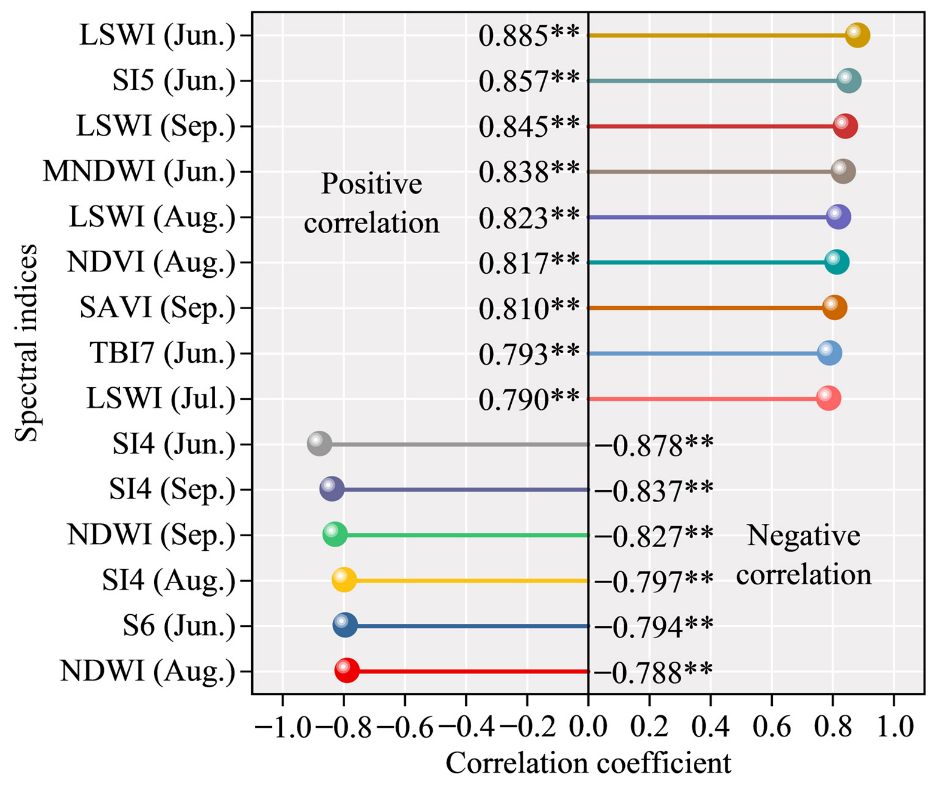
Twenty-five spectral indices from May to October were selected, generating 150 index–month combinations for point-biserial correlation analysis. Combinations were ranked by correlation magnitude (|r|), with the top 15 shown in Figure 3. The top-ranked combinations showed strong correlations (|r| > 0.75, p < 0.01), including nine positive (e.g., June LSWI) and six negative correlations (e.g., June SI4). June dominated among the spectral responses, constituting 60% of top-ranked combinations (9/15), including the top three. This pattern aligns with regional rice farming practices. Post-conversion paddies exhibit pronounced surface transformation during flooding stages. June’s enhanced water–land contrast in remote sensing imagery is optimally acquired by moisture-sensitive (LSWI) and salinity-sensitive (SI4) indices. Albedo variations peak in May and June during the conversion of saline–alkaline land into paddy fields [4]. Therefore, spectral indices during the May–June phase are most likely to reflect the dramatic changes associated with the conversion process. Vegetation indices (August NDVI: rank 9; September SAVI: rank 10) showed lower sensitivity, potentially due to early-stage rice growth constrained by residual salinity and low SOM, reducing spectral contrast with pre-conversion baselines [71]. The vegetation indices gradually increased with time, reflecting vegetation recovery. However, this also reduced their sensitivity to acquiring the abrupt changes associated with the short-term conversion of saline–alkaline land into paddy fields.

By analyzing the pre-/post-conversion differences in spectral indices, the results revealed highly significant variations across all indices. As shown in

Table 3. Statistically significant analysis of spectral indices before and after the conversion.

Spectral Indices	Conversion	Mean Value	Standard Deviation	Absolute Value of Difference	Cohen’s d
SI4 (Jun.)	0	1.147	0.197	0.719 p < 0.001 ***	3.822
	1	0.428	0.171
SI4 (Sep.)	0	1.128	0.209	0.601 p < 0.001 ***	3.179
	1	0.527	0.148
SI5 (Jun.)	0	−0.307	0.113	0.518 p < 0.001 ***	3.476
	1	0.211	0.198
SI4 (Aug.)	0	0.902	0.218	0.512 p < 0.001 ***	2.770
	1	0.39	0.094
MNDWI (Jun.)	0	−0.254	0.112	0.480 p < 0.001 ***	3.197
	1	0.226	0.201
LSWI (Jun.)	0	−0.057	0.11	0.476 p < 0.001 ***	3.972
	1	0.419	0.136
NDVI (Aug.)	0	0.330	0.141	0.401 p < 0.001 ***	2.969
	1	0.731	0.123
LSWI (Aug.)	0	0.071	0.14	0.374 p < 0.001 ***	3.038
	1	0.445	0.084
LSWI (Sep.)	0	−0.048	0.115	0.370 p < 0.001 ***	3.282
	1	0.322	0.109
LSWI (Jul.)	0	0.053	0.154	0.360 p < 0.001 ***	2.683
	1	0.413	0.088
NDWI (Aug.)	0	−0.356	0.115	0.296 p < 0.001 ***	2.683
	1	−0.652	0.101
NDWI (Sep.)	0	−0.293	0.09	0.260 p < 0.001 ***	3.050
	1	−0.553	0.075
SAVI (Sep.)	0	0.150	0.057	0.203 p < 0.001 ***	2.868
	1	0.353	0.09
S6 (Jun.)	0	0.335	0.072	0.179 p < 0.001 ***	2.726
	1	0.156	0.053
TBI7 (Jun.)	0	−0.120	0.062	0.143 p < 0.001 ***	2.715
	1	0.023	0.028

Note: 0 represents before conversion, and 1 represents after conversion (*** represents significance level of 0.001).

, based on the absolute values of the differences before and after the conversion, SI4 in June had the largest difference at 0.719, while TBI7 in June had the smallest difference at 0.143. The Cohen’s d values ranged from 2.683 to 3.972, indicating large effect sizes and very strong separability between converted and unconverted samples for all selected spectral indices. These significant changes in spectral indices highlight the pronounced alterations in surface characteristics caused by the conversion.

3.2. Accuracy Evaluation of Mk Test Detection Results

The MK test implemented on the GEE cloud platform detected the saline–paddy field conversion. The accuracy of different spectral indices was evaluated using field data to determine the detection performance, and the top ten results are presented in

Table 4. Accuracy evaluation of MK tests in detecting saline–alkaline land conversion to paddy fields using different spectral indices.

Spectral Indices	PA (%)	UA (%)	OA (%)	KC
SI5 (Jun.)	94.23	87.50	94.15	0.86
MNDWI (Jun.)	94.00	83.93	92.98	0.84
SI4 (Jun.)	90.20	82.14	91.23	0.76
TBI7 (Jun.)	90.00	80.36	90.64	0.78
LSWI (Jun.)	86.79	82.14	90.06	0.77
LSWI (Jul.)	88.24	78.95	89.53	0.76
SI4 (Sep.)	83.93	83.93	89.47	0.76
SI4 (Aug.)	83.33	80.36	88.30	0.73
LSWI (Sep.)	86.96	71.43	87.13	0.69
LSWI (Aug.)	94.59	62.50	86.55	0.67

. The OAs of the spectral indices varied from 94.15% to 86.55%, the KCs ranged from 0.86 to 0.67, the PAs ranged from 94.59% to 83.33%, and the UAs ranged from 87.50% to 62.50%. Among them, the salinity correlation index SI5 exhibited the highest detection accuracy in June, with an OA of 94.15% and a KC of 0.86. Therefore, it was selected as the optimal index for subsequent mapping. Rice cultivation with phosphogypsum amendment (30 t/ha) significantly reduces soil pH from 10.14 to 8.47 and soil EC from 1092.75 μS·cm⁻¹ to 642.75 μS·cm⁻¹ [72]. Since salinity indices can effectively characterize changes in soil salinity before and after conversion, they demonstrate high detection accuracy in monitoring the conversion of saline–alkaline land into paddy fields. Among these indices, the salinity index SI4 ranked among the top three, achieving an OA of 91.23% and a KC of 0.76. Due to the surface characteristics of the paddy fields during the flooding period, the water body index MNDWI displays stronger sensitivity to flooding signals compared with NDWI and LSWI, having higher detection accuracy in rice mapping [73]. Consequently, MNDWI ranked second, with an OA of 92.98% and a KC of 0.84.

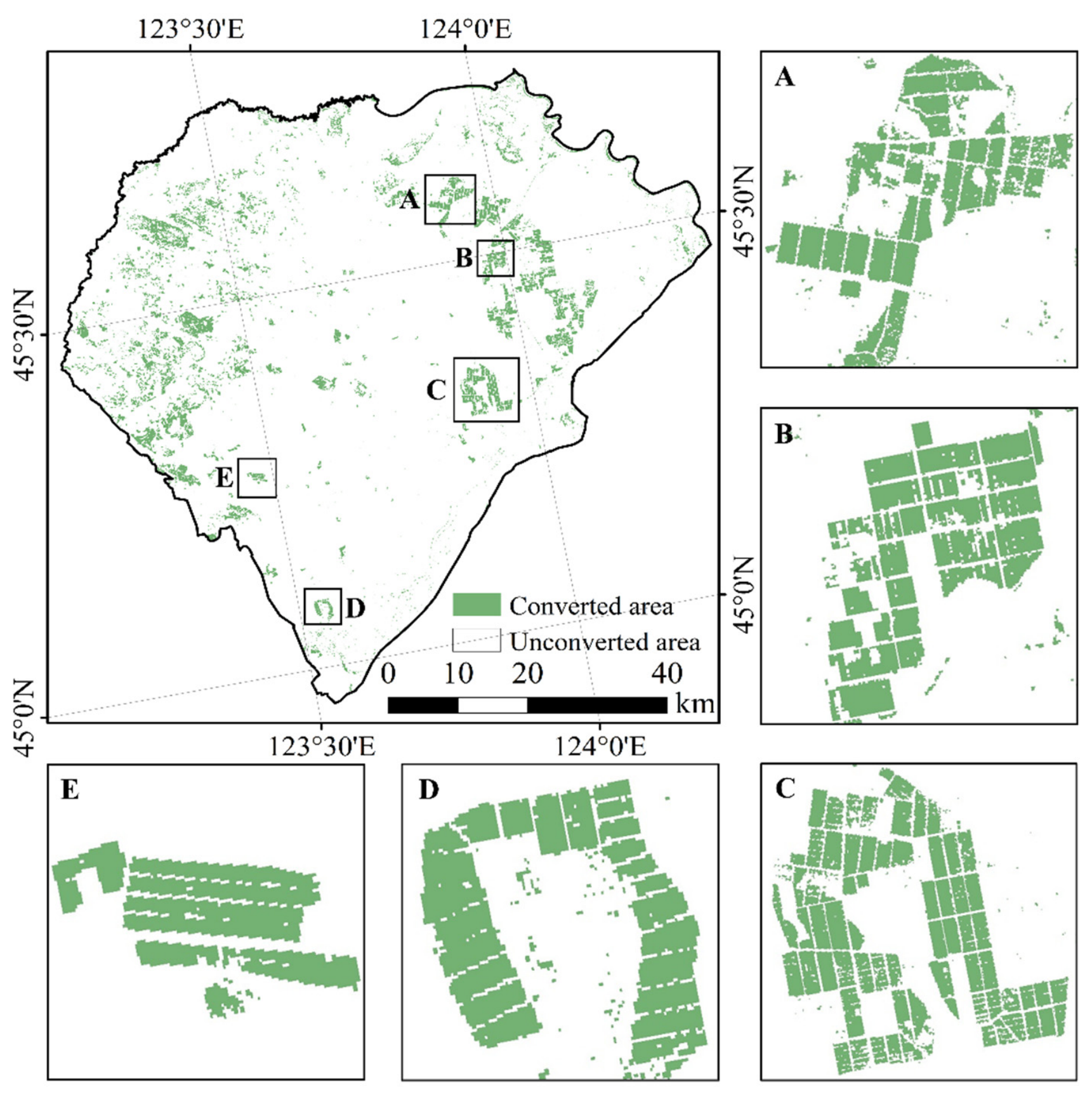
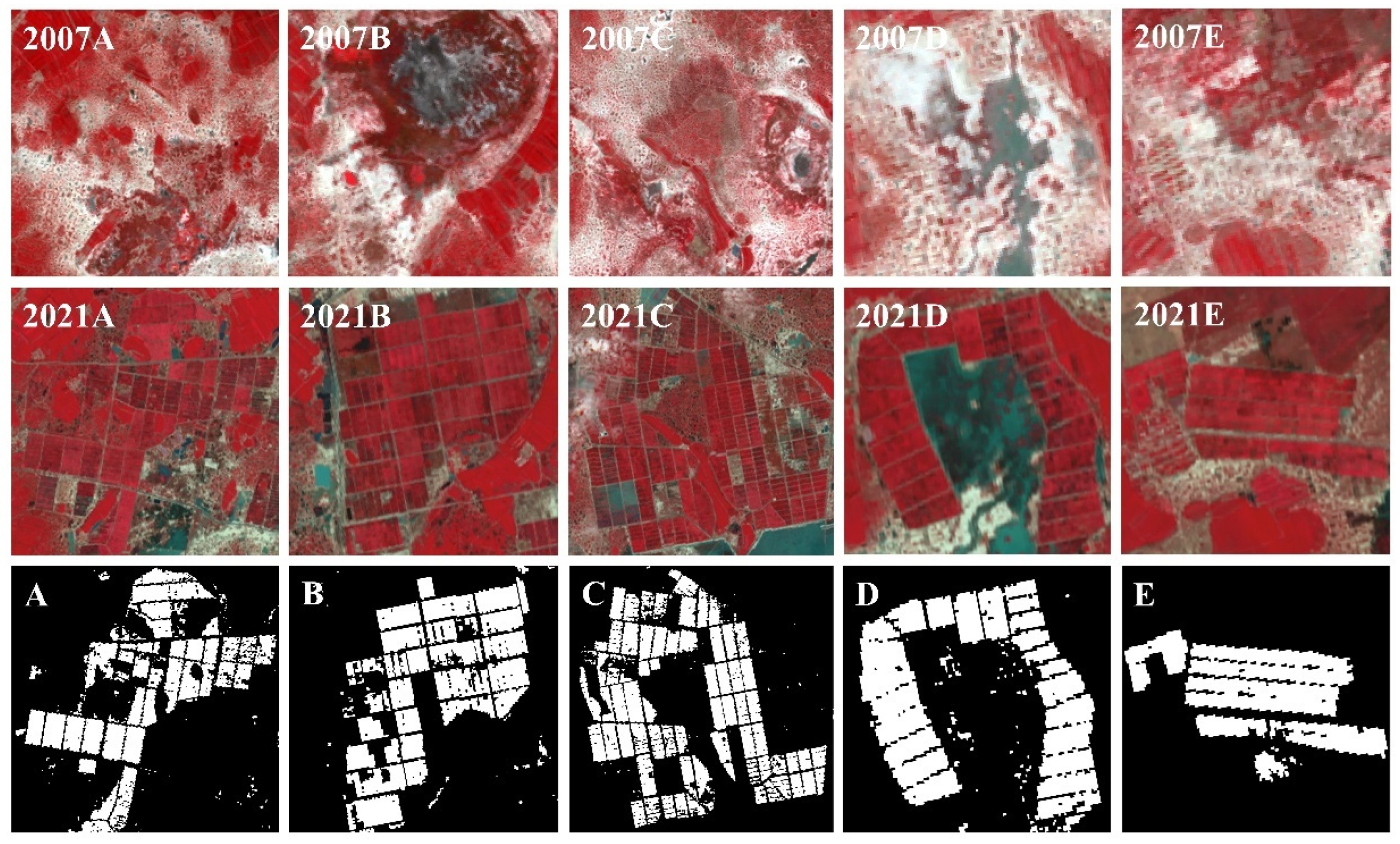
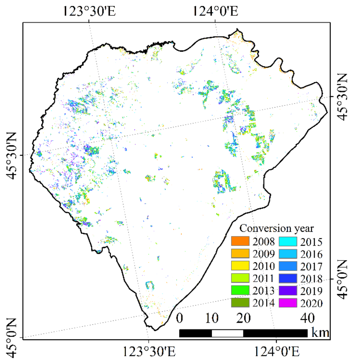
The MK trend analysis, based on June SI5 time-series data (2007–2021), revealed distinct spatial patterns in saline–paddy field conversion (Figure 4). The spatial analysis identified that the majority of conversions clustered in the eastern and western regions, with central regions showing negligible change. Zones A–C in Figure 4 represent eastern conversion zones, which display relatively regular geometric patterns, whereas Zones D–E represent western conversion zones with more irregular field configurations. These patterns highlight the spatial heterogeneity in conversion processes. Furthermore, spatial autocorrelation analysis confirmed stronger clustering in the eastern sectors. In the eastern region, paddy fields were clustered, forming large and contiguous areas. In contrast, the spatial distribution of converted paddy fields in the western region is relatively dispersed. Although this study did not directly quantify irrigation accessibility for each converted field, existing information on regional irrigation infrastructure provides a plausible explanation for this spatial contrast. This disparity may be related to the completion and operation of the Da’an irrigation area water conservancy facility in the eastern part of Da’an City in 2008. The Nenjiang River-derived irrigation system delivers 0.91 × 10⁸ m³/year through 128 km of primary canals, supporting 5.07 × 10⁴ ha paddies [74]. Additionally, the stable water source of the facility minimizes the influence of seasonal rainfall and groundwater fluctuations, thus guaranteeing a reliable water supply during the growing season [75]. Furthermore, once a canal system is constructed, its maintenance costs and energy consumption are lower than those of well-based irrigation systems, rendering it especially suitable for large-scale agricultural production and offering considerable economies of scale [76]. However, paddy fields in the western region are predominantly managed by smallholder farmers, with irrigation water sourced primarily from groundwater [77]. The depth of groundwater varies considerably across different fields in the study area, ranging from 32 m to 90 m, leading to differences in the ease of water access [78]. Well water is highly susceptible to groundwater levels, and water availability may be insufficient during high-demand periods, such as the booting and flowering stages of rice or in cases of over-extraction [79]. The spatial heterogeneity in irrigation conditions in the western region poses challenges in developing large contiguous areas of paddy fields. These conditions may partly explain the more fragmented spatial pattern of converted paddy fields in the western region, but further quantitative analysis of irrigation accessibility is needed to confirm this relationship. Figure 5 illustrates significant changes in surface characteristics before and after the conversion of saline–alkaline land into paddy fields from 2007 to 2021. Prior to conversion, saline–alkaline land was predominantly characterized by bare, high-reflectance areas with low or no vegetation cover. After conversion, these areas were reclaimed as paddy fields with prominent vegetation features.

3.3. Evaluation of Temporal Accuracy and Calculation of Conversion Area

In this study, the timing of saline land conversion to paddy fields in Da’an City from 2007 to 2021 was assessed using the cumulative sum (CUSUM) curve analysis method in conjunction with the MK mutation test, based on the salinity index SI5 time-series data collected each June. As illustrated in Figure 6, the conversion times varied across different fields. This variability may be attributable to differences in the year of conversion or variations in initial soil salinity levels, resulting in inconsistencies in rice growth. Due to the discontinuation of Landsat 5 in 2011 and the launch of Landsat 8 in 2013, no satellite imagery was available for 2012 to contribute to change detection. As shown in

Table 5. Temporal accuracy of conversion detection using the MK mutation test.

Detection Results	Number	Percentage
Correct year	45	80.36%
Temporal discordances	11	19.64%

, the MK mutation test demonstrated an accuracy rate of 80.36% in accurately detecting conversion times in this study. Similarly, Hu et al. [80] used the LandTrendr algorithm to segment Landsat monthly time-series data, successfully determining the construction time of buildings in Beijing. Their study utilized a validation dataset comprising 560 randomly selected building samples, achieving a temporal accuracy of 82.32%. Collectively, these studies underscore the robust capability of time-series-based algorithms in detecting change points across diverse domains.

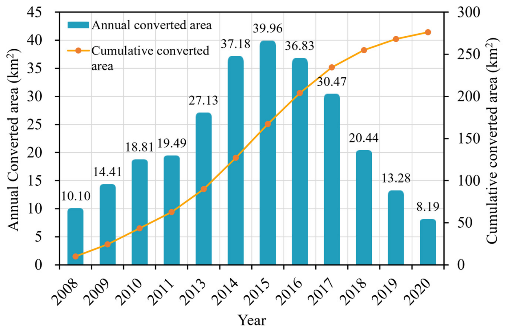
The annual area of saline–alkaline land converted into paddy fields was calculated using the Calculate Geometry tool in ArcGIS 10.8, with spatiotemporal dynamics visualized in Figure 7. As shown in Figure 7, the conversion area in Da’an City exhibited an initial increase, followed by a gradual decline. The annual conversion area increased steadily from 10.1 km² in 2008, peaking at 39.96 km² in 2015, and then gradually decreasing to 8.19 km² in 2020. The cumulative reclamation reached 276.29 km² (2008–2020), with 2014–2017 accounting for 52.28% of the total transition. Long-term agroecological trials by Lu et al. [72] demonstrated the synergistic effects of phosphogypsum-amended rice systems, enhancing sodicity reduction by 38.89% and yield augmentation by 25–50% over 5-year cycles. This system’s adoption was catalyzed by dual innovations in 2015: (1) scaling soil amendment protocols for saline–sodic landscapes [72]; (2) the release of ‘Dongdao-4’—a salt-tolerant rice cultivar with 8.02 t/ha potential yield [81]. These advancements significantly accelerated saline–alkaline land reclamation efforts, resulting in the highest recorded conversion area in 2015. However, saline–alkaline land near irrigation canals was prioritized for conversion, as reclamation is simpler and less costly. In contrast, areas farther from irrigation canals face higher reclamation costs, and the marginal returns decrease considerably, likely explaining the declining annual conversion area after 2015 [82]. Xin et al. [26] applied an object-oriented classification algorithm coupled with a bi-temporal change detection method to map 2015–2021 LULC transitions, reporting 76.06 km² conversions in this study area. In comparison, the conversion area during the same period in this study was 109.21 km². This 30.5% discrepancy (109.21 km² vs. 76.06 km²) may stem from bi-temporal change detection classification accumulating errors from both datasets [13]. Furthermore, the spectral similarities between saline–alkaline land and grassland can reduce classification precision [27]. In western Jilin Province, 45.22% of the expansion of saline–alkaline land was attributed to grassland degradation [83]. In remote sensing imagery, mild and moderate saline–alkaline land often appear as patches of vegetation, increasing the probability of misclassification during visual interpretation. Thus, mild and moderate saline–alkaline land may be misclassified as grassland during classification, leading to the erroneous calculation of paddy fields reclaimed from saline–alkaline land as conversions from grassland.

4. Discussion

4.1. Detection Capabilities of Mk Trend and Mutation Tests

On a large scale, the conversion of saline–alkaline land into paddy fields is a long-term process accompanied by substantial surface changes. Conventional bi-temporal approaches fail to capture gradual transitions, as they only compare discrete snapshots (e.g., 2000 vs. 2020) without characterizing interim dynamics [84]. Therefore, time-series detection offers a more effective approach to monitoring these extended periods of change [15]. However, policy and cost constraints can lead to the abandonment of certain paddy fields, potentially leading to false detections [85]. This study employed a two-stage detection to avoid the impact of fallowed fields: (1) MK trend test (α = 0.05) for conversion occurrence; (2) mutation analysis for temporal pinpointing. Trend and change-point detection provide a suitable basis for identifying both the occurrence and timing of saline–alkaline land conversion from remote-sensing time series [11]. Numerous trend and change-point detection algorithms have been proposed and applied in farmland change detection [8]. Zhu et al. [86] achieved 87.0% OA for farmland–lake transitions using LandTrendr; however, this required annual NDVI composites (May–September) as preconditioning inputs. Similarly, Xu et al. [87] applied the CCDC algorithm to analyze cropland abandonment from 1986 to 2021 in Yibin City, China. The validation results from stratified random samples revealed that the temporal accuracy in detecting abandoned farmland ranged from 43% to 71%. Both methods rely on farmland extraction, either using the Random Forest classifier or combining multiple land-cover products, limiting the change detection accuracy because of reduced classification accuracy. The MK-based framework achieved an overall accuracy of 94.15% without requiring annual land-cover pre-classification, which may reduce the potential propagation of classification errors commonly associated with classifier-dependent change detection approaches. This demonstrates that the MK trend test is an effective method for detecting dynamic changes in the conversion process, but its relative advantage over other methods requires further validation through controlled comparisons. Comparative analysis showed MK’s superiority: an 8.2% higher F1-score than modified MK and 15.7% higher than Cox–Stuart in non-normal distributions [88]. In addition, it displayed higher detection accuracies and lower false detection rates, rendering it more advantageous for mutation detection. Moreover, for fixed-length time series, the trend detection capability of the MK test increases as the slope steepens [23]. To enhance the performance of the MK test in this study, optimal index–month selection improved detection precision and accuracy.

Accurate information on change detection in farmland and other land use is crucial for environmental assessment and policy formulation. Mardian et al. [89] employed the BFAST algorithm to detect the conversion of rangelands and pastures to farmland using MODIS and Landsat data. The validation results demonstrated that the temporal accuracy metrics for monitoring the conversion of rangelands and pastures to farmland were 76% and 66%, respectively. Wang et al. [90] proposed a graph-based segmentation for a multivariate time-series algorithm (MTS-GS) and applied this method to detect urban changes in Luoyang City, China, using Sentinel-2 time-series data. The validation results based on high-spatial-resolution imagery from Google Earth indicated a temporal accuracy of 81.8%. However, their inherent sensitivity to the revisit time of remote sensing data renders these two methods better suited for small-scale change detection, such as in pastures or urban neighborhoods, and they exhibit limited effectiveness for large-scale applications [89,90]. In this study, the MK test exhibited strong robustness in detecting the conversion of saline–alkaline land to paddy fields because of its nonparametric nature and reduced sensitivity to outliers. Its temporal accuracy reached 80.36%. The temporal accuracies reported for CCDC, BFAST, and MTS-GS in the studies cited above are used only as background references because they were obtained from different datasets, study areas, environmental conditions, and validation designs. They do not constitute a controlled comparison with this study. This performance is primarily attributable to the varying degree of salinization in saline–alkaline land, leading to significant differences in rice growth conditions and yields among converted fields. In paddy fields converted from severely saline–alkaline land, rice failed to establish and grow in the first year after conversion [25]. Consequently, these fields retained the spectral characteristics of saline–alkaline land in remote sensing imagery, thus compromising temporal detection accuracy. In the past two decades, the breeding of salt-tolerant rice varieties has progressed rapidly, and the salt-tolerance performance of rice varieties planted across years has varied notably, also impacting the detection accuracy [91].

4.2. The Influence of Wetlands and Water Bodies on the Results

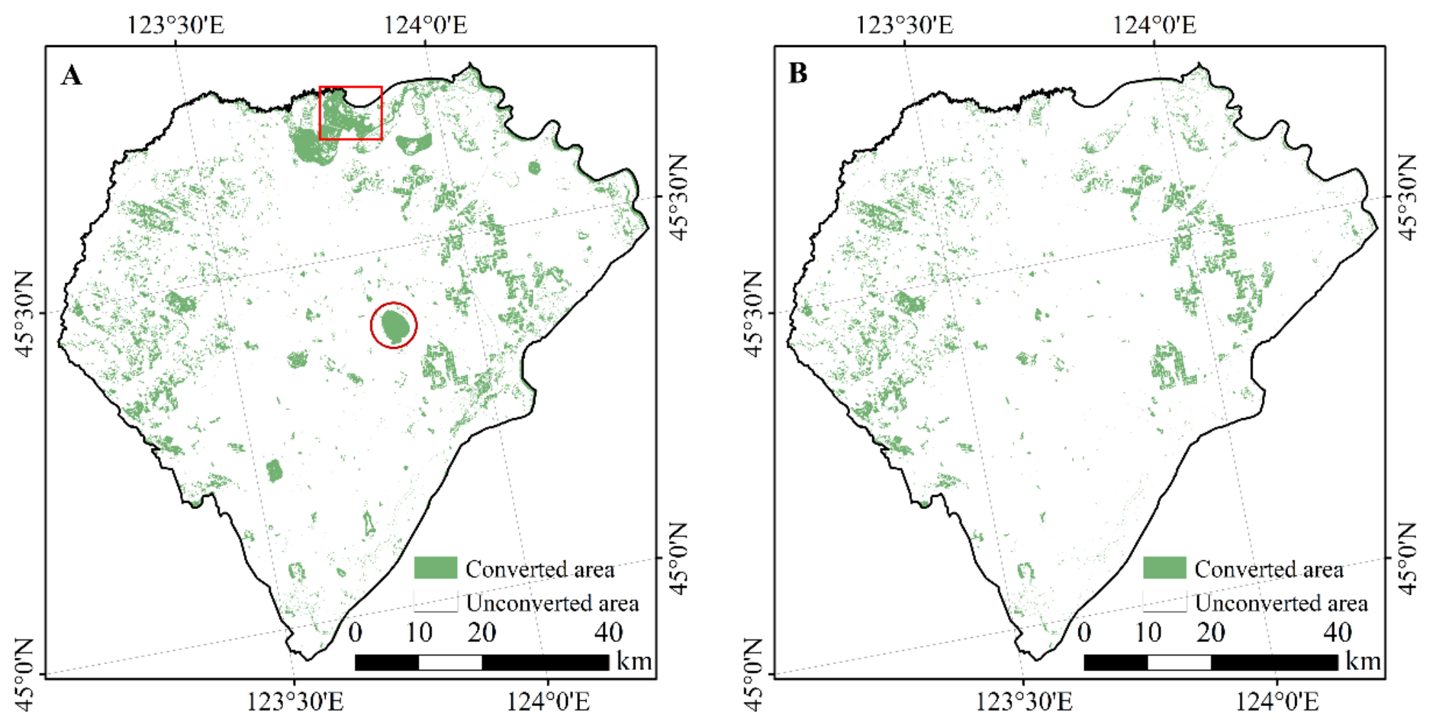
Single-temporal mapping frameworks encounter inherent challenges in resolving the spectral ambiguities between ephemeral wetlands and flooded paddies [31]. Regional variations in climatic conditions and cropping patterns can result in spatially heterogeneous impacts of wetland features and their dynamics on rice mapping accuracy [92]. Therefore, mitigating wetland-induced interference in the MK detection results becomes imperative. This research used the global 30-m annual wetland dataset (GWL_FCS30D) from 2017 to 2021 to decouple wetland dynamics from MK trend analysis.

Significant spectral similarity exists between flooded paddy fields and open water bodies during the pre-transplantation stage [36]. This spectral overlap may lead to classification inaccuracies when monitoring land cover transitions from saline land to paddies. As a robust adaptive thresholding method, the Otsu algorithm has been extensively utilized for aquatic feature delineation in remote sensing applications [65]. In this study, to mitigate hydrological interference, we implemented the Otsu algorithm for 2007–2021 spring water body delineation. The classification achieved 92.86% OA, with a KC of 0.86 (Table S1). This study applied spatial masking procedures using annual wetland–water body data to isolate their confounding effects. Comparative analysis of MK trend maps (Figure 8) reveals distinct patterns: baseline results are shown without wetland–water body exclusion (Panel A) versus refined outputs post-masking (Panel B). A comparison between these panels highlights that wetlands and water bodies had a significant impact on the detection results, particularly in the northern and central regions of the study area where these features are concentrated. Yueliangpao Lake and Xiaoxinmipao Lake provide representative examples of hydrological changes that could be misidentified as saline–alkaline-to-paddy conversion. Yueliangpao Lake in the northern area of Da’an City, which is an important flood management infrastructure, exhibited 21.25 km² of cumulative expansion [93]. Similarly, hydrological regime shifts transformed Xiaoxinmipao Lake from a seasonal to a perennial status post-2013 [94]. The salinity index variations observed in these regions predominantly originated from wetland-aquatic system dynamics rather than saline–alkaline land conversion. The quantitative accuracy assessment (

Table 6. Comparison of MK test detection accuracy before and after wetland and water body masking.

SI5 (Jun.)	PA (%)	UA (%)	OA (%)	KC
Unremoved wetlands and water bodies	69.01	87.50	83.04	0.64
Removed wetlands and water bodies	94.23	87.50	94.15	0.86

) demonstrated wetland-induced MK classification degradation: the PA declined by 23.15% (92.86% → 69.01%) when retaining aquatic features. This interference decreased the OA by 11.11% (94.15% → 83.04%) and KC by 0.22. Masking implementation restored classification fidelity to 94.15% (Δ + 11.11%) with KC = 0.86, conclusively demonstrating that wetland-aquatic dynamics can induce >10% analytical bias and necessitating systematic hydrological correction in land conversion monitoring.

4.3. Shortcomings and Future Prospects

This study employed the MK test to quantify the spatiotemporal dynamics of saline–paddy field conversion through three analytical dimensions: trend magnitude (S), persistence (p < 0.05), and mutation certainty (CUSUM threshold = ±2σ). Dissimilar to classifier-dependent methods (CCDC and BFAST), the MK framework achieved 94.15% accuracy without land cover pre-classification by integrating rice phenology. However, applying the MK trend test for conversion monitoring necessitates careful determination of threshold values to ensure high-accuracy detection. Threshold determination demands prior knowledge, thus constraining the generalizability of this test [95]. Sun et al. [96] developed adaptive CVA thresholds using spectral divergence indices (SDI > 0.23), achieving 91.80% accuracy in arid land transitions. Previous studies suggest that adaptive thresholding may improve change detection, but its transferability to saline–alkaline land conversion remains untested. Furthermore, certain agricultural fields in the detection results exhibited incompleteness, accompanied by a salt-and-pepper phenomenon, indicating temporal inconsistencies in land conversion within individual fields. The neighbor mapping and manifold projection (NM_MP) algorithm improved edge coherence by 38% and reduced speckle noise (ENL = 15.2 vs. 8.7 baseline) in agricultural landscapes [97]. Future work should explore object-based refinement or spatial-consistency post-processing to reduce salt-and-pepper noise and improve the completeness of field-level conversion mapping. A methodological integration of change consistency checks with object-based reclassification should be implemented to address these limitations. This approach aims to enhance the spatial coherence of land use change detection while systematically mitigating the salt-and-pepper phenomenon attributable to stochastic noise [98].

Compared with seasonal wetlands, permanent wetlands exhibit stable distributions and minimal variation in terms of their spectral characteristics, facilitating the exclusion of their interference during change detection [88]. Meteorological records from the past decade indicate that precipitation in Da’an City is concentrated in July and August, with rainfall in June amounting to 65 mm, constituting 12.5% of the annual total [99]. Therefore, seasonal wetlands resulting from precipitation may compromise change detection results derived from June time-series remote sensing data. Future research should prioritize the application of the temporal–spectral–semantic-aware convolutional transformer network (TSSA-CTNet) for seasonal wetland extraction, thus improving the accuracy and regional applicability of change detection [100].

5. Conclusions

The strategic conversion of saline–alkaline lands into productive paddies plays an important role in addressing global food security challenges while advancing SDG 15.3 (land degradation neutrality). This study developed an MK-based time-series framework using Landsat data to monitor the spatiotemporal dynamics of the conversion of saline–alkaline land to paddy fields in Da’an City from 2007 to 2021.

The results show that salinity-related spectral indices can effectively capture the surface changes associated with this land conversion process. Among the tested indices, the June SI5 salinity index showed the best performance in identifying converted areas. The MK trend and mutation tests further enabled the identification of conversion occurrence and timing, while the detected conversions exhibited clear spatial and temporal heterogeneity. Spatially, converted paddy fields were mainly distributed in the eastern and western parts of Da’an City, with relatively limited conversion in the central region. Temporally, the conversion process underwent an expansion phase followed by a gradual decline and showed distinct stage-wise variation.

Despite its effectiveness, the proposed framework still has limitations related to threshold selection, wetland and water-body interference, salt-and-pepper noise, and uncertainty in conversion-year detection. Future studies should further improve field-level mapping through object-based refinement and spatial-consistency post-processing, while refining wetland and water-body masking to reduce false detections.

References

1. Chen, L.; Zhou, G.; Feng, B.; Wang, C.; Luo, Y.; Li, F.; Shen, C.; Ma, D.; Zhang, C.; Zhang, J. Saline-Alkali Land Reclamation Boosts Topsoil Carbon Storage by Preferentially Accumulating Plant-Derived Carbon. Sci. Bull. 2024, 69, 2948–2958. [Google Scholar] [CrossRef] [PubMed]
2. Liu, L.; Wang, B. Protection of Halophytes and Their Uses for Cultivation of Saline-Alkali Soil in China. Biology 2021, 10, 353. [Google Scholar] [CrossRef] [PubMed]
3. Qi, P.; Li, B.; Zhang, D.; Xu, H.; Zhang, G. Supply and Demand of Agricultural Water Resources under Future Saline-Alkali Land Improvement. Agric. Water Manag. 2025, 314, 109503. [Google Scholar] [CrossRef]
4. Yu, L.; Yang, J.; Bu, K.; Liu, T.; Jiao, Y.; Li, G.; Pu, L.; Zhang, S. Impacts of Saline-Alkali Land Improvement on Regional Climate: Process, Mechanisms, and Implications. Remote Sens. 2021, 13, 3407. [Google Scholar] [CrossRef]
5. Talukdar, S.; Singha, P.; Mahato, S.; Shahfahad; Pal, S.; Liou, Y.-A.; Rahman, A. Land-Use Land-Cover Classification by Machine Learning Classifiers for Satellite Observations—A Review. Remote Sens. 2020, 12, 1135. [Google Scholar] [CrossRef]
6. Sahbeni, G.; Ngabire, M.; Musyimi, P.K.; Székely, B. Challenges and Opportunities in Remote Sensing for Soil Salinization Mapping and Monitoring: A Review. Remote Sens. 2023, 15, 2540. [Google Scholar] [CrossRef]
7. Wang, J.; Zhen, J.; Hu, W.; Chen, S.; Lizaga, I.; Zeraatpisheh, M.; Yang, X. Remote Sensing of Soil Degradation: Progress and Perspective. Int. Soil Water Conserv. Res. 2023, 11, 429–454. [Google Scholar] [CrossRef]
8. Chughtai, A.H.; Abbasi, H.; Karas, I.R. A Review on Change Detection Method and Accuracy Assessment for Land Use Land Cover. Remote Sens. Appl. Soc. Environ. 2021, 22, 100482. [Google Scholar] [CrossRef]
9. Jiao, W.; Wang, L.; McCabe, M.F. Multi-Sensor Remote Sensing for Drought Characterization: Current Status, Opportunities and a Roadmap for the Future. Remote Sens. Environ. 2021, 256, 112313. [Google Scholar] [CrossRef]
10. Wang, X.; Du, P.; Liu, S.; Senyshen, M.; Zhang, W.; Fang, H.; Fan, X. A Novel Multiple Change Detection Approach Based on Tri-Temporal Logic-Verified Change Vector Analysis in Posterior Probability Space. Int. J. Appl. Earth Obs. Geoinf. 2022, 111, 102852. [Google Scholar] [CrossRef]
11. Zhang, C.; Yue, P.; Tapete, D.; Jiang, L.; Shangguan, B.; Huang, L.; Liu, G. A Deeply Supervised Image Fusion Network for Change Detection in High Resolution Bi-Temporal Remote Sensing Images. ISPRS J. Photogramm. Remote Sens. 2020, 166, 183–200. [Google Scholar] [CrossRef]
12. Demarquet, Q.; Rapinel, S.; Gore, O.; Dufour, S.; Hubert-Moy, L. Continuous Change Detection Outperforms Traditional Post-Classification Change Detection for Long-Term Monitoring of Wetlands. Int. J. Appl. Earth Obs. Geoinf. 2024, 133, 104142. [Google Scholar] [CrossRef]
13. Li, Y.; Li, X.; Song, J.; Wang, Z.; He, Y.; Yang, S. Remote-Sensing-Based Change Detection Using Change Vector Analysis in Posterior Probability Space: A Context-Sensitive Bayesian Network Approach. IEEE J. Sel. Top. Appl. Earth Obs. Remote Sens. 2023, 16, 3198–3217. [Google Scholar] [CrossRef]
14. Kalinicheva, E.; Ienco, D.; Sublime, J.; Trocan, M. Unsupervised Change Detection Analysis in Satellite Image Time Series Using Deep Learning Combined with Graph-Based Approaches. IEEE J. Sel. Top. Appl. Earth Obs. Remote Sens. 2020, 13, 1450–1466. [Google Scholar] [CrossRef]
15. Woodcock, C.E.; Loveland, T.R.; Herold, M.; Bauer, M.E. Transitioning from Change Detection to Monitoring with Remote Sensing: A Paradigm Shift. Remote Sens. Environ. 2020, 238, 111558. [Google Scholar] [CrossRef]
16. Guo, H.; Wang, Y.; Yu, J.; Yi, L.; Shi, Z.; Wang, F. A Novel Framework for Vegetation Change Characterization from Time Series Landsat Images. Environ. Res. 2023, 222, 115379. [Google Scholar] [CrossRef] [PubMed]
17. Verbesselt, J.; Hyndman, R.; Newnham, G.; Culvenor, D. Detecting Trend and Seasonal Changes in Satellite Image Time Series. Remote Sens. Environ. 2010, 114, 106–115. [Google Scholar] [CrossRef]
18. Yan, J.; Wang, L.; Song, W.; Chen, Y.; Chen, X.; Deng, Z. A Time-Series Classification Approach Based on Change Detection for Rapid Land Cover Mapping. ISPRS J. Photogramm. Remote Sens. 2019, 158, 249–262. [Google Scholar] [CrossRef]
19. Kennedy, R.; Yang, Z.; Cohen, W. Detecting Trends in Forest Disturbance and Recovery Using Yearly Landsat Time Series: 1. LandTrendr—Temporal Segmentation Algorithms. Remote Sens. Environ. 2010, 114, 2897–2910. [Google Scholar] [CrossRef]
20. Pasquarella, V.J.; Arévalo, P.; Bratley, K.H.; Bullock, E.L.; Gorelick, N.; Yang, Z.; Kennedy, R.E. Demystifying LandTrendr and CCDC Temporal Segmentation. Int. J. Appl. Earth Obs. Geoinf. 2022, 110, 102806. [Google Scholar] [CrossRef]
21. Zhu, Z.; Woodcock, C.E. Continuous Change Detection and Classification of Land Cover Using All Available Landsat Data. Remote Sens. Environ. 2014, 144, 152–171. [Google Scholar] [CrossRef]
22. Brown, J.F.; Tollerud, H.J.; Barber, C.P.; Zhou, Q.; Dwyer, J.L.; Vogelmann, J.E.; Loveland, T.R.; Woodcock, C.E.; Stehman, S.V.; Zhu, Z.; et al. Lessons Learned Implementing an Operational Continuous United States National Land Change Monitoring Capability: The Land Change Monitoring, Assessment, and Projection (LCMAP) Approach. Remote Sens. Environ. 2020, 238, 111356. [Google Scholar] [CrossRef]
23. Wang, F.; Shao, W.; Yu, H.; Kan, G.; He, X.; Zhang, D.; Ren, M.; Wang, G. Re-Evaluation of the Power of the Mann-Kendall Test for Detecting Monotonic Trends in Hydrometeorological Time Series. Front. Earth Sci. 2020, 8, 14. [Google Scholar] [CrossRef]
24. Hu, J.; Ye, B.; Bai, Z.; Feng, Y. Remote Sensing Monitoring of Vegetation Reclamation in the Antaibao Open-Pit Mine. Remote Sens. 2022, 14, 5634. [Google Scholar] [CrossRef]
25. Li, X.; Li, Y.; Wang, B.; Sun, Y.; Cui, G.; Liang, Z. Analysis of Spatial-Temporal Variation of the Saline-Sodic Soil in the West of Jilin Province from 1989 to 2019 and Influencing Factors. Catena 2022, 217, 106492. [Google Scholar] [CrossRef]
26. Xin, B.; Yu, L.; Li, G.; Jiao, Y.; Liu, T.; Zhang, S.; Lei, Z. Impact of Saline-Alkali Land Greening on the Local Surface Temperature—A Multiscale Assessment Based on Remote Sensing. Remote Sens. 2022, 14, 4246. [Google Scholar] [CrossRef]
27. Cao, Y.; Hou, G.; Chen, Z.; Gong, Y.; Zhou, J.; Liu, Z. Quantitative Determination of the Optimal Scale for the Proportion of Saline-Alkali Patches of Soda Saline-Alkali Land in Northeast China. IEEE J. Sel. Top. Appl. Earth Obs. Remote Sens. 2024, 17, 5378–5389. [Google Scholar] [CrossRef]
28. Gu, Z.; Bian, J.; Wu, J.; Ruan, D.; Yu, Y.; Zhang, H. Effects of Anthropogenic Activities on Hydrochemical Characteristics of Ground Water of Da’an Irrigation Area in Western of Jilin Province. Environ. Sci. Pollut. Res. 2022, 29, 20479–20495. [Google Scholar] [CrossRef] [PubMed]
29. Li, C.; Jin, S. Aligning Legacy NLCD Land Cover Maps Based on Landsat Collection 1 to Collection 2. Int. J. Appl. Earth Obs. Geoinf. 2026, 149, 105314. [Google Scholar] [CrossRef]
30. Yang, J.; Huang, X. The 30 m Annual Land Cover Dataset and Its Dynamics in China from 1990 to 2019. Earth Syst. Sci. Data 2021, 13, 3907–3925. [Google Scholar] [CrossRef]
31. Lin, S.; Qi, Z.; Li, X.; Zhang, H.; Lv, Q.; Huang, D. A Phenological-Knowledge-Independent Method for Automatic Paddy Rice Mapping with Time Series of Polarimetric SAR Images. ISPRS J. Photogramm. Remote Sens. 2024, 218, 628–644. [Google Scholar] [CrossRef]
32. Zhang, X.; Liu, L.; Zhao, T.; Wang, J.; Liu, W.; Chen, X. Global Annual Wetland Dataset at 30 m with a Fine Classification System from 2000 to 2022. Sci. Data 2024, 11, 310. [Google Scholar] [CrossRef] [PubMed]
33. Huang, L.; Liu, Y.; Ferreira, J.F.S.; Wang, M.; Na, J.; Huang, J.; Liang, Z. Long-Term Combined Effects of Tillage and Rice Cultivation with Phosphogypsum or Farmyard Manure on the Concentration of Salts, Minerals, and Heavy Metals of Saline-Sodic Paddy Fields in Northeast China. Soil Tillage Res. 2022, 215, 105222. [Google Scholar] [CrossRef]
34. Racetin, I.; Krtalic, A.; Srzic, V.; Zovko, M. Characterization of Short-Term Salinity Fluctuations in the Neretva River Delta Situated in the Southern Adriatic Croatia Using Landsat-5 TM. Ecol. Indic. 2020, 110, 105924. [Google Scholar] [CrossRef]
35. Yu, H.; Wang, Z.; Mao, D.; Jia, M.; Chang, S.; Li, X. Spatiotemporal Variations of Soil Salinization in China’s West Songnen Plain. Land Degrad. Dev. 2023, 34, 2366–2378. [Google Scholar] [CrossRef]
36. Xia, L.; Zhao, F.; Chen, J.; Yu, L.; Lu, M.; Yu, Q.; Liang, S.; Fan, L.; Sun, X.; Wu, S.; et al. A Full Resolution Deep Learning Network for Paddy Rice Mapping Using Landsat Data. ISPRS J. Photogramm. Remote Sens. 2022, 194, 91–107. [Google Scholar] [CrossRef]
37. Gopinath, G.; Surendran, U.; Vishak, J.; Sasidharan, N.; Fasil CT, M. Hyperspectral Data and Vegetative Indices for Paddy: A Case Study in Kerala, India. Remote Sens. Appl. Soc. Environ. 2024, 33, 101109. [Google Scholar] [CrossRef]
38. Yang, J.; Hu, Q.; Li, W.; Song, Q.; Cai, Z.; Zhang, X.; Wei, H.; Wu, W. An Automated Sample Generation Method by Integrating Phenology Domain Optical-SAR Features in Rice Cropping Pattern Mapping. Remote Sens. Environ. 2024, 314, 114387. [Google Scholar] [CrossRef]
39. Jiang, R.; Sanchez-Azofeifa, A.; Laakso, K.; Xu, Y.; Zhou, Z.; Luo, X.; Huang, J.; Chen, X.; Zang, Y. Cloud Cover throughout All the Paddy Rice Fields in Guangdong, China: Impacts on Sentinel 2 MSI and Landsat 8 OLI Optical Observations. Remote Sens. 2021, 13, 2961. [Google Scholar] [CrossRef]
40. Tian, J.; Zhu, X.; Chen, J.; Wang, C.; Shen, M.; Yang, W.; Tan, X.; Xu, S.; Li, Z. Improving the Accuracy of Spring Phenology Detection by Optimally Smoothing Satellite Vegetation Index Time Series Based on Local Cloud Frequency. ISPRS J. Photogramm. Remote Sens. 2021, 180, 29–44. [Google Scholar] [CrossRef]
41. Khan, N.M.; Rastoskuev, V.V.; Sato, Y.; Shiozawa, S. Assessment of Hydrosaline Land Degradation by Using a Simple Approach of Remote Sensing Indicators. Agric. Water Manag. 2005, 77, 96–109. [Google Scholar] [CrossRef]
42. Douaoui, A.E.K.; Nicolas, H.; Walter, C. Detecting Salinity Hazards within a Semiarid Context by Means of Combining Soil and Remote-Sensing Data. Geoderma 2006, 134, 217–230. [Google Scholar] [CrossRef]
43. Abderrazak, B.; Guedon, A.; El Harti, A.; Cherkaoui, F.; Abderrahmene, E. Characterization of Slightly and Moderately Saline and Sodic Soils in Irrigated Agricultural Land Using Simulated Data of Advanced Land Imaging (EO-1) Sensor. Commun. Soil Sci. Plant Anal. 2008, 39, 2795–2811. [Google Scholar] [CrossRef]
44. Abbas, A.; Khan, S. Using Remote Sensing Techniques for Appraisal of Irrigated Soil Salinity. In Proceedings of the International Congress on Modelling and Simulation (MODSIM); Modelling and Simulation Society of Australia and New Zealand: Canberra, Australia, 2007; pp. 2632–2638. [Google Scholar]
45. Dehni, A.; Lounis, M. Remote Sensing Techniques for Salt Affected Soil Mapping: Application to the Oran Region of Algeria. Procedia Eng. 2012, 33, 188–198. [Google Scholar] [CrossRef]
46. Scudiero, E.; Skaggs, T.H.; Corwin, D.L. Regional Scale Soil Salinity Evaluation Using Landsat 7, Western San Joaquin Valley, California, USA. Geoderma Reg. 2014, 2, 82–90. [Google Scholar] [CrossRef]
47. Zhou, X.; Zhang, F.; Liu, C.; Kung, H.; Johnson, V.C. Soil Salinity Inversion Based on Novel Spectral Index. Environ. Earth Sci. 2021, 80, 501. [Google Scholar] [CrossRef]
48. Khan, N.; Rastoskuev, V.V.; Shalina, E.; Sato, Y. Mapping Salt-Affected Soils Using Remote Sensing Indicators-a Simple Approach with the Use of GIS IDRISI; Asian Conference on Remote Sensing: Singapore, 2001. [Google Scholar]
49. Huete, A.; Didan, K.; Miura, T.; Rodriguez, E.P.; Gao, X.; Ferreira, L.G. Overview of the Radiometric and Biophysical Performance of the MODIS Vegetation Indices. Remote Sens. Environ. 2002, 83, 195–213. [Google Scholar] [CrossRef]
50. Jordan, C.F. Derivation of Leaf-Area Index from Quality of Light on the Forest Floor. Ecology 1969, 50, 663–666. [Google Scholar] [CrossRef]
51. Huete, A.R. A Soil-Adjusted Vegetation Index (SAVI). Remote Sens. Environ. 1988, 25, 295–309. [Google Scholar] [CrossRef]
52. Chandrasekar, K.; Sesha Sai, M.V.R.; Roy, P.S.; Dwevedi, R.S. Land Surface Water Index (LSWI) Response to Rainfall and NDVI Using the MODIS Vegetation Index Product. Int. J. Remote Sens. 2010, 31, 3987–4005. [Google Scholar] [CrossRef]
53. Gao, B. NDWI—A Normalized Difference Water Index for Remote Sensing of Vegetation Liquid Water from Space. Remote Sens. Environ. 1996, 58, 257–266. [Google Scholar] [CrossRef]
54. Xu, H. Modification of Normalised Difference Water Index (NDWI) to Enhance Open Water Features in Remotely Sensed Imagery. Int. J. Remote Sens. 2006, 27, 3025–3033. [Google Scholar] [CrossRef]
55. Shang, Y.; Song, K.; Lai, F.; Lyu, L.; Liu, G.; Fang, C.; Hou, J.; Qiang, S.; Yu, X.; Wen, Z. Remote Sensing of Fluorescent Humification Levels and Its Potential Environmental Linkages in Lakes across China. Water Res. 2023, 230, 119540. [Google Scholar] [CrossRef] [PubMed]
56. Zhang, D.; Hu, B.; Chen, L.; Qi, P.; Wu, Y.; Liu, X.; Zhang, G.; Zhang, W. Spatiotemporal Variation of Water Level in Wetlands Based on Multi-Source Remote Sensing Data and Responses to Changing Environments. Sci. Total Environ. 2024, 955, 177060. [Google Scholar] [CrossRef] [PubMed]
57. Esterhuizen, H.J.; Slippers, B.; Bosman, A.S.; Roux, J.; Jones, W.; Bose, T.; Hammerbacher, A. Early Detection of Phytophthora Root Rot in Eucalyptus Using Hyperspectral Reflectance and Machine Learning. Comput. Electron. Agric. 2025, 237, 110761. [Google Scholar] [CrossRef]
58. Zhang, Y.; Ma, R.; Hu, M.; Luo, J.; Li, J.; Liang, Q. Combining Citizen Science and Land Use Data to Identify Drivers of Eutrophication in the Huangpu River System. Sci. Total Environ. 2017, 584–585, 651–664. [Google Scholar] [CrossRef] [PubMed]
59. Werther, M.; Odermatt, D.; Simis, S.G.H.; Gurlin, D.; Lehmann, M.K.; Kutser, T.; Gupana, R.; Varley, A.; Hunter, P.D.; Tyler, A.N.; et al. A Bayesian Approach for Remote Sensing of Chlorophyll-a and Associated Retrieval Uncertainty in Oligotrophic and Mesotrophic Lakes. Remote Sens. Environ. 2022, 283, 113295. [Google Scholar] [CrossRef]
60. Kendall, M. Rank Correlation Methods; Charles Griffin: Granville, OH, USA, 1975. [Google Scholar]
61. Bai, Y.; Li, S.; Liu, M.; Guo, Q. Assessment of Vegetation Change on the Mongolian Plateau over Three Decades Using Different Remote Sensing Products. J. Environ. Manag. 2022, 317, 115509. [Google Scholar] [CrossRef] [PubMed]
62. Agbo, E.P.; Nkajoe, U.; Edet, C.O. Comparison of Mann–Kendall and Şen’s Innovative Trend Method for Climatic Parameters over Nigeria’s Climatic Zones. Clim. Dyn. 2023, 60, 3385–3401. [Google Scholar] [CrossRef]
63. Otsu, N. A Threshold Selection Method from Gray-Level Histograms. IEEE Trans. Syst. Man. Cybern. 1979, 9, 62–66. [Google Scholar] [CrossRef]
64. Tran, K.H.; Menenti, M.; Jia, L. Surface Water Mapping and Flood Monitoring in the Mekong Delta Using Sentinel-1 SAR Time Series and Otsu Threshold. Remote Sens. 2022, 14, 5721. [Google Scholar] [CrossRef]
65. Jiang, Y.; Li, J.; Zhang, Z.; Li, Y. Dynamics of Coastal Land-Based Aquaculture Pond in China and Southeast Asia from 1990 to 2020. Int. J. Appl. Earth Obs. Geoinf. 2024, 127, 103654. [Google Scholar] [CrossRef]
66. Liu, S.; Wu, Y.; Zhang, G.; Lin, N.; Liu, Z. Comparing Water Indices for Landsat Data for Automated Surface Water Body Extraction under Complex Ground Background: A Case Study in Jilin Province. Remote Sens. 2023, 15, 1678. [Google Scholar] [CrossRef]
67. Wang, L.; Zhang, Y.; Song, W.; Zhou, Q.; Li, W.; Huang, N.; Xu, S.; Niu, Z. Modification of Statistical Metric Biases in Large-Region and Long-Time-Series Landsat Dataset Due to Insufficient Observations. IEEE Trans. Geosci. Remote Sens. 2023, 61, 4409114. [Google Scholar] [CrossRef]
68. Ding, M.; Guan, Q.; Li, L.; Zhang, H.; Liu, C.; Zhang, L. Phenology-Based Rice Paddy Mapping Using Multi-Source Satellite Imagery and a Fusion Algorithm Applied to the Poyang Lake Plain, Southern China. Remote Sens. 2020, 12, 1022. [Google Scholar] [CrossRef]
69. Eskandari, S.; Ali Mahmoudi Sarab, S. Mapping Land Cover and Forest Density in Zagros Forests of Khuzestan Province in Iran: A Study Based on Sentinel-2, Google Earth and Field Data. Ecol. Inform. 2022, 70, 101727. [Google Scholar] [CrossRef]
70. Wang, Y.; Li, X.; Yin, P.; Yu, G.; Cao, W.; Liu, J.; Pei, L.; Hu, T.; Zhou, Y.; Liu, X.; et al. Characterizing Annual Dynamics of Urban Form at the Horizontal and Vertical Dimensions Using Long-Term Landsat Time Series Data. ISPRS J. Photogramm. Remote Sens. 2023, 203, 199–210. [Google Scholar] [CrossRef]
71. Wang, N.; Zang, J.; Guo, X.; Wang, H.; Huang, N.; Zhao, C.; Zhao, X.; Liu, J. Role of Rice Cultivation on Fluorine Distribution Behavior in Soda Saline-Alkali Land. Sci. Total Environ. 2022, 835, 155543. [Google Scholar] [CrossRef] [PubMed]
72. Lu, G.; Feng, Z.; Xu, Y.; Guan, F.; Jin, Y.; Zhang, G.; Hu, J.; Yu, T.; Wang, M.; Liu, M.; et al. Phosphogypsum with Rice Cultivation Driven Saline-Alkali Soil Remediation Alters the Microbial Community Structure. Plants 2024, 13, 2818. [Google Scholar] [CrossRef] [PubMed]
73. Yang, M.; Guo, B.; Wang, J. A Novel and Robust Method for Large-Scale Single-Season Rice Mapping Based on Phenology and Statistical Data. ISPRS J. Photogramm. Remote Sens. 2024, 213, 14–32. [Google Scholar] [CrossRef]
74. Liu, X.; Zhang, G.; Zhang, J.; Xu, Y.J.; Wu, Y.; Wu, Y.; Sun, G.; Chen, Y.; Ma, H. Effects of Irrigation Discharge on Salinity of a Large Freshwater Lake: A Case Study in Chagan Lake, Northeast China. Water 2020, 12, 2112. [Google Scholar] [CrossRef]
75. Liu, X.; Zhang, G.; Xu, Y.J.; Zhang, J.; Wu, Y.; Ju, H. Determining Water Allocation Scheme to Attain Nutrient Management Objective for a Large Lake Receiving Irrigation Discharge. J. Hydrol. 2021, 603, 126900. [Google Scholar] [CrossRef]
76. Su, Y.; Araral, E.; Wang, Y. The Effects of Farmland Use Rights Trading and Labor Outmigration on the Governance of the Irrigation Commons: Evidence from China. Land Use Policy 2020, 91, 104378. [Google Scholar] [CrossRef]
77. Fang, Z.; Ding, X.; Gao, H. Local-Scale Groundwater Sustainability Assessment Based on the Response to Groundwater Mining (MGSI): A Case Study of Da’an City, Jilin Province, China. Sustainability 2022, 14, 5618. [Google Scholar] [CrossRef]
78. Li, M.; Wang, H.; Gu, H.; Sun, J.; Chi, B. Assessment of Processes Controlling the Regional Distribution of Fluoride and Arsenic in Groundwater of the Western Jilin Province, Northeast China. Environ. Earth Sci. 2024, 83, 686. [Google Scholar] [CrossRef]
79. Liu, L.; Ouyang, W.; Liu, H.; Zhu, J.; Ma, Y.; Wu, Q.; Chen, J.; Zhang, D. Potential of Paddy Drainage Optimization to Water and Food Security in China. Resour. Conserv. Recycl. 2021, 171, 105624. [Google Scholar] [CrossRef]
80. Hu, T.; Zhang, M.; Li, X.; Wu, T.; Ma, Q.; Xiao, J.; Huang, X.; Guo, J.; Li, Y.; Liu, D. Extraction of Building Construction Time Using the LandTrendr Model with Monthly Landsat Time Series Data. IEEE J. Sel. Top. Appl. Earth Obs. Remote Sens. 2024, 17, 18335–18350. [Google Scholar] [CrossRef]
81. Li, Q.; Yang, A.; Zhang, W.-H. Comparative Studies on Tolerance of Rice Genotypes Differing in Their Tolerance to Moderate Salt Stress. BMC Plant Biol. 2017, 17, 141. [Google Scholar] [CrossRef] [PubMed]
82. Hagos, Y.G.; Mengie, M.A.; Andualem, T.G.; Yibeltal, M.; Linh, N.T.T.; Tenagashaw, D.Y.; Hewa, G. Land Suitability Assessment for Surface Irrigation Development at Ethiopian Highlands Using Geospatial Technology. Appl. Water Sci. 2022, 12, 98. [Google Scholar] [CrossRef]
83. Peng, B.; Yang, J.; Li, Y.; Zhang, S. Land Use/Land Cover Changes in Baicheng District, China during the Period 1954–2020 and Their Driving Forces. Land 2023, 12, 1845. [Google Scholar] [CrossRef]
84. Liu, W.; Kang, Z.; Liu, J.; Lin, Y.; Yu, Y.; Li, J. A Multitask CNN-Transformer Network for Semantic Change Detection From Bitemporal Remote Sensing Images. IEEE Trans. Geosci. Remote Sens. 2024, 62, 5647215. [Google Scholar] [CrossRef]
85. Deng, G.; Liu, Y.; Jiang, H.; Zhu, S.; Wen, Y.; Sheng, L.; Guo, Y. Disentangling the Relative and Cumulative Impacts of Diverse Policies on Food- and Water-Related Ecosystem Services and Their Trade-Offs in Ecologically Fragile Areas. J. Clean. Prod. 2024, 447, 141322. [Google Scholar] [CrossRef]
86. Zhu, L.; Liu, X.; Wu, L.; Tang, Y.; Meng, Y. Long-Term Monitoring of Cropland Change near Dongting Lake, China, Using the LandTrendr Algorithm with Landsat Imagery. Remote Sens. 2019, 11, 1234. [Google Scholar] [CrossRef]
87. Xu, S.; Xiao, W.; Yu, C.; Chen, H.; Tan, Y. Mapping Cropland Abandonment in Mountainous Areas in China Using the Google Earth Engine Platform. Remote Sens. 2023, 15, 1145. [Google Scholar] [CrossRef]
88. Militino, A.F.; Moradi, M.; Ugarte, M.D. On the Performances of Trend and Change-Point Detection Methods for Remote Sensing Data. Remote Sens. 2020, 12, 1008. [Google Scholar] [CrossRef]
89. Mardian, J.; Berg, A.; Daneshfar, B. Evaluating the Temporal Accuracy of Grassland to Cropland Change Detection Using Multitemporal Image Analysis. Remote Sens. Environ. 2021, 255, 112292. [Google Scholar] [CrossRef]
90. Wang, N.; Li, W.; Tao, R.; Du, Q. Graph-Based Block-Level Urban Change Detection Using Sentinel-2 Time Series. Remote Sens. Environ. 2022, 274, 112993. [Google Scholar] [CrossRef]
91. Liu, J.; Wan, J.; Yin, X.; Gu, X.; Yin, H.; Yu, M.; Luan, Y.; Li, R.; Mi, T.; Li, J. Progress and Prospect of Developing Salt and Alkali Tolerant Rice Using Hybrid Rice Technology in China. Plant Breed. 2024, 143, 86–95. [Google Scholar] [CrossRef]
92. Ni, R.; Tian, J.; Li, X.; Yin, D.; Li, J.; Gong, H.; Zhang, J.; Zhu, L.; Wu, D. An Enhanced Pixel-Based Phenological Feature for Accurate Paddy Rice Mapping with Sentinel-2 Imagery in Google Earth Engine. ISPRS J. Photogramm. Remote Sens. 2021, 178, 282–296. [Google Scholar] [CrossRef]
93. Yang, Q.; Song, K.; Wen, Z.; Hao, X.; Fang, C. Recent Trends of Ice Phenology for Eight Large Lakes Using MODIS Products in Northeast China. Int. J. Remote Sens. 2019, 40, 5388–5410. [Google Scholar] [CrossRef]
94. Du, J.; Zhou, H.; Jacinthe, P.-A.; Song, K. Retrieval of Lake Water Surface Albedo from Sentinel-2 Remote Sensing Imagery. J. Hydrol. 2023, 617, 128904. [Google Scholar] [CrossRef]
95. You, Y.; Cao, J.; Zhou, W. A Survey of Change Detection Methods Based on Remote Sensing Images for Multi-Source and Multi-Objective Scenarios. Remote Sens. 2020, 12, 2460. [Google Scholar] [CrossRef]
96. Sun, H.; Zhou, W.; Zhang, Y.; Cai, C.; Chen, Q. Integrating Spectral and Textural Attributes to Measure Magnitude in Object-Based Change Vector Analysis. Int. J. Remote Sens. 2019, 40, 5749–5767. [Google Scholar] [CrossRef]
97. Zhao, X.; Li, Y.; Wang, H. Manifold Based on Neighbour Mapping and Its Projection for Remote Sensing Image Segmentation. Int. J. Remote Sens. 2019, 40, 9304–9320. [Google Scholar] [CrossRef]
98. Wang, L.; Wang, J.; Qin, F. Feature Fusion Approach for Temporal Land Use Mapping in Complex Agricultural Areas. Remote Sens. 2021, 13, 2517. [Google Scholar] [CrossRef]
99. Shen, J.; Chen, Y.; Wang, Q.; Fu, H. Spatiotemporal Variation in Saline Soil Properties in the Seasonal Frozen Area of Northeast China: A Case Study in Western Jilin Province. Water 2023, 15, 1812. [Google Scholar] [CrossRef]
100. Qian, S.; Xue, Z.; Jia, M.; Chen, Y.; Su, H. Temporal-Spectral-Semantic-Aware Convolutional Transformer Network for Multi-Class Tidal Wetland Change Detection in Greater Bay Area. ISPRS J. Photogramm. Remote Sens. 2024, 216, 126–141. [Google Scholar] [CrossRef]
Figure 1. Location of the study area in Da’an City and distribution of sampling points.
Remotesensing 18 02140 g001
Figure 2. (A) is a paddy field converted from saline–alkaline land, and (B) is an unconverted saline–alkaline land.
Remotesensing 18 02140 g002
Figure 3. Point-biserial correlation between spectral indices and land conversion status (converted vs. non-converted) from saline–alkaline land to paddy fields. Note: ** indicates significance at p < 0.01.
Remotesensing 18 02140 g003
Figure 4. Spatial distribution of saline–alkaline land converted to paddy fields in Da’an City detected using the MK test from 2007 to 2021. (AC) Enlarged views of eastern conversion zones with relatively regular geometric patterns; (D,E) enlarged views of western conversion zones with more irregular field configurations.
Remotesensing 18 02140 g004
Figure 5. Detailed map of surface change before and after the conversion of saline–alkaline land to paddy fields. Note: Panels (2007A2007E) are the Landsat 5 TM standard false-color image of saline–alkaline land before conversion in August 2007; Panels (2021A2021E) are the Landsat 8 OLI standard false-color images of paddy fields after conversion in August 2021; Panels (AE) show the detailed map of the change detection results.
Remotesensing 18 02140 g005
Figure 6. Annual detection results of saline–alkaline land conversion to paddy fields.
Remotesensing 18 02140 g006
Figure 7. Annual trend in the area of saline–alkaline land converted to paddy fields in Da’an City.
Remotesensing 18 02140 g007
Figure 8. MK test remote sensing detection of saline–alkaline land conversion to paddy fields from 2007 to 2021. Note: Panel (A) represents the results without removing wetlands and water bodies, and Panel (B) represents the results with wetlands and water bodies removed. The red rectangle indicates Yueliangpao Lake, and the red circle indicates Xiaoxinmipao Lake.
Remotesensing 18 02140 g008