Article

OATS-RS: Ontology-Aware Adaptive and Selective Zero-Shot Scene Classification for Remote Sensing


Visionary Tech Event Solutions, Sacramento, CA 95816, USA
Remote Sens. 2026, 18(12), 2038; https://doi.org/10.3390/rs18122038
Submission received: 23 March 2026 / Revised: 29 May 2026 / Accepted: 29 May 2026 / Published: 18 June 2026

Abstract

Zero-shot remote sensing is attractive for scene classification because new regions, sensors, and label taxonomies often appear before sufficient annotated data are available for supervised adaptation. We present OATS-RS, an inference-centric framework that keeps a remote sensing vision–language model (VLM) backbone frozen and improves zero-shot decisions through ontology-aware prompt construction, hierarchical and contrastive scoring, adaptive multi-view aggregation, unlabeled transductive refinement, ambiguity-aware local re-ranking, and selective prediction. The method targets the common remote sensing regime in which neighboring classes such as annual crop, permanent crop, forest, pasture, herbaceous vegetation, river, and sea or lake overlap strongly in red–green–blue (RGB) appearance, meaning that they require more than a single class-name prompt. On the supplied final EuroSAT RGB evaluation with a GeoRSCLIP Contrastive Language–Image Pre-training (CLIP)-family Vision Transformer Base with 32 × 32-pixel patches (ViT-B-32) backbone, the complete pipeline obtains top-1 accuracy of 0.522, balanced accuracy of 0.522, macro-averaged F1 score (macro-F1) of 0.535, and top-3 accuracy of 0.887. The strongest classes are industrial area, residential area, river, highway, and pasture, whereas the weakest classes remain herbaceous vegetation and several fine-grained vegetation categories. Selective prediction increases accepted-example accuracy to 0.538 at 0.934 coverage, but the expected calibration error (ECE) remains high at 0.384. These results support a qualified conclusion: ontology-guided zero-shot inference can already recover useful semantic shortlists for structured remote-sensing scenes, but fine-grained natural-class disambiguation, calibrated confidence, multi-dataset transfer, component-level ablations, and measured runtime remain essential before dependable deployment claims can be made.

1. Introduction

Remote sensing image understanding has progressed rapidly thanks to maturing satellite archives, modern foundation models, and multimodal learning methods spanning pure visual pretraining, self-supervised transformers, contrastive image-text models, and geospatial foundation models [1,2,3,4,5,6,7,8]. Despite this progress, the operational bottleneck remains annotation. For a newly encountered region, land cover taxonomy, sensor configuration, or application-specific label set, sufficient labeled examples to train or fine-tune a high-performing classifier are often lacking. This problem is especially acute for land use and land cover recognition, where semantically adjacent categories may be visually similar, geographically entangled, seasonally variable, or only partially separable in a single RGB snapshot even on established benchmarks such as EuroSAT, AID, NWPU-RESISC45, BigEarthNet, and SEN12MS [9,10,11,12,13].
Zero-shot recognition is appealing in this setting because it replaces target-label training with semantic specification. A pretrained vision–language model can compare an image embedding with text embeddings derived from class names and descriptions, allowing a practitioner to instantiate a classifier by writing prompts rather than collecting new labels [2]. For remote sensing, this provides four practical advantages: first, it reduces dependence on expensive expert annotation; second, it allows rapid adaptation to new or revised taxonomies; third, it makes the decision process easier to inspect because class semantics enter through explicit language; and fourth, it can support analyst-in-the-loop workflows in which a model proposes a shortlist of plausible scene classes rather than a single opaque decision.
However, zero-shot remote sensing classification is not simply ordinary scene classification without training labels; it introduces its own unsolved problems as well. The image encoder may not represent the spectral, geometric, or spatial cues that define a remote sensing class. The text encoder may associate a label with natural image semantics rather than overhead imagery. Prompt wording can shift class scores substantially, as demonstrated by prompt learning work in vision–language models [14,15,16]. Remote sensing classes also differ from many natural image classes in that they often encode function, context, and spatial layout rather than a single object. For example, a residential area is a spatial organization of buildings and roads, while annual crop and permanent crop may differ by crop management, texture, season, and canopy structure; similarly, while river and sea or lake are both water-related, they have different shapes and contexts. These distinctions are difficult to encode using a single literal phrase.
The benchmark ecosystem further complicates evaluation. Scene classification, multi-label land cover tagging, climate zone recognition, open vocabulary segmentation, and dense mapping are often discussed under the broad heading of remote sensing classification even though they involve different semantics, scales, modalities, and annotation protocols [9,12,13,17,18,19,20]. This heterogeneity makes zero-shot methods attractive, but also makes fair comparison difficult. A method that performs well on EuroSAT RGB is not automatically validated on high-resolution aerial imagery, SAR-optical multi-label tagging, or dense segmentation. Therefore, the present manuscript separates method design from the empirical scope of the supplied artifacts.
The specific problem addressed by this paper is as follows: given a frozen vision–language model for remote sensing along with a set of class names, some optional class descriptions, and an unlabeled target batch, how can zero-shot inference be made more semantically disciplined, robust to class-name ambiguity, and transparent about uncertainty without updating backbone weights or using target labels? The unsolved problem is not one of backbone pretraining; instead, it involves the structure of the inference layer that sits between a frozen vision–language model and a remote sensing taxonomy.
We propose OATS-RS, an ontology-aware adaptive and selective zero-shot scene-classification framework. The term ontology-awaremeans that each class is represented not only by its literal name but also by synonyms, scene descriptions, contextual cues, geometric signatures, parent category relations, and likely confusers. These semantic elements are converted into prompt groups and scored by a frozen remote sensing vision–language backbone. The resulting logits are then adjusted by hierarchical scoring, confuser-aware margins, adaptive multi-view aggregation, target-distribution alignment, balanced transductive refinement, ambiguity-group re-ranking, and selective prediction. The method is deliberately inference-centric in that it seeks to improve the use of a frozen model rather than train a new one.
The goal of the work is to provide a rigorous and reproducible formulation of ontology-guided zero-shot remote sensing inference. The objectives are: (i) clearly define the zero-shot, frozen backbone, and ontology-aware assumptions; (ii) formalize each component of the OATS-RS pipeline mathematically; (iii) report the supplied EuroSAT RGB final-run evidence without overclaiming beyond it; (iv) analyze class-wise, family-wise, top-K, calibration, and selective prediction behavior; and (v) state exactly which additional experiments are required for a stronger empirical revision (ablation studies, cross-dataset transfer, fair comparisons, qualitative examples, runtime measurements).
The novelty of OATS-RS lies in its integrated inference design. Prior work has separately studied contrastive vision–language pretraining, prompt tuning, test-time adaptation, uncertainty estimation, selective prediction, and remote sensing foundation models. This manuscript combines these ideas into a single remote sensing zero-shot pipeline in which class semantics, image view evidence, unlabeled target structure, local confuser neighborhoods, and reject-option behavior are handled together. The contribution is not a new backbone and not a claim of universal benchmark superiority; it is a structured formulation of the inference problem and an empirical analysis of one complete supplied run.
The numerical performance values are discussed in Section 5 rather than used as a claim of solved performance in the introduction. In brief, the observed results show a large gap between top-1 and top-3 accuracy. This gap is important because it indicates that the proposed method often identifies the correct semantic neighborhood even when it fails to choose the exact label. Such shortlists can be useful for analyst-assisted workflows, weak labeling, or downstream re-ranking; conversely, the elevated calibration error shows that score magnitudes should not be interpreted naively as posterior probabilities. Therefore, a strong zero-shot remote sensing system must combine semantic richness with calibrated uncertainty.
The contributions of this paper are as follows:
1.
We define OATS-RS, a unified zero-shot inference pipeline that integrates ontology-aware prompt banks, hierarchical scoring, confuser penalties, adaptive multi-view aggregation, target-distribution alignment, transductive refinement, local ambiguity experts, candidate ensembling, and selective prediction.
2.
We provide formal definitions of ontology-aware inference, frozen vision–language backbones, zero-shot recognition, coverage, selective risk, and top-K shortlist utility, making the method easier to reproduce and critique.
3.
We add a reproducibility-oriented parameter and ablation protocol that specifies what must be reported for group weights, temperature parameters, negative-confuser weights, transductive refinements, comparison baselines, and runtime or throughput.
4.
We analyze the supplied GeoRSCLIP ViT-B-32 EuroSAT RGB final run using overall metrics, bootstrap intervals, per-class precision/recall/F1, semantic family aggregation, risk–coverage behavior, and annual crop diagnostics.
5.
We explicitly identify the limitations of the current evidence base. The attached artifacts do not include stage-by-stage ablations, additional datasets such as AID or NWPU-RESISC45, image-level qualitative examples, or hardware-specific runtime measurements, which are are specified as required future empirical additions rather than being fabricated in this revision.
Two reporting principles guide the remainder of the manuscript. First, methodological ambition is separated from empirical scope: the paper specifies a rich inference stack, but does not claim evidence beyond the final attached evaluation artifacts. Second, the analysis is deployment-aware: accuracy, calibration, top-K recovery, abstention, and family-level asymmetry are all treated as first-class outcomes, since these properties are often more actionable than a single scalar score in real remote sensing workflows.

2. Related Work

The related work is organized sequentially rather than as unrelated topic blocks. Section 2 first reviews general vision–language pretraining and prompt adaptation, then narrows to remote sensing foundation models and benchmark design before discussing calibration and unlabeled test-time adaptation, and finally connects image-level classification to open-vocabulary and SAM-assisted Earth-vision systems. This order mirrors the proposed pipeline: a frozen VLM backbone is chosen, remote sensing semantics are encoded in prompts, inference is adapted and calibrated without labels, and the resulting scene classifier is situated within a broader open-vocabulary geospatial ecosystem.

2.1. Vision Language Pretraining and Prompt Adaptation

The modern zero-shot classification paradigm is rooted in large-scale contrastive vision–language pretraining. CLIP established that image classification can be reformulated as image–text similarity against prompt-defined labels [2]. Subsequent work broadened this paradigm in several directions, including noisy web-scale alignment in ALIGN [21], locked image transfer in LiT [3], public large-scale open training in OpenCLIP [4], and broader transferable visual representation learning in DINOv2 [5]. Together, these studies show that frozen image–text encoders can support strong zero-shot transfer when the text side is expressive enough and the image side is pretrained at scale.
Prompt design rapidly emerged as a central issue after CLIP. CoOp showed that learnable context tokens can substantially improve adaptation to downstream tasks [14], while CoCoOp demonstrated that static prompts often overfit and that instance-conditioned prompts improve generalization to unseen classes [15]. MaPLe extended prompt learning to coordinated visual and textual prompting [16], PromptSRC introduced self-regularized prompt adaptation to reduce forgetting and improve robustness [22], Tip-Adapter showed that cache-based training-free adaptation can be effective in low-data settings [23], and Test-Time Prompt Tuning (TPT) highlighted that even test-only unlabeled inputs can refine prompt behavior without supervised labels [24]. These works motivate our emphasis on prompt group diversity, contrastive prompt construction, and unlabeled target-conditioned refinement. Beyond context-only prompting, CLIP-Adapter and Visual Prompt Tuning showed that lightweight adaptation can also occur in the feature or prompt-token space [25,26]. At the pretraining level, public image–text corpora such as LAION-5B and alternative objectives such as SigLIP have broadened the design space for transfer-oriented vision–language models [27,28].

2.2. Remote Sensing Foundation Models, Calibration, and Open-Vocabulary Earth Vision

The literature reviewed in this section motivates the design of OATS-RS from three connected perspectives: remote sensing foundation models and benchmark ecosystems, trustworthy confidence estimation and unlabeled test-time adaptation, and open-vocabulary Earth-vision systems. Together, these areas show why zero-shot remote sensing classification should be treated as a structured inference problem rather than as a single class-name prompting problem.
Remote sensing brings unique challenges that are only partially addressed by natural-image vision–language models. The Sentinel-2 mission provides globally available multispectral data at operational scale [29], but benchmark design varies widely across scene classification, multi-label land cover recognition, and dense mapping. EuroSAT popularized Sentinel-2 scene classification in a compact ten-class benchmark [9], AID and NWPU-RESISC45 broadened aerial scene recognition with large curated scene collections [10,11], BigEarthNet and BigEarthNet-MM scaled multi-label remote sensing learning to hundreds of thousands of Sentinel patches and multimodal optical-SAR pairs [12,30], and SEN12MS provided globally distributed aligned Sentinel-1/Sentinel-2 triplets for multimodal learning and data fusion [13]. High-resolution domain-shifted semantic segmentation is represented by LoveDA [31], while moderate-resolution global land cover products such as Dynamic World and ESA WorldCover are now central to cross-taxonomy land cover analysis [32,33].
In parallel, remote sensing foundation models have matured rapidly. SatMAE demonstrated that temporal and multispectral masked pretraining improves transfer on Earth observation tasks [6]. Scale-MAE argued that explicit scale modeling is critical for geospatial representation learning [7]. CROMA showed that multimodal radar–optical self-supervision can yield strong unimodal and multimodal representations [8]. On the vision–language side, RemoteCLIP provided a large remote sensing vision–language foundation model with strong zero-shot classification and retrieval performance [34], and RS5M/GeoRSCLIP scaled this idea further with millions of image–text pairs and a dedicated remote sensing CLIP-style model [35]. The present paper is best understood as an inference-time methodology layered on top of this remote sensing VLM lineage rather than as a new backbone-pretraining study.
Beyond these datasets and models, benchmarks such as PatternNet and So2Sat LCZ42 have highlighted that remote sensing conclusions depend strongly on whether the task is framed as scene classification, image retrieval, or urban climate recognition, as well as on the underlying sensing modality and geographic sampling protocol [19,20]. Recent surveys and meta-analyses make the same point from a broader perspective: progress in remote sensing scene understanding is influenced not only by backbone quality but by benchmark design, split construction, image resolution, and semantic granularity [17,18]. This observation is especially relevant for zero-shot evaluation because textual prompts must implicitly absorb the dataset’s latent taxonomy, scale assumptions, and annotation policy. RemoteCLIP and GeoRSCLIP should therefore be positioned within a larger ecosystem of geospatial foundation models and evaluation suites. GEO-Bench formalized the need for broad multi-task and multimodal evaluation in Earth observation [36]. RingMo advanced remote sensing-specific masked image modeling [37], SatlasPretrain emphasized breadth of downstream tasks and label scale [38], MMEarth exploited multimodal pretext tasks for geospatial representation learning [39], DOFA proposed a sensor-flexible multimodal foundation model [40], AnySat targeted heterogeneous resolutions and modalities in one architecture [41], and Prithvi-EO expanded multi-temporal geospatial pretraining [42]. While the present manuscript does not make a numerical comparison against all of these models, they are crucial for situating the proposed inference stack within the rapidly expanding geospatial foundation model landscape.
A second relevant literature stream concerns how to trust predictions from high-capacity neural networks. Modern models are often miscalibrated even when their accuracy is strong [43,44]. Deep ensembles remain a robust uncertainty baseline [45], and simple score-based methods remain competitive for detecting misclassification and out-of-distribution behavior [46]. In selective prediction, Geifman and El-Yaniv formalized confidence-thresholded classification with abstention [47], while SelectiveNet integrated rejection directly into a trainable end-to-end architecture [48]. Our selective prediction layer follows this tradition conceptually, but is applied in a strict zero-shot setting with a frozen remote sensing backbone.
The transductive components of OATS-RS also connect to classical and modern unlabeled adaptation. The expectation maximization formalism remains the canonical framework for latent assignment and prototype refinement [49]. Entropy minimization provides a principled way to exploit unlabeled examples under the cluster assumption [50], and graph-based smoothness methods such as local-and-global consistency formalize label propagation on neighborhood graphs [51]. Modern test-time adaptation methods such as Tent show that unlabeled target batches can be used to reduce uncertainty and shift sensitivity at inference time [52]. In addition to Tent, the modern test-time adaptation literature includes MEMO, which uses entropy-aware augmentation averaging; CoTTA, which targets continual distribution shift; and EATA, which emphasizes efficient anti-forgetting sample selection [53,54,55]. Classical probability calibration work on Platt scaling and reliability estimation, together with Bayesian-dropout and verified-calibration perspectives, provides a useful lens for interpreting confidence scores from zero-shot models [56,57,58,59,60]. Recent work on set-valued and conformal prediction further clarifies that practical decision quality can be expressed as a tradeoff between error, coverage, and ambiguity rather than as a single top-1 point estimate [61,62,63]. This viewpoint is particularly natural for remote sensing analyst workflows, in which abstention, shortlists, and downstream human review are often preferable to overconfident single-label decisions.
Finally, zero-shot satellite scene classification is increasingly converging with open-vocabulary Earth vision. Recent remote sensing work has extended language-guided reasoning from image-level recognition to dense prediction, including open-vocabulary semantic segmentation and training-free or SAM-assisted mask refinement [64,65,66,67]. These developments matter for the present manuscript for two reasons. First, they reinforce the idea that prompt design in Earth observation must cope with rotation, scale variation, long-range context, and domain-specific semantics in ways that natural-image systems often do not. Second, they suggest that the same ontology-aware text construction used here for classification may ultimately serve as a front-end for segmentation, retrieval, or interactive geospatial analysis. In this sense, OATS-RS should be interpreted not only as a classifier but as one step toward broader text-conditioned Earth observation systems. At the same time, comparisons with SAM-style systems should be framed carefully: segmentation and proposal methods may provide useful visual evidence or local masks, whereas OATS-RS produces an image-level class posterior and selective decision. Therefore, SAM and SAM-assisted remote sensing segmentation methods do not provide one-to-one scene-classification baselines unless their masks are converted into an image-level decision rule under the same label space, input modality, and zero-shot assumptions.
Overall, this literature supports the main inference design of OATS-RS. Vision–language pretraining and prompt adaptation motivate the use of a frozen backbone, but also show why a single handwritten prompt is a weak interface to a complex remote sensing taxonomy. Remote sensing benchmarks and foundation models show that empirical claims must be restricted by dataset, modality, resolution, and taxonomy; for this reason, the numerical claims in this manuscript are limited to the supplied EuroSAT RGB artifacts, while AID, NWPU-RESISC45, and other transfer benchmarks are identified as required follow-up evaluations before broader claims can be made. Calibration, selective inference, and test-time adaptation justify reporting top-K accuracy, coverage, selective accuracy, risk–coverage behavior, and calibration rather than only top-1 accuracy. Open-vocabulary Earth-vision research further clarifies that direct image-level zero-shot baselines and optional segmentation-assisted variants should be reported separately, using clearly separated metrics.

3. Proposed Method, Materials, and Experimental Protocol

3.1. Method Overview and Formal Definitions

This section first defines the method and then describes the benchmark materials and reporting protocol. The order is intentional: dataset description, method design, reproducibility requirements, and evaluation details are separated so that the inference pipeline can be read before the experimental setting.

3.1.1. Zero-Shot Recognition

In this manuscript, zero-shot recognition means that no labeled examples from the target benchmark are used for training, fine-tuning, prompt tuning, fitting a classifier head, or selecting a model. Only the class names, optional class descriptions, and unlabeled target images are available during inference. Ground-truth labels are used only after prediction to compute evaluation metrics.

3.1.2. Frozen Vision–Language Model

A frozen vision–language model is a pretrained image encoder and text encoder with weights that remain fixed throughout the experiment. OATS-RS may transform prompts, aggregate views, align features, refine unlabeled assignments, and calibrate decisions, but does not update the backbone parameters. This distinction is important because it separates inference-time adaptation from supervised or self-supervised retraining.

3.1.3. Ontology-Aware Inference

Ontology-aware inference means that a class is represented as a structured semantic object rather than a single surface string. For each class, OATS-RS uses a class name, synonyms, definitions, contextual scene cues, spatial or geometric signatures, parent category information, and likely confusers. These elements form prompt groups that encode what the class is, where it appears, how it looks from overhead, and which adjacent classes should be contrasted against it.

3.1.4. Selective Prediction

Selective prediction means that the classifier may abstain when its confidence is below a threshold. We report both the accuracy on accepted examples and the coverage, because high accuracy at very low coverage is not equivalent to high accuracy over the full test set. This is especially important for remote sensing workflows in which uncertain predictions may be routed to human analysts.
Figure 1 shows a cleaned schematic of the full inference path. The figure is preserved as a figure environment, but the revised source first looks for a cleaner redrawn asset and falls back to the original asset if the redrawn file is not present. This preserves compatibility with the original figure package while improving the readability of the first figure when the revised asset is supplied.

3.2. Problem Setup and Notation

Let C = { 1 , , C } be the set of scene classes, with C = 10 in the EuroSAT evaluation. Let x X denote an RGB satellite image patch and y C its ground-truth class. A frozen remote sensing vision–language model consists of an image encoder following the CLIP-family formulation [2,3,4,21,34,35], f θ ( · ) , and a text encoder g ϕ ( · ) . For an image x and tokenized prompt p, the normalized embeddings are
z ( x ) = f θ ( x ) f θ ( x ) 2 , t ( p ) = g ϕ ( p ) g ϕ ( p ) 2 .
Each class c is associated with a family of positive prompts P c + and negative or confuser prompts P c . The role of OATS-RS is to transform these prompt families and the test image itself into a robust class posterior
π c ( x ) = p ( y = c x ) , c = 1 C π c ( x ) = 1 ,
from which the top-1 decision
y ^ ( x ) = arg max c C π c ( x )
and top-k candidate set
Y ^ k ( x ) = TopK { π c ( x ) } c = 1 C
are derived.

3.3. Ontology-Aware Prompt Bank

A major weakness of naive zero-shot classification is that it reduces a class to a single surface form such as “forest” or “residential area” even though prompt-learning studies repeatedly show that wording, prompt structure, and class conditioning can substantially affect decision boundaries [14,15,16,22,23,24]. In remote sensing this is rarely sufficient, because class identity depends on scene context, layout, texture, and functional meaning. Therefore, we define a class ontology for each c as a tuple
Ω c = l c , S c , D c , K c , G c , N c ,
where l c is the literal class name, S c is a set of synonyms, D c contains declarative descriptions, K c contains contextual cues, G c contains geometric or spatial signatures, and N c contains likely confusers.
Prompt construction is group-based. Let G be the set of prompt groups:
G = { literal , scene , definition , context , geometry , signature , contrastive , pairwise , parent } .
For class c and group g, the corresponding prompt set is
P c , g = { p c , g , 1 , , p c , g , m c , g } .
Each prompt is encoded by the text encoder, and groupwise aggregation uses a smooth log-sum-exp operator:
u c , g = 1 τ g log 1 m c , g j = 1 m c , g exp τ g t ( p c , g , j )
where the logarithm and exponential are applied element-wise and τ g > 0 controls concentration. The final positive text prototype for class c is a weighted sum of groups:
u c + = g G w g u c , g g G w g u c , g 2
with non-negative group weights w g .
Confuser prompts are aggregated analogously:
u c = q P c t ( q ) q P c t ( q ) 2 .
The intuition is that positive prototypes encode what the class is, while negative prototypes encode what the class should not be confused with.

3.4. Base Zero-Shot Scoring

The most basic score between an image x and class c is the cosine similarity between the image embedding and the positive text prototype:
s c pos ( x ) = z ( x ) u c + .
A confuser penalty is then subtracted:
s c conf ( x ) = z ( x ) u c
so that the margin-adjusted score becomes
s c ( 0 ) ( x ) = s c pos ( x ) λ neg s c conf ( x ) ,
with λ neg 0 .
When pairwise contrastive prompts are available, the score can be sharpened further by comparing c against each likely confuser d N c :
Δ c , d ( x ) = z ( x ) u c + u d + .
A local relational correction is then
s c ( 1 ) ( x ) = s c ( 0 ) ( x ) + λ rel 1 | N c | d N c Δ c , d ( x ) .

3.5. Hierarchical Scoring

Remote sensing classes can be organized into a hierarchy. Let H = ( C , E ) be a class graph with parent function pa ( c ) when a parent exists. Instead of scoring classes independently, OATS-RS injects coarse semantic evidence into the fine class score:
s c hier ( x ) = s c ( 1 ) ( x ) + λ h log p pa ( c ) ( x )
where p pa ( c ) ( x ) is the softmax probability of the parent class and λ h 0 controls the strength of the hierarchy term. This log-probability gating discourages fine-grained classes for which the coarse parent is implausible.

3.6. Adaptive Multi-View Inference

A remote sensing scene often contains diagnostic evidence at more than one effective scale, a fact emphasized by both classical geospatial scene benchmarks and more recent scale-aware pretraining work [7,9,10,11]. Let V ( x ) = { v 1 ( x ) , , v M ( x ) } be a set of test-time views, such as resized crops or horizontal flips. Each view yields an embedding
z m ( x ) = f θ ( v m ( x ) ) f θ ( v m ( x ) ) 2 .
A naive strategy would average these embeddings, but OATS-RS instead computes a quality score for each view based on confidence, margin, agreement, and entropy:
q m ( x ) = α 1 κ m + α 2 μ m + α 3 a m α 4 h m
where κ m is the maximum class probability of view m, μ m is its top-1 vs top-2 margin, a m measures agreement with the remaining views, and h m is the entropy of its predictive distribution. The normalized view weights are
ω m ( x ) = exp ( q m ( x ) / τ v ) r = 1 M exp ( q r ( x ) / τ v ) .
The aggregated image representation is then
z ¯ ( x ) = m = 1 M ω m ( x ) z m ( x ) m = 1 M ω m ( x ) z m ( x ) 2 .

3.7. Target-Distribution Feature Alignment

Even a remote sensing-adapted backbone can be misaligned with a specific benchmark’s feature covariance. The covariance shrinkage perspective used here follows classical high-dimensional estimation ideas, especially the Ledoit–Wolf family of well-conditioned covariance estimators [68]. To reduce this mismatch without labels, OATS-RS estimates the empirical covariance of unlabeled target embeddings:
Σ ^ = 1 n i = 1 n z ¯ ( x i ) z ¯ avg z ¯ ( x i ) z ¯ avg ,
where z ¯ avg = 1 n i z ¯ ( x i ) .
A shrinkage covariance is formed as
Σ ˜ = ( 1 ρ ) Σ ^ + ρ tr ( Σ ^ ) d I ,
where d is embedding dimensionality and ρ [ 0 , 1 ] is the shrinkage coefficient. Let Σ ˜ = Q Λ Q be the eigendecomposition. A power-normalized alignment operator is defined by
A = Q Λ + ε I p Q ,
with exponent p [ 0 , 1 ] and numerical stabilizer ε > 0 . The aligned image embedding is
z al ( x ) = ( 1 β ) z ¯ ( x ) + β A z ¯ ( x ) ( 1 β ) z ¯ ( x ) + β A z ¯ ( x ) 2 ,
and the same transformation can be applied to text prototypes for symmetry.

3.8. Balanced Transductive Refinement

Because target images are unlabeled, we use transductive self-refinement rather than supervised adaptation. Conceptually, this stage combines elements of EM-style latent assignment [49], entropy-based semi-supervised learning [50], graph-based label smoothness [51], and modern test-time adaptation via confidence sharpening [52]. Let z i denote the aligned embedding of target image x i . The latent soft assignment of image i to class c at iteration t is
q i c ( t ) = exp ( s i c ( t ) + b c ( t ) ) / τ a r = 1 C exp ( s i r ( t ) + b r ( t ) ) / τ a ,
where s i c ( t ) is the current class score, b c ( t ) is a class bias term, and τ a is an assignment temperature.
Soft class prototypes are then updated by confidence-weighted averaging:
μ c ( t + 1 ) = i = 1 n q i c ( t ) γ z i i = 1 n q i c ( t ) γ z i 2 ,
with γ > 0 controlling how strongly high-confidence assignments dominate. The class score is then augmented with prototype evidence:
s i c ( t + 1 ) = ( 1 η ) s i c ( t ) + η z i μ c ( t + 1 ) .
To avoid mode collapse toward a few easy classes, we enforce an approximately uniform target prior:
1 n i = 1 n q i c ( t ) π c , π c = 1 C .
This is implemented through iterative bias correction:
b c ( t + 1 ) = b c ( t ) + ξ log π c log 1 n i = 1 n q i c ( t ) + δ
where ξ > 0 is a step size and δ > 0 prevents numerical instability. Therefore, the refinement process is a balanced expectation maximization-like procedure over the unlabeled target set.

3.9. Prompt Adaptation from High-Confidence Support

The text side is also refined transductively. For each class c, a high-confidence support set is defined as
S c = { i : y ^ ( x i ) = c , π c ( x i ) τ c } ,
where τ c is a class-specific acceptance threshold. The corresponding support centroid is
s c = i S c z i i S c z i 2 .
The adapted class prototype is a convex mixture of text and support evidence:
u c ad = ( 1 α ) u c + + α s c ( 1 α ) u c + + α s c 2 .
To discourage drift toward confusers, we subtract a local confuser margin:
u c final = u c ad ζ 1 | N c | d N c s d u c ad ζ 1 | N c | d N c s d 2 .

3.10. Ambiguity-Group Experts

Some classes form recurrent confusion clusters, especially vegetation-related categories. Let A g C denote an ambiguity group, such as
A veg = { Annual Crop , Permanent Crop , Pasture , Forest , Herbaceous Vegetation } .
For each group, OATS-RS constructs a local expert that only re-ranks classes within A g :
r c ( g ) ( x ) = z i u c final + λ g z i μ c , c A g .
If the global top-K candidate set intersects the group strongly enough, local re-ranking replaces the raw global order inside that group.

3.11. Candidate Ensemble

Multiple unsupervised refinements may each be useful on a subset of examples. Let m M index candidate predictors such as the base, density re-ranked, and graph-smoothed predictors. Each candidate produces class probabilities π c ( m ) ( x ) . We assign candidate weights using unsupervised diagnostics such as mean confidence, margin, entropy, and neighbor agreement:
υ m exp β 1 κ ¯ m + β 2 μ ¯ m β 3 h ¯ m + β 4 a ¯ m β 5 p ¯ m ,
where p ¯ m is a prior-penalty term. The final ensemble posterior is
π c ens ( x ) = m M υ m π c ( m ) ( x ) , m M υ m = 1 .

3.12. Parameter Selection and Reproducibility Protocol

For reproducibility, the method must provide enough guidance to set the group weights, temperature parameters, negative-confuser weights, and transductive-refinement constants. The protocol separates two cases: if a validation set is allowed, then parameters should be selected on that validation set and reported with the validation split; if the experiment is strictly zero-shot, then no target labels should be used, and parameters should be fixed before evaluation or selected only by label-free diagnostics such as prediction entropy, class-prior collapse, view agreement, and stability under prompt perturbation. The reported EuroSAT numbers in this manuscript are based on the supplied final artifacts. Because these artifacts do not include a complete parameter log, Table 1 should be treated as the minimum reporting specification for a reproducible rerun rather than as a claim that each scalar was independently optimized.
For transparency, every future run should release a compact configuration file containing the above scalars, the exact prompt text, the class ontology, the backbone checkpoint, preprocessing details, random seeds used for view generation or bootstrap resampling, and the size of target batches used for transductive refinement. This is especially important because a transductive method can be deterministic and label-free while still depending on the composition of the unlabeled evaluation batch.

3.13. Selective Prediction

In many remote sensing use cases it is preferable to abstain on uncertain examples, especially because modern deep models can be accurate yet miscalibrated [43,44,45]. Let
κ ( x ) = max c C π c ens ( x )
be the confidence score. The selective classifier with threshold τ is
h τ ( x ) = arg max c π c ens ( x ) , κ ( x ) τ , reject , κ ( x ) < τ .
Coverage is the acceptance probability:
Cov ( τ ) = 1 n i = 1 n 1 { κ ( x i ) τ }
and selective accuracy is
Acc sel ( τ ) = i = 1 n 1 { h τ ( x i ) = y i } i = 1 n 1 { h τ ( x i ) reject } .
The effective accuracy reported in the supplied results is the product
Acc eff ( τ ) = Cov ( τ ) · Acc sel ( τ ) ,
which measures correct accepted predictions as a fraction of the entire test set. Selective risk is
Risk sel ( τ ) = 1 Acc sel ( τ ) ,
and should always be interpreted jointly with coverage. If a paper reports a target coverage such as 80%, it should also report the actual achieved coverage after thresholding, since discrete confidence values can prevent exact equality.

3.14. Shortlist Utility, Family Aggregation, and Ambiguity Budgets

Because the attached final evaluation reports both top-1 and top-3 behavior, it is useful to formalize the idea that a zero-shot classifier may be valuable even when its top-ranked label is imperfect. Let the ordered classes for image x satisfy
π c ( 1 ) ens ( x ) π c ( 2 ) ens ( x ) π c ( C ) ens ( x ) ,
and define the size-K shortlist
A K ( x ) = { c ( 1 ) , , c ( K ) } .
Its utility on a labeled sample is then
u K ( x , y ) = 1 { y A K ( x ) } ,
and the empirical top-K utility is
U K = 1 n i = 1 n u K ( x i , y i ) .
Equation (47) reduces to ordinary accuracy when K = 1 and to top-3 accuracy when K = 3 .
We also formalize family-level aggregation, since remote sensing labels often cluster into coarser semantic groups such as agriculture/vegetation, urban/transport, and hydrographic scenes. Let F denote a partition of the class set into families, and let C f C be the class subset of family f F . Given class-wise F1 scores F 1 c , the family-level macro score is
F 1 ¯ f = 1 | C f | c C f F 1 c .
A simple semantic disparity index is then
D F = max f F F 1 ¯ f min f F F 1 ¯ f .
This quantity is useful when the dominant error mode is not uniform over classes but instead concentrated in a semantically coherent subset, as is often the case for vegetation-related remote sensing categories.
Finally, we define an ambiguity budget inside a local class group G C . Renormalizing the class posterior inside G gives
π ˜ c ( x ; G ) = π c ens ( x ) d G π d ens ( x ) , c G ,
with local entropy
H G ( x ) = c G π ˜ c ( x ; G ) log π ˜ c ( x ; G ) .
Large H G ( x ) indicates that the model has identified the correct semantic neighborhood only coarsely. This is precisely the kind of structure that can yield high top-3 accuracy with only moderate top-1 accuracy.

3.15. Benchmark Materials and Experimental Design

The reported experiment uses a GeoRSCLIP ViT-B-32 backbone on the EuroSAT RGB dataset. EuroSAT contains ten scene classes derived from Sentinel-2 imagery, providing a compact benchmark for image-level scene recognition [9,35]. The evaluation is strictly zero-shot with respect to target labels: no EuroSAT labels are used to train the backbone, tune prompts, choose thresholds, or fit a supervised classifier. Labels are used only for the final metric computation described below.
This manuscript uses only the attached final performance results that directly measure the complete method. Therefore, we report the final model behavior as observed in the supplied overall metrics, class-wise scores, bootstrap intervals, annual crop diagnostics, and risk–coverage curve. We do not invent intermediate ablation statistics, runtime measurements, or transfer results that were not present in the supplied artifacts.
Table 2 states the recommended transfer evaluation extension. These datasets are included as a protocol because they are standard in remote sensing, but in the current numerical Results section we report only EuroSAT RGB.

3.16. Ablation and Fair Comparison Protocol

A complete empirical revision should include stage-by-stage ablations. Table 3 provides the minimum ablation ladder. Each row should be run on the same split with the same backbone, image preprocessing, and target-batch assumption. Reporting only the full model makes it impossible to determine which components drive improvements; thus, the table is included in order to make the missing evidence explicit and guide reproducible follow-up evaluations.
Table 4 states how fair comparisons should be constructed. Methods that use target labels, few-shot examples, learned prompt tokens, or segmentation masks should not be mixed with strict zero-shot baselines unless the supervision and output type are clearly marked.

3.17. Statistical Analysis

Overall accuracy is defined as
Acc = 1 n i = 1 n 1 { y ^ ( x i ) = y i } .
Balanced accuracy averages per-class recall:
BAcc = 1 C c = 1 C TP c TP c + FN c .
For each class c, the precision, recall, and F1 are as follows:
P c = TP c TP c + FP c , R c = TP c TP c + FN c , F 1 c = 2 P c R c P c + R c .
Macro-F1 is then
MacroF 1 = 1 C c = 1 C F 1 c .
Top-3 accuracy is
Top 3 = 1 n i = 1 n 1 { y i Y ^ 3 ( x i ) } .
Here, Y ^ 3 ( x i ) = { c ( 1 ) , c ( 2 ) , c ( 3 ) } is the three-label shortlist obtained from sorting classes by π c ens ( x i ) . If implementation tables denote this object as y 3 ( x i ) or y ^ 3 ( x i ) , it refers to the same top-three candidate set, not to a third independent prediction head. Additional notation for the symbols used in these definitions is provided in Appendix A, and the corresponding derivations for calibration, top-K behavior, bootstrap intervals, and set-valued prediction are provided in Appendix B.
Expected calibration error (ECE) is computed from confidence bins, following the now-standard calibration literature in deep learning [43,44], { B b } b = 1 B :
ECE = b = 1 B | B b | n 1 | B b | i B b 1 { y ^ ( x i ) = y i } 1 | B b | i B b κ ( x i ) .
To quantify uncertainty in the main metrics, we use nonparametric bootstrap resampling. If θ ^ ( 1 ) , , θ ^ ( B ) are bootstrap replicates of a metric, then the empirical 95% confidence interval is
CI 95 % ( θ ) = Q 0.025 θ ^ ( 1 : B ) , Q 0.975 θ ^ ( 1 : B ) ,
where Q q denotes the empirical q-quantile.

4. Theoretical Analysis

The previous section has defined the operational mechanics of OATS-RS. This section studies the induced scoring rule more explicitly. The purpose is not to claim formal optimality in a supervised statistical sense but to make the geometry of the method transparent. Because the attached experimental evidence is limited to one final benchmark run, a careful mathematical account is especially valuable: it clarifies what quantities the method is trying to optimize, why some classes should benefit more than others, and how the observed performance profile relates to the design of the inference pipeline.

4.1. Pairwise Margin Decomposition

Let l c ( x ) denote the pre-softmax logit assigned to class c after all text-side and image-side refinements but before optional selective rejection. For a competing class pair ( c , d ) , define the pairwise margin
M c , d ( x ) = l c ( x ) l d ( x ) .
Using Equations (13), (15), (16), (24), and (37), the margin can be written in additive form as
M c , d ( x ) = z al ( x ) ( u c + u d + ) λ neg z al ( x ) ( u c u d ) + λ rel 1 | N c | r N c Δ c , r ( x ) 1 | N d | r N d Δ d , r ( x ) + λ h log p pa ( c ) ( x ) log p pa ( d ) ( x ) + δ c , d loc ( x ) + δ c , d ens ( x ) ,
where δ c , d loc ( x ) aggregates local ambiguity-expert corrections and δ c , d ens ( x ) is the contribution of the candidate ensemble. Equation (60) is useful because it separates five qualitatively different mechanisms:
1.
Positive semantic attraction: Does the image align with the positive prompt prototype of class c more than with class d?
2.
Confuser suppression: Does the image align more strongly with the negative or confuser prompts of one class than the other?
3.
Relational contrast: Do pairwise prompts explicitly favor c over nearby alternatives?
4.
Hierarchical consistency: Is the parent category of c more plausible than the parent category of d?
5.
Local re-ranking: When the decision has narrowed to a few hard classes, do specialized experts change the ordering?
This decomposition explains why a zero-shot remote sensing method can be partially right even when the top-1 prediction fails: the semantic term may position the image in the correct neighborhood, while the local reranking or confuser suppression terms are not yet strong enough to separate two nearly adjacent vegetation subclasses.
Proposition 1.
Fix an image x and a class pair ( c , d ) . Suppose that all terms in Equation (60) except the confuser penalty are held constant. Then,
M c , d ( x ) λ neg = z al ( x ) ( u c u d ) .
Therefore, increasing λ neg increases the margin in favor of class c exactly when the image is more aligned with the confuser prototype of class d than with the confuser prototype of class c.
Proof. 
Differentiate Equation (60) with respect to λ neg . The sign condition follows immediately. □
The proposition is elementary, but makes the role of negative prompts explicit. Confuser prompts are not generic penalties; rather, they are directional corrections that widen the margin only when the image looks more like the mistake patternof the competing class than the mistake pattern of the correct class.

4.2. Balanced Transductive Refinement as a Regularized Latent-Variable Problem

The soft assignment rule in Equation (25) can be derived as the solution of a regularized latent-variable objective. Let Q = [ q i c ] i , c R n × C be a matrix of soft labels satisfying q i c 0 and c q i c = 1 for all i. Let M = [ μ 1 , , μ C ] be the matrix of class prototypes. Consider the energy
J ( Q , M , b ) = i = 1 n c = 1 C q i c s i c + z i μ c + b c + τ a i = 1 n c = 1 C q i c log q i c + λ π KL π ^ ( Q ) π + λ μ c = 1 C μ c u c + 2 2 ,
where
π ^ c ( Q ) = 1 n i = 1 n q i c
is the empirical class occupancy induced by the soft assignments and π is the target prior, which is taken to be uniform in the reported zero-shot setting.
For fixed prototypes and bias, minimizing J with respect to each row of Q under the simplex constraint yields the Gibbs form
q i c exp s i c + z i μ c + b c τ a ,
which is the same structural form as Equation (25). For fixed Q, maximizing the prototype alignment term under an l 2 normalization constraint produces the normalized weighted mean
μ c = i = 1 n q i c γ z i + λ μ u c + i = 1 n q i c γ z i + λ μ u c + 2 ,
which makes clear that the adapted class prototype is a compromise between the original text prototype and the empirical support of confident target examples.
The class-bias update in Equation (29) can be interpreted as a gradient step on the KL regularizer; indeed,
b c KL π ^ ( Q ) π log π ^ c ( Q ) log π c ,
where the approximation ignores the derivative of the partition functions inside the softmax assignment. This shows that the bias correction is a first-order device for preventing transductive self-reinforcement from collapsing onto only a few easy classes.
Proposition 2.
Suppose that λ μ > 0 and that at least one image has positive assignment mass to class c. Then, the prototype update in Equation (65) is well-defined and the norm of the non-normalized prototype increases monotonically with the total effective support i q i c γ .
Proof. 
The non-normalized numerator is a sum of a fixed vector λ μ u c + and weighted image embeddings. Nonzero support guarantees that the numerator cannot be identically zero unless there is exact cancellation, which is excluded generically by normalization and the fixed positive-prototype anchor. Monotonicity in support follows because each additional positive assignment adds a non-negative multiple of a unit vector. □

4.3. Adaptive Multi-View Aggregation and Stability

The adaptive view aggregator in Equations (18)–(20) can be understood as a soft winner-take-most scheme. Let m ( x ) = arg max m q m ( x ) be the highest-quality view. Because the aggregation weights lie on the simplex,
z ¯ ( x ) z m ( x ) 2 = m = 1 M ω m ( x ) z m ( x ) z m ( x ) 2 m = 1 M ω m ( x ) z m ( x ) z m ( x ) 2 .
Thus, the aggregate embedding remains close to the best-quality view whenever low-weight views are not too far from that dominant view. A more explicit concentration statement follows from the softmax temperature:
ω m ( x ) = 1 1 + m m exp ( q m ( x ) q m ( x ) ) / τ v .
If the best view exceeds the rest by a margin of at least Δ v , then
ω m ( x ) 1 1 + ( M 1 ) e Δ v / τ v .
This lower bound formalizes the intuition that when one crop or scale is clearly more informative, the aggregated representation concentrates around it rather than diffusing uniformly across all views.

4.4. Selective Prediction, Ambiguity Recovery, and Confidence Ranking

The reported evaluation provides both top-1 accuracy and top-3 accuracy. This invites a simple but informative derived quantity. Define the top-K ambiguity-recovery ratio
R K = Top K Acc 1 Acc ,
which measures what fraction of top-1 failures are “recovered” once the decision-maker is allowed to inspect the top K candidates. For the supplied EuroSAT run,
R 3 = 0.887 0.522 1 0.522 0.764 .
In other words, nearly 76.4 % of top-1 failures still contain the correct class in the top-3 list. This statistic supports the interpretation that the method is often semantically near to being correct even when it is not exactly correct.
Selective prediction introduces another useful quantity, the selective gain:
G ( τ ) = Acc sel ( τ ) Acc .
At the reported operating point,
G ( τ rep ) = 0.5380 0.5220 0.0160 ,
whereas near to 50% coverage the supplied risk–coverage curve yields
G ( τ 0.5 ) 0.594 0.522 = 0.072 .
The gain increases when the model is allowed to reject aggressively, but the benefit decays as coverage approaches one.
Proposition 3.
Assume that examples can be ranked by a confidence score κ ( x ) such that every correct prediction has confidence that is at least as large as every incorrect prediction. Then, selective accuracy is nondecreasing as coverage decreases.
Proof. 
Under the stated ranking condition, lowering coverage by increasing the threshold can only remove incorrect predictions before correct ones. Therefore, the empirical proportion of correct accepted examples cannot decrease. □
While the proposition is idealized, it clarifies what the risk–coverage curve measures in practice, that is, departures from monotonic improvement reveal imperfections in the ranking ability of the confidence score.

4.5. Class–Group Disparity and Semantic Anisotropy

To summarize class heterogeneity more compactly, let G 1 , , G L be a partition of the label set into semantic groups. The group-averaged F1 is
F 1 ¯ ( G l ) = 1 | G l | c G l F 1 c .
A normalized disparity index is then
D = max l F 1 ¯ ( G l ) min l F 1 ¯ ( G l ) + ε ,
with small ε > 0 for stability. Using the class families examined later in the Results section, the attached metrics imply a large disparity between urban/transport and agriculture/vegetation categories. Such anisotropy is a hallmark of zero-shot scene classifiers: the representation is not uniformly informative across the class simplex, instead strongly favoring categories with distinctive geometry, context, or texture.
The disparity index is also useful for thinking about future method development. A method that improves overall accuracy but leaves D unchanged is not solving the same scientific problem as a method that specifically reduces semantic anisotropy. The latter may be more desirable in remote sensing, since operational value often depends on the weakest categories, not only the average.

4.6. Complexity and Scaling Considerations

Let d be the embedding dimension, M the number of test-time views, C the number of classes, G the number of prompt groups, and n the cardinality of the unlabeled target pool used for transductive refinement. Ignoring the frozen backbone cost, which dominates wall-clock time in practice, the main downstream computations have the following nominal costs:
O text = O c = 1 C g = 1 G m c , g d ,
O views = O ( n M C d ) ,
O refine = O ( T n C d ) .
For a k-nearest-neighbor graph with average degree k,
O graph = O ( n k C )
per smoothing pass. Therefore, the method is linear in the size of the target pool once the nearest-neighbor structure has been computed. This scaling behavior is favorable for moderate benchmark sizes but motivates approximate search and batched refinement for very large archives.
The important conceptual point is that the proposed pipeline is inference-heavy rather than training-heavy. It spends computation on semantic modeling, test-time evidence aggregation, and unlabeled target adaptation rather than on gradient-based supervised fine-tuning. For remote sensing practitioners with a frozen model and little annotation, this is often the most practical tradeoff.

4.7. Runtime and Throughput Reporting

Runtime and throughput metrics are necessary for deployment-oriented evaluation. The supplied artifact package does not contain hardware logs, elapsed-time measurements, image counts per second, or GPU/CPU information. Therefore, this manuscript does not fabricate frames-per-second values; instead, Table 5 states the runtime quantities that must accompany any complete empirical release of OATS-RS. Because prompt bank size, number of views, transductive iterations, and nearest-neighbor operations can materially change throughput, these measurements should be reported for the full pipeline and for the main ablation stages.

5. Results

5.1. A Single Fixed Zero-Shot Evaluation Produces Moderate Top-1 Performance and Strong Top-3 Retrieval

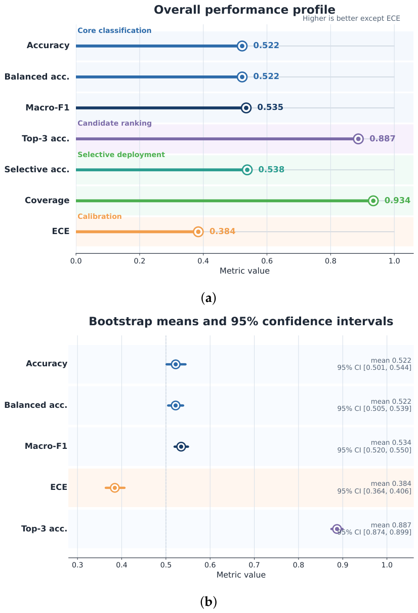
The attached performance files correspond to one fixed zero-shot evaluation of OATS-RS with a GeoRSCLIP ViT-B-32 backbone on EuroSAT RGB. Table 6 summarizes the experimental setting and Table 7 reports the main metrics. The method attains an accuracy of 0.522 and a balanced accuracy of 0.522. The equality of these two numbers is consistent with a class-balanced evaluation partition. Macro-F1 reaches 0.535, which slightly exceeds accuracy because several easy classes achieve very high precision and recall, whereas the weakest classes remain strongly under-resolved.
The most striking positive result is the top-3 accuracy of 0.887. This indicates that even when the top-ranked class is wrong, the correct label is often contained within the first few candidates. In practical remote sensing workflows, this behavior is valuable in that it suggests that the method can serve as a shortlist generator for interactive review, weak annotation, or downstream re-ranking modules. In contrast, the expected calibration error of 0.384 is high, indicating that posterior confidence is not yet reliably aligned with empirical correctness.
Bootstrap confidence intervals further show that the overall result is stable under resampling. Accuracy has a 95% interval of 0.501–0.544, balanced accuracy of 0.505–0.539, macro-F1 of 0.520–0.550, an expected calibration error of 0.364–0.406, and top-3 accuracy of 0.874–0.899. These intervals are sufficiently narrow to support the claim that the observed performance profile is not an accident of one particular test draw.
The subfigures in Figure 2a,b serve different purposes: Figure 2a summarizes the observed metric values from the final run, whereas Figure 2b visualizes bootstrap uncertainty for the metrics with available resampling intervals. Including both prevents the reader from confusing a point estimate with its sampling stability.

5.2. Ablation and Comparison Evidence Required for Full Component Attribution

Component attribution requires ablations against a GeoRSCLIP baseline and progressively enriched variants. The current supplied artifacts contain only the final full-method result, so a numerical ablation table cannot be produced without running additional experiments. Rather than inventing unsupported values, this revision adds the ablation ladder in Table 3 and the fair-comparison protocol in Table 4. These tables specify exactly which results should be added in a complete empirical resubmission: GeoRSCLIP baseline, ontology-only prompts, contrastive/confuser scoring, multi-view inference, target alignment, transductive refinement, local ambiguity experts, candidate ensembling, and selective prediction.
This distinction is important for scientific interpretation. The reported 0.522 accuracy and 0.887 top-3 accuracy characterize the complete inference stack, but do not prove that every component contributes positively. Therefore, this paper treats component attribution as an open empirical requirement rather than an established result.

5.3. Performance Is Highly Class-Dependent

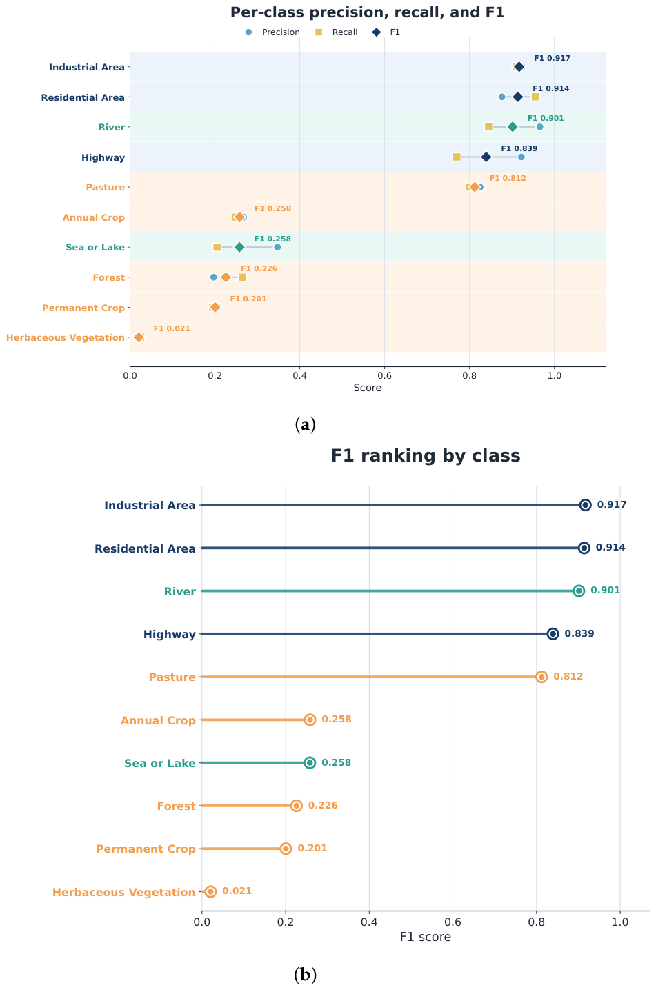
Class-wise metrics reveal a clear structural pattern: Table 8 and Figure 3 show that the model performs strongly on industrial area (F1 = 0.917), residential area (F1 = 0.914), river (F1 = 0.901), highway (F1 = 0.839), and pasture (F1 = 0.812), all of which are classes with relatively distinctive large-scale geometry, repeated texture, or strong spatial regularity. Industrial and residential scenes benefit from man-made layout priors: highways are elongated linear structures, rivers have elongated hydrographic signatures, and pasture appears easier than several neighboring vegetation categories, perhaps because it occupies a relatively consistent appearance niche in the evaluated RGB setting.
The weak end of the distribution is equally informative: the F1 scores for herbaceous vegetation, permanent crop, forest, sea or lake, and annual crop are only 0.021, 0.201, 0.226, 0.258, and 0.258, respectively. The low scores for annual crop, permanent crop, forest, and herbaceous vegetation show that the residual difficulty of the benchmark is concentrated in fine-grained vegetation semantics rather than in coarse urban–rural separation; in other words, the method is already capable of capturing scene structure when categories are strongly differentiated by geometry or layout, but remains weak when categories differ subtly in texture, canopy density, crop organization, moisture, or phenological state.
This class-dependent behavior is precisely the kind of pattern one would expect in a zero-shot remote sensing setting. Prompted text can communicate functional meaning and scene-level priors, but separability ultimately depends on whether the frozen image encoder already encodes class-discriminative cues at the right scale. For the weakest vegetation categories, the observed F1 values imply that the semantic prompt machinery is not enough to overcome the overlap in the underlying image embeddings.
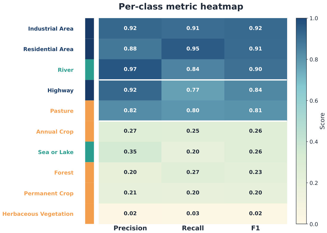
A complementary way to read the class-level evidence is to focus on metric shape rather than on a single ranking. Figure 4 shows that the hardest categories are not merely low in one of recall or precision; rather, several of them are jointly weak across all three metrics. Therefore, Figure 3 and Figure 4 are not redundant: Figure 3a compares precision, recall, and F1 side-by-side for each class, Figure 3b emphasizes the sorted F1 ranking, and Figure 4 compresses the same evidence into a dense matrix that makes class–family asymmetry easier to see. This last pattern is especially important for interpretation because it indicates a broader semantic collapse within parts of the natural-scene manifold rather than a single thresholding or calibration artifact.

5.4. Qualitative Visual Results Panel

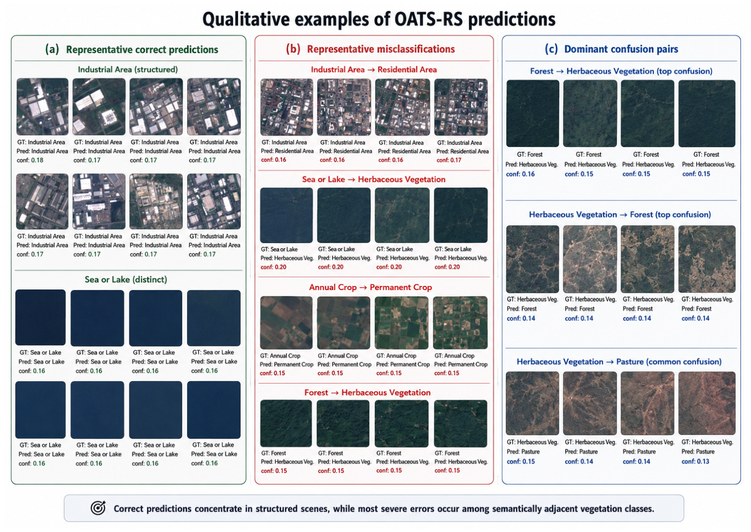
Figure 5 provides representative qualitative examples of the OATS-RS predictions. The panel complements the aggregate metrics by showing where the model performs well and where the main failure modes occur. Panel (a) shows representative correct predictions, including visually structured industrial area scenes and visually distinctive sea or lake examples. Panel (b) shows representative misclassifications, including industrial area predicted as residential area; sea or lake predicted as herbaceous vegetation; annual crop predicted as permanent crop; and forest predicted as herbaceous vegetation. Panel (c) summarizes dominant confusion pairs among visually and semantically adjacent natural classes, especially forest, herbaceous vegetation, and pasture.
These qualitative examples are not intended as additional quantitative evidence; instead, they illustrate the interpretation of the reported per-class metrics and confusion patterns. The examples show that correct predictions are concentrated in structured or visually distinctive scenes, while the most difficult cases occur among natural land cover classes with overlapping texture, color, and spatial context.

5.5. Selective Prediction Improves Reliability Only Modestly at High Coverage

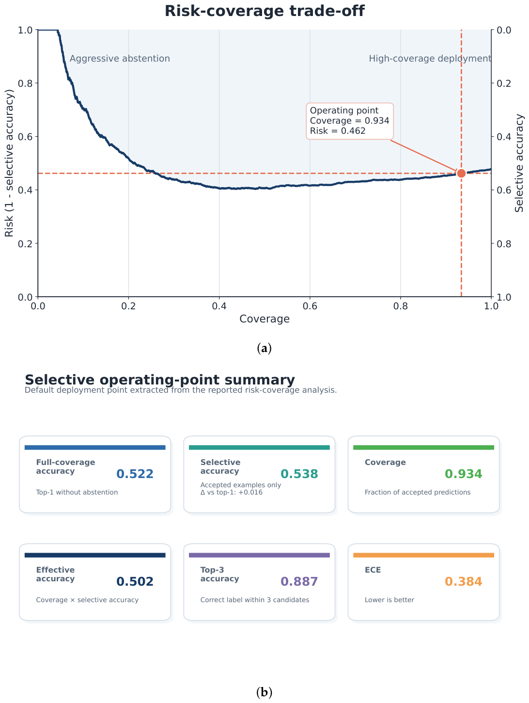
The attached result files report a default operating point with coverage of 0.934 and selective accuracy of 0.538. Because the non-selective top-1 accuracy is 0.522, the selective rule improves accepted-example accuracy by only 1.6 percentage points while abstaining on only a small fraction of the evaluation partition. The effective accuracy is 0.5025, which is simply the product of coverage and selective accuracy, and can be interpreted as the fraction of the full evaluation partition that is both accepted and correctly classified.
The risk–coverage curve and selective-summary panel in Figure 6 give a fuller picture of how abstention behaves. Table 9 summarizes representative operating points. The best selective accuracy among these points occurs around coverage 0.48–0.50, where accuracy on accepted examples rises to approximately 0.595; however, this comes at the cost of rejecting about half the test set. As coverage increases beyond 0.75, the marginal benefit of abstention declines sharply; by the default point at 0.934 coverage, the selective gain over full-coverage accuracy is small. This pattern is consistent with the elevated expected calibration error: the model can rank easy versus hard examples to some extent, but its confidence scores are not sharp enough to sustain large improvements at high coverage.
An important operational implication follows: if the application can tolerate substantial abstention, then the model can provide a reasonably accurate shortlisting mechanism for a subset of easier examples. However, if near-complete coverage is required, then selective rejection alone will not fully compensate for the underlying calibration problem. In that regime, better posterior calibration, class-specific thresholds, or explicit reject-option training may be necessary [43,47,48].

5.6. The Top-1/Top-3 Gap Indicates Unresolved but Structured Ambiguity

The difference between top-1 accuracy (0.522) and top-3 accuracy (0.887) deserves explicit discussion. In a ten-class balanced benchmark, random top-3 accuracy would be only 0.3, whereas the observed score is nearly 0.9. This implies that the model usually recognizes the relevant semantic neighborhood even when it fails to assign the highest posterior score to the correct class. Put differently, the main weakness of the proposed method is not total semantic collapse but local ranking inside a restricted set of plausible categories.
This interpretation is consistent with the per-class table. The most difficult categories are semantically and visually entangled vegetation or natural-scene classes (annual crop, permanent crop, herbaceous vegetation, forest, and to some extent sea or lake). A zero-shot model can plausibly identify such images as “natural surface” or “vegetation-related scene” while still misordering the final candidates. The strong top-3 score suggests that much of the remaining error mass is concentrated inside these local confusion neighborhoods rather than between obviously distinct classes such as residential area and river. This is encouraging for future work because local confusion is often more tractable than global confusion: it can be addressed with higher-resolution views, multispectral cues, season-aware prompting, local expert models, or class-conditional calibration.

5.7. Semantic-Family Asymmetry Is Large and Systematic

The per-class table can be compressed into a family-level view that is especially informative for remote sensing interpretation. We group the ten classes into three coarse semantic families: agriculture/vegetation (annual crop, forest, herbaceous vegetation, pasture, permanent crop), urban/transport (highway, industrial area, residential area), and hydrographic (river, sea or lake). For any group G , the mean precision, recall, and F1 are given by Equation (75) and its precision/recall analogs.
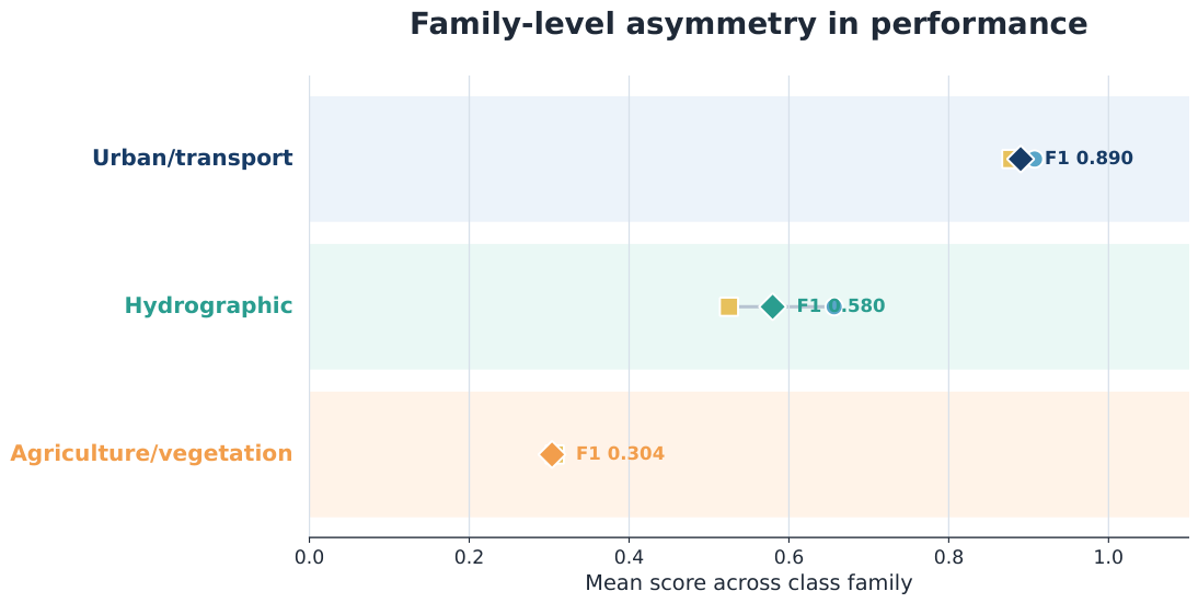
Table 10 and Figure 7 show a striking asymmetry. The urban/transport family reaches a mean F1 of 0.890, the hydrographic family 0.580, and the agriculture/vegetation family only 0.304. Therefore, the ratio between urban/transport and agriculture/vegetation mean F1 is about 2.93. This family-level disparity is more than a descriptive curiosity. It tells us that the dominant failure mode of the model is not a generic inability to read satellite scenes but a targeted weakness on the fine-grained semantics of natural surfaces.
The hydrographic family is itself internally split. For river, the F1 is 0.901, while for sea or lake it reaches only 0.258. This reveals that not all water classes are equally easy in the current zero-shot embedding geometry. Linear hydrographic structure appears to be much easier than broad water body categories for which the coastline, surrounding context, or spectral appearance may overlap with other natural classes in RGB imagery.

5.8. Annual-Crop Diagnostics Reveal a Specific Local Confusion Mode

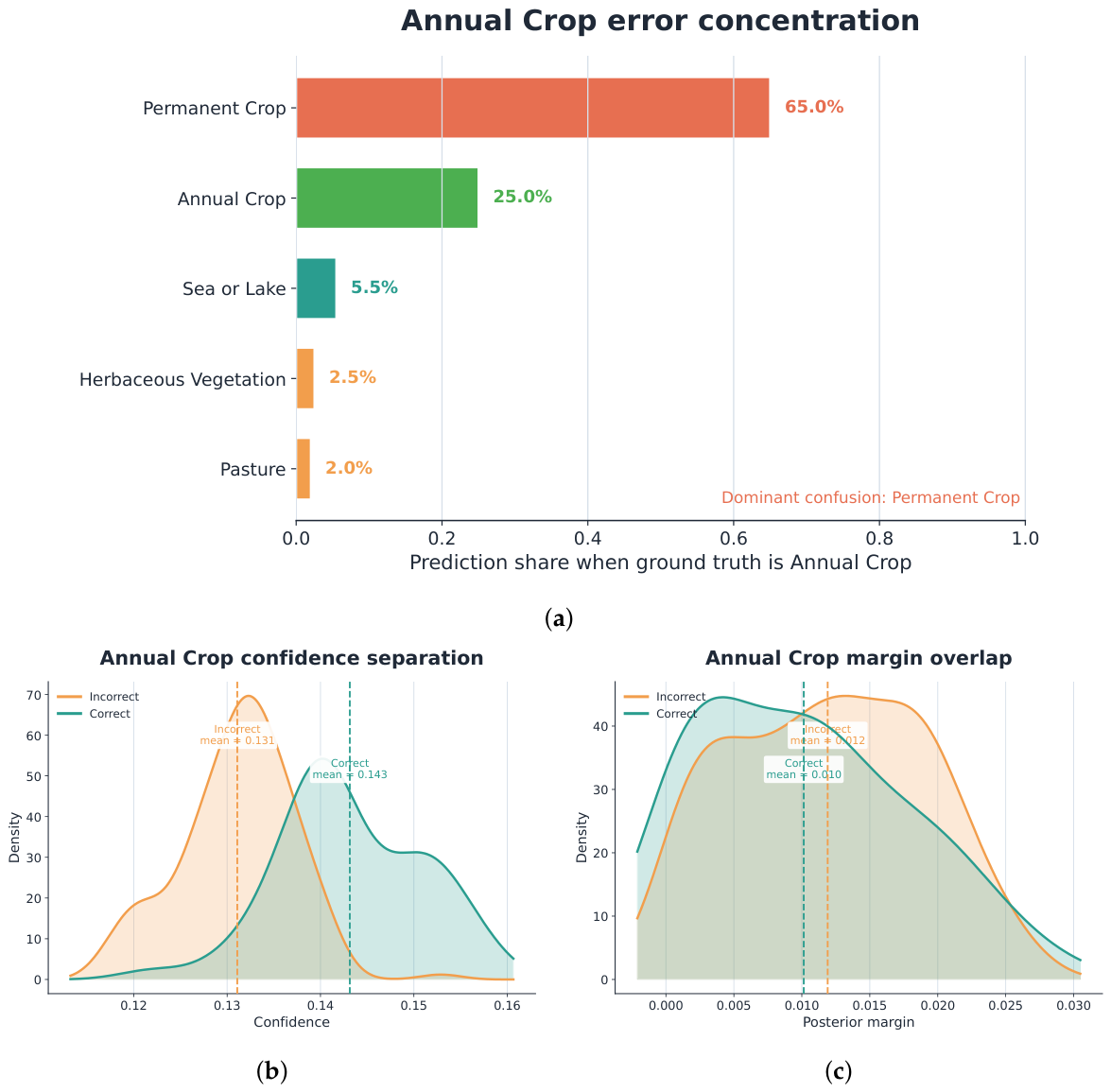
The attached prediction diagnostics file is more limited than the overall metric tables, appearing to contain only annual crop ground-truth examples. Even with that limitation, it is informative because it exposes one concrete local ambiguity neighborhood. Within this diagnostic subset, only a quarter of cases are classified correctly, matching the recall already reported in Table 8. The dominant error is confusion with permanent crop, which absorbs roughly two-thirds of the subset and consequently dominates the local failure profile. The remaining errors are distributed across sea or lake, herbaceous vegetation, and pasture at much smaller shares.
This diagnostic pattern suggests that the classifier is not merely uncertain among all natural classes; rather, it has a particularly strong bias toward ranking permanent crop above annual crop within this subset. This is exactly the kind of local ambiguity that motivates pairwise discriminative prompts and ambiguity-group re-ranking. In principle, a stronger local expert specialized to agricultural subclasses could address this specific failure mode more effectively than a global prompt bank alone.
Confidence statistics reinforce the same conclusion. The mean confidence of correct annual crop predictions in the diagnostic subset is 0.143 (standard deviation 0.008), while the mean confidence of incorrect predictions is 0.131 (standard deviation 0.006). The difference exists, but is small. Even more revealing, the mean top-1 versus top-2 margin is 0.010 for correct examples and 0.012 for incorrect examples. Thus, the raw decision margin on this subset is not a reliable discriminator of correctness. This is fully consistent with the elevated global ECE and the modest gain of selective abstention at high coverage. Table 11 summarizes these subset-level observations numerically, and Figure 8 visualizes the corresponding predicted-label distribution, confidence separation, and top-1/top-2 margin behavior.

5.9. Ranking Quality Is Stronger than Exact Top-1 Assignment

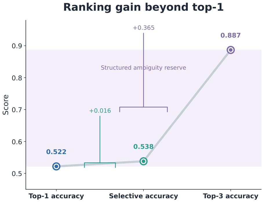
The large difference between top-1 accuracy and top-3 accuracy can be summarized visually by Figure 9. The absolute gap is
Top 3 Acc = 0.887 0.522 = 0.365 .
On a ten-class task, this is a substantial improvement over top-1 and implies that the method’s candidate ranking is materially better than its final winner-take-all decision.
This observation matters operationally. A remote sensing analyst may not always require a single decisive class label. In workflows with weak-labeling, active learning, human-in-the-loop quality control, or downstream fusion with geographic metadata, a high-quality shortlist can already be valuable. Therefore, the supplied metrics can support two complementary interpretations of OATS-RS: as a moderate zero-shot top-1 classifier, and as a substantially stronger zero-shot semantic ranker.

6. Discussion

6.1. What the Final EuroSAT Run Shows

The attached evaluation shows that OATS-RS is neither a trivial prompt-engineering baseline nor a mature universally reliable remote sensing classifier. Instead, it occupies a scientifically interesting middle ground. The model demonstrates that when equipped with ontology-aware prompting and adaptive test-time inference, a frozen remote sensing vision–language backbone can reach strong performance on several EuroSAT categories without supervised training on the target labels. The class-wise F1 values above 0.9 for industrial area, residential area, and river are difficult to dismiss; they show that zero-shot remote sensing classifiers can capture meaningful scene semantics when categories have distinctive spatial organization.
From the perspective of paper quality, this middle ground is valuable rather than embarrassing. It makes the manuscript analytically rich; the results are strong enough to justify a serious methodological treatment, but imperfect enough to expose where zero-shot remote sensing still fails. This combination supports more informative scientific discussion than a uniformly high score would. Therefore, the present evaluation contributes not merely a metric snapshot but a concrete performance geometry consisting of strong urban and linear-water recognition, weak vegetation disambiguation, sizable top-K recovery, and incomplete confidence calibration.
At the same time, the evaluation exposes precisely where the current paradigm breaks down. Herbaceous vegetation, permanent crop, forest, and annual crop remain weak, while sea or lake is markedly worse than river despite both being water-related categories. This asymmetry strongly suggests that large-scale geometric structure is captured better than subtle within-class spectral or textural variation. The result is a classifier that is excellent on some categories and fragile on others. From a deployment standpoint, this is both promising and cautionary: the model may already be useful as a pre-annotation or triage system, but is not yet a drop-in replacement for supervised remote sensing classifiers in settings dominated by fine-grained vegetation discrimination.

6.2. Why the Moderate Top-1 Accuracy Is Informative but Not Sufficient

The reported 0.522 accuracy is moderate for a classification task and should be interpreted carefully. On a balanced ten-class benchmark, random guessing produce accuracy of approximately 0.10, so 0.522 is not comparable to random guessing in a literal statistical sense; nevertheless, it is moderate relative to mature supervised remote sensing classifiers, and as such cannot support a claim of deployment-ready exact classification. Instead, its value in this manuscript is diagnostic: the result shows that the proposed method can recover strong performance on structured urban and river-like categories, while exposing severe failures in fine-grained vegetation semantics. The 0.887 top-3 accuracy further indicates that many errors are ranking errors within a plausible semantic neighborhood rather than complete semantic failures.
The calibration story is similarly mixed. Selective prediction improves accepted-example accuracy, but only modestly at high coverage. The risk–coverage curve shows that useful abstention behavior exists, yet the high expected calibration error means that probability estimates remain poorly matched to actual correctness. In practical terms, this matters because confidence values are often used for automated filtering, human workload allocation, or pseudolabel selection. A model can be semantically competent and still operationally unsafe if its confidences are miscalibrated. Therefore, the present results argue that uncertainty estimation should be treated as a first-class design objective in zero-shot remote sensing pipelines.
A key methodological insight from this study is that zero-shot classification in remote sensing benefits from being formalized as a composite inference problem rather than a single-line cosine similarity rule. The ontology-aware prompt bank helps to represent class meaning more richly than a class name alone. View-aware aggregation allows the classifier to exploit multi-scale evidence. Feature alignment and transductive refinement adapt the representation to the unlabeled target distribution. Ambiguity-group experts and selective prediction acknowledge that some decisions are intrinsically harder than others. The equations developed in this paper make these ideas explicit and modular, which should help future work to reason about which components matter most and how they interact.

6.3. Limitations Requiring Additional Experiments

Importantly, the evidence base of this manuscript is deliberately narrow. Because we only use the attached final performance files, several important claims cannot be made here. We do not report multi-dataset generalization, cross-region transfer, multispectral versus RGB comparisons, ablations against simpler prompt banks, or a direct supervised baseline trained on the same split. Thus, the manuscript is best read as a full mathematical specification and careful performance analysis of one final method instance rather than as a universal benchmark victory claim. This limitation is not a flaw in the reporting but an explicit boundary on interpretation. In particular, the component ablation table, comprehensive comparison table, AID/NWPU transfer experiments, qualitative visual examples, and measured throughput should be added once the corresponding experimental artifacts are available. Until then, this revision treats those items as required protocols and limitations, not as completed empirical claims.

6.4. Future Directions

Several future directions follow naturally from the observed performance profile. First, multispectral inputs should be studied directly, since RGB alone may not capture enough information to separate crop and vegetation subclasses; this is exactly the regime where Sentinel-2 spectral richness, SatMAE, CROMA, and other geospatial representation-learning approaches become attractive [6,8,29]. Second, time series or seasonal metadata could make class prompts far more informative for agricultural categories, echoing the importance of temporally aware land cover products such as Dynamic World [32]. Third, class-conditional calibration should replace a single global confidence threshold, in line with modern calibration work [43,44]. Fourth, ambiguity-group experts could be extended from fixed semantic groups to dynamically discovered local manifolds in the embedding space via graph-structured or propagation-based refinement [51]. Fifth, cross-taxonomy evaluation remains essential if zero-shot remote sensing classifiers are to become practical tools for label harmonization across products such as WorldCover, Dynamic World, BigEarthNet, and related archives [12,30,32,33]. Sixth, a natural extension is to couple ontology-aware scene prompting with open-vocabulary segmentation and proposal models; this would allow the same semantic machinery to not only classify geospatial concepts but to localize them [64,65,66,67].
In summary, the present results support a nuanced conclusion. Zero-shot remote sensing classification with a vision–language model adapted to remote sensing is already strong on structured classes, and often places the correct answer within a small candidate set; however, fine-grained vegetation semantics and calibrated uncertainty remain unresolved. OATS-RS provides a principled framework for addressing these issues, but the attached evaluation also makes clear that the problem is far from solved.

7. Broader Context and Forward-Looking Research Agenda

7.1. From Single-Benchmark Zero-Shot Recognition to Cross-Taxonomy Earth Observation

While the present manuscript intentionally centers one final attached EuroSAT evaluation, the larger research agenda is broader. Operational Earth observation rarely involves a single balanced ten-class benchmark. Instead, practitioners encounter shifting taxonomies, different sensor stacks, and different spatial scales across products such as Dynamic World, WorldCover, BigEarthNet, BigEarthNet-MM, LoveDA, and GEO-Bench [12,30,31,32,33,36]. A compelling next step is cross-taxonomy evaluation, where the ontology-aware prompt machinery is asked not merely to classify within one fixed label set but to mediate between heterogeneous label systems. This is also where newer geospatial foundation models such as RingMo, SatlasPretrain, MMEarth, DOFA, AnySat, and Prithvi-EO become especially relevant [37,38,39,40,41,42].

7.2. Trustworthy Deployment, Abstention, and Analyst Workflows

A second priority is trustworthy deployment. In practical remote sensing operations, a classifier is often embedded inside a longer decision pipeline that includes human review, geospatial context, temporal change analysis, and often explicit abstention rules. For this reason, calibration, reject-option learning, set-valued prediction, and conformal wrappers are not peripheral topics but central deployment tools [43,44,61,62,63]. The attached final run already hints at this need: top-3 performance is strong, but confidence calibration is weak. This combination argues for a workflow in which zero-shot remote sensing systems surface semantically plausible candidates, expose uncertainty, and abstain when necessary rather than forcing every image into a single overconfident label. Classical approaches such as Platt scaling, modern verified calibration methods, Bayesian approximations, and test-time adaptation should all be viewed as complementary rather than competing tools in this pipeline [52,53,54,55,56,57,58,59,60].

7.3. Towards Open-Vocabulary and Multimodal Earth Vision Systems

A third direction is to connect zero-shot scene classification with open-vocabulary dense prediction and richer multimodal reasoning. Open-vocabulary remote sensing segmentation, training-free segmentation, and SAM-guided earth vision systems show that language supervision can be used at more granular levels than image-wise scene labels [64,65,66,67]. Meanwhile, multimodal geospatial foundation models are beginning to unify optical, SAR, temporal, and other modalities under one pretraining umbrella [8,40,41,42]. The ontology-aware design advocated for in this paper is compatible with this trajectory: once class semantics are represented explicitly, they can in principle condition classification, segmentation, retrieval, or even interactive geospatial analysis. This suggests that the value of the present method may extend beyond the single benchmark studied here, even though only the attached EuroSAT performance files are analyzed empirically in this manuscript.

7.4. Reproducibility, Benchmarking, and Inferential Restraint

Finally, the literature on geospatial foundation models is becoming increasingly aware that large-scale evaluation must be matched by careful inferential restraint. Surveys, benchmark papers, and meta-analyses repeatedly emphasize how strongly conclusions can depend on modality, resolution, split definition, region, and task formulation [9,10,11,17,18,19,20,36]. The present manuscript follows this principle by restricting all empirical claims to the attached final result files. This restriction narrows the scope of the claims, but also makes the argument cleaner: the paper presents a rich method, a mathematically explicit inference formulation, and a careful analysis of one final observed performance profile, without pretending to demonstrate universality where the evidence is not yet available.

8. Conclusions

This paper presents OATS-RS as a deliberately inference-centric framework for zero-shot remote sensing scene classification. Rather than relying on a single text prompt and single image crop, the proposed method combines ontology-aware prompt construction, confuser-aware scoring, hierarchical gating, adaptive multi-view aggregation, target-space feature alignment, balanced transductive refinement, local ambiguity experts, and selective prediction. The mathematical treatment shows that these components can be interpreted coherently as margin-shaping, distribution-matching, and uncertainty-aware inference operations carried out on top of a frozen remote sensing-adapted vision–language backbone.
The empirical evidence used in the manuscript is intentionally narrow: one final GeoRSCLIP ViT-B-32 evaluation on EuroSAT RGB using a balanced held-out partition. Within this scope, the method reaches 0.522 accuracy, 0.535 macro-F1, and 0.887 top-3 accuracy. The strongest classes are industrial area, residential area, river, highway, and pasture, while the weakest are herbaceous vegetation, permanent crop, forest, annual crop, and sea or lake. Selective rejection increases accepted-example accuracy only modestly at high coverage, and calibration remains imperfect. These observations suggest that the central open challenge is no longer coarse scene recognition but fine-grained semantic ranking and calibrated uncertainty among closely related natural classes.
The broader value of the manuscript lies in its explicit decomposition of zero-shot remote sensing inference. By turning the pipeline into a structured mathematical object, this paper provides a foundation for future work that may incorporate multispectral evidence, temporal context, stronger local experts, or more principled calibration while keeping the same high-level zero-shot philosophy.

Funding

This research received no external funding.

Data Availability Statement

The quantitative results analyzed in this manuscript are derived from image-level evaluation records along with the attached performance files accompanying the submission, including the overall metric summary, bootstrap confidence intervals, per-class precision/recall/F1 table, and risk–coverage curve. The reported accuracy, precision, recall, F1, top-K accuracy, calibration, and selective-prediction statistics require ground-truth labels, predicted labels, scores, and accept/abstain decisions at the image level. The underlying benchmark is EuroSAT [9]. The manuscript source and generated figures are provided with this submission package. A curated qualitative montage of selected satellite thumbnails is not included in the present package.

Acknowledgments

The author thanks the maintainers of open remote sensing datasets and remote sensing vision–language models that make reproducible zero-shot evaluation possible.

Conflicts of Interest

Author János Horváth was employed by the company Visionary Tech Event Solutions. The author declares that the research was conducted in the absence of any commercial or financial relationships that could be construed as a potential conflict of interest.

Appendix A. Notation and Symbol Table

Table A1 collects the most important symbols used in the manuscript. The notation is intentionally redundant with the main text so that the appendix can serve as a compact reference during reading.
Table A1. Core notation used throughout the manuscript.
SymbolMeaning
C Set of scene classes. In the reported benchmark, | C | = 10 .
x X Input RGB remote sensing image patch.
y C Ground-truth class label.
f θ Frozen image encoder of the remote sensing vision–language model.
g ϕ Frozen text encoder of the remote-sensing vision–language model.
z ( x ) l 2 -normalized image embedding of x.
t ( p ) l 2 -normalized text embedding of prompt p.
P c + Positive prompt family for class c.
P c Negative or confuser prompt family for class c.
G Set of prompt groups such as literal, scene, context, geometry, signature, and pairwise groups.
u c + Aggregated positive text prototype for class c.
u c Aggregated confuser prototype for class c.
λ neg Weight of the confuser penalty.
Δ c , d ( x ) Pairwise discriminative margin between classes c and d.
λ rel Weight of pairwise relational corrections.
λ h Weight of hierarchical parent gating.
V ( x ) Set of test-time views associated with image x.
ω m ( x ) Adaptive weight of view m for image x.
z ¯ ( x ) Aggregated multi-view image embedding.
A Target-distribution alignment operator derived from unlabeled target covariance.
z al ( x ) Aligned image embedding after feature adaptation.
q i c Soft assignment of target image i to class c during transductive refinement.
μ c Refined class prototype for class c.
b Vector of class bias terms enforcing the target prior.
π c ( x ) Final class posterior assigned to class c.
κ ( x ) Maximum posterior confidence used for selective prediction.
τ Confidence threshold for the selective classifier.
Cov ( τ ) Coverage of the selective classifier.
Acc sel ( τ ) Accuracy on accepted examples at threshold τ .
Acc eff ( τ ) Effective accuracy equal to coverage times selective accuracy.
Top K Top-K accuracy.
R K Ambiguity recovery ratio derived from top-K accuracy.
F 1 ¯ ( G l ) Mean class-wise F1 across a semantic family G l .
D Semantic disparity index over family-level F1 scores.

Appendix B. Additional Derivations

Appendix B.1. Softmax Posterior and Temperature-Scaled Logits

Let l c ( x ) denote the final class logit after all image-side and text-side adjustments. The posterior used for classification is
π c ( x ) = exp ( l c ( x ) / τ π ) r = 1 C exp ( l r ( x ) / τ π ) ,
where τ π > 0 is an optional temperature. If τ π = 1 , the logits are left unchanged; if τ π > 1 , the predictive distribution is softened; and if τ π < 1 , it is sharpened. The derivative of the posterior with respect to the logit of class d is
π c ( x ) l d ( x ) = 1 τ π π c ( x ) 1 { c = d } π d ( x ) .
Equation (A2) is useful for understanding why overconfident logits can dominate the selective prediction behavior, because confidence is a highly nonlinear function of relative rather than absolute score differences.

Appendix B.2. Derivation of the Prototype Update

Consider the prototype subproblem
max μ c 2 = 1 i = 1 n q i c γ z i μ c + λ μ u c + μ c .
Introducing a Lagrange multiplier λ c for the norm constraint gives
L ( μ c , λ c ) = i = 1 n q i c γ z i μ c + λ μ u c + μ c λ c ( μ c μ c 1 ) .
Differentiating with respect to μ c yields
i = 1 n q i c γ z i + λ μ u c + = 2 λ c μ c .
Hence, the maximizer is proportional to the vector sum on the left-hand side, leading directly to Equation (65) after normalization.

Appendix B.3. Selective Prediction and Effective Accuracy

The selective classifier accepts image x i when κ ( x i ) τ . Let a i ( τ ) = 1 { κ ( x i ) τ } denote the acceptance indicator. Coverage and selective accuracy can then be written more compactly as
Cov ( τ ) = 1 n i = 1 n a i ( τ ) ,
Acc sel ( τ ) = i = 1 n a i ( τ ) 1 { y ^ ( x i ) = y i } i = 1 n a i ( τ ) .
Multiplying the two equations yields
Acc eff ( τ ) = 1 n i = 1 n a i ( τ ) 1 { y ^ ( x i ) = y i } ,
showing that effective accuracy is exactly the fraction of the original test set that is both accepted and correctly classified.

Appendix B.4. Macro-F1 and Balanced Accuracy

Balanced accuracy and macro-F1 are related but distinct. Balanced accuracy averages only recalls:
BAcc = 1 C c = 1 C R c .
Macro-F1 instead averages the harmonic mean of precision and recall per-class:
MacroF 1 = 1 C c = 1 C 2 P c R c P c + R c .
In a balanced benchmark, the difference between the two metrics reveals whether precision is systematically better or worse than recall across classes. In the attached EuroSAT evaluation, macro-F1 (0.535) is slightly above balanced accuracy (0.522), suggesting that high-precision easy classes partially offset the recall weaknesses of the hardest categories.

Appendix B.5. Expected Calibration Error

Suppose that confidence values are partitioned into B bins. For bin b, define the empirical accuracy and average confidence
acc ( B b ) = 1 | B b | i B b 1 { y ^ ( x i ) = y i } , conf ( B b ) = 1 | B b | i B b κ ( x i ) .
Then, the ECE is
ECE = b = 1 B | B b | n acc ( B b ) conf ( B b ) .
A large ECE can arise from either overconfidence or underconfidence, and does not identify the direction of miscalibration on its own. The attached files report only the scalar ECE summary; thus, the present manuscript treats it as a global warning flag rather than as a fully-resolved calibration diagnosis.

Appendix B.6. Top-K Monotonicity and Shortlist Utility

The shortlist utility in Equation (47) immediately yields a monotonicity property. If 1 K 1 < K 2 C , then
A K 1 ( x ) A K 2 ( x )
for every image x; therefore,
u K 1 ( x , y ) u K 2 ( x , y ) .
Averaging over the test set gives
U K 1 U K 2 .
The practical interpretation is that top-K metrics quantify the extent to which the classifier has localized the correct semantic neighborhood, even when exact rank-1 assignment remains unstable.

Appendix B.7. Bootstrap Percentile Intervals

Suppose that a scalar metric m ( D ) is estimated on a dataset D = { ( x i , y i ) } i = 1 n . In nonparametric bootstrap resampling [69], B resampled datasets D ( 1 ) , , D ( B ) are formed by sampling with replacement from D . The bootstrap mean is
m ¯ boot = 1 B b = 1 B m ( D ( b ) )
and the percentile interval at confidence level 1 α is
I 1 α ( m ) = Q α / 2 { m ( D ( b ) ) } b = 1 B , Q 1 α / 2 { m ( D ( b ) ) } b = 1 B ,
where Q q ( · ) denotes the empirical q-quantile. The attached result files provide such intervals for accuracy, balanced accuracy, macro-F1, ECE, and top-3 accuracy.

Appendix B.8. Family-Conditioned Disparity Indices

Given the family averages F 1 ¯ f from Equation (48), it is possible to define several summary indices. The absolute family gap is Equation (49). A scale-normalized alternative is
ρ F = max f F F 1 ¯ f min f F F 1 ¯ f + ε ,
with a small ε > 0 for numerical stability. Another useful quantity is the family variance,
V F = 1 | F | f F F 1 ¯ f 1 | F | g F F 1 ¯ g 2 .
Large D F , ρ F , or V F indicate that model quality is concentrated in some semantic regions of the taxonomy and weak in others.

Appendix B.9. Set-Valued Prediction and Abstention Utility

Selective prediction can also be written as a utility maximization problem. Let C ( τ ) = Cov ( τ ) and R ( τ ) = 1 Acc sel ( τ ) denote coverage and selective risk. A simple utility functional is
U ( τ ; λ ) = C ( τ ) 1 R ( τ ) λ 1 C ( τ ) ,
where λ 0 is the opportunity cost of abstention. If a system instead outputs a set of labels of variable size, it is possible to use
U set ( τ , γ ) = 1 n i = 1 n 1 { y i S τ ( x i ) } γ | S τ ( x i ) | ,
where S τ ( x i ) is a thresholded candidate set and γ penalizes ambiguity. This naturally connects zero-shot remote sensing classification to the literature on set-valued prediction and reject-option learning [61,62,63].

Appendix C. Extended Result Tables

Table A2 reproduces the supplied bootstrap intervals in compact form, while Table A3 collects a few quantities derived directly from the attached primary metrics.
Table A2. Bootstrap summary reproduced from the attached result file.
MetricMeanStd. Dev.95% CI Low95% CI High
Accuracy0.52210.01060.50150.5443
Balanced accuracy0.52190.00850.50500.5389
Macro-F10.53440.00780.51960.5500
Expected calibration error0.38430.01060.36390.4063
Top-3 accuracy0.88700.00650.87420.8995
Table A3. Derived quantities computed from the attached final metrics.
Derived QuantityFormulaValue
Top-3 gap Top 3 Acc 0.365
Ambiguity-recovery ratio ( Top 3 Acc ) / ( 1 Acc ) 0.764
Selective gain at reported threshold Acc sel Acc 0.016
Urban/agriculture F1 ratio F 1 ¯ urban / F 1 ¯ agri 2.932
Hydro/agriculture F1 ratio F 1 ¯ hydro / F 1 ¯ agri 1.909

Appendix D. Algorithmic Summary

For completeness, Table A4 summarizes the overall pipeline in compact textual form.
Table A4. Algorithmic summary of OATS-RS.
StepOperation
1For each class, construct ontology-aware prompt families including literal prompts, scene descriptions, contextual prompts, signature prompts, and pairwise contrastive prompts.
2Encode all prompts with the frozen text encoder and aggregate them into positive and negative class prototypes.
3For each image, generate multiple test-time views, encode them with the frozen image encoder, and compute adaptive view weights from confidence, margin, entropy, and agreement.
4Aggregate the view embeddings into a single image representation and apply target-distribution feature alignment.
5Compute base class scores from positive similarity minus confuser penalty, then add pairwise relational and hierarchical corrections.
6Perform balanced transductive refinement on the unlabeled target set by iterating soft assignments, prototype updates, and class-bias corrections.
7Apply local ambiguity-group experts, graph smoothing, density re-ranking, and candidate-ensemble fusion where available.
8Produce final class posteriors, top-K rankings, and the selective decision rule obtained by thresholding confidence.
9Evaluate accuracy, balanced accuracy, macro-F1, calibration, top-K performance, and risk–coverage behavior on the labeled test set.

References

  1. Dosovitskiy, A.; Beyer, L.; Kolesnikov, A.; Weissenborn, D.; Zhai, X.; Unterthiner, T.; Dehghani, M.; Minderer, M.; Heigold, G.; Gelly, S.; et al. An Image is Worth 16x16 Words: Transformers for Image Recognition at Scale. In Proceedings of the International Conference on Learning Representations, Virtual, 3–7 May 2021. [Google Scholar]
  2. Radford, A.; Kim, J.W.; Hallacy, C.; Ramesh, A.; Goh, G.; Agarwal, S.; Sastry, G.; Askell, A.; Mishkin, P.; Clark, J.; et al. Learning Transferable Visual Models From Natural Language Supervision. arXiv 2021, arXiv:2103.00020. [Google Scholar] [CrossRef] [Scilit]
  3. Zhai, X.; Wang, X.; Mustafa, B.; Steiner, A.; Keysers, D.; Kolesnikov, A.; Beyer, L. LiT: Zero-Shot Transfer With Locked-Image Text Tuning. In Proceedings of the IEEE/CVF Conference on Computer Vision and Pattern Recognition, New Orleans, LA, USA, 18–24 June 2022; pp. 18123–18133. [Google Scholar] [CrossRef] [Scilit]
  4. Cherti, M.; Beaumont, R.; Wightman, R.; Wortsman, M.; Ilharco, G.; Gordon, C.; Schuhmann, C.; Schmidt, L.; Jitsev, J. Reproducible Scaling Laws for Contrastive Language-Image Learning. In Proceedings of the IEEE/CVF Conference on Computer Vision and Pattern Recognition, Vancouver, BC, Canada, 17–24 June 2023; pp. 2818–2829. [Google Scholar] [CrossRef] [Scilit]
  5. Oquab, M.; Darcet, T.; Moutakanni, T.; Vo, H.; Szafraniec, M.; Khalidov, V.; Fernandez, P.; Haziza, D.; Massa, F.; El-Nouby, A.; et al. DINOv2: Learning Robust Visual Features without Supervision. arXiv 2023, arXiv:2304.07193. [Google Scholar] [CrossRef] [Scilit]
  6. Cong, Y.; Khanna, S.; Meng, C.; Liu, P.; Rozi, E.; He, Y.; Burke, M.; Lobell, D.; Ermon, S. SatMAE: Pre-training Transformers for Temporal and Multi-Spectral Satellite Imagery. Adv. Neural Inf. Process. Syst. 2022, 35, 197–211. [Google Scholar] [CrossRef] [Scilit]
  7. Gupta, R.; Reed, C.; Li, S.; Brockman, S.; Funk, C.; Clipp, B.; Keutzer, K.; Candido, S.; Uyttendaele, M.; Darrell, T. Scale-MAE: A Scale-Aware Masked Autoencoder for Multiscale Geospatial Representation Learning. In Proceedings of the IEEE/CVF International Conference on Computer Vision, Paris, France, 1–6 October 2023. [Google Scholar] [CrossRef] [Scilit]
  8. Fuller, A.; Millard, K.; Green, J.R. CROMA: Remote Sensing Representations with Contrastive Radar-Optical Masked Autoencoders. Adv. Neural Inf. Process. Syst. 2023, 36, 5506–5538. [Google Scholar] [CrossRef] [Scilit]
  9. Helber, P.; Bischke, B.; Dengel, A.; Borth, D. EuroSAT: A Novel Dataset and Deep Learning Benchmark for Land Use and Land Cover Classification. IEEE J. Sel. Top. Appl. Earth Obs. Remote Sens. 2019, 12, 2217–2226. [Google Scholar] [CrossRef] [Scilit]
  10. Xia, G.S.; Hu, J.; Hu, F.; Shi, B.; Bai, X.; Zhong, Y.; Zhang, L.; Lu, X. AID: A Benchmark Data Set for Performance Evaluation of Aerial Scene Classification. IEEE Trans. Geosci. Remote Sens. 2017, 55, 3965–3981. [Google Scholar] [CrossRef] [Scilit]
  11. Cheng, G.; Han, J.; Lu, X. Remote Sensing Image Scene Classification: Benchmark and State of the Art. Proc. IEEE 2017, 105, 1865–1883. [Google Scholar] [CrossRef] [Scilit]
  12. Sumbul, G.; Charfuelan, M.; Demir, B.; Markl, V. BigEarthNet: A Large-Scale Benchmark Archive for Remote Sensing Image Understanding. In Proceedings of the IEEE International Geoscience and Remote Sensing Symposium (IGARSS), Yokohama, Japan, 28 July–2 August 2019; pp. 5901–5904. [Google Scholar] [CrossRef] [Scilit]
  13. Schmitt, M.; Hughes, L.H.; Qiu, C.; Zhu, X.X. SEN12MS – A Curated Dataset of Georeferenced Multi-Spectral Sentinel-1/2 Imagery for Deep Learning and Data Fusion. Isprs Ann. Photogramm. Remote Sens. Spat. Inf. Sci. 2019, IV-2/W7, 153–160. [Google Scholar] [CrossRef] [Scilit]
  14. Zhou, K.; Yang, J.; Loy, C.C.; Liu, Z. Learning to Prompt for Vision-Language Models. Int. J. Comput. Vis. 2022, 130, 2337–2348. [Google Scholar] [CrossRef] [Scilit]
  15. Zhou, K.; Yang, J.; Loy, C.C.; Liu, Z. Conditional Prompt Learning for Vision-Language Models. In Proceedings of the IEEE/CVF Conference on Computer Vision and Pattern Recognition, New Orleans, LA, USA, 18–24 June 2022; pp. 16816–16825. [Google Scholar] [CrossRef] [Scilit]
  16. Khattak, M.U.; Rasheed, H.; Maaz, M.; Khan, S.; Khan, F.S. MaPLe: Multi-Modal Prompt Learning. In Proceedings of the IEEE/CVF Conference on Computer Vision and Pattern Recognition, Vancouver, BC, Canada, 17–24 June 2023; pp. 19113–19122. [Google Scholar] [CrossRef] [Scilit]
  17. Gu, Y.; Wang, Y.; Li, Y. A Survey on Deep Learning-Driven Remote Sensing Image Scene Understanding: Scene Classification, Scene Retrieval and Scene-Guided Object Detection. Appl. Sci. 2019, 9, 2110. [Google Scholar] [CrossRef] [Scilit]
  18. Thapa, A.; Horanont, T.; Neupane, B.; Aryal, J. Deep Learning for Remote Sensing Image Scene Classification: A Review and Meta-Analysis. Remote Sens. 2023, 15, 4804. [Google Scholar] [CrossRef] [Scilit]
  19. Zhou, W.; Newsam, S.; Li, C.; Shao, Z. PatternNet: A Benchmark Dataset for Performance Evaluation of Remote Sensing Image Retrieval. ISPRS J. Photogramm. Remote Sens. 2018, 145, 197–209. [Google Scholar] [CrossRef] [Scilit]
  20. Zhu, X.X.; Hu, J.; Qiu, C.; Shi, Y.; Kang, J.; Mou, L.; Bagheri, H.; Häberle, M.; Hua, Y.; Huang, R.; et al. So2Sat LCZ42: A Benchmark Dataset for Global Local Climate Zones Classification. arXiv 2019, arXiv:1912.12171. [Google Scholar] [CrossRef] [Scilit]
  21. Jia, C.; Yang, Y.; Xia, Y.; Chen, Y.; Parekh, Z.; Pham, H.; Le, Q.V.; Sung, Y.; Li, Z.; Duerig, T. Scaling Up Visual and Vision-Language Representation Learning With Noisy Text Supervision. In Proceedings of the 38th International Conference on Machine Learning, Virtual, 18–24 July 2021; Volume 139, pp. 4904–4916. [Google Scholar]
  22. Khattak, M.U.; Wasim, S.T.; Naseer, M.; Khan, S.; Yang, M.H.; Khan, F.S. Self-Regulating Prompts: Foundational Model Adaptation without Forgetting. In Proceedings of the IEEE/CVF International Conference on Computer Vision, Paris, France, 1–6 October 2023; pp. 15190–15200. [Google Scholar]
  23. Zhang, R.; Zhang, W.; Fang, R.; Gao, P.; Li, K.; Dai, J.; Qiao, Y.; Li, H. Tip-Adapter: Training-Free Adaption of CLIP for Few-Shot Classification. In Proceedings of the European Conference on Computer Vision, Tel Aviv, Israel, 23–27 October 2022; pp. 493–510. [Google Scholar]
  24. Shu, M.; Nie, W.; Huang, D.A.; Yu, Z.; Goldstein, T.; Anandkumar, A.; Xiao, C. Test-Time Prompt Tuning for Zero-Shot Generalization in Vision-Language Models. In Proceedings of the Advances in Neural Information Processing Systems, New Orleans, LA, USA, 28 November–9 December 2022; Volume 35. [Google Scholar] [CrossRef] [Scilit]
  25. Gao, P.; Geng, S.; Zhang, R.; Ma, T.; Fang, R.; Zhang, Y.; Li, H.; Qiao, Y. CLIP-Adapter: Better Vision-Language Models with Feature Adapters. arXiv 2021, arXiv:2110.04544. [Google Scholar] [CrossRef] [Scilit]
  26. Jia, M.; Tang, L.; Chen, B.C.; Cardie, C.; Belongie, S.; Hariharan, B.; Lim, S.N. Visual Prompt Tuning. In Proceedings of the European Conference on Computer Vision, Tel Aviv, Israel, 23–27 October 2022; pp. 709–727. [Google Scholar] [CrossRef] [Scilit]
  27. Schuhmann, C.; Beaumont, R.; Vencu, R.; Gordon, C.; Wightman, R.; Cherti, M.; Coombes, T.; Katta, A.; Mullis, C.; Wortsman, M.; et al. LAION-5B: An Open Large-Scale Dataset for Training Next Generation Image-Text Models. Adv. Neural Inf. Process. Syst. 2022, 35, 25278–25294. [Google Scholar] [CrossRef] [Scilit]
  28. Zhai, X.; Mustafa, B.; Kolesnikov, A.; Beyer, L. Sigmoid Loss for Language Image Pre-Training. arXiv 2023, arXiv:2303.15343. [Google Scholar] [CrossRef] [Scilit]
  29. Drusch, M.; Del Bello, U.; Carlier, S.; Colin, O.; Fernandez, V.; Gascon, F.; Hoersch, B.; Isola, C.; Laberinti, P.; Martimort, P.; et al. Sentinel-2: ESA’s Optical High-Resolution Mission for GMES Operational Services. Remote Sens. Environ. 2012, 120, 25–36. [Google Scholar] [CrossRef] [Scilit]
  30. Sumbul, G.; de Wall, A.; Kreuziger, T.; Marcelino, F.; Costa, H.; Benevides, P.; Caetano, M.; Demir, B.; Markl, V. BigEarthNet-MM: A Large Scale Multi-Modal Multi-Label Benchmark Archive for Remote Sensing Image Classification and Retrieval. arXiv 2021, arXiv:2105.07921. [Google Scholar] [CrossRef] [Scilit]
  31. Wang, J.; Zheng, Z.; Ma, A.; Lu, X.; Zhong, Y. LoveDA: A Remote Sensing Land-Cover Dataset for Domain Adaptive Semantic Segmentation. arXiv 2021, arXiv:2110.08733. [Google Scholar] [CrossRef] [Scilit]
  32. Brown, C.F.; Brumby, S.P.; Guzder-Williams, B.; Birch, T.; Hyde, S.B.; Mazzariello, J.; Czerwinski, W.; Pasquarella, V.J.; Haertel, R.; Ilyushchenko, S.; et al. Dynamic World, Near Real-Time Global 10 m Land Use Land Cover Mapping. Sci. Data 2022, 9, 251. [Google Scholar] [CrossRef] [Scilit]
  33. Zanaga, D.; Van De Kerchove, R.; Daems, D.; De Keersmaecker, W.; Brockmann, C.; Kirches, G.; Wevers, J.; Cartus, O.; Santoro, M.; Fritz, S.; et al. ESA WorldCover 10 m 2021 v200. Dataset Release. 2022. Available online: https://zenodo.org/records/7254221 (accessed on 28 May 2026).
  34. Liu, F.; Chen, D.; Guan, Z.; Zhou, X.; Zhu, J.; Ye, Q.; Fu, L.; Zhou, J. RemoteCLIP: A Vision Language Foundation Model for Remote Sensing. IEEE Trans. Geosci. Remote Sens. 2024, 62, 5622216. [Google Scholar] [CrossRef] [Scilit]
  35. Zhang, Z.; Zhao, T.; Guo, Y.; Yin, J. RS5M and GeoRSCLIP: A Large-Scale Vision-Language Dataset and a Large Vision-Language Model for Remote Sensing. IEEE Trans. Geosci. Remote Sens. 2024, 62, 5642123. [Google Scholar] [CrossRef] [Scilit]
  36. Lacoste, A.; Lehmann, N.; Rodriguez, O.; Sherwin, E.; Kerner, H.; Lutjens, B.; Zhu, X. GEO-Bench: Toward Foundation Models for Earth Monitoring. arXiv 2023, arXiv:2306.03831. [Google Scholar] [CrossRef] [Scilit]
  37. Sun, X.; Wang, P.; Lu, W.; Zhu, Z.; Lu, X.; He, Q.; Li, J.; Rong, X.; Yang, Z.; Chang, H.; et al. RingMo: A Remote Sensing Foundation Model with Masked Image Modeling. IEEE Trans. Geosci. Remote Sens. 2023, 61, 5612822. [Google Scholar] [CrossRef] [Scilit]
  38. Bastani, F.; Wolters, P.; Gupta, R.; Ferdinando, J.; Kembhavi, A. SatlasPretrain: A Large-Scale Dataset for Remote Sensing Image Understanding. In Proceedings of the IEEE/CVF International Conference on Computer Vision, Paris, France, 1–6 October 2023; pp. 16772–16782. [Google Scholar]
  39. Nedungadi, V.; Kariryaa, A.; Oehmcke, S.; Belongie, S.; Igel, C.; Lang, N. MMEarth: Exploring Multi-Modal Pretext Tasks for Geospatial Representation Learning. In Proceedings of the European Conference on Computer Vision, Milan, Italy, 29 September–4 October 2024. [Google Scholar]
  40. Xiong, Z.; Wang, Y.; Zhang, F.; Stewart, A.J.; Hanna, J.; Borth, D.; Papoutsis, I.; Le Saux, B.; Camps-Valls, G.; Zhu, X.X. Neural Plasticity-Inspired Multimodal Foundation Model for Earth Observation. arXiv 2024, arXiv:2403.15356. [Google Scholar] [CrossRef] [Scilit]
  41. Astruc, G.; Gonthier, N.; Mallet, C.; Landrieu, L. AnySat: An Earth Observation Model for Any Resolutions, Scales, and Modalities. arXiv 2024, arXiv:2412.14123. [Google Scholar] [CrossRef] [Scilit]
  42. Szwarcman, D.; Roy, S.; Fraccaro, P.; Gislason, O.E.; Blumenstiel, B.; Ghosal, R.; Moreno, J.B. Prithvi-EO-2.0: A Versatile Multi-Temporal Foundation Model for Earth Observation Applications. arXiv 2024, arXiv:2412.02732. [Google Scholar] [CrossRef] [Scilit]
  43. Guo, C.; Pleiss, G.; Sun, Y.; Weinberger, K.Q. On Calibration of Modern Neural Networks. In Proceedings of the 34th International Conference on Machine Learning, Sydney, Australia, 6–11 August 2017; Volume 70, pp. 1321–1330. [Google Scholar]
  44. Minderer, M.; Djolonga, J.; Romijnders, R.; Hubis, F.; Zhai, X.; Houlsby, N.; Tran, D.; Lucic, M. Revisiting the Calibration of Modern Neural Networks. In Proceedings of the Advances in Neural Information Processing Systems, Online, 6–14 December 2021; Volume 34. [Google Scholar]
  45. Lakshminarayanan, B.; Pritzel, A.; Blundell, C. Simple and Scalable Predictive Uncertainty Estimation Using Deep Ensembles. In Proceedings of the Advances in Neural Information Processing Systems, Long Beach, CA, USA, 4–9 December 2017; Volume 30. [Google Scholar]
  46. Hendrycks, D.; Gimpel, K. A Baseline for Detecting Misclassified and Out-of-Distribution Examples in Neural Networks. In Proceedings of the International Conference on Learning Representations, Toulon, France, 24–26 April 2017. [Google Scholar]
  47. Geifman, Y.; El-Yaniv, R. Selective Classification for Deep Neural Networks. In Proceedings of the Advances in Neural Information Processing Systems, Long Beach, CA, USA, 4–9 December 2017; Volume 30. [Google Scholar]
  48. Geifman, Y.; El-Yaniv, R. SelectiveNet: A Deep Neural Network with an Integrated Reject Option. In Proceedings of the 36th International Conference on Machine Learning, Long Beach, CA, USA, 9-15 June 2019; Volume 97, pp. 2151–2159. [Google Scholar]
  49. Dempster, A.P.; Laird, N.M.; Rubin, D.B. Maximum Likelihood from Incomplete Data via the EM Algorithm. J. R. Stat. Soc. Ser. B 1977, 39, 1–38. [Google Scholar] [CrossRef] [Scilit]
  50. Grandvalet, Y.; Bengio, Y. Semi-Supervised Learning by Entropy Minimization. In Proceedings of the Advances in Neural Information Processing Systems, Vancouver, Canada, 13–18 December 2004; Volume 17. [Google Scholar]
  51. Zhou, D.; Bousquet, O.; Lal, T.N.; Weston, J.; Scholkopf, B. Learning with Local and Global Consistency. In Proceedings of the Advances in Neural Information Processing Systems, Vancouver, Canada, 13–18 December 2004; Volume 16, pp. 321–328. [Google Scholar]
  52. Wang, D.; Shelhamer, E.; Liu, S.; Olshausen, B.; Darrell, T. Tent: Fully Test-Time Adaptation by Entropy Minimization. In Proceedings of the International Conference on Learning Representations, Virtual Event, 3–7 May 2021. [Google Scholar]
  53. Zhang, M.; Levine, S.; Finn, C. MEMO: Test Time Robustness via Adaptation and Augmentation. Adv. Neural Inf. Process. Syst. 2022, 35, 38629–38642. [Google Scholar] [CrossRef] [Scilit]
  54. Wang, Q.; Fink, O.; Van Gool, L.; Dai, D. Continual Test-Time Domain Adaptation. In Proceedings of the IEEE/CVF Conference on Computer Vision and Pattern Recognition, New Orleans, LA, USA, 18–24 June 2022; pp. 7191–7201. [Google Scholar] [CrossRef] [Scilit]
  55. Niu, S.; Wu, J.; Zhang, Y.; Chen, Y.; Zheng, S.; Zhao, P.; Tan, M. Efficient Test-Time Model Adaptation without Forgetting. In Proceedings of the 39th International Conference on Machine Learning, Baltimore, MA, USA, 17–23 July 2022; Volume 62, pp. 16888–16905. [Google Scholar]
  56. Platt, J.C. Probabilistic Outputs for Support Vector Machines and Comparisons to Regularized Likelihood Methods. Adv. Large Margin Classif. 1999, 10, 61–74. [Google Scholar]
  57. Lin, H.T.; Lin, C.J.; Weng, R.C. A Note on Platt’s Probabilistic Outputs for Support Vector Machines. Mach. Learn. 2007, 68, 267–276. [Google Scholar] [CrossRef] [Scilit]
  58. Niculescu-Mizil, A.; Caruana, R. Predicting Good Probabilities with Supervised Learning. In Proceedings of the 22nd International Conference on Machine Learning, Bonn, Germany, 7–11 August 2005; pp. 625–632. [Google Scholar] [CrossRef] [Scilit]
  59. Gal, Y.; Ghahramani, Z. Dropout as a Bayesian Approximation: Representing Model Uncertainty in Deep Learning. In Proceedings of the 33rd International Conference on Machine Learning, New York City, NY, USA, 19–24 June 2016; Volume 48, pp. 1050–1059. [Google Scholar]
  60. Kumar, A.; Liang, P.S.; Ma, T. Verified Uncertainty Calibration. Adv. Neural Inf. Process. Syst. 2019, 32. [Google Scholar]
  61. Chow, C.K. On Optimum Recognition Error and Reject Tradeoff. IEEE Trans. Inf. Theory 1970, 16, 41–46. [Google Scholar] [CrossRef] [Scilit]
  62. Sadinle, M.; Lei, J.; Wasserman, L. Least Ambiguous Set-Valued Classifiers with Bounded Error Levels. J. Am. Stat. Assoc. 2019, 114, 223–234. [Google Scholar] [CrossRef] [Scilit]
  63. Angelopoulos, A.N.; Bates, S. A Gentle Introduction to Conformal Prediction and Distribution-Free Uncertainty Quantification. arXiv 2021, arXiv:2107.07511. [Google Scholar] [CrossRef] [Scilit]
  64. Cao, Q.; Chen, Y.; Ma, C.; Yang, X. Open-Vocabulary Remote Sensing Image Semantic Segmentation. arXiv 2024, arXiv:2409.07683. [Google Scholar] [CrossRef] [Scilit]
  65. Li, K.; Liu, R.; Cao, X.; Meng, D.; Wang, Z. SegEarth-OV: Towards Training-Free Open-Vocabulary Segmentation for Remote Sensing Images. arXiv 2024, arXiv:2410.01768. [Google Scholar] [CrossRef] [Scilit]
  66. Dutta, S.; Vasim, A.; Gole, S.; Rezatofighi, H.; Banerjee, B. AerOSeg: Harnessing SAM for Open-Vocabulary Segmentation in Remote Sensing Images. In Proceedings of the IEEE/CVF Conference on Computer Vision and Pattern Recognition Workshops, Nashville, TN, USA, 11–15 June 2025; pp. 2279–2289. [Google Scholar]
  67. Kirillov, A.; Mintun, E.; Ravi, N.; Mao, H.; Rolland, C.; Gustafson, L.; Xiao, T.; Whitehead, S.; Berg, A.C.; Lo, W.Y.; et al. Segment Anything. In Proceedings of the IEEE/CVF International Conference on Computer Vision, Paris, France, 1–6 October 2023; pp. 4015–4026. [Google Scholar] [CrossRef] [Scilit]
  68. Ledoit, O.; Wolf, M. A Well-Conditioned Estimator for Large-Dimensional Covariance Matrices. J. Multivar. Anal. 2004, 88, 365–411. [Google Scholar] [CrossRef] [Scilit]
  69. Efron, B. Bootstrap Methods: Another Look at the Jackknife. Ann. Stat. 1979, 7, 1–26. [Google Scholar] [CrossRef] [Scilit]
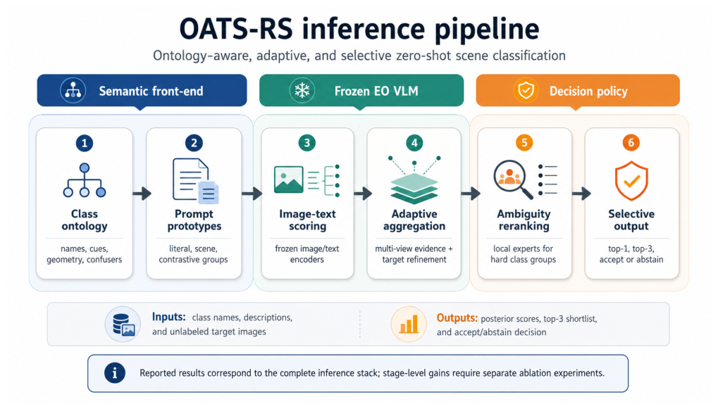
Figure 1. High-level schematic of OATS-RS. A frozen GeoRSCLIP/RemoteCLIP-style backbone is paired with ontology-aware prompt banks, hierarchical and contrastive scoring, adaptive multi-view aggregation, unlabeled target refinement, ambiguity-group re-ranking, and selective prediction. The manuscript analyzes the final output of the complete inference stack; stage-level gains require separate ablation experiments.
Remotesensing 18 02038 g001
Figure 2. (a) Top-line performance summary. (b) Bootstrap means and 95% intervals. Overall benchmark behavior of OATS-RS. The method achieves 0.522 top-1 accuracy and 0.887 top-3 accuracy, while the expected calibration error remains elevated.
Remotesensing 18 02038 g002
Figure 3. (a) Per-class precision, recall, and F1. (b) F1 ranking by class. Class-wise behavior of OATSRS. The metric spread is wide, with particularly strong performance on industrial area, residential area, river, highway, and pasture and very weak performance on herbaceous vegetation.
Remotesensing 18 02038 g003
Figure 4. Compact metric heatmap for the class-wise evaluation. The visualization makes the same asymmetry visible in a denser form: urban and river-related classes occupy the high-score corner, while several vegetation classes remain jointly weak across precision, recall, and F1.
Remotesensing 18 02038 g004
Figure 5. Qualitative examples of OATS-RS predictions: (a) representative correct predictions, including structured industrial area scenes and distinctive sea or lake scenes; (b) representative misclassifications, including industrial area → residential area, sea or lake → herbaceous vegetation, annual crop → permanent crop, and forest → herbaceous vegetation; and (c) dominant confusion pairs among semantically adjacent natural classes, especially forest, herbaceous vegetation, and pasture. The examples illustrate that the model is more reliable for structured or visually distinctive classes, while the strongest errors occur among vegetation-related categories with similar visual appearance.
Remotesensing 18 02038 g005
Figure 6. (a) Risk–coverage behavior. (b) Selective versus nonselective metrics. Selective prediction behavior of OATS-RS. Abstention modestly improves accuracy on accepted examples at high coverage, consistent with the elevated calibration error.
Remotesensing 18 02038 g006
Figure 7. Performance aggregated by coarse semantic family. The main gap is between urban/transport scenes and agriculture/vegetation scenes, not between human-made and water-related scenes.
Remotesensing 18 02038 g007
Figure 8. (a) Predicted labels on the annual crop diagnostic subset. (b) Confidence by correctness. (c) Margin by correctness. Local diagnostic analysis for annual crop based only on the supplied prediction diagnostics subset. Confusion is dominated by permanent crop, while the confidence and margin distributions show only weak separation between correct and incorrect predictions.
Remotesensing 18 02038 g008
Figure 9. Top-1 versus top-3 behavior. The large gap indicates that many errors are local ranking errors rather than total semantic failures.
Remotesensing 18 02038 g009
Table 1. Minimum parameter-reporting protocol for reproducible OATS-RS experiments. The table provides label-free setting rules and the reason that each parameter matters.
Parameter FamilySetting Rule in a Strict Zero-Shot RunPurpose and Failure Mode Controlled
Prompt-group weights w g Fix before evaluation; normalize over groups; report literal, scene, definition, context, geometry, signature, contrastive, pairwise, and parent weights separately.Controls how much the classifier trusts class names, semantic descriptions, geometric cues, and confuser prompts. Poor reporting means that prompt gains cannot be reproduced.
Prompt aggregation temperature τ g Use one value per group or a single global value; do not tune on test labels; report whether aggregation is mean-like or max-like.Controls whether many prompts contribute smoothly or whether one high-scoring prompt dominates.
Negative-confuser weight λ neg Increase only if label-free diagnostics show improved margins without severe class-prior collapse; report the final scalar.Penalizes classes with confuser prompts that are highly compatible with the image. Excessive values can suppress genuinely ambiguous classes.
Hierarchy weight λ h Use a small fixed value when parent categories are reliable; set to zero if parent ontology is uncertain.Prevents fine-grained labels from outranking implausible coarse families.
View temperature τ v and weights α 1 , , α 4 Fix across datasets or select by view-agreement stability; report number and type of views.Controls adaptive multi-view fusion; unstable view weighting can amplify augmentations that accidentally raise confidence.
Alignment parameters ρ , p , β Report shrinkage strength, power exponent, and blending coefficient; use conservative shrinkage when target set is small.Controls target–covariance alignment while limiting numerical instability and over-whitening.
Transductive parameters τ a , γ , η , ξ Report assignment temperature, confidence exponent, prototype blend, and prior-correction step size; monitor class-prior entropy.Controls unlabeled prototype refinement; aggressive settings can collapse predictions into easy classes.
Selective threshold τ Report both target coverage and actual coverage; never report selective accuracy without coverage.Determines abstention behavior and analyst workload.
Table 2. Transfer evaluation protocol for stronger empirical revision. Only EuroSAT RGB is measured in the supplied artifacts; the other rows specify required follow-up experiments rather than new results.
DatasetTask TypeWhy It Matters for Transferability
EuroSAT RGB [9]Ten-class Sentinel-2 scene classificationCurrent measured benchmark; tests compact land use and land cover semantics.
AID [10]High-resolution aerial scene classificationTests transfer to aerial imagery with different scale, appearance, and urban-object detail.
NWPU-RESISC45 [11]Remote sensing scene classification with 45 classesTests a larger and more fine-grained scene taxonomy with many visually adjacent classes.
BigEarthNet/
BigEarthNet-MM [12,30]
Multi-label land cover taggingTests whether ontology-aware prompts extend beyond single-label scene recognition.
SEN12MS [13]Multimodal Sentinel-1/2 representation learningTests whether the method can be adapted to multimodal optical-SAR evidence.
Table 3. Minimum component ablation ladder for OATS-RS. Values are not filled here because the supplied artifacts contain only the full final run.
VariantComponents EnabledMetrics to Report
GeoRSCLIP baselineSingle or standard prompt; frozen backbone; no ontology, no refinement.Top-1, top-3, ECE
+ ontology promptsPrompt groups for name, definition, context, geometry, and signature.Same plus class F1
+ contrastive/confuser scoringAdds negative prompts and pairwise confuser margins.Same plus confuser errors
+ adaptive multi-viewAdds view scoring and weighted view aggregation.Same plus throughput
+ target alignmentAdds covariance-shrinkage feature alignment on unlabeled target embeddings.Same plus stability
+ balanced transductive refinementAdds soft assignments, prototype updates, and class-prior correction.Same plus prior entropy
+ prompt support adaptationAdds high-confidence support centroids and drift control.Same plus support size
+ ambiguity expertsAdds local re-ranking for vegetation, water, or other confuser groups.Same plus local errors
Full OATS-RSAdds candidate ensembling and selective prediction.Same plus coverage/risk
Table 4. Fair comparison protocol. The current manuscript cites these families but does not report unsupported numerical comparisons.
Method FamilyFair-Use RequirementNotes for Interpretation
CLIP/OpenCLIP [2,4]Same RGB preprocessing and same prompt set when possible.Tests general VLM transfer without remote-sensing adaptation.
RemoteCLIP [34]Same split and image resolution; no target-label tuning.Tests remote sensing VLM pretraining under matched inference rules.
GeoRSCLIP/RS5M [35]Same checkpoint, preprocessing, and class names.Natural backbone baseline for the current method.
TPT/test-time prompt tuning [24]Report unlabeled-batch assumption and optimization steps.Useful but may differ from frozen-prompt inference.
Tip-Adapter/CLIP-Adapter [23,25]Clearly state whether labeled support examples are used.Few-shot variants are not strict zero-shot baselines.
SAM or SAM-assisted open-vocabulary pipelines [64,65,66,67]Convert masks to image-level labels or report dense metrics separately.Relevant for visual grounding, but not a direct scene-classification comparator without an aggregation rule.
Full OATS-RSSame backbone and target split as baselines; no target labels.Reports top-1, top-3, calibration, coverage, and class-wise diagnostics.
Table 5. Runtime and throughput metrics required for a complete reproducibility report. Values should be measured on the exact hardware used for evaluation.
MetricWhat to Report
Image encoder throughputImages per second for one view and for the full multi-view setting.
Text encoder costNumber of prompts, total prompt encoding time, and whether text embeddings are cached.
End-to-end throughputImages per second from image loading through final selective prediction.
Transductive overheadTarget-batch size, number of refinement iterations, nearest-neighbor cost, and additional seconds per batch.
Memory footprintPeak GPU memory or CPU memory for feature storage, covariance estimation, and neighbor search.
Hardware and softwareGPU/CPU model, precision, batch size, framework version, and backbone checkpoint.
Table 6. Experimental setting for the attached final evaluation.
ItemSetting
BenchmarkEuroSAT RGB
Label spaceTen scene classes
Model familyGeoRSCLIP
Backbone architectureViT-B-32
Training on target labelsNone (zero-shot)
Inference modePrompt-based zero-shot with adaptive selective inference
Input modalityRGB remote-sensing scene patches
Primary summary metricsAccuracy, balanced accuracy, macro-F1, micro-F1, top-3 accuracy, expected calibration error, coverage, selective accuracy
Empirical basis used in this paperFinal attached performance artifacts only
Table 7. Overall performance of OATS-RS on EuroSAT RGB using the attached final result files. Confidence intervals are reported only for metrics available in the bootstrap summary.
MetricValue95% Bootstrap CI
Accuracy0.5220.501–0.544
Balanced accuracy0.5220.505–0.539
Macro-F10.5350.520–0.550
Micro-F10.522
Expected calibration error0.3840.364–0.406
Top-3 accuracy0.8870.874–0.899
Coverage0.934
Selective accuracy0.538
Selective Macro-F10.548
Effective accuracy0.502
Table 8. Per-class precision, recall, and F1 on the attached EuroSAT RGB evaluation. Classes are ordered by F1 from strongest to weakest.
ClassPrecisionRecallF1
Industrial Area0.9240.9100.917
Residential Area0.8760.9550.914
River0.9660.8450.901
Highway0.9220.7700.839
Pasture0.8250.8000.812
Annual Crop0.2670.2500.258
Sea or Lake0.3470.2050.258
Forest0.1970.2650.226
Permanent Crop0.2060.1950.201
Herbaceous Vegetation0.0170.0250.021
Table 9. Representative operating points extracted from the attached risk–coverage curve. Risk is 1 Acc sel .
Target CoverageActual CoverageRiskSelective AccuracyThreshold
0.2500.2500.4700.5300.147
0.5000.5000.4060.5940.138
0.7500.7500.4370.5630.130
0.9000.9000.4530.5470.124
0.9340.9340.4620.5380.122
0.9500.9500.4660.5340.120
Table 10. Group-averaged precision, recall, and F1 derived from the attached per-class result table.
Semantic FamilyMean PrecisionMean RecallMean F1
Agriculture/vegetation0.3030.3070.304
Urban/transport0.9070.8780.890
Hydrographic0.6570.5250.580
Table 11. Summary of the attached annual crop diagnostic subset. This file appears to contain only annual crop ground-truth examples, so the table should be interpreted as a local error analysis rather than a global benchmark summary.
QuantityValueNotes
Subset accuracy0.250Matches Annual Crop recall
Prediction share: Permanent Crop0.650Dominant confusion mode
Prediction share: Sea or Lake0.055Secondary error mode
Prediction share: Herbaceous Vegetation0.025Rare error mode
Prediction share: Pasture0.020Rare error mode
Mean confidence (correct)0.143Std. dev. 0.008
Mean confidence (incorrect)0.131Std. dev. 0.006
Mean margin (correct)0.010Top-1 minus top-2
Mean margin (incorrect)0.012Top-1 minus top-2
Disclaimer/Publisher’s Note: The statements, opinions and data contained in all publications are solely those of the individual author(s) and contributor(s) and not of MDPI and/or the editor(s). MDPI and/or the editor(s) disclaim responsibility for any injury to people or property resulting from any ideas, methods, instructions or products referred to in the content.