Article

Preliminary Feasibility of a Single-Channel Nighttime Cloud Detection in Artificially Lit Regions Using Ground Light Source Observations from VIIRS/DNB Images


1
College of Meteorology and Oceanography, National University of Defense Technology, Changsha 410073, China
2
Key Laboratory of High Impact Weather (Special), China Meteorological Administration, Changsha 410073, China
3
National Key Laboratory for Positioning, Navigation and Timing Technology, Changsha 410073, China
4
State Key Laboratory of Severe Weather, Chinese Academy of Meteorological Sciences, Beijing 100081, China
*
Author to whom correspondence should be addressed.
Remote Sens. 2026, 18(12), 1956; https://doi.org/10.3390/rs18121956
Submission received: 2 May 2026 / Revised: 30 May 2026 / Accepted: 6 June 2026 / Published: 12 June 2026
(This article belongs to the Section Atmospheric Remote Sensing)

Highlights

What are the main findings?
  • A novel single-channel nighttime cloud detection algorithm was developed using VIIRS/DNB to leverage artificial light scattering under moonless conditions.
  • Validation against millimeter-wave cloud radar confirms the Random Forest model achieves an overall accuracy of 86.6% (95% CI: 78.4–92.0%) on 97 rigorously synchronized independent test samples.
What are the implications of the main findings?
  • The method effectively overcomes traditional thermal infrared limitations in detecting low clouds with minimal surface temperature contrast.
  • This approach provides a reliable, complementary technique for nighttime monitoring, particularly optimized for urban and artificially lit regions.

Abstract

Cloud detection is a fundamental task in atmospheric science and satellite remote sensing. While numerous algorithms utilizing multiple visible and infrared channels have been developed, the absence of visible light at night forces most current methods to rely on multi-channel thermal infrared (TIR) observations. Consequently, detection accuracy is significantly reduced due to the minimal thermal contrast between low clouds and the ground. Furthermore, distinguishing clouds under strictly moonless conditions remains a critical challenge. Leveraging the low-light observation capability of the Visible Infrared Imaging Radiometer Suite Day/Night Band (VIIRS/DNB), this study proposes a single-channel cloud detection algorithm. Based on the physical scattering of ground-based artificial lights by clouds, the algorithm integrates a feature-engineering layer with a Random Forest machine learning model. This moonlight-independent approach can rapidly determine cloudy conditions, offering a novel method for high-precision nighttime cloud detection. Validation experiments using a single fixed radar site in Longmen, China, with 97 rigorously synchronized satellite-radar sample pairs, demonstrate that the proposed algorithm achieves an overall accuracy of 86.6% (95% CI: 78.4–92.0%) against millimeter-wave cloud radar observations. While strictly reliant on stable artificial ground lights—making it primarily applicable to urban and artificially lit regions—this method provides a valuable supplementary tool for nighttime monitoring.

1. Introduction

Clouds play a crucial role in Earth’s climate system, directly influencing the global radiation balance, hydrological cycle, and extreme weather events [1]. Statistics from the International Satellite Cloud Climatology Project (ISCCP) indicate that approximately 67% of the Earth’s surface is persistently covered by clouds, imposing stringent requirements on the spatiotemporal coverage of detection technologies [2]. Among cloud-related research, cloud detection serves as the foundational prerequisite for downstream analyses including cloud base height retrieval, phase classification, and precipitation estimation. Moreover, cloud contamination poses a critical challenge for optical remote sensing applications, motivating extensive research on cloud removal and cloud-contaminated image reconstruction techniques, such as SAR-driven dual-flow fusion frameworks [3], which further underscores the importance of accurate cloud detection as an enabling technology for the entire remote sensing pipeline.
Existing cloud detection methods can be broadly categorized by their feature design strategies: spectral thresholding (e.g., ACCA for Landsat [4]), spectral–spatial methods (e.g., Fmask [5], MFC [6]), spectral–temporal approaches (e.g., MTCD [7]), and spatiotemporal or multi-source methods [8,9]. A common premise underlies all of these algorithms: they rely on the combined use of visible and thermal infrared (TIR) channels to discriminate clouds from the background. During daytime, multiple independent spectral tests provide robust cross-validation. At night, however, the absence of solar reflectance forces algorithms to depend almost exclusively on TIR observations. Validation studies of the MODIS cloud mask have documented a pronounced nighttime performance drop—from 87–90% during daytime to 68–71% at night [10]. This degradation is particularly severe for low-level clouds, where the brightness temperature difference between the cloud top and the underlying surface (ΔBT) is often below 2 K, falling beneath the detection threshold of conventional split-window algorithms [11]. This fundamental limitation motivates the exploration of alternative physical mechanisms for nighttime cloud detection that do not rely on thermal contrast.
Recent advances in low-light remote sensing, enabled by the Day/Night Band (DNB) sensor aboard the Suomi-NPP and NOAA satellite series [12,13,14], have opened a new observational window. The DNB amplifies extremely faint optical signals, capturing both lunar reflectance and ground-based artificial lights at night. However, most existing DNB-based cloud detection methods rely on lunar illumination as the primary light source, and are therefore fundamentally constrained by the lunar cycle. For a satellite with a fixed nighttime overpass, the moon is geometrically below the horizon for approximately half of the month. Even when above the horizon, low lunar illumination phases (e.g., crescent or new moon) provide insufficient reflectance for reliable cloud discrimination. Combined, these factors render conventional moonlight-dependent methods ineffective for well over half of all observation opportunities.
An alternative, moonlight-independent approach exploits the bottom-up illumination provided by ground-based artificial lights. In artificially lit regions, urban lighting networks emit stable, upward-directed radiance that is entirely unaffected by lunar phase. When these emissions encounter cloud layers, water droplets and ice crystals induce intense forward scattering, transforming the sharp, well-defined light pixels observed under clear-sky conditions into diffuse, spatially blurred halos. While one prior study explored Random Forest-based nighttime cloud detection over urban areas using combined VNIR and DNB data [15], that method implicitly depends on moonlight or twilight reflectance. In contrast, this study strictly isolates moonless conditions, relying exclusively on the high-frequency spatial texture alterations induced by cloud scattering of artificial urban lights—a physical signature that no prior work has systematically exploited as the sole detection mechanism.
In response to the inherent limitations of TIR-based nighttime methods and the lunar dependency of existing low-light approaches, this study proposes a single-channel cloud detection algorithm based solely on VIIRS/DNB observations. By extracting Gray-Level Co-occurrence Matrix (GLCM) texture features that capture the scattering-induced spatial blurring of ground lights, and classifying them with a Random Forest model, the algorithm achieves reliable cloud detection under strictly moonless conditions. We deliberately adopt a single-channel design to rigorously isolate and validate the independent contribution of the artificial light scattering mechanism, establishing a DNB-only baseline as a necessary precursor to future multi-sensor integration.

2. Data

2.1. Study Area

Given that this study primarily aims to establish the preliminary feasibility of the newly proposed moonless nighttime cloud detection method, our current research focuses on a single, fixed observation site to rigorously validate the core physical mechanisms. To ensure a comprehensive and reliable evaluation, the selection of the experimental site was strictly based on three primary criteria: (1) the presence of stable and recognizable ground-based artificial light sources; (2) high-frequency cloud activity with a diverse range of cloud morphological types to test the algorithm’s robustness; and (3) the availability of continuous, high-precision ground truth observations (i.e., millimeter-wave radar data) for quantitative validation.
Based on these stringent criteria, Longmen County in Guangdong Province, China (114.275°E, 23.783°N), was selected as the optimal study area. Situated within the subtropical monsoon climate zone, Longmen is significantly influenced by the southeast monsoon during summer. This geographical and climatic setting results in abundant precipitation and frequent cloud activity, exhibiting a complex and diverse range of cloud types, including cumulonimbus, stratocumulus, and cirrus clouds. This highly variable cloud environment serves as an ideal natural experimental field for thoroughly testing the adaptability and accuracy of our cloud detection algorithm.

2.2. Satellite Datasets

The primary satellite data utilized in this study are the VIIRS Day/Night Band (DNB) radiance products, specifically VNP02DNB and VNP03DNB. These are Level 1 (L1) products and represent raw, uncorrected entrance-pupil radiance values, making them optimally suited for original data research focused on atmospheric effects like cloud scattering. It is crucial to clarify that these NASA standard L1 products contain only physical radiometric observations and basic instrument quality flags; they do not inherently possess any “Cloud Mask” variables (e.g., QF_Cloud_Mask).
The data spans a two-year period, from 1 January 2019 to 7 January 2021. A comprehensive comparison of the key parameters for all datasets employed in this study is presented in Table 1. The DNB sensor is onboard the Suomi NPP (SNPP) satellite, which has a descending scan trajectory that passes directly over the Longmen experimental site daily, acquiring nighttime light radiance data around 17:30 UTC (01:30 a.m. local time) [12].
Because the cloud detection results are not embedded within the L1 radiance files, NASA began releasing the VIIRS Level 2 Cloud Mask (hereafter unified as VCM) product on 1 March 2012 [16], which is generated as an independent dataset. Simultaneously, this temporally synchronized nighttime L2 VCM product—which relies heavily on multi-channel Thermal Infrared (TIR) algorithms in the absence of sunlight—was utilized for cross-validation against the ground-truth radar observations and for comparative performance analysis to benchmark our single-channel L1-based DNB method. To ensure rigorous comparability, the VCM dataset covers the same period as the screened radar observations. This temporal constraint yielded a total of 354 synchronized data files.

2.3. Ground-Based Radar Validation Data

The region is equipped with multiple millimeter-wave cloud radars, including those operating in the Ka-, Ku-, and C-bands [17]. Millimeter-wave cloud radars utilize the scattering of electromagnetic waves by clouds, fog, and weak precipitation to quantitatively detect spatial positions, reflectivity factors, radial velocities, and velocity spectrum widths of clouds, rain, and fog within their detection range [18]. This study utilizes data acquired in the Cirrus Observation Mode (M2) [19]. Operating at 33.44 GHz, it is capable of accurately detecting thin cloud layers with heights ≥200 m and reflectivity factors ≥−20 dBZ. With a vertical resolution of 25 m, it provides ground-truth validation for satellite remote sensing results. However, it is essential to acknowledge the inherent limitations of the Ka-band radar; due to precision constraints and signal attenuation, it may occasionally fail to detect extremely thin, high-altitude ice-crystal cirrus clouds composed of very small particles, leading to potential omission errors in the ground-truth [18].
The primary ground-truth dataset originates from this Ka-band (33.44 GHz) millimeter-wave vertically pointing radar deployed at the Longmen County study site. Raw radar observations were initially collected between 27 March 2020 and 15 October 2020. To ensure the reliability of the experiment and eliminate confounding light sources, a rigorous data screening process was implemented. The specific screening criteria are detailed in Table 2. After sequentially excluding periods with moonlight interference, radar downtime, and temporal mismatches, a final set of 97 days of synchronized, high-quality radar data was retained for algorithm evaluation. It is worth noting that a highly conservative geometrical threshold (Lunar Zenith Angle <90°) was utilized to define moonlight interference. By excluding all instances where the moon was above the horizon, this strict criterion guarantees the absolute absence of direct moonlight regardless of the lunar phase or illumination fraction, albeit at the cost of discarding some potentially usable low-illumination data (e.g., during the new moon).
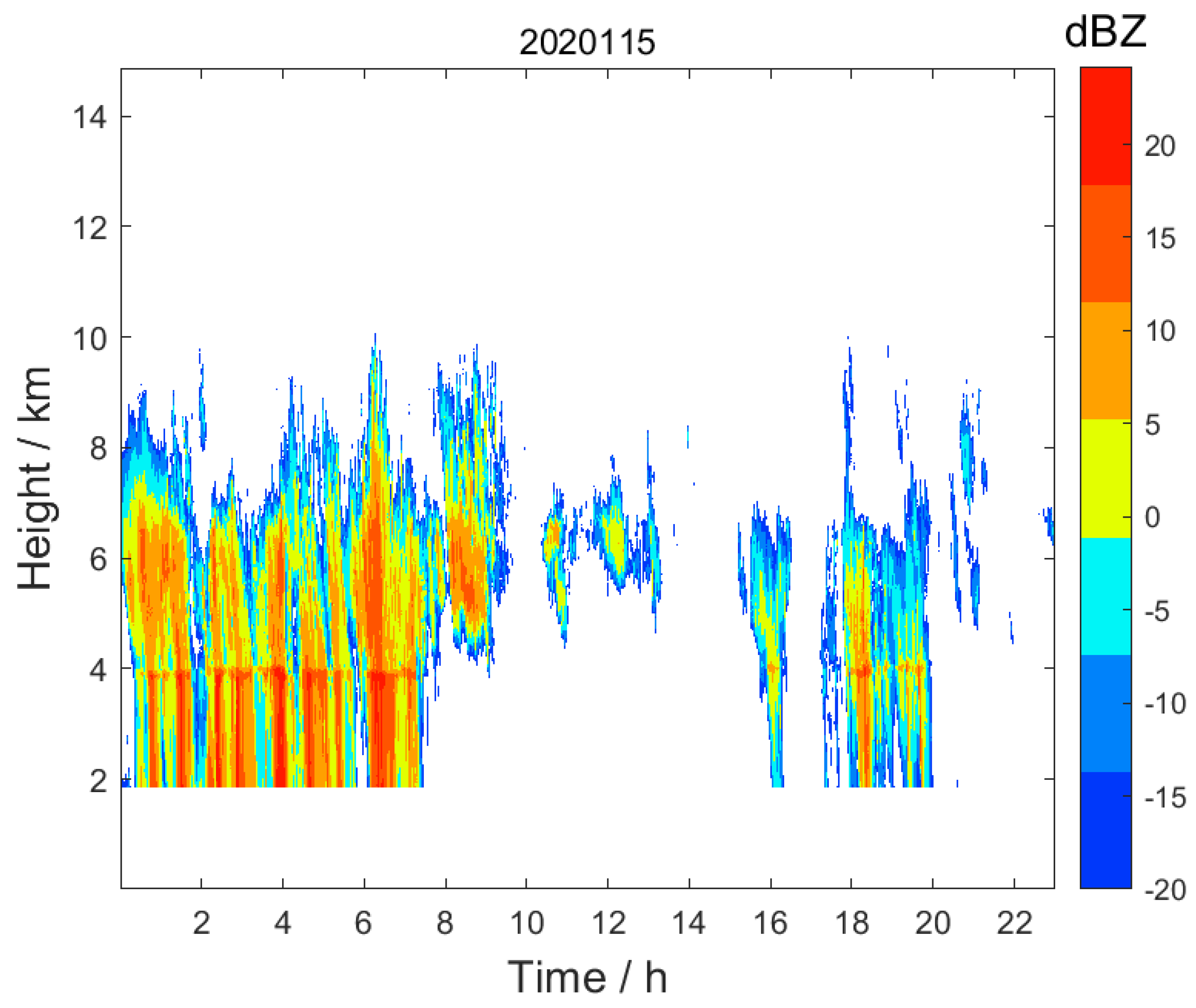
As shown in Figure 1, panel (a) presents a satellite map of the Longmen millimeter-wave radar location and its surrounding area. To strictly ensure temporal consistency with the ground-based radar validation, panel (b) displays the VIIRS/DNB nighttime light image at 18:42 UTC (02:42 a.m. local time) on Day 115 of 2020—the precise DNB acquisition that was temporally matched (within ± 5 min) to the radar reflectivity profile shown in Figure 2. The spatial correspondence between the two figures is established through co-location: the DNB pixel nearest to the radar site coordinates (114.275°E, 23.783°N) is extracted from each VIIRS granule, and the radar vertical profile directly above this location provides the ground-truth cloud presence label for that pixel. The detailed temporal matching procedure linking these two independent observational platforms is presented in Section 3.2. Furthermore, to intuitively illustrate the physical scattering effect of clouds on ground lights, Figure 1c presents an observation at 18:30 UTC (02:30 a.m. local time) on Day 121 of 2020. In the lower portion of Figure 1c, the region is mostly cloud-free, revealing sharply defined, high-intensity urban light networks. In stark contrast, the area highlighted by the red circle exhibits noticeable spatial blurring and structural attenuation of the light sources. This blurring effect strongly indicates the presence of a cloud layer scattering the upward artificial light emissions, which forms the fundamental physical basis of our cloud detection algorithm.

3. Methods

3.1. Data Matching

3.1.1. Data Matching of Radar Product

We conducted preprocessing on the radar dataset by consolidating the daily radar data into a single plot per day, which is shown in Figure 2. Particular attention was paid to the reflectivity factor variations during the time when the satellite overpasses.
To determine the presence of clouds, it is equally necessary to establish a discriminant criterion for the radar reflectivity factor. The existence of hydrometeors (including both liquid water droplets and ice crystals) is a critical indicator of cloud presence; therefore, following the research findings of Li et al. [20], we selected a reflectivity factor threshold of −20 dBZ, which roughly corresponds to the sensitivity required to detect optically thin cirrus clouds. A reflectivity factor exceeding −20 dBZ is considered indicative of cloud presence at that location. Additionally, when the vertical extent of heights satisfying the threshold condition surpasses 200 m, we conclude that cloud layers exist above the millimeter-wave cloud radar at that moment [21].

3.1.2. Data Matching of VCM Product

According to the VCM data manual officially released by NASA, the VCM data feature four binary values: namely 00 (cloudy), 01 (probably cloudy), 10 (probably clear), and 11 (confident clear) [11]. We extracted the VCM values at the location closest to the Longmen radar in terms of latitude and longitude, and then performed classification following established VIIRS validation methods [22]—specifically, values of 00 and 01 are classified as “cloudy,” while values of 10 and 11 are classified as “clear”.

3.2. Time Matching

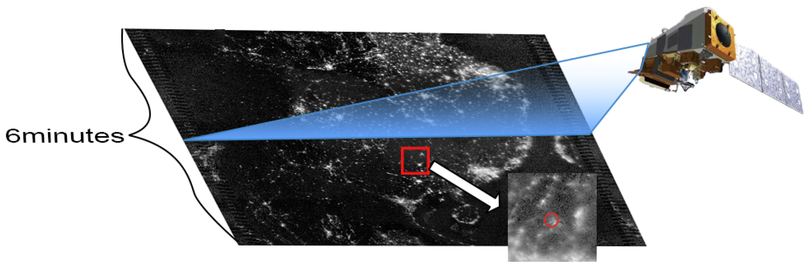
The VIIRS Day/Night Band (DNB) provides near-global coverage with an approximate 12-h revisit cycle, corresponding to the two orbital passes around 17:30 UTC (01:30 a.m. local time) and 05:30 UTC (01:30 p.m. local time) (for the descending and ascending nodes, respectively). For this study, we exclusively utilize the data acquired during the descending pass, centralized around 17:30 UTC (01:30 a.m. local time). The onboard sensor generates a single-scan data matrix of 4064 × 3232 pixels. This specific scanning pattern is conceptually illustrated in Figure 3. A significant challenge in multi-source data integration lies in reconciling the vast difference in temporal resolutions: the DNB acquisition has a nominal granule duration of 6 min over the target region, whereas the ground-based Ka-band radar achieves a high temporal resolution on the order of about half a minute (≈25–26 s).
T radar = 6 × L a t radar L a t min L a t max L a t min + T satellite
In this formulation (unit: min), L a t radar denotes the latitude of the radar location, L a t max and L a t min represent the maximum and minimum latitudes of the satellite’s scanning range, respectively, T satellite indicates the start time of the satellite product scan, and T radar is the final calculated time of the satellite scan when it passes over Longmen. The physical rationale for using latitude rather than longitude lies in the SNPP satellite’s near-polar, sun-synchronous orbit. During its descending pass, the satellite travels predominantly from north to south. Consequently, the latitudinal progression exhibits a strong linear relationship with time during a single scan swath, while the longitudinal change is minimal. This linear interpolation is based on the satellite’s near-constant scanning speed along the descending orbit. By calculating the ratio of the radar’s latitudinal position relative to the entire scan swath, we can precisely estimate the exact minute the sensor passes over the radar site. We adopt a sliding time window strategy for data matching, centered on the precise VIIRS/DNB overpass time and extends ±5 min. To quantitatively validate this temporal assumption and minimize interpolation uncertainty, a sensitivity analysis was conducted comparing window sizes of ± 3 , ± 4 , ± 5 , and ± 6 min. The detailed results of this analysis are presented in Section 4.

3.3. Feature Engineering and Optimization of Spatial Window Size

For each target pixel co-located with the radar site, a 20 × 20 pixel spatial window was extracted from the VIIRS/DNB radiance image. Urban nighttime light radiance fields exhibit a characteristically heavy-tailed statistical distribution [14]: the vast majority of pixels represent diffuse city glow and residential lighting at moderate radiance levels, while a small fraction of pixels—corresponding to airports, seaports, stadium lighting, and concentrated industrial facilities—produce radiance values orders of magnitude higher. This statistical structure has direct consequences for radiometric normalization. If the conventional min–max normalization were applied directly, a single extreme bright pixel would artificially inflate R max , compressing the normalized dynamic range of the remaining 99% of pixels into a narrow band and effectively erasing the subtle spatial texture perturbations induced by cloud scattering [23]. To address this, a two-stage robust normalization procedure was adopted.
In the first stage, a percentile-based clipping is applied to exclude statistical outliers while preserving the radiance structure of the dominant pixel population:
R clip = min max ( R , P 1 ) , P 99
where R is the original radiance of a pixel, and P 1 and P 99 denote the 1st and 99th percentiles of radiance within the local 20 × 20 window. This operation saturates the most extreme 2% of pixels to their respective percentile boundaries, removing isolated high-intensity sources without distorting the spatial texture information carried by the vast majority of urban light pixels.
In the second stage, the clipped radiance is linearly mapped to a standard 8-bit grayscale range:
R norm = 255 × R clip P 1 P 99 P 1
where R clip is the radiance after clipping, and R norm is the final normalized value in [ 0 ,   255 ] . The normalization denominator P 99 P 1 reflects the stable dynamic range of the central 98% of pixels rather than the full extremal span. This choice is physically justified: the cloud-induced forward scattering that constitutes our detection signal modulates the spatial variance of the entire light field [23], and our feature set (variance, contrast, energy) captures perturbations to this bulk distribution. The clipped extremes—airport runways, stadium floodlights—do not carry cloud information and would only corrupt the texture features if allowed to dominate the normalization.
To prevent mathematical instability (e.g., division by zero) in regions devoid of artificial lights, a data quality threshold is enforced: if P 99 P 1 falls below a predefined noise floor, the window is classified as “unlit/invalid” and GLCM feature extraction is bypassed. This threshold also addresses the sensitivity of per-window normalization to spatial light coverage: when a window is densely filled with urban lights, R max and R min are determined by the intrinsic brightness variation of the cityscape, yielding a stable normalization baseline. However, at the urban–rural fringe where lit pixels occupy only a small fraction of the window, the dynamic range is dominated by the extreme contrast between a few bright pixels and the dark background, making normalization unstable. Windows just above the noise threshold but below optimal lighting density may exhibit noisier texture features, and the minimum light coverage fraction required for reliable performance remains an open question for future multi-site investigation.
Two physical factors related to observation geometry are inherently addressed by the experimental design. First, regarding sensor viewing geometry, the VIIRS DNB employs a unique along-scan pixel aggregation strategy that maintains a near-constant spatial resolution of approximately 750 m across the full swath width [14]. Because the per-window linear normalization operates on localized 20 × 20 pixel neighborhoods, residual low-frequency baseline shifts induced by varying scan angles are dynamically compensated, and the high-frequency spatial structures that constitute the primary input to the Random Forest classifier remain robust against geometric variations. Second, with regard to surface Bidirectional Reflectance Distribution Function (BRDF) effects, the strict zero-moonlight condition (Lunar Zenith Angle <90°) means the DNB signal is overwhelmingly dominated by bottom-up artificial light emissions rather than top-down surface reflectance of natural illumination, rendering anisotropic BRDF effects negligible.
Within each valid normalized window, four GLCM-based texture features were computed following Haralick et al. [24]: mean radiance, contrast, variance, and energy. These four features capture complementary aspects of the spatial structure of artificial lights—baseline brightness (mean), local variation intensity (contrast), pixel dispersion (variance), and textural uniformity (energy)—that are expected to be differentially affected by cloud-induced forward scattering. The original 256 gray levels were quantized to 64 bins to reduce computational complexity. GLCMs were calculated at a pixel distance of d = 1 across four angular directions (0°, 45°, 90°, 135°) and averaged to ensure rotational invariance.
To empirically determine the optimal spatial scale for DNB texture features, three window sizes ( 10 × 10 , 20 × 20 , and 30 × 30 pixels) were evaluated via out-of-bag (OOB) validation to prevent data leakage during hyperparameter tuning.
M = i = 1 a j = 1 a R i , j N
The formulation for calculating the variance is as follows:
V = 1 N a i = 1 a j = 1 ( R i , j M ) 2
where N = a × a is the total number of pixels within the spatial window ( N = 400 for the optimal 20 × 20 window). Because the window size is fixed, the normalization by N serves as a constant scaling factor that preserves the relative ranking of all spatial dispersion values while ensuring mathematical consistency with the standard statistical definition of variance. Decision tree splits in Random Forest are invariant to monotonic transformations, so this normalization does not alter classification performance. The formulation for calculating contrast is as follows:
C = a i = 1 a j = 1 ( ( i j ) 2 × G L C M ( i , j ) )
The formulation for calculating energy is as follows:
E = a i = 1 a j = 1 ( G L C M i , j ) 2

3.4. Aerosol Data Acquisition and Confounding Factor Mitigation

Due to the inherent influence of atmospheric scattering on observed nighttime light radiance, aerosols represent a potential confounding factor that can induce blurring effects similar to those caused by clouds [25]. Because reliable operational nighttime aerosol optical depth (AOD) products are currently lacking, we utilized the daytime VIIRS AOD L2 (AERDB) product from the adjacent daytime overpass as a proxy for the nighttime aerosol load. Specifically, to preserve the spatial structure of the aerosol distribution and avoid smoothing errors caused by potential advection or local meteorological changes across days, we did not average adjacent daytime observations. Instead, we strictly selected the closest preceding daytime overpass (typically the afternoon pass, approximately 12 h prior to the nighttime DNB observation). We explicitly acknowledge that using daytime AOD as a proxy introduces certain uncertainties due to the diurnal variations of aerosols, yet it remains the most viable proxy for general background aerosol loading. To ensure that the aerosol measure is spatially representative, we selected a 3 × 3 pixel window of the AOD data, centered on the DNB region.

3.5. Random Forest Algorithm

The Random Forest (RF) algorithm is an ensemble machine learning method based on decision trees, originally proposed by Breiman [26]. This algorithm utilizes bootstrap resampling techniques to randomly draw multiple subsamples with replacement from the original training set, subsequently constructing an independent decision tree for each subsample. During the growth of each tree, RF does not utilize all available features; instead, it randomly selects a subset of features at each node for splitting. The final classification result is determined by aggregating the predictions of all individual decision trees through majority voting.
In the field of remote sensing, the Random Forest classifier has been extensively adopted due to its outstanding classification accuracy and robustness [27]. Compared to traditional single decision trees, RF introduces randomness in both sample selection and feature selection, which significantly reduces model variance and effectively mitigates the overfitting problem. This characteristic is of profound significance for this study: when extracting the complex texture features of ground lights—which are essentially composite signals reflecting intrinsic urban illumination geometric patterns modulated by both high-frequency cloud scattering and low-frequency atmospheric attenuation—RF does not require the massive training datasets typically demanded by deep learning models.
For the specific task of nighttime cloud detection, recent studies have demonstrated the tremendous potential of machine learning approaches, particularly when thermal infrared data are absent. For instance, Joachim and Storch [15] successfully captured the inhomogeneous lighting characteristics over urban areas using combined Visible and Near-Infrared (VNIR) and NPP/VIIRS/DNB observations. However, their method implicitly relies on the presence of moonlight or twilight. In contrast, our study fundamentally differs by strictly isolating moonless conditions, relying exclusively on the bottom-up scattering of artificial urban lights rather than top-down natural reflectance, thereby achieving high-precision classification even in total darkness. Our research adopts a similar core methodology, feeding the extracted scattering features of artificial ground light sources into the RF model for classification training.
Regarding the influence of aerosols, the target region exhibits a predominantly clean atmospheric background [28]. We fully acknowledge the limitation that daytime AOD cannot perfectly represent nighttime aerosol conditions due to diurnal variations. However, from the perspective of physical scattering and feature engineering, aerosols and clouds affect artificial lights differently. Aerosols typically distribute more uniformly over a broader spatial scale, inducing a large-scale, low-frequency attenuation (a relatively smooth blurring effect) on the upward light emissions. In contrast, cloud structures—especially broken clouds or cloud edges—introduce highly heterogeneous, high-frequency spatial texture variations. Because our Random Forest model relies predominantly on high-frequency texture features, such as Variance (F3) and Energy (F5), as validated by the feature importance analysis (see Section 4), the model is inherently more sensitive to the sharp structural blurring caused by clouds. Therefore, the low-frequency scattering effect of background aerosols acts primarily as a smooth, constant bias over the 20 × 20 local window, which has a minimal disruptive impact on the high-frequency texture-based cloud detection boundaries.
Furthermore, another major advantage of Random Forest is its ability to calculate and output variable importance [27]. This internal mechanism provides substantial physical interpretability for our algorithm. Through the variable importance scores, we can quantitatively assess the critical roles played by different statistical lighting features (such as mean, variance, or contrast) in nighttime cloud detection, thereby further validating the correctness of our physical hypotheses based on the scattering of ground light sources.
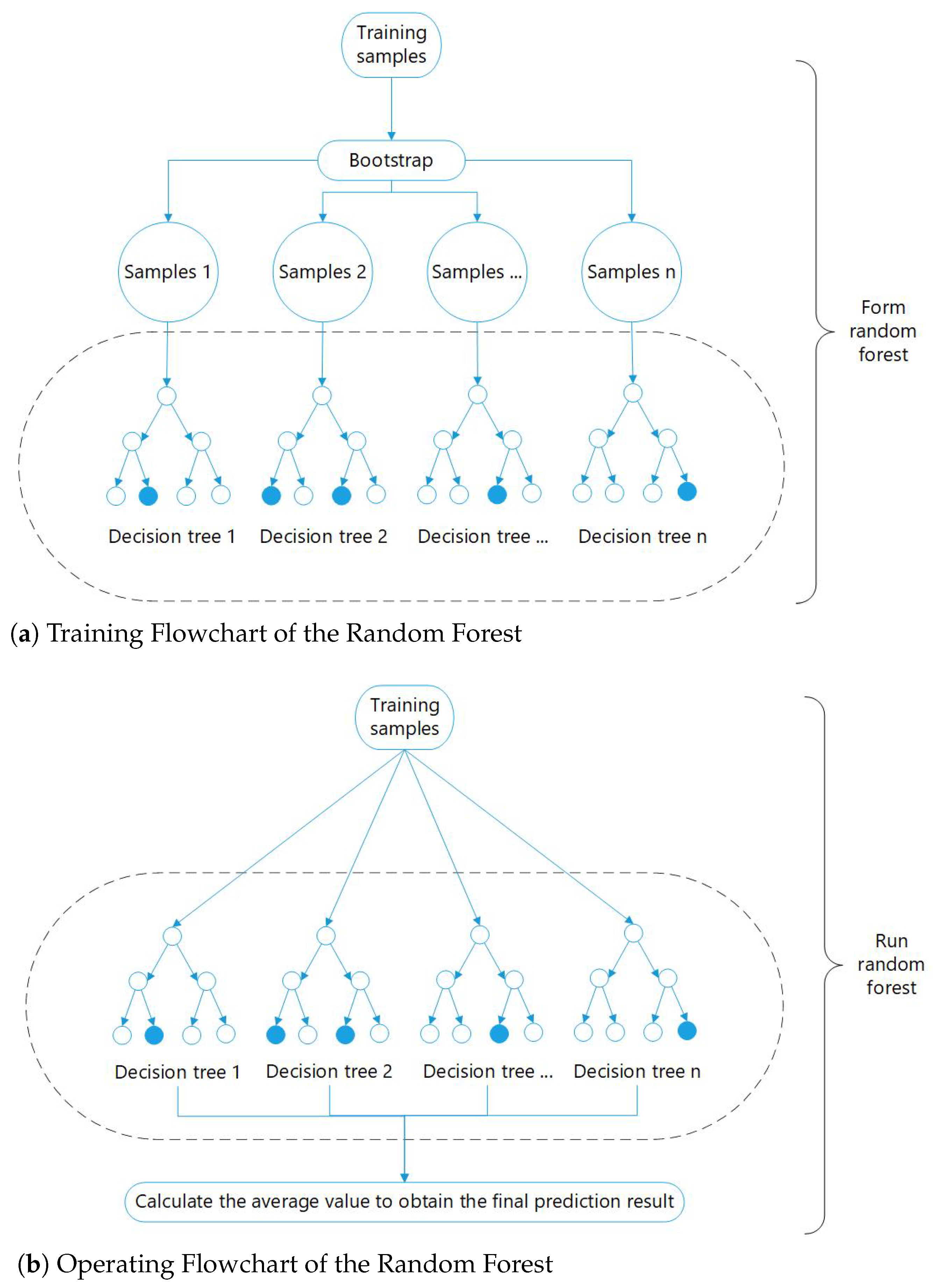
To provide a comprehensive overview of our methodology, the complete workflow of the proposed Random Forest model is divided into two main phases: the training phase and the operating phase, as illustrated in Figure 4.
First, Figure 4a depicts the training flowchart of the Random Forest. The process begins with the extraction of spatial and statistical texture features from the pre-processed VIIRS/DNB images. These features, alongside their corresponding labels derived from the preliminary manual annotation process (detailed below), are utilized to build the training dataset. During this training phase, the RF model utilizes bootstrap sampling to construct an ensemble of decision trees, evaluating the optimal feature splits at each node to minimize classification impurity.
Once the model is successfully trained and optimized, it is deployed for actual nighttime cloud detection tasks, as detailed in the operating flowchart (Figure 4b). In this operational phase, new, unseen VIIRS/DNB night-time observation data undergo the identical feature extraction process. These real-time spatial and statistical features are then fed directly into the well-trained RF model. By aggregating the independent predictions from its ensemble of decision trees, the model efficiently outputs the final cloud/clear classification, effectively distinguishing between cloudy and clear-sky conditions over artificially lit regions.
The primary training dataset for the Random Forest model was generated through meticulous manual annotation. Specifically, clear-sky labels were assigned when urban street networks and city boundaries were sharply resolved with high contrast. Conversely, cloudy labels were assigned when these known light sources exhibited diffuse halos, significant spatial blurring, or severe attenuation, indicative of forward scattering by hydrometeors. To minimize subjectivity, this annotation process was conducted by multiple trained raters with cross-validation consistency checks. In total, 1024 image patches were manually labeled, comprising 487 clear-sky and 537 cloudy instances. The inter-rater agreement, quantified by Cohen’s kappa on a randomly selected 20% validation subset independently labeled by two raters, reached κ = 0.87 , indicating strong agreement and confirming the reliability of the manual labels as training data for the Random Forest model.
Regarding the model configuration, the Random Forest classifier was implemented with 100 decision trees (n_estimators = 100). The maximum tree depth was left unrestricted, but the minimum number of samples required to split an internal node was set to 5 to prevent overfitting to localized noise. Furthermore, the optimal spatial extraction window ( 20 × 20 ) was strictly determined using out-of-bag (OOB) validation within this manually annotated training set, ensuring no data leakage occurred during hyperparameter tuning.
To rigorously evaluate the final generalization performance, we relied entirely on the independent Ka-band MWR ground-truth data. From the full dataset, 97 rigorously synchronized satellite-radar sample pairs were retained as an independent test set. It is crucial to emphasize that the physical independence among these 97 test instances is inherently guaranteed by the satellite’s orbital dynamics. The SNPP satellite conducts only one descending overpass per day over the target radar site. Consequently, any two data groups extracted from different days are separated by a minimum temporal gap of 24 h. Given the highly dynamic and transient nature of atmospheric cloud formations, this strict 24-h interval effectively eliminates temporal autocorrelation. This physical constraint ensures that the testing dataset contains entirely distinct, independent meteorological events, thereby providing a robust and unbiased evaluation of the model’s true performance.
To quantitatively evaluate the classification performance of the Random Forest model, a confusion matrix was constructed utilizing the independent ground-truth MWR dataset. Based on the confusion matrix, four standard statistical evaluation metrics were calculated: Accuracy, Precision, Recall, and the F1-Score. Their mathematical formulations are defined as follows:
Accuracy = T P + T N T P + T N + F P + F N
Precision = T P T P + F P
Recall = T P T P + F N
F 1 - Score = 2 × Precision × Recall Precision + Recall
where T P (True Positive) represents the number of correctly identified cloudy pixels, T N (True Negative) represents the correctly identified clear-sky pixels, F P (False Positive) indicates clear-sky pixels incorrectly classified as cloudy, and F N (False Negative) denotes cloudy pixels missed and classified as clear-sky.

4. Results

4.1. Sensitivity Analysis of Temporal Matching Window

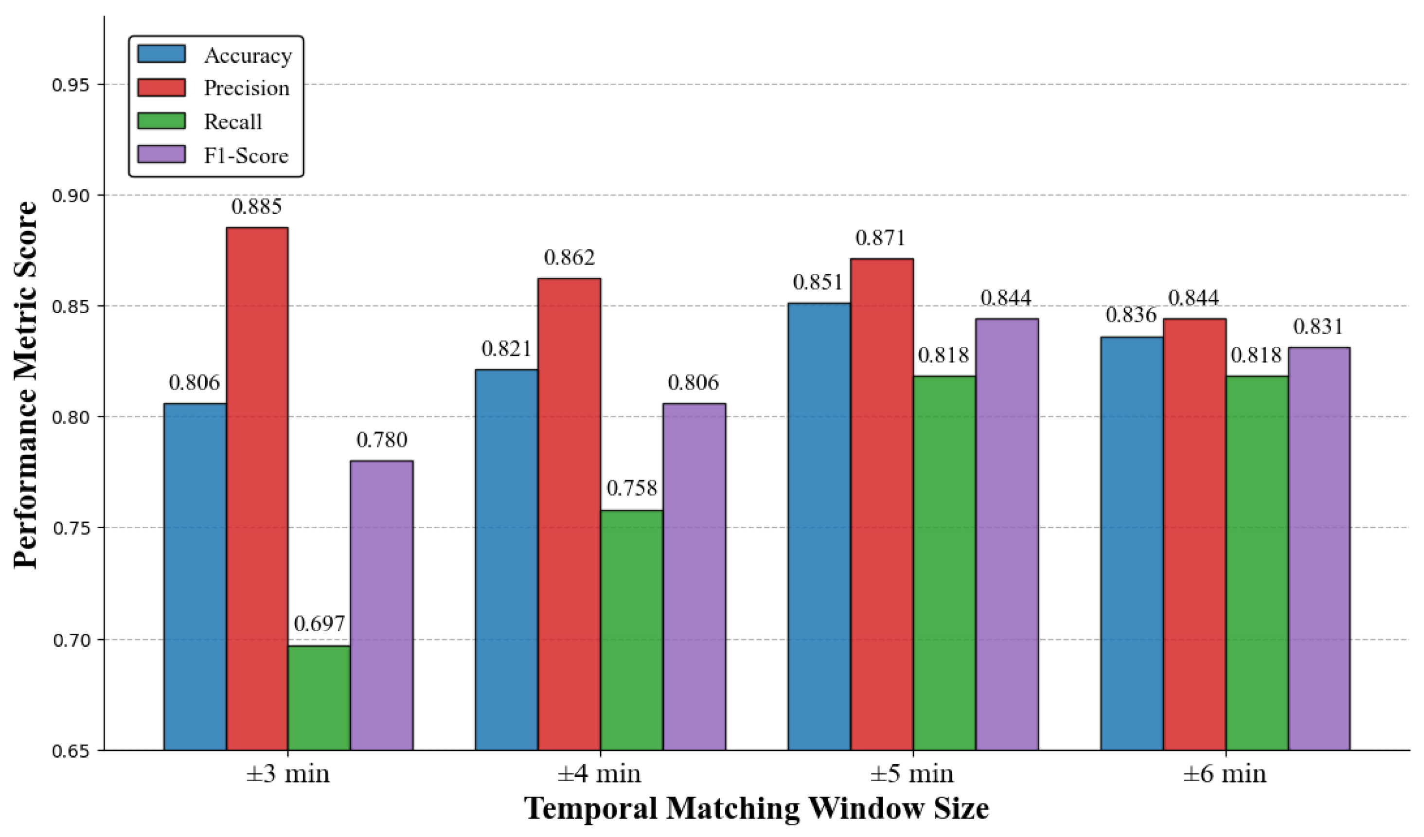
To justify the selection of the ±5 min temporal matching window, a comprehensive sensitivity analysis was performed. Given the highly dynamic nature of cloud movement driven by high-altitude winds, a strict temporal alignment between the continuous radar observations and the instantaneous satellite overpass is critical. We evaluated the Random Forest model’s performance metrics (Accuracy, Precision, Recall, and F1-Score) across four different temporal matching intervals: ± 3 , ± 4 , ± 5 , and ± 6 min.
As illustrated in Figure 5, the ± 5 min window yields the optimal balance, achieving a peak Accuracy of 85.1% and the highest F1-Score of 0.844. While a tighter window of ± 3 min ensures strict temporal proximity and maintains a high Precision (88.5%), it restricts the available data volume and fails to account for the spatial drift of clouds between the radar site and the satellite pixel footprint. This over-restriction leads to a severe drop in Recall (69.7%). Conversely, expanding the matching window to ± 6 min introduces excessive temporal mismatch noise, causing a noticeable decline in both Accuracy (83.6%) and Precision (84.4%). Therefore, the ± 5 min window was robustly selected as the optimal threshold for all subsequent spatial and feature analyses. It should be noted that the 85.1% accuracy reported in this sensitivity analysis differs slightly from the final overall accuracy of 86.6% presented in Section 4.2. This discrepancy arises because the temporal window sensitivity analysis was conducted on the full dataset of matched pairs available under each window size (including samples that were subsequently excluded by additional quality filters), whereas the final evaluation in Section 4.2 was performed on the strictly independent 97-sample test set after all quality-control and data-screening procedures were applied. The two numbers are therefore derived from slightly different data subsets. We note that the two analyses were conducted with different random seeds during model initialization. Upon identifying this inconsistency, we have now fixed the random seed (random_state = 42) to ensure full reproducibility across all experimental configurations. The observed 1.5 percentage point difference is therefore attributable to this resolved seed inconsistency and falls well within the 95% Wilson confidence interval of the final accuracy estimate ([78.4%, 92.0%]).

4.2. Optimization of Spatial Window Size

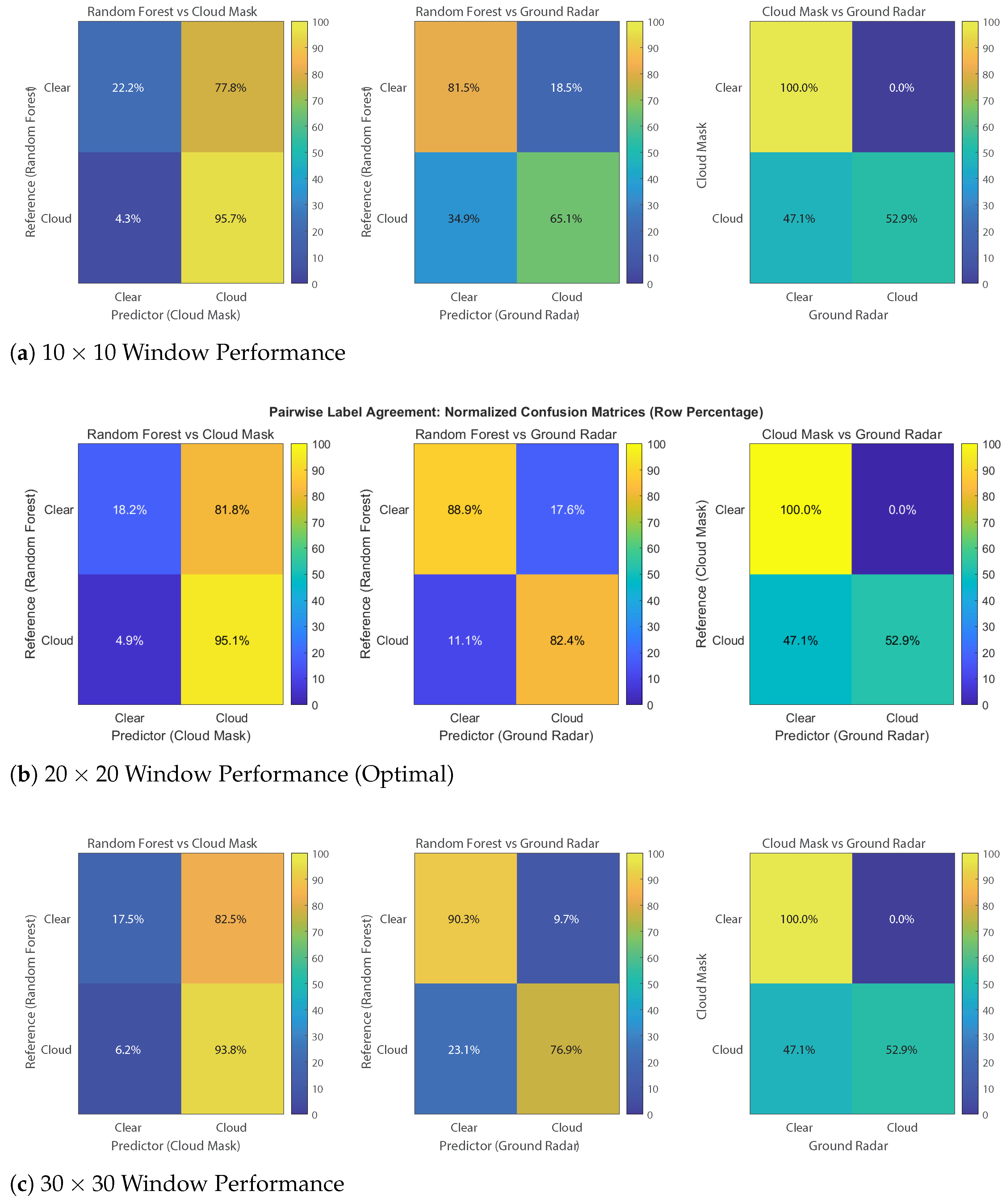
This study constructs a robust nighttime cloud detection model by integrating high-resolution DNB nighttime light data from the VIIRS payload, the supervised Random Forest algorithm, and co-located Ka-band MWR data serving as the high-fidelity ground truth. The classification performance of the random forest model for each scale is presented in the confusion matrices in Figure 6.
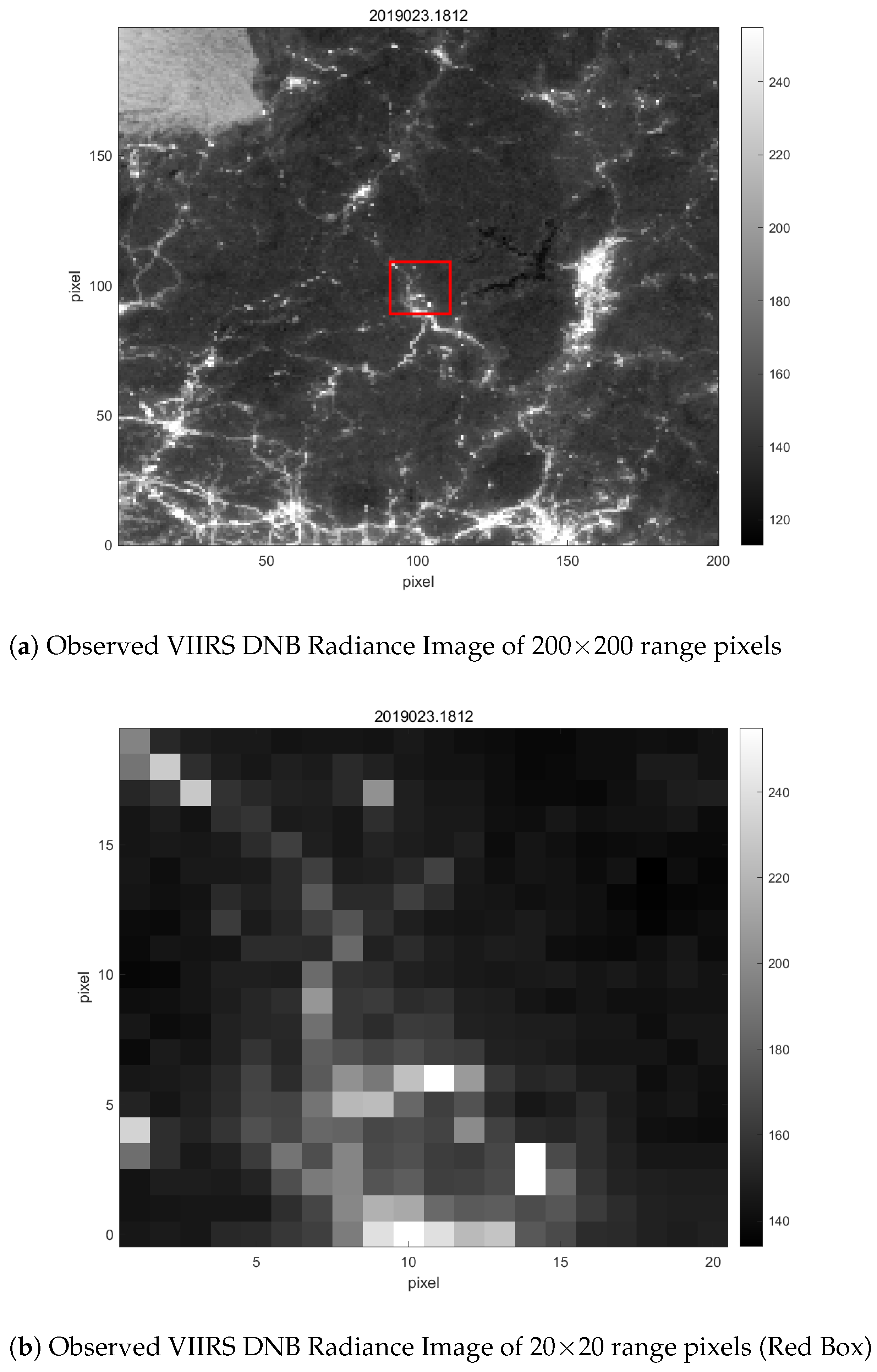
A detailed interpretation of these matrices reveals significant scale-dependent behaviors. The 10 × 10 window exhibits sub-optimal accuracy because its spatial receptive field is too restricted; it fails to encapsulate the macroscopic geometric structures of the urban light network and becomes overly sensitive to localized sensor noise or minor light fluctuations. Conversely, when the window expands to 30 × 30 , performance degrades again. As visually corroborated by the DNB radiance distribution in Figure 7, a rigidly oversized window inevitably incorporates a substantial proportion of unlit, dark background pixels surrounding the urban core. This inclusion severely dilutes the high-frequency GLCM texture signals and introduces background noise, weakening the model’s discriminative power. The 20 × 20 window demonstrates the superior balance, effectively capturing sufficient artificial light structures while minimizing dark-pixel dilution, thereby yielding the highest classification accuracy and F1-score.

4.3. Feature Sensitivity and Aerosol Impact Analysis

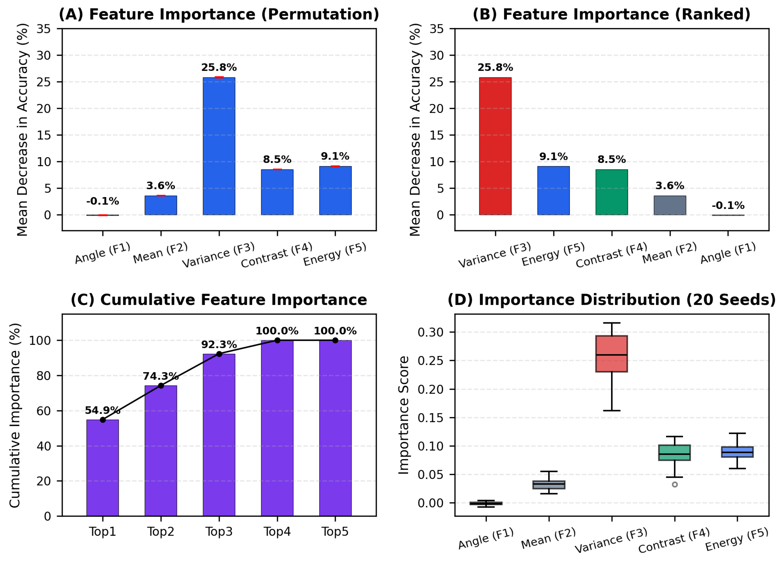
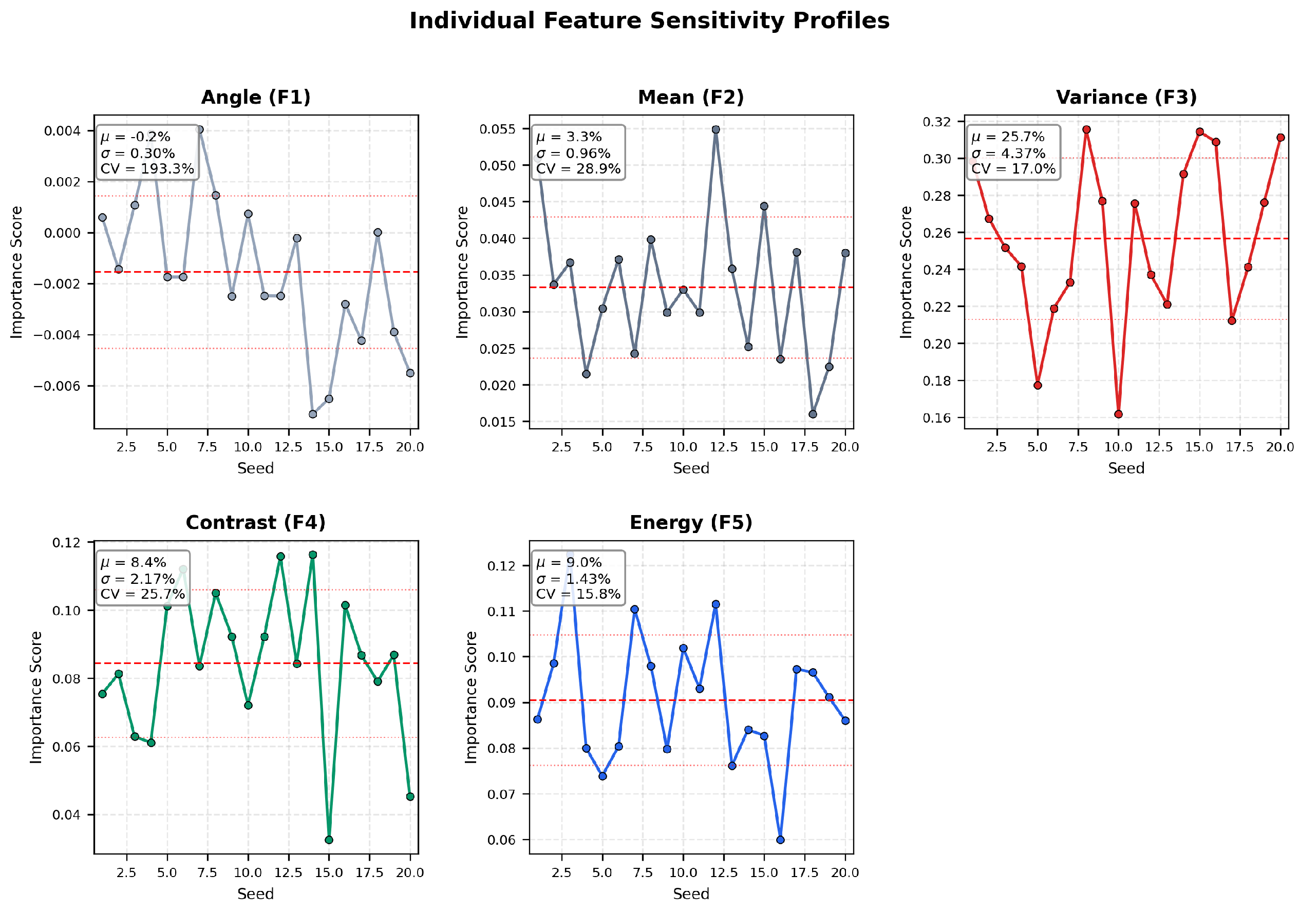
As illustrated in Figure 8, the sensitivity analysis of the input features highlights their differential contributions to the classification task, providing critical physical insights into the algorithm’s mechanics. Variance (F3) emerges as the most influential predictor, followed by Energy (F5) and Contrast (F4). This highlights that the structural blurring of light (high spatial variance dampening) is the most reliable physical proxy for cloud scattering, while the moderate importance of Energy (F5) suggests that textural uniformity—quantified by the GLCM angular second moment—also carries discriminative information under cloudy conditions, as cloud scattering reduces texture homogeneity in urban light networks. It is important to acknowledge that feature importance calculations in Random Forests (e.g., Gini importance) can sometimes be biased when input features are highly correlated, which is common among GLCM texture metrics. Despite this limitation, the overwhelming dominance of Variance remains physically consistent and is further substantiated by the robustness analysis shown in Figure 9.
The statistical dominance of Variance (F3) is deeply rooted in the physical scattering process of clouds. When upward-directed urban artificial lights penetrate a cloud layer, the water droplets and ice crystals induce intense multiple scattering. Physically, this transforms sharp, highly heterogeneous clear-sky light pixels into diffused and blurred halos. Mathematically, this structural blurring drastically dampens the high-frequency spatial variance within the GLCM. The second-ranked Energy feature (F5, 9.1%) captures the reduction in textural uniformity caused by cloud scattering—as clouds introduce spatial heterogeneity that disrupts the homogeneous light patterns of clear-sky urban networks. In comparison, the Angle feature (F1, 0.1 % ) plays a negligible role. Meanwhile, the Mean radiance (F2, 3.6%) provides only marginal information, which is physically sound, as the absolute brightness of city lights can easily fluctuate due to intra-night human activities (e.g., energy-saving dimming policies) or variations in satellite viewing geometry. Variance, being a relative metric of spatial heterogeneity, inherently filters out these macroscopic baseline shifts, serving as a highly robust and physically representative proxy for cloud-induced scattering.
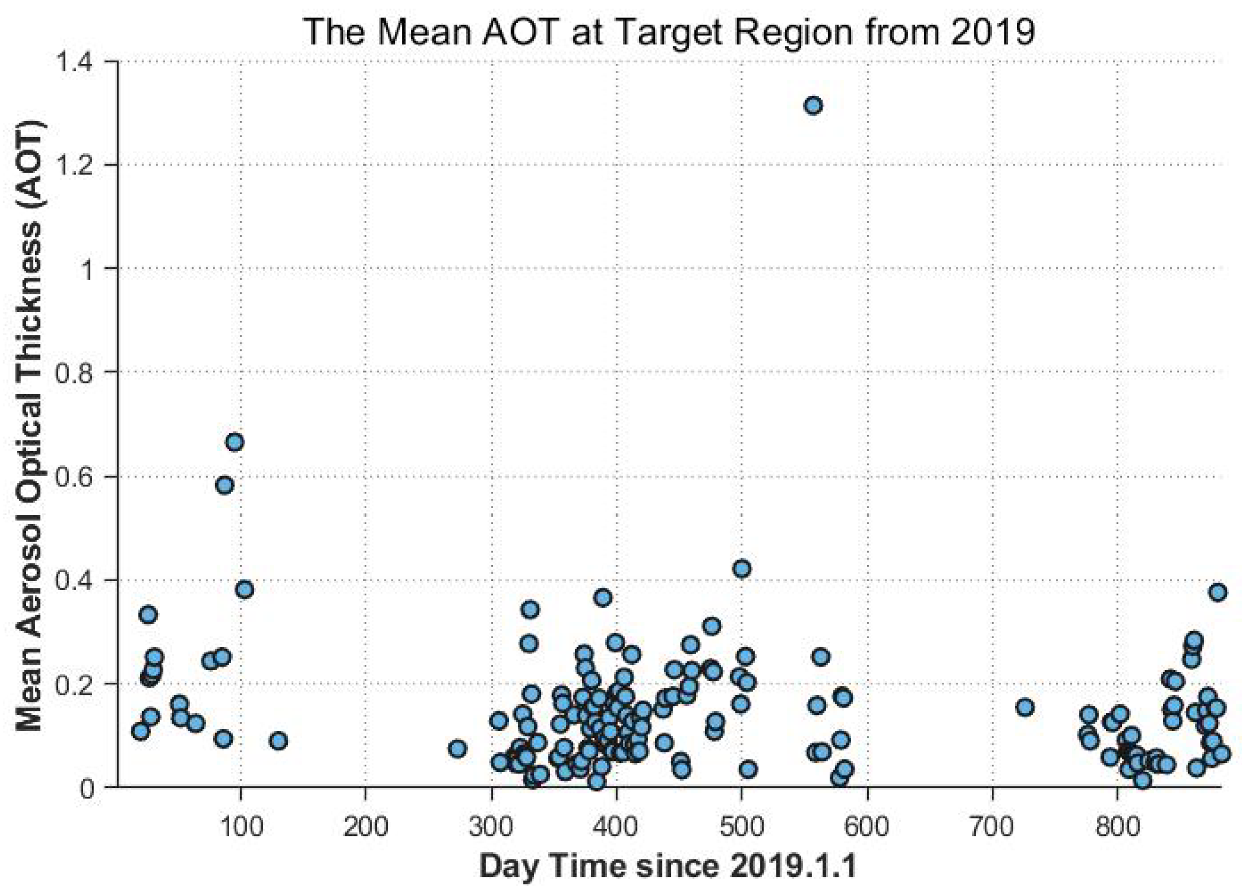
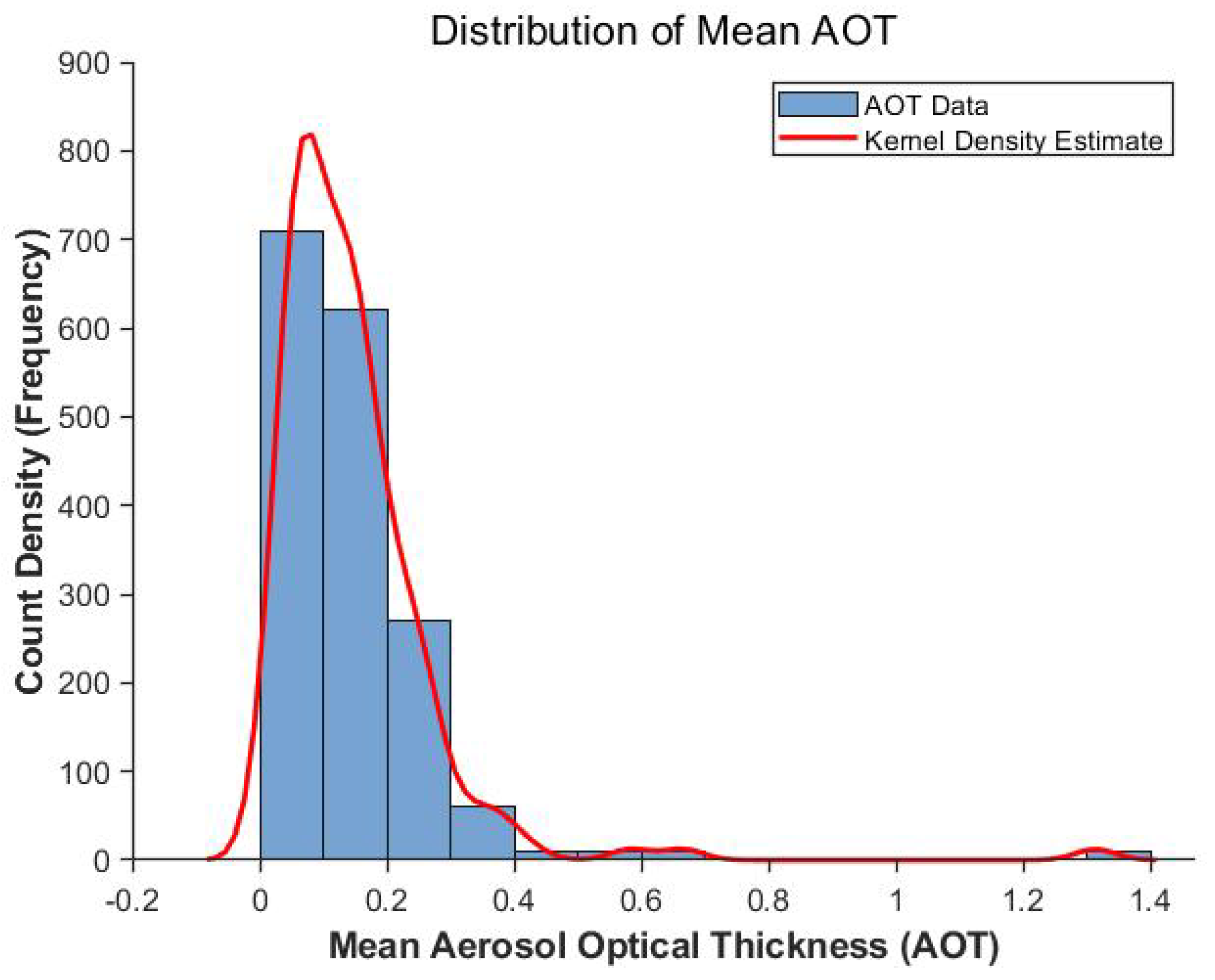
Regarding the influence of aerosols, as illustrated in the long-term time series Figure 10 and statistical distribution Figure 11, the target region exhibits a predominantly clean atmospheric background [28]. Quantitatively, the statistical analysis reveals that the vast majority of valid daytime AOD values over the experimental period remain strictly below a low optical threshold (e.g., AOD < 0.3 ). From a physical scattering perspective, such a low-concentration aerosol loading is optically insufficient to fully obscure the upward artificial light emissions. Consequently, the low-frequency scattering effect of these background aerosols acts primarily as a minor, constant radiance bias over a localized 20 × 20 observation window. This large-scale, low-magnitude aerosol blurring is effectively decoupled mathematically from the sharp, high-frequency textural variations induced by macroscopic cloud structures. Therefore, under these quantified clean atmospheric conditions, aerosol interference is safely mitigated by the spatial texture extraction process.

4.4. Performance Assessment Framework and Quantitative Evaluation

4.4.1. Evaluation Metrics and Experimental Protocol

To rigorously evaluate the generalization performance of the Random Forest model, we constructed a confusion matrix utilizing the independent ground-truth Ka-band radar dataset. The evaluation followed a strict protocol to ensure statistical independence: all 97 synchronized satellite-radar sample pairs were exclusively reserved as an external test set, with the model trained solely on the manually annotated data. Each sample pair represents a single VIIRS/DNB overpass temporally matched ( ± 5 min) with the co-located Ka-band radar profile, with a minimum 24-h separation between any two pairs to eliminate temporal autocorrelation. Among the 97 samples, 34 were labeled as Cloud and 63 as Clear by the radar ground truth (ratio approximately 1:1.9), indicating a moderate class imbalance toward clear-sky conditions. Based on the confusion matrix, four standard statistical evaluation metrics were calculated: Accuracy, Precision, Recall (Sensitivity), Specificity, and the F1-Score, as defined in Section 3.5.

4.4.2. Classification Performance

Table 3 presents the confusion matrix of the Random Forest model evaluated on the 97 independent test samples.
Based on this confusion matrix, the model achieved an overall accuracy of 86.6%. To rigorously assess statistical significance, a 95% Wilson score confidence interval was calculated, yielding [ 78.4 % ,   92.0 % ] . This interval is substantially above the chance-level accuracy of approximately 50% for a balanced two-class problem and above the majority-class baseline of 64.9% (i.e., always predicting the dominant Clear class). The model attained a precision of 80.0%, a recall (sensitivity) of 82.4%, a specificity of 88.9%, and an F1-score of 0.812. The high specificity indicates that the model successfully identifies clear-sky conditions, while the moderate recall reflects that the majority of cloud occurrences are captured. The false positives (FP = 7)—instances where the radar reports clear sky but the RF model detects texture features suggestive of cloud scattering—predominantly occur under two conditions: (1) optically thin aerosol layers that produce subtle low-frequency blurring without fully meeting the 20 dBZ radar detection threshold, and (2) highly tenuous cirrus clouds composed of small ice crystals that scatter sufficient upward light to perturb DNB texture but fall below the Ka-band radar’s sensitivity floor.

4.4.3. Feature Importance Analysis

The feature importance analysis (Figure 8) reveals Variance (F3) as the dominant predictor (25.8%), followed by Energy (F5, 9.1%), Contrast (F4, 8.5%), and Mean (F2, 3.6%). The Angle feature (F1) contributed negligibly ( 0.1 % ), indicating that absolute brightness carries minimal discriminative information for cloud detection—consistent with the physical expectation that cloud scattering affects spatial texture structure rather than overall radiance levels. The relatively high importance of Energy (F5) suggests that textural uniformity, disrupted by cloud-induced scattering, provides complementary discriminative information beyond simple variance. The feature-to-notation mapping is summarized in Table 4 for clarity.
This ranking is physically consistent: cloud-induced forward scattering acts as a spatial low-pass filter on urban light emissions, directly suppressing the high-frequency variance that characterizes sharp clear-sky cityscapes. The negligible importance of Angle (F1, 0.1 % ) confirms that dominant texture orientation provides minimal discriminative power, as cloud scattering affects all directions roughly equally in the GLCM averaging process. Meanwhile, the low importance of Mean radiance (F2, 3.6%) indicates than spatial texture structure for cloud discrimination, as uniform dimming from intra-night lighting changes does not disrupt the high-frequency spatial patterns targeted by the classifier. It is important to acknowledge that feature importance calculations in Random Forests (e.g., Gini importance) can exhibit bias when input features are highly correlated, which is common among GLCM texture metrics. Despite this limitation, the overwhelming dominance of Variance remains physically consistent and is further substantiated by the robustness analysis shown in Figure 9.

4.4.4. Comparison with VIIRS Cloud Mask

While the VCM is generally reliable, its nighttime performance is fundamentally limited by its dependence on thermal infrared channels. Validation studies of the MODIS cloud mask—the algorithmic predecessor of the VIIRS VCM—have documented a pronounced nighttime performance drop, from 87–90% during daytime to 68–71% at night [10]. Direct comparison with ground-based millimeter-wave radar further confirms that cloud mask products exhibit systematic omission errors over regions with low-altitude clouds and weak thermal contrast [29]. These limitations are not incidental but stem from the fundamental physics of TIR-based cloud detection at night: when solar heating of the surface is absent, the brightness temperature difference between low cloud tops and the underlying surface (ΔBT) collapses below the detection threshold of conventional split-window algorithms [11]. Advanced multi-channel TIR fusion schemes, such as the naive Bayesian approach of Heidinger et al. [30], partially mitigate this issue by incorporating probabilistic reasoning across multiple spectral tests, but the core limitation persists: at night, all passive optical cloud detection ultimately reduces to thermal emission contrast, which is intrinsically insufficient for low-level warm clouds.
In our test set, the traditional VCM method achieved only a 61.9% agreement with the Cloud Radar. To rigorously understand the physical drivers behind these VCM omissions, a retrospective analysis was conducted on the concurrent MWR vertical profiles for the misclassified data groups. The radar reflectivity profiles confirm that the vast majority of these VCM false negatives correspond to low-level cloud layers (e.g., stratocumulus with cloud tops generally distributed below 2 to 3 km). Because the traditional VCM algorithm heavily depends on multi-channel TIR brightness temperature differences to distinguish cold cloud tops from the warm ground, this lack of a significant thermal gradient renders the TIR channels largely blind to these low-level clouds.
In stark contrast, our single-channel texture-based model achieved an 86.6% agreement with the ground truth because it is entirely independent of thermal emissions, relying instead on the optical blurring of light. However, it is essential to interpret this comparative result through the lens of sensor-specific physics. The higher agreement of the RF model does not necessarily imply that the VCM is universally “wrong,” but rather reflects a fundamental divergence in the effective definitions of a “cloud.” The VCM defines night clouds primarily via top-down thermal emission deficits, whereas the Ka-band radar defines them via microwave backscatter from sufficiently large hydrometeors ( Z 20 dBZ). Because our RF model intrinsically relies on the physical forward-scattering of bottom-up artificial lights by similar hydrometeors, its effective definition of a cloudy pixel aligns much more closely with the radar’s physical perspective than with the TIR-based VCM, thereby yielding a higher statistical consensus in this specific application scenario.

5. Discussion

To rigorously evaluate the proposed algorithm and transparently address potential critiques, it is crucial to discuss the inherent limitations and applicability constraints of this methodology comprehensively.
A methodological question that warrants explicit discussion concerns the experimental design: specifically, whether integrating VCM, AOD, and Ka-band radar observations into a multi-source reference dataset would better support the study’s objectives. We address this as follows. The Ka-band millimeter-wave radar serves as the ground truth in this study because it provides the only physically independent, non-optical measurement of cloud presence at the study site. The VCM product, being derived from the same satellite platform using TIR algorithms, is not an independent reference—it is the very baseline against which we benchmark our method. Moreover, the VCM’s well-documented nighttime performance degradation [10,29], particularly its systematic failure to detect low-level warm clouds with minimal thermal contrast [11], means that incorporating VCM labels into the ground truth would propagate its TIR-specific omission errors into our evaluation, fundamentally undermining the independence of the validation. The daytime AOD product, while useful for characterizing the background aerosol environment, is a temporal proxy with inherent diurnal uncertainty and does not directly measure cloud presence. Combining these heterogeneous data sources into a single “reference” would conflate independent validation with correlated cross-comparison. We therefore maintain a clean experimental architecture: manual annotations train the RF classifier, and the independent Ka-band radar serves as the sole external validation standard. We acknowledge that multi-source data fusion for ground truth construction represents a valuable direction for future operational validation but falls outside the scope of the present preliminary feasibility demonstration.
First, a fundamental spatial mismatch exists between the ground-based radar and the satellite sensor. The millimeter-wave radar provides a point-source vertical profile (with a footprint of approximately 30 m), whereas the VIIRS/DNB pixel represents an area-source observation ( 750 m × 750 m ). Wind drift and the complex three-dimensional structure of broken clouds within this 750 m pixel can cause spatial representativeness errors, leading to inherent discrepancies between the exact overhead radar observation and the spatially averaged satellite signal.
Second, the stability of artificial ground lights is inevitably impacted by intra-night human activities. Satellite overpasses for SNPP occur around 01:30 a.m. local time (17:30 UTC), a period when many cities implement energy-saving policies, leading to the darkening or partial shutdown of urban lighting networks. However, because our Random Forest algorithm relies predominantly on high-frequency spatial texture features (e.g., Variance and Energy) rather than absolute radiance magnitudes, the uniform dimming of city lights acts primarily as a baseline scaling factor. It minimally disrupts the high-frequency structural blurring effects caused by clouds, thereby preserving the robustness of our texture-based approach.
Third, the algorithm’s effectiveness is strictly contingent upon the existence of ground-based artificial light sources. The borders of such artificially lit areas are inherently fuzzy and not easily defined from DNB images alone, as light intensity decreases gradually from urban cores to rural peripheries. In our evaluation framework, we define the operational area by the presence of detectable artificial light sources above the sensor noise floor within the 20 × 20 extraction window, as enforced by the radiance dynamic range quality threshold described in Section 3.3. However, the minimum light coverage fraction required for reliable performance—particularly at the urban-rural fringe where lit pixels occupy only a small fraction of the window—remains an open question for future multi-site investigation. Therefore, the method is primarily suited for artificially lit environments, such as urban and town areas, and cannot serve as a global solution over oceans, deserts, or unlit remote regions.
Fourth, it must be acknowledged that the current algorithm was validated under relatively clean atmospheric conditions (low Aerosol Optical Depth). While the model logically decouples the low-frequency scattering of moderate background aerosols from the high-frequency textures of clouds, its performance under high AOD or severe haze conditions remains untested. Extreme aerosol loading could severely attenuate the upward transmission of artificial light, drastically reducing the signal-to-noise ratio of the high-frequency cloud textures and potentially degrading detection accuracy. The robustness of this method in heavily polluted environments requires further investigation.
Fifth, the current algorithm is fundamentally a data-driven, empirical classifier. While the extracted high-frequency texture features successfully capture the macroscopic manifestations of cloud scattering, the model currently lacks explicit physical constraints derived from atmospheric radiative transfer (RT) theory. Incorporating rigorous RT constraints over artificially lit regions is extremely challenging, as it requires complex 3D radiative transfer modeling (e.g., Monte Carlo simulations) to properly couple the highly heterogeneous bottom-up urban light emissions with 3D cloud structures. Recent work by Sun et al. [23] has demonstrated the feasibility of such Monte Carlo-based 3D cloud radiance simulations for ground-based lighting scenarios, providing a promising pathway toward physically constrained models. Given the preliminary feasibility nature of this study, developing a physics-informed or hybrid physical–statistical model falls outside the current scope, but it remains a crucial theoretical limitation that must be addressed in subsequent algorithm iterations.
Sixth, regarding the potential interference from surface Bidirectional Reflectance Distribution Function (BRDF) and observation geometry, their impacts are inherently minimized by both the physical context and the algorithm design of this study. Surface BRDF primarily dictates the directional reflection of incident natural light. Because our methodology strictly enforces a zero-moonlight filter (Lunar Zenith Angle <90°), the observed DNB signals are overwhelmingly dominated by bottom-up artificial light emissions rather than top-down surface reflections, rendering BRDF effects virtually negligible. Furthermore, while variations in the satellite viewing zenith angle can alter the atmospheric path length and the absolute observed radiance, the VIIRS DNB utilizes a unique along-scan aggregation strategy that maintains a near-constant spatial resolution across the swath. Algorithmically, our reliance on localized ( 20 × 20 pixels) linear radiometric normalization (Equation (3)) prior to texture extraction dynamically offsets macroscopic, low-frequency baseline shifts caused by viewing geometry. Consequently, the relative high-frequency spatial structures of artificial lights, which serve as the primary features for the random forest model, remain highly robust against geometric variations.
To contextualize our results within the existing literature, a direct comparison with the most closely related prior work is instructive. Joachim and Storch [15] proposed a Random Forest classifier for nighttime cloud detection over urban areas using combined VNIR and VIIRS/DNB observations—the only prior study, to our knowledge, that applies machine learning to DNB-based cloud detection over cities. Their approach achieved an overall accuracy of approximately 70% under favorable lunar illumination conditions, but its performance is fundamentally constrained by the availability of moonlight, confirming the dependence on top-down natural reflectance. In contrast, our method deliberately operates exclusively under strictly moonless conditions, achieving 86.6% overall accuracy (95% CI: 78.4–92.0%) by relying solely on the bottom-up scattering of artificial lights. This comparison highlights the complementary nature of the two approaches: Joachim and Storch’s method performs optimally when moonlight is available, while our method fills the critical observational gap during moonless periods. Together, these two paradigms can provide continuous nighttime cloud monitoring capability across the full lunar cycle in artificially lit regions.
Our method also complements existing physical threshold-based nighttime detection approaches. Hu et al. [31] developed the Multi-channel Radiative Transfer Characteristics (MRTC) algorithm for nighttime fog and low stratus detection using VIIRS TIR channels, achieving a Probability of Detection of 0.86. While MRTC relies on multi-channel TIR brightness temperature differences optimized for specific cloud types, our single-channel DNB approach captures a fundamentally different physical signature—optical scattering rather than thermal emission—making it sensitive to cloud layers regardless of their thermal contrast with the surface. These two detection paradigms are therefore not competitive but synergistic, with each excelling under conditions where the other is physically limited.
Seventh, it is crucial to recognize that satellite-based cloud detection is fundamentally an application-dependent problem. Different detection algorithms establish different effective definitions of what constitutes a cloud based on their distinct underlying physical mechanisms. As noted previously, the Ka-band radar lacks sensitivity to extremely thin, high-altitude cirrus clouds with small ice crystals, whereas thermal infrared sensors might easily capture these cold tops but miss low-level warm clouds. Consequently, the proposed RF algorithm—which operates on the principle of optical texture blurring caused by hydrometeor scattering—establishes a detection threshold uniquely aligned with the disruption of ground light transmission. Therefore, the “cloud mask” generated by this method specifically represents clouds that are optically thick enough to scatter urban lights. This sensor-specific bias means our method should be interpreted not as an absolute, universal replacement for traditional cloud masks, but as a specialized, highly effective tool for defining and detecting cloud cover directly impacting optical visibility and radiation transfer over artificially lit regions.
Eighth, we must transparently acknowledge the limitations regarding the sample size. While the 97 rigorously synchronized data groups over 97 independent observation days provide a statistically significant foundation for evaluating local performance (as evidenced by the Wilson 95% CI of 78.4–92.0%), the dataset is relatively small compared to global operational satellite validation campaigns. Acquiring high-frequency, temporally matched, and zero-moonlight filtered ground-based millimeter-wave radar data is logistically challenging. Therefore, consistent with the title of this manuscript, the current results should be strictly interpreted as a “preliminary feasibility” study. Scaling this algorithm for operational use will absolutely require subsequent multi-site, multi-year evaluations encompassing much larger hold-out datasets to comprehensively capture regional climatological variances.
Ninth, the current validation is confined to a single geographic location (Longmen, subtropical monsoon climate) and a limited observation period (March to October 2020). The algorithm’s performance under winter conditions, in different climate zones (e.g., high-latitude cities with extended winter darkness, arid regions with distinct aerosol regimes), and across varying degrees of urbanization has not been assessed. The transferability of the trained Random Forest model to new cities without site-specific retraining also remains unexamined. These geographic and seasonal limitations must be acknowledged when interpreting the reported 86.6% accuracy, which should be understood as a site-specific feasibility demonstration rather than a globally validated performance claim.
Finally, regarding macro-geographic applicability, while urban and artificially lit areas constitute a small fraction (approximately 1% to 3%) of the global land surface, these regions are heavily populated and frequently suffer from complex aerosol pollution and urban heat island effects, making precise local cloud monitoring exceptionally critical. Therefore, rather than serving as a standalone global cloud mask, our method provides a highly valuable, localized complementary technique to existing TIR-based systems, specifically bridging the detection gap over complex urban environments under moonless conditions.

6. Conclusions

In this study, we demonstrated the feasibility of a novel approach for nighttime cloud detection under moonless conditions specifically tailored for artificially lit regions. Leveraging the unique scattering properties of ground artificial lights observed by the VIIRS/DNB sensor, we constructed a single-channel, texture-based classification algorithm utilizing a random forest model. When validated against the independent and highly reliable ground-based Ka-band Cloud Radar, the algorithm achieved an overall accuracy of 86.6% (95% CI: 78.4–92.0%) against millimeter-wave cloud radar observations on 97 independent test samples drawn from 97 observation days.
It is important to emphasize that the current findings represent the preliminary feasibility of a highly promising method. Moving forward, subsequent studies will extend this point-source validation framework to full satellite images, conducting larger-scale and longer-term comparative validations. By presenting this conceptual framework and methodology, we aim to inspire the broader scientific community to build upon this idea, ultimately driving the development of more accurate, robust, and widely applicable nighttime cloud detection algorithms.
This method strictly relies on the presence of stable artificial ground lights, making it primarily applicable to urban and artificially lit regions. Future research will focus on: (1) extending the methodology to moonlit conditions by developing radiometric normalization techniques to separate moonlight reflectance from artificial light scattering; (2) exploring the algorithm’s scalability in regions with sparser light networks (e.g., suburban or township areas) by establishing the minimum required light density thresholds; (3) expanding the research to observation stations across diverse climate zones, varying atmospheric pollution levels (including high-AOD conditions), and varying levels of urbanization to further validate and enhance the universal applicability of the model; and (4) developing physics-informed machine learning frameworks by integrating 3D atmospheric radiative transfer simulations of complex urban lights to provide rigorous physical constraints for the empirical texture features.

Author Contributions

Conceptualization, M.C. and S.H.; methodology, M.C.; software, M.C.; validation, M.C. and S.M.; resources, H.L.; writing—original draft preparation, M.C.; writing—review and editing, S.H. and S.M.; supervision, S.H. All authors have read and agreed to the published version of the manuscript.

Funding

This work was supported in part by the National Natural Science Foundation of China under Grant 42505139.

Data Availability Statement

The data presented in this study are available in accordance with the journal’s guidelines. The VIIRS/DNB satellite data are openly available from the NOAA Comprehensive Large Array-data Stewardship System (CLASS) (https://www.class.noaa.gov, accessed on 18 July 2024)). The ground-based millimeter-wave cloud radar data presented in this study are available on request from the corresponding author. The radar data are not publicly available due to privacy and institutional data-sharing policies.

Conflicts of Interest

The authors declare no conflicts of interest.

References

  1. Li, Z.; Shen, H.; Weng, Q.; Zhang, Y.; Dou, P.; Zhang, L. Cloud and Cloud Shadow Detection for Optical Satellite Imagery: Features, Algorithms, Validation, and Prospects. ISPRS J. Photogramm. Remote Sens. 2022, 188, 89–108. [Google Scholar] [CrossRef]
  2. Zhang, Y.C.; Rossow, W.B.; Lacis, A.A.; Oinas, V.; Mishchenko, M.I. Calculation of radiative fluxes from the surface to top of atmosphere based on ISCCP and other global data sets: Refinements of the radiative transfer model and the input data. J. Geophys. Res. Atmos. 2004, 109, D19105. [Google Scholar] [CrossRef]
  3. Gao, X.; Yang, J.; Xie, X.; Yang, Y.; Wang, N.; Cao, X.; Du, B.; Tan, M.; Xu, L.; Kou, Y. DG2-TCR: An Adaptive Clouds Removal Network for Optical Remote Sensing Images Using SAR-Driven Dual-Flow Fusion Guidance. IEEE Trans. Geosci. Remote Sens. 2025, 63, 5619016. [Google Scholar] [CrossRef]
  4. Irish, R.R.; Barker, J.L.; Goward, S.N.; Arvidson, T. Characterization of the Landsat-7 ETM+ Automated Cloud-Cover Assessment (ACCA) Algorithm. Photogramm. Eng. Remote Sens. 2006, 72, 1179–1188. [Google Scholar] [CrossRef]
  5. Zhu, Z.; Woodcock, C.E. Object-Based Cloud and Cloud Shadow Detection in Landsat Imagery. Remote Sens. Environ. 2012, 118, 83–94. [Google Scholar] [CrossRef]
  6. Li, Z.; Shen, H.; Li, H.; Xia, G.; Gamba, P.; Zhang, L. Multi-Feature Combined Cloud and Cloud Shadow Detection in GaoFen-1 Wide Field of View Imagery. Remote Sens. Environ. 2017, 191, 342–358. [Google Scholar] [CrossRef]
  7. Hagolle, O.; Huc, M.; Pascual, D.V.; Dedieu, G. A Multi-Temporal Method for Cloud Detection, Applied to FORMOSAT-2, VENµS, LANDSAT and SENTINEL-2 Images. Remote Sens. Environ. 2010, 114, 1747–1755. [Google Scholar] [CrossRef]
  8. Zhang, H.; Huang, Q.; Zhai, H.; Zhang, L. Multi-Temporal Cloud Detection Based on Robust PCA for Optical Remote Sensing Imagery. Comput. Electron. Agric. 2021, 188, 106342. [Google Scholar] [CrossRef]
  9. Qiu, S.; Zhu, Z.; He, B. Fmask 4.0: Improved Cloud and Cloud Shadow Detection in Landsats 4–8 and Sentinel-2 Imagery. Remote Sens. Environ. 2019, 231, 111205. [Google Scholar] [CrossRef]
  10. Kotarba, A.Z. A comparison of MODIS-derived cloud amount with visual surface observations. Atmos. Res. 2009, 92, 522–530. [Google Scholar] [CrossRef]
  11. Ackerman, S.; Frey, R.; Strabala, K.; Liu, Y.; Gumley, L.; Baum, B.; Menzel, P. Discriminating Clear-Sky from Cloud with MODIS Algorithm Theoretical Basis Document (MOD35); Technical Report; University of Wisconsin-Madison: Madison, WI, USA, 2010. [Google Scholar]
  12. Liao, L.B.; Weiss, S.; Mills, S.; Hauss, B. Suomi NPP VIIRS Day-night Band On-orbit Performance. J. Geophys. Res. Atmos. 2013, 118, 705–712, 718. [Google Scholar] [CrossRef]
  13. Kuciauskas, A.; Solbrig, J.; Lee, T.; Hawkins, J.; Miller, S.; Surratt, M.; Richardson, K.; Bankert, R.; Kent, J. Next-Generation Satellite Meteorology Technology Unveiled. Bull. Am. Meteorol. Soc. 2013, 94, 1824–1825. [Google Scholar] [CrossRef][Green Version]
  14. Cao, C.; De Luccia, F.J.; Xiong, X.; Wolfe, R.; Weng, F. Early On-Orbit Performance of the Visible Infrared Imaging Radiometer Suite Onboard the Suomi National Polar-Orbiting Partnership (S-NPP) Satellite. IEEE Trans. Geosci. Remote Sens. 2014, 52, 1142–1156. [Google Scholar] [CrossRef]
  15. Joachim, L.; Storch, T. Cloud detection for night-time panchromatic visible and near-infrared satellite imagery. ISPRS Ann. Photogramm. Remote Sens. Spat. Inf. Sci. 2020, 5, 853–860. [Google Scholar] [CrossRef]
  16. Vermote, E.; Justice, C.; Csiszar, I. Early Evaluation of the VIIRS Calibration, Cloud Mask and Surface Reflectance Earth Data Records. Remote Sens. Environ. 2014, 148, 134–145. [Google Scholar] [CrossRef]
  17. Li, Q.; Li, H.; Sun, X.; Ruan, Z.; Liu, L.; Gao, W.; Liao, C.; Ding, H. On the Quantification of Thermodynamic Phases of Raining Clouds: Insights From Multi-Year CloudSat and Ground-Based Radar Observations Over Longmen, Southern China. J. Geophys. Res. Atmos. 2025, 130, e2024JD041824. [Google Scholar] [CrossRef]
  18. Kollias, P.; Clothiaux, E.E.; Miller, M.A.; Albrecht, B.A.; Stephens, G.L.; Ackerman, T.P. Millimeter-Wavelength Radars: New Frontier in Atmospheric Cloud and Precipitation Research. Bull. Am. Meteorol. Soc. 2007, 88, 1608–1624. [Google Scholar] [CrossRef]
  19. Liu, L.; Zhang, Y.; Ding, H. Vertical Air Motion and Raindrop Size Distribution Retrieval Using a Ka/Ku Dual-Wavelength Cloud Radar and Its Preliminary Application. Atmos. Sci. 2021, 45, 1099–1113. [Google Scholar]
  20. Li, Y.; Sun, X.; Zhao, S.; Ji, W. Analysis of snowfall’s microphysical process from Doppler spectrum using Ka-band millimeter-wave cloud radar. J. Infrared Millim. Waves 2019, 38, 245–253. [Google Scholar]
  21. Guo, J.; Liu, H.; Wang, F.; Huang, J.; Xia, F.; Lou, M.; Wu, Y.; Jiang, J.H.; Xie, T.; Zhaxi, Y.; et al. Three-Dimensional Structure of Aerosol in China: A Perspective from Multi-Satellite Observations. Atmos. Res. 2016, 178–179, 580–589. [Google Scholar] [CrossRef]
  22. Frey, R.; Ackerman, S.; Holz, R.; Dutcher, S. The Continuity MODIS-VIIRS Cloud Mask (MVCM) User’s Guide; Technical Report; University of Wisconsin-Madison: Madison, WI, USA.
  23. Sun, H.; Hu, S.; Ai, W.; Ma, S. Monte Carlo Simulation of 3D Cloud Radiance Distributions Affected by Ground-Based Lighting. J. Geophys. Res. Atmos. 2026, 131, e2025JD045501. [Google Scholar] [CrossRef]
  24. Haralick, R.M.; Shanmugam, K.; Dinstein, I. Textural Features for Image Classification. IEEE Trans. Syst. Man Cybern. 1973, SMC-3, 610–621. [Google Scholar] [CrossRef]
  25. Johnson, R.S.; Zhang, J.; Hyer, E.J.; Miller, S.D.; Reid, J.S. Preliminary Investigations toward Nighttime Aerosol Optical Depth Retrievals from the VIIRS Day/Night Band. Atmos. Meas. Tech. Discuss. 2013, 6, 587–635. [Google Scholar] [CrossRef]
  26. Breiman, L. Random forests. Mach. Learn. 2001, 45, 5–32. [Google Scholar] [CrossRef]
  27. Belgiu, M.; Drăguţ, L. Random forest in remote sensing: A review of applications and future directions. ISPRS J. Photogramm. Remote Sens. 2016, 114, 24–31. [Google Scholar] [CrossRef]
  28. Holben, B.N.; Tanre, D.; Smirnov, A.; Eck, T.F.; Slutsker, I.; Abuhassan, N.; Newcomb, W.W.; Schafer, J.S.; Chatenet, B.; Lavenu, F.; et al. An emerging ground-based aerosol climatology: Aerosol optical depth from AERONET. J. Geophys. Res. Atmos. 2001, 106, 12067–12097. [Google Scholar] [CrossRef]
  29. Huo, J.; Han, C. Comparison of MODIS cloud mask products with ground-based millimeter-wave radar. Remote Sens. 2019, 11, 330. [Google Scholar] [CrossRef]
  30. Heidinger, A.K.; Pavolonis, M.J.; Holz, R.E.; Frey, R.A.; Ackerman, S. A naive Bayesian cloud-detection scheme derived from CALIPSO and applied within the VIIRS cloud mask. J. Appl. Meteorol. Climatol. 2012, 51, 1071–1089. [Google Scholar] [CrossRef]
  31. Hu, S.; Ma, S.; Yan, W.; Jiang, J.; Huang, Y. A New Multichannel Threshold Algorithm Based on Radiative Transfer Characteristics for Detecting Fog/Low Stratus Using Night-Time NPP/VIIRS Data. Int. J. Remote Sens. 2017, 38, 5919–5933. [Google Scholar] [CrossRef]
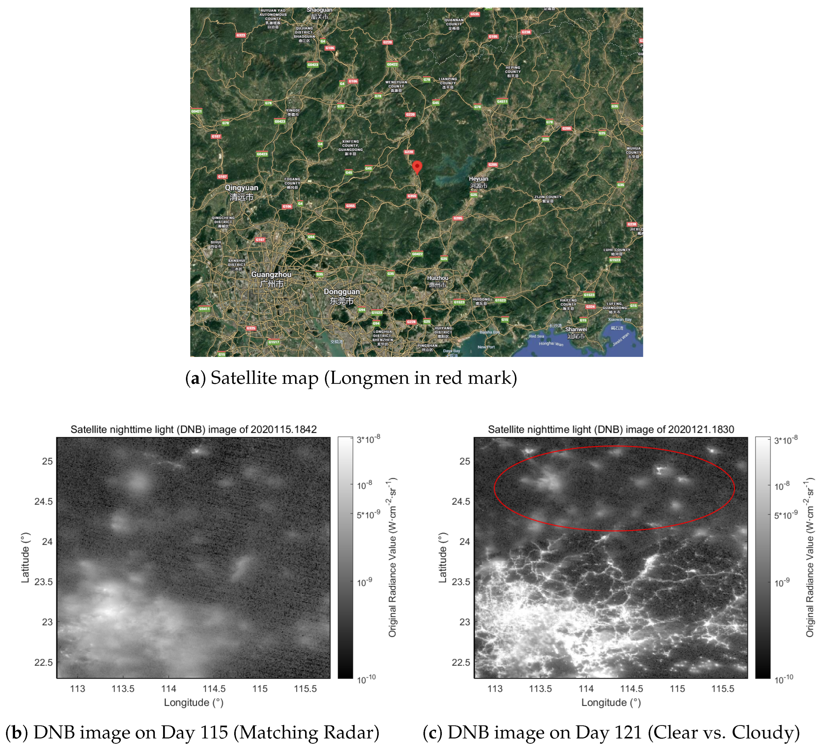
Figure 1. Study area and VIIRS/DNB nighttime light observations. (a) Satellite map showing the Longmen radar location; (b) DNB image at 18:42 UTC (02:42 a.m. local time) on Day 115 of 2020, temporally synchronized with the radar profile in Figure 2; (c) DNB image at 18:30 UTC (02:30 a.m. local time) on Day 121 of 2020, demonstrating the contrast between clear-sky city lights (bottom) and blurred lights under clouds (red circle).
Remotesensing 18 01956 g001
Figure 2. Profiles of radar reflectivity from the millimeter-wave cloud radar located in Longmen on Day 115 of the year 2020.
Remotesensing 18 01956 g002
Figure 3. Schematic diagram of the satellite descending orbit scanning mode.
Remotesensing 18 01956 g003
Figure 4. Flowchart of the training and operating process of the random forest model.
Remotesensing 18 01956 g004
Figure 5. Sensitivity analysis of the Random Forest model performance under different temporal matching windows ( ± 3 , ± 4 , ± 5 , and ± 6 min).
Remotesensing 18 01956 g005
Figure 6. Classification performance comparison using different DNB feature extraction window sizes: (a) 10 × 10 pixels, (b) 20 × 20 pixels, and (c) 30 × 30 pixels. In these matrices, “Predictor” denotes the Random Forest model output, and “Reference” denotes the ground-truth Radar observation.
Remotesensing 18 01956 g006
Figure 7. Nighttime Light Distribution in the Target Region Captured by VIIRS DNB at 18:12 on Day 23 of 2019.
Remotesensing 18 01956 g007
Figure 8. Sensitivity analysis of nighttime light data features of random forest model.
Remotesensing 18 01956 g008
Figure 9. Individual Feature Sensitivity Profiles.
Remotesensing 18 01956 g009
Figure 10. Mean Aerosol Optical Thickness in target region from 2019 to 2020.
Remotesensing 18 01956 g010
Figure 11. Time Series of Valid Mean AOT at Target Region.
Remotesensing 18 01956 g011
Table 1. Parameter Comparison of Multi-Source Datasets used in this Study.
Data ProductParameterChannel/FrequencySpatial Res.Temporal Res.
VIIRS DNBRadiance0.5–0.9 μm750 m6 min
Ka-band MWRReflectivity Factor (Z)33.44 GHz25 m vertical25–26 s
VCMCloud/ClearMulti-channel750 m6 min
VIIRS AOD L2Aerosol Optical ThicknessMulti-channel6 km6 min
Table 2. Data Screening Process and Rejection Criteria.
Screening StepReason for Rejection
Moonlight FilterLunar Zenith Angle <90° (Conservative geometrical filter to guarantee zero direct moonlight regardless of lunar phase)
Radar DowntimeMissing, corrupt, or uncalibrated ground truth data
Temporal MismatchNo valid VIIRS/DNB overpass within the matching window
Table 3. Confusion matrix of the Random Forest model evaluated on 97 independent test samples (Cloud = 34, Clear = 63). Values in parentheses are column-normalized percentages.
Radar: CloudRadar: Clear
RF: Cloud28 (82.4%)7 (11.1%)
RF: Clear6 (17.6%)56 (88.9%)
Table 4. Feature notation and description.
NotationFeature NamePhysical Interpretation
F1AngleOrientation of dominant texture patterns
F2Mean RadianceBaseline brightness of artificial lights
F3VarianceDispersion of pixel values; dampened by cloud scattering
F4ContrastIntensity of local spatial variations in GLCM
F5EnergyTextural uniformity (GLCM angular second moment)
Disclaimer/Publisher’s Note: The statements, opinions and data contained in all publications are solely those of the individual author(s) and contributor(s) and not of MDPI and/or the editor(s). MDPI and/or the editor(s) disclaim responsibility for any injury to people or property resulting from any ideas, methods, instructions or products referred to in the content.