Article

Energy-Efficient Spiking Spectral-Weighting Reconstruction Network for Compressive Hyperspectral Imaging


1
Key Laboratory of Photoelectronic Imaging Technology and System of Ministry of Education of China, School of Optics and Photonics, Beijing Institute of Technology, Beijing 100081, China
2
National Key Laboratory on Near-Surface Detection, Beijing 100072, China
*
Author to whom correspondence should be addressed.
Remote Sens. 2026, 18(11), 1805; https://doi.org/10.3390/rs18111805
Submission received: 13 March 2026 / Revised: 4 May 2026 / Accepted: 25 May 2026 / Published: 2 June 2026

Highlights

What are the main findings?
  • We overcome several major challenges in adapting spiking neural networks (SNNs) to compressive hyperspectral imaging (CHI) reconstruction tasks and propose the first SNN-based reconstruction network (SSWR-Net) to significantly improve the energy–efficiency ratio in CHI reconstruction.
  • Leveraging the proposed SNN-based spatial–spectral feature extraction modules, customized feature scaling architectures and a novel temporal-wise progressive training method, the proposed network, SSWR-Net, achieves energy-efficient and high-fidelity reconstruction performance on both simulation and real experiments.
What are the implications of the main findings?
  • The proposed network, SSWR-Net, overcomes the dependence of existing ANNs on high energy consumption and advanced hardware, making it possible to deploy CHI systems on energy-constrained devices.
  • The principles of this work are general, thus offering great potential to be generalized to various HSI-based classification and fusion tasks, as well as other inverse imaging problems.

Abstract

Recently, artificial neural networks (ANNs) have shown impressive performance in the compressive hyperspectral imaging (CHI) reconstruction task, but the high energy consumption limits their deployment on energy-constrained devices. This paper develops a novel spiking neural network (SNN), termed spiking spectral-weighting reconstruction network (SSWR-Net), to significantly improve the energy–efficiency ratio in CHI reconstruction. Firstly, a spiking spectral-weighting convolution block is proposed to adaptively modulate the spiking signals, enabling the SNN to fit continuous spectral correlation curves. Secondly, a residual feature reuse module with more direct connections is designed to achieve efficient and lightweight spatial–spectral feature extraction. Thirdly, customized feature scaling architectures are introduced to resolve the dimensional mismatch issue and enhance information flow. Finally, we propose a novel temporal-wise progressive training method to optimize the multi-timestep SSWR-Net, which can significantly improve both training efficiency and reconstruction quality. Both simulation and real experiments demonstrate the superiority of the proposed method in both CHI reconstruction performance and energy efficiency. Specifically, SSWR-Net outperforms its ANN-based counterpart by 0.87 dB at a 19.74% energy cost.

1. Introduction

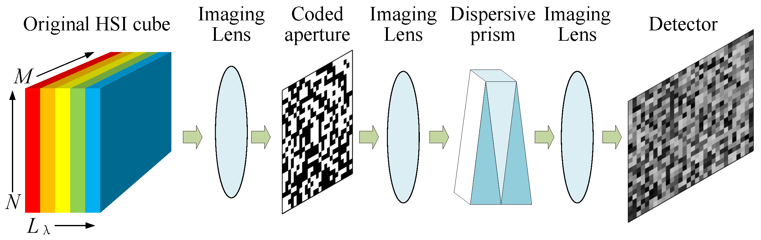
Hyperspectral images (HSIs) provide rich spectral and spatial information of the target scene, enabling diverse applications in material identification [1], environmental monitoring [2], forestry management [3] and other fields [4]. Conventional hyperspectral imaging systems based on spectral or spatial scanning architectures require a long data acquisition time, which limits their applications in dynamic imaging scenes [5,6,7]. To solve this problem, a novel compressive hyperspectral imaging (CHI) system, termed coded aperture snapshot spectral imager (CASSI) was proposed to effectively reduce imaging time and memory cost [7]. CASSI uses a two-dimensional (2D) coded aperture to modulate the three-dimensional (3D) HSI of the target scene. Then, different spectral bands are dispersed by a prism, and the modulated light field is finally projected on a focal plane array detector to generate 2D compressive measurements. Although CASSI is efficient for data acquisition, it requires intensive computing resources to inversely reconstruct the original 3D HSI from the compressive measurements.
Previously, lots of model-based methods and artificial neural networks (ANNs) were proposed to achieve high-fidelity and fast CHI reconstruction [8,9,10,11,12,13,14]. For example, state-of-the-art (SOTA) ANNs can reconstruct a CHI frame in less than 0.023 s with more than 37.50 dB. However, ANN-based methods rely heavily on high-energy-consumption advanced GPUs (NVIDIA GeForce RTX 4090 D), which require approximately 425 W to process a large number of high-precision data and perform high-energy-consumption multiply–add operations [13,14,15]. The development of energy-efficient CHI reconstruction methods is crucial to the practical deployment of CASSI on energy-constrained devices.
As the third generation of neural networks, brain-inspired spiking neural networks (SNNs) offer a spike-driven and energy-efficient computing paradigm [16,17,18]. They employ spiking neurons to perform sparse and low-energy accumulation operations, which are triggered only upon receiving discrete spiking inputs. Consequently, during the inference process, a large proportion of spiking neurons remain in the resting state, leading to negligible energy consumption. When implemented on tailored neuromorphic chips, including Loihi [19] and Tianjic [20], SNNs have been shown to achieve up to 1000 times higher energy efficiency than ANNs [20]. This intrinsic merit makes SNNs a promising candidate for energy-efficient and high-fidelity CHI reconstruction.
However, adapting SNNs to the CHI reconstruction task encounters several major challenges. Firstly, existing SNNs were mainly validated on simple classification tasks but lack validation on complex reconstruction tasks [21,22]. Secondly, the binary and discrete nature of spiking signals fundamentally limits their ability to express the continuous spectra in HSI data cubes [23]. Thirdly, efficient feature extraction and scaling architectures within SNNs remain underexplored [15]. Finally, the training of multi-timestep SNNs is often computationally expensive and yields sub-optimal performance [18,24].
To address these challenges, this paper proposes a novel SNN approach, termed spiking spectral-weighting network (SSWR-Net), to significantly improve the energy–efficiency ratio in CHI reconstruction while retaining preferred reconstruction fidelity. To the best of our knowledge, this is the first SNN-based paradigm for energy-efficient and high-fidelity CHI reconstruction. The contributions of this work are detailed in the following.
Firstly, SNN-based spiking spectral-weighting convolution (SSWC) is proposed to eliminate the mismatch between the binary spiking signals and the continuous spectra in HSIs. This block adopts trainable channel-wise weights and biases to adaptively modulate the binary spiking signals, thereby enhancing the representation ability of continuous spectra in HSIs while maintaining high-energy–efficiency spike-driven inference. Secondly, the SNN-based residual feature reuse (RFR) module is developed by integrating SSWC blocks with feature concatenation and element-wise redistribution operations, which serves as the basic unit of SSWR-Net. In contrast to vanilla residual blocks, the RFR module uses more direct connections to achieve efficient and lightweight spatial–spectral feature extraction. Thirdly, customized feature scaling modules are introduced to resolve the dimensional mismatch issue that limits the deployment of residual learning in SNNs. Specifically, the novel down-sampling and up-sampling architectures are designed to preserve necessary dimension transformations and to improve the information transmission capacity and reconstruction quality of the entire network. Finally, we propose a novel temporal-wise progressive training (TPT) method to efficiently optimize SSWR-Net. The TPT method leverages the implicit knowledge from previous timesteps to progressively fine-tune the parameters of the multi-timestep SSWR-Nets along the temporal dimension, which can significantly improve both training efficiency and reconstruction quality. Comprehensive experiments on both simulation and real datasets demonstrate the significant improvements of our method in both CHI reconstruction quality and energy efficiency over traditional ANN-based methods.

2. Related Works

2.1. CHI Reconstruction Methods

CHI reconstruction methods play a critical role in CASSI technology. Firstly, traditional model-based methods rely on various hand-crafted priors and iterative optimization algorithms to improve reconstruction quality [8,9]. Specifically, each iteration of these methods usually employs a data fidelity term and a prior term, aiming to alternately solve a data sub-problem and a prior sub-problem. For example, GAP-TV employed the generalized alternating projection (GAP) algorithm to solve a total variation minimization problem for each spectral band [8]. Although model-based methods typically enjoy mathematical interpretability, they are limited by sub-optimal reconstruction quality and long runtime.
With the advent of deep learning, several learning-based methods, including convolutional neural networks (CNNs) and Transformers, have been proposed for efficient CHI reconstruction [10,11,12]. Firstly, end-to-end methods have been proposed to directly learn the mapping function between the snapshot measurements and the original HSIs. For instance, λ -Net employs a generative adversarial network with a subsequent refinement stage to improve reconstruction quality [10]. TSA-Net integrates the spatial and spectral self-attention operations within a U-shaped CNN to decode deep features [11]. Moreover, end-to-end methods usually adopt a black-box design and lack interpretability.
Recently, deep unfolding methods have attracted considerable interest in CHI reconstruction, combining interpretability and generalization ability. Specifically, DU methods usually adopt iterative frameworks, utilizing a recovery module and a denoising module in each stage. GAP-Net incorporates U-shaped CNNs to perform the denoising step in the GAP method, thereby significantly improving reconstruction efficiency [14]. DGSMP adopts deep networks to simulate a sensing matrix and dynamically generates a gradient step in its recovery module [13]. DHUTNet introduces a U-shaped hybrid-attention Transformer in its denoising module to efficiently model various correlations of HSIs [25]. Although these ANN-based methods achieve superior reconstruction performance, their reliance on energy-intensive continuous computation and advanced hardware limits their deployment on edge computing devices.

2.2. SNN Training Method

Currently, there are two main strategies for implementing deep and high-performance SNNs, i.e., the ANN2SNN method and the direct training method. The ANN2SNN method firstly trains an ANN with rectified linear unit (ReLU) functions and preserves its network weights; then it replaces all ReLU functions in the pre-trained ANN with spiking neurons [26]. Thus, the converted SNN shares the architecture of the original ANN, aiming to approximate the activation values of artificial neurons (ReLU function) using the firing rates of spiking neurons. Although the ANN2SNN method achieves high accuracy, it requires long timesteps and does not fully leverage the event-driven nature of SNNs [21,22]. In contrast, the direct training method addresses the non-differentiability of binary spiking signals by employing the surrogate gradient (SG) within the backpropagation through time (BPTT) method, enabling the training of deep SNNs [24]. Compared with the ANN2SNN method, the direct training method requires fewer timesteps and provides more design flexibility to SNN architectures [18,21,24]. Therefore, this work adopts the direct training method to develop our SNN-based framework.

2.3. SNN Architecture

Effective network architectures are essential to addressing common challenges in directly training deep SNNs, including gradient vanishing/explosion and performance degradation [21]. Currently, various architectures with residual blocks have been adopted as fundamental components in SNNs [21,27]. For example, Spikingformer introduces a novel membrane shortcut to achieve identity mapping, while preserving spike-driven computation [28]. In terms of macro- and micro-architectures, Meta-SpikeFormer employs CNN-based residual blocks in its embedding part to enhance both performance and generalization ability [27]. Spike YOLO further shows that the complex ANN-based modules are often inefficient when directly applied to SNNs and that CNN-based architectures achieve superior performance compared with Transformer-based SNNs [22]. Furthermore, Spike YOLO achieved accuracy comparable to that of ANN-based DETR at the cost of 17.49% computational energy consumption in the object detection task. This efficiency gain was mainly attributed to the fact that Spike YOLO only uses energy-efficient sparse addition operations, and the number of its operations is lower than the energy-intensive multiply– addition operations in DETR. Moreover, to address the representational limitation of binary spiking signals, PA-EVSNN employs membrane potential (MP) neurons for event-based video reconstruction [23]. MP neurons consume more energy but provide richer and continuous spatio-temporal information within the SNN-based encoder and decoder. Within the field of HSIs, SNNs are predominantly applied to classification tasks [15]. But the potential of SNNs for the more challenging reconstruction task remains unexplored. To the best of our knowledge, this work presents the first systematic investigation on the feasibility of SNNs for achieving energy-efficient and high-fidelity CHI reconstruction.

3. Preliminaries

In this section, we introduce the mathematical model of the CASSI system and the neuronal dynamics of spiking neurons.

3.1. The Mathematical Model of the CASSI System

Figure 1 shows the schematic of the CASSI system, which encodes the 3D spectral–spatial information of a target scene into 2D compressive measurements. Let G R N × M × L λ be the original HSI cube of the target scene, where N, M and L λ represent the height, width and the number of spectral bands, respectively. The forward imaging model of CASSI can be expressed as follows.
Firstly, G is spatially modulated by a 2D coded aperture C R N × M , which can be formulated as
G 1 ( n , m , l λ ) = G ( n , m , l λ ) C ,
where ⊙ represents the element-wise product; G 1 R N × M × L λ is the encoded HSI cube; n = 1 , , N and m = 1 , , M denote the horizontal and vertical spatial coordinates; and l λ = 1 , , L λ denotes the spectral slice. Then, a prism is used to shift each spectral slice of G 1 along the dispersive direction. The shifted HSI cube is defined as G 2 R N × M s × L λ , where M s = M + α · ( L λ 1 ) and α is the dispersion rate of the prism. Specifically, this dispersion process can be described as
G 2 [ n , m + α · ( l λ 1 ) , l λ ] = G 1 ( n , m , l λ ) .
Finally, a 2D monochromatic detector captures G 2 and generates the 2D compressive measurement Y R N × M s , which is formulated as
Y = l λ = 1 L λ G 2 ( : , : , l λ ) + O ,
where O R N × M s represents the additive sensing noise on the detector. Furthermore, Equation (3) can be rewritten in the following matrix form:
y = A g + o ,
where A R N M s × N M L λ is the sensing matrix of CASSI, including the contributions of the coded aperture and dispersive prism, and y , g and o represent the vectorized forms of Y , G and O , respectively [29].
Benefiting from its elaborate optical structure, the CASSI system can capture the 3D spectral–spatial information of the target scene in a single snapshot. But a challenging problem is how to recover the original HSI G from the compressive measurement accurately and efficiently. For a transmissive CASSI system, the detector and the computing device are the primary sources of energy consumption. Specifically, the detector (Basler acA2040-90μm, Beijing, China) consumes approximately 5 W, while the edge computing device (NVIDIA Jetson AGX Orin, Santa Clara, CA, USA) used for running ANNs consumes at least 75 W. Consequently, the computing device accounts for the majority of the total power consumption, approximately 93.75%. Moreover, if we want to develop ANNs with higher reconstruction accuracy and inference speed, it is usually necessary to employ higher-power GPUs. Therefore, an energy-efficient and high-fidelity reconstruction method is crucial to the practical deployment of CASSI on energy-constrained devices.

3.2. A Brief Review of Spiking Neurons

In contrast to the energy-intensive continuous computation of artificial neurons, spiking neurons perform energy-efficient and spike-driven computations [16]. Similarly, spiking neurons transmit information by leveraging discrete binary spikes across both spatial and temporal dimensions.

3.2.1. The Leaky Integrate-and-Fire Neuron

The leaky integrate-and-fire (LIF) neuron is the most widely used spiking neuron in SNNs [30]. The LIF neuron simplifies the computational model while preserving three crucial characteristics, including the leaking, integrating and firing operations. Next, the dynamics of the LIF neuron at timestep t are described.
First, the LIF neuron integrates input spiking signals from the presynaptic neurons and updates its MP as follows:
M ˜ t l , j = ( 1 1 τ ) M t 1 l , j + 1 τ i W l i j I t l 1 , i
where M ˜ t l , j denotes the MP of the j t h LIF neuron in the l t h neural layer before the firing operation; M t 1 l , j is the MP of the same neuron after the firing operation at timestep t 1 ; I t l 1 , i represents the emitted spiking signal from the i t h presynaptic neuron of the ( l 1 ) t h neural layer; W l i j is the synaptic weight; and the constant τ is the MP decay rate across timesteps.
Equation (5) models the leaking and integrating processes of the LIF neuron. The first and the second terms in Equation (5) represent the contributions of the previous state (temporal information) and the current input, respectively. Then, the firing process of the LIF neuron can be described as follows:
s t l , j = H ( M ˜ t l , j M t h ) ,
where H ( · ) is the Heaviside step function and M t h is the firing threshold. If MP M ˜ t l , j exceeds M t h , the LIF neuron will release a spiking signal ( s t l , j = 1 ) to its postsynaptic neuron; otherwise, it remains in the resting state ( s t l , j = 0 ).
Then, after the firing operation, the MP of the LIF neuron is reset to M t l , j . Taking the hard reset method as an example, if s t l , j = 1 , then M t l , j = 0 ; otherwise M t l , j = M ˜ t l , j .

3.2.2. Membrane Potential Neuron

Based on the LIF neuron, we introduce the dynamics of the MP neuron [23]. Different from the binary spiking signals of the LIF neuron, the MP neuron can output its MP during the firing process, which can be expressed as
s t l , j = M ˜ t l , j , M ˜ t l , j M t h 0 , o t h e r w i s e .
Moreover, the leaking and integrating operations of MP neurons are the same as those of LIF neurons. According to Ref. [23], MP neurons lead to less information loss than LIF neurons and can approximate continuous values in natural images more accurately. These characteristics are crucial to improving the reconstruction quality within a few timesteps.

4. Proposed Method

In existing SNNs, the static image is typically adopted as the input at each timestep. In this section, we introduce the details of our network structure and training method under the single-timestep inference paradigm.

4.1. The Overall Framework of the Spiking Spectral-Weighting Network

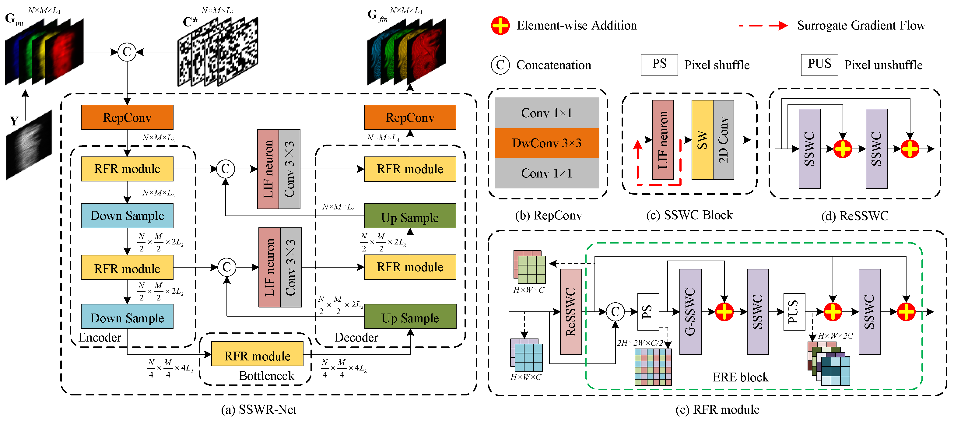
As illustrated in Figure 2, the input of the proposed network, SSWR-Net, consists of a 2D measurement Y and C * R N × M × L λ . C * R N × M × L λ is constructed by repeating C for L λ times along the spectral dimension. Firstly, following Ref. [12], we process Y to acquire the initial reconstruction result G i n i R N × M × L λ , which is defined as
G i n i ( n , m , l λ ) = Y ( n , m + α · l λ ) ,
Secondly, the concatenation of G i n i and C * is fed into the initial embedding module of SSWR-Net to encode the input data and produce the low-level feature F l R N × M × L λ [23,31]. This process can be written as
F l = R e p C o n v [ c a t ( G i n i , C * ) ] = F 1 × 1 c o n v { F 3 × 3 D c o n v { F 1 × 1 c o n v [ c a t ( G i n i , C * ) ] } } ,
where R e p C o n v ( · ) is the mapping function of the embedding module, as shown in Figure 2b; F 1 × 1 c o n v ( · ) represents a convolutional function with kernel size 1 × 1 ; and F 3 × 3 D c o n v ( · ) represents a depth-wise convolutional function with kernel size 3 × 3 . Thirdly, F l propagates through the SNN-based backbone for T timesteps to generate the deep feature F d , which is obtained by averaging the outputs of the final layer in the backbone over all T timesteps.
Finally, F d is decoded by a mapping module to produce the final reconstruction result G f i n . In this paper, SSWR-Net with T timesteps is denoted SSWR-Net-T.

4.2. SNN-Based Backbone

As shown in Figure 2a, our SNN-based backbone employs the typical three-level U-shaped architecture, including an encoder, a bottleneck and a decoder.

4.2.1. Spiking Spectral-Weighting Convolution Module

There is a fundamental mismatch between the inherent binary nature of spiking signals and the continuous spectra in HSI data cubes, which is critical in HSI-based tasks. To bridge this gap, we propose an SNN-based SSWC block to efficiently model these correlations.
As shown in Figure 2c, the SSWC block comprises an LIF neuron, a spectral-weighting (SW) function and a convolutional layer connected in sequence. During the training process, the SW function adaptively assigns channel-wise floating-point spectral weights and biases to the binary spiking tensor emitted from the LIF neuron. Specifically, given an input P f R H × W × C , the computation of the SSWC block can be described as follows:
O w = S S W C ( P f ) = F k s × k s c o n v { S W [ L I F ( P f ) ] } = F k s × k s c o n v [ k · L I F ( P f ) + b ] ,
where S S W C ( · ) , L I F ( · ) and S W ( · ) represent the mapping functions of the SSWC block, LIF neuron and SW function, respectively; k R C and b R C are the learnable floating-point weights and bias parameters of S W ( · ) , respectively. Thus, during the forward process, the floating-point data from the SW function enables the subsequent convolutional layer to perform efficient multiply accumulation operations. Meanwhile, during the backward propagation process, the learnable k and b introduce additional channel-wise gradients, which enable the network to fit the continuous spectra.
After training, we employ the reparameterization method to integrate k and b of S W ( · ) into the subsequent convolutional layer, which can be described as follows: Specifically, following the standard formulation of the 2D convolutional layer, we denote the patch in P f corresponding to the ( i , j , u ) th position of O w by P f i j R k s × k s × C , and p f i j R k s 2 · C × 1 is the vectorized form of P f i j . For the uth filter in the convolutional layer of Equation (10), let W o w u R 1 × k s 2 · C and b o w u R 1 × 1 be the vectorized forms of the weight and bias. Then, we construct Kr R k s 2 · C and Br R k s 2 · C by repeating k and b k s 2 times, respectively. Consequently, the ( i , j , u ) th position of O w is given by:
O w i , j = W o w u · ( Kr p f i j + Br ) + b o w u = ( W o w u Kr ) · p f i j + W o w u · B r T + b o w u .
The right part of Equation (11) represents the formulation of a 2D convolutional layer. Thus, the weight and bias of the uth filter in the convolutional layer of Equation (10) can be updated as:
W ¯ o w u = W o w u Kr , b ¯ o w u = W o w u · B r T + b o w u .
Thus, during inference, the SSWC block becomes a spike-driven module without sacrificing its representational ability.

4.2.2. Residual Feature Reuse Module

Although ANNs and SNNs can share identical topological structures, directly implementing complex ANN-based modules in their SNN counterparts often leads to the spike degradation problem [22,27]. Meanwhile, feature reuse approaches are widely adopted in ANNs to improve their generalization performance [32]. However, their effectiveness within SNNs remains underexplored.
Motivated by these findings, a simple but efficient SNN-based RFR module is proposed by integrating SSWC blocks with feature concatenation and element-wise redistribution operations, which serves as the basic unit in our SSWR-Net. It also employs membrane shortcuts to alleviate the gradient vanishing/explosion problems of SNNs. In contrast to vanilla SNN-based residual blocks, the proposed RFR module uses more direct connections to achieve efficient and lightweight spatial–spectral feature extraction. Its computational process is described as follows.
Given an input P i R H × W × C , the RFR module first employs a residual SSWC (ReSSWC) block to generate an initial feature O r s R H × W × C . As shown in Figure 2d, the ReSSWC block includes two SSWC blocks and two membrane shortcuts, which can be expressed as
O r s = R e S S W C ( P i ) = S S W C [ S S W C ( P i ) + P i ] + P i ,
where R e S S W C ( · ) denotes the function of the ReSSWC block. To further refine O r s , we propose a lightweight element-rearrangement-enhancement (ERE) block, which is shown in the green box of Figure 2e.
For a single 2D convolutional layer with a fixed kernel size in SNNs, a fewer number of input and output channels can effectively reduce the number of operations, thereby reducing its energy consumption. Thus, based on this principle, we adopt the pixel shuffle (PS) operation to reduce the parameters in the ERE module, which further reduces the energy consumption of SSWR-Net. First, a PS operation is applied to the concatenation of P i and O r s . This operation rearranges the elements of the concatenated feature to generate a feature map O p s R 2 H × 2 W × C / 2 with higher spatial resolution. In addition, the PS operation reduces the number of channels (from 2 C to C / 2 ), thereby decreasing the parameters for the subsequent SSWC block. Subsequently, O p s is processed by two SSWC blocks and then restored to the resolution of O r s through a pixel unshuffle (PUS) operation. This process is formulated as
O p s = P S ( c a t [ O r s , P i ] ) O e = P U S { S S W C [ G S S W C ( O p s ) + O p s ] } + O r s ,
where P S ( · ) and P U S ( · ) represent the PS and PUS operations, respectively, and G S S W C ( · ) represents the SSWC block using the group convolutional layer. The element redistribution processes of the PS and PUS operations are visualized in Figure 2e. Finally, a residual component is produced by processing O e with an SSWC block. The final output O r f r R H × W × C of RFR block is:
O r f r = S S W C ( O e ) + O r s .
Moreover, to address the high channel dimension at the bottleneck, the PS and PUS operations are integrated into the last SSWC block of the RFR module. Thus, Equation (15) is modified for the bottleneck layer as follows:
O r f r = P U S { S S W C [ P S ( O e ) ] } + O r s .
In this work, the kernel size of all SSWC blocks within the RFR module is set to 5. Moreover, we employ a single RFR module at each level of the SNN-based backbone to achieve efficient and lightweight spatial–spectral feature extraction.

4.2.3. Customized Feature Scaling Modules

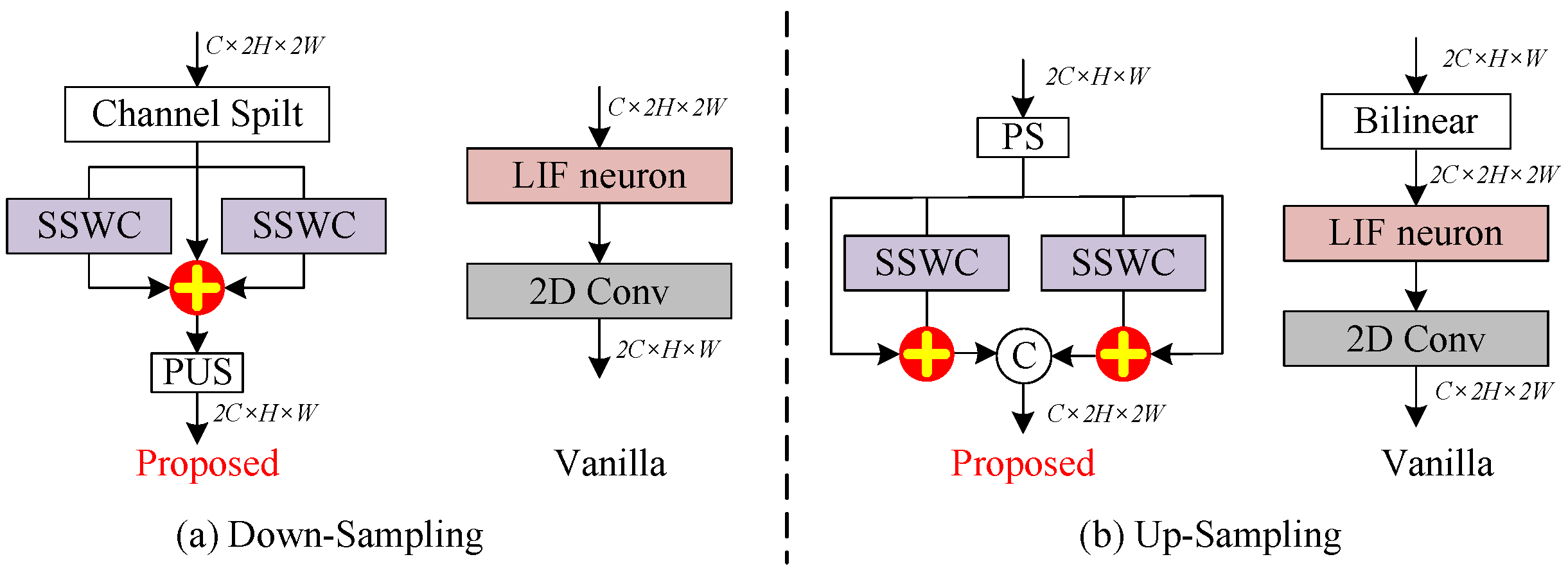
Feature scaling modules are essential components for dimension transformation in the U-shaped backbone [10,11,23]. As shown in the right parts of Figure 3a,b, the vanilla down-sampling module in SNNs typically consists of an LIF neuron followed by a 3 × 3 convolutional layer with a stride of 2. The vanilla up-sampling module in SNNs sequentially performs a bilinear interpolation step, an LIF neuron and a 3 × 3 convolutional layer. Previous works indicate that membrane shortcuts can significantly improve both the accuracy and training stability of SNNs. Furthermore, residual connections mitigate the gradient vanishing problem and suppress excessively low firing rates in SNNs. Although the lower firing rates reduce energy consumption, they also constrain the representational capacity of SNNs. However, the dimensional mismatch between the input and output features prevents the direct application of identity connection in the vanilla feature scaling modules.
To address this issue, we propose customized down-/up-sampling modules (as shown in the left parts of Figure 3a,b) that integrate the SSWC blocks with membrane shortcuts. They overcome the dimensional mismatch issue that limits the deployment of residual learning in SNNs. Specifically, for a given input E d i n R C × 2 H × 2 W , our customized down-sampling module first splits E d i n along the channel dimension into two sub-tensors, i.e., e d i n , 1 R C / 2 × 2 H × 2 W and e d i n , 2 R C / 2 × 2 H × 2 W . Then, the sub-tensor is processed by an independent SSWC block with a membrane shortcut. This process is formulated as
e d , 1 o u t = S S W C d 1 ( e d , 1 i n ) + e d , 1 i n , e d , 2 o u t = S S W C d 2 ( e d , 2 i n ) + e d , 2 i n ,
where S S W C d 1 ( · ) and S S W C d 2 ( · ) represent the two SSWC blocks used in the proposed down-sampling module. Finally, e d o u t , 1 and e d o u t , 2 are fused, and the resulting feature is resized to produce the final output E d o u t R 2 C × H × W . This process is formulated as:
E d o u t = P U S ( e d , 1 o u t + e d , 2 o u t ) .
In addition, given an input E u i n R 2 C × H × W , our customized up-sampling module first employs the PS function to obtain e u i n R C / 2 × H / 2 × W / 2 . Then, e u is processed by two independent SSWC blocks with membrane the shortcuts, which can be formulated as
e u o u t , 1 = S S W C u 1 ( e u i n ) + e u i n , e u o u t , 2 = S S W C u 2 ( e u i n ) + e u i n ,
where S S W C u 1 ( · ) and S S W C u 2 ( · ) represent the two SSWC blocks used in our up-sampling module. Finally, e u o u t , 1 and e u o u t , 2 are concatenated along the channel dimension to obtain the final output E u o u t R C × 2 H × 2 W . That is,
E d o u t = c a t ( e u , 1 o u t , e u , 2 o u t ) .
The customized architectures successfully integrate the membrane shortcuts into the feature scaling modules, preserving necessary dimension transformations. Furthermore, the proposed down-/up-sampling modules enable efficient gradient propagation and improve the reconstruction quality of SSWR-Net. The kernel size of all SSWC blocks within our down-/up-sampling modules is set to 3.

4.3. Temporal-Wise Progressive Learning Method

Efficient learning methods for SNNs have attracted considerable research interest [21]. Currently, most SNNs rely on the conventional BPTT method with SG to overcome the non-differentiability of LIF neurons when optimizing the parameters. However, the BPTT method introduces two fundamental challenges, including the high computational burden caused by temporal unfolding and the accumulation of quantization errors caused by the binary spikes [21,24]. These limitations lead to high training cost and usually result in sub-optimal performance for multi-timestep SNNs. Given the temporal dynamics of SNNs, the implicit knowledge encoded within a pre-trained short-timestep SSWR-Net provides a valuable prior to facilitate the training of multi-timestep SSWR-Net.
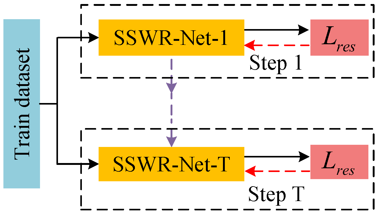
Inspired by these findings, we propose a novel TPT method to leverage the implicit knowledge from previous timesteps to progressively optimize the network parameters along the temporal dimension. Taking SSWR-Net-4 as an example, Figure 4 illustrates the workflow of the proposed TPT method. Specifically, the purple arrows indicate the flow of network parameters, and the red arrows indicate the backpropagation path of the surrogate gradients. The TPT method operates as follows.
Step 1: We first initialize SSWR-Net-1 with random weights. Then, all parameters in SSWR-Net-1 are optimized for 250 epochs using the BPTT method with SG. The reconstruction loss function is defined as
L r e c = R M S E ( G , G f i n ) ,
where R M S E ( · ) is the root mean square error (RMSE) function; G and G f i n represent the ground-truth and the reconstructed HSI, respectively. In this training process, we employ the Adam optimizer ( b e t a 1 = 0.9 and b e t a 2 = 0.99 ) with a learning rate of 2 × 10 3 . The batch size is 5, and each epoch includes 2000 training samples.
Step 2: SSWR-Net-2 is initialized by inheriting the architecture and parameters from the well-trained SSWR-Net-1, while the number of timesteps is set to 2. This provides a sub-optimal starting point for the subsequent fine-tuning process. The initialized SSWR-Net-2 is then fine-tuned for 80 epochs using the Adam optimizer and the Cosine Annealing scheduler with a learning rate of 2 × 10 4 .
Step 3: Similarly, we extend the timesteps of the well-trained SSWR-Net-2 to 3 and initialize SSWR-Net-3 with a sub-optimal starting state. Then, by using the same training settings in Step 2 but halving the number of epochs, SSWR-Net-3 is fine-tuned for 40 epochs to obtain a well-trained SSWR-Net-3.
Step 4: Finally, we extend the timesteps of the well-trained SSWR-Net-3 to 4 and initialize SSWR-Net-4 with a sub-optimal starting state. Then, using the same training settings in Step 2 but halving the number of epochs, SSWR-Net-4 is fine-tuned for 20 epochs to obtain a well-trained SSWR-Net-4.
For a multi-timestep SSWR-Net, our TPT method can significantly reduce the training epochs by transferring prior knowledge along the temporal dimension and improve reconstruction quality.

5. Experiments

This section compares the proposed network, SSWR-Net, with several SOTA methods on both simulation and real datasets. Furthermore, various ablation experiments are conducted to verify the contribution of each proposed module.

5.1. Experimental Settings

5.1.1. Datasets

In the simulations, we utilize three publicly available HSI datasets, namely, CAVE [33], KAIST [34] and ARAD_1K [35]. Following the settings of previous works, we employ the CAVE dataset for training and select ten scenes from the KAIST dataset for testing. However, the CAVE and KAIST datasets comprise only indoor scenes. In contrast, the ARAD_1K dataset includes various outdoor real-world scenes. To evaluate the generalization ability of each learning-based model in different environments, we augment the test dataset with ten scenes from the ARAD_1K dataset.
The real experiments employed two real-world datasets. The first dataset comprises the compressive measurements of five scenes, which were real-captured by Ref. [11] and are widely used in CHI reconstruction works. The real CASSI system in Ref. [11] captured 28 spectral bands ranging from 450 nm to 650 nm with a 10 nm interval, and each spectral band is of size 660 × 660 . Moreover, the shifting step α of its prism is 2 (based on the system structure). Thus, according to Equation (4), the spatial size of compressive measurement for each scene is 660 × 714 . However, the first dataset lacks the original HSIs, preventing the quantitative assessment of reconstruction results. To overcome this limitation, we built up another CASSI testbed to obtain the second real dataset, which includes several pairs of original HSIs and compressive measurements used for training and testing. The reconstruction results on the second real dataset can quantitatively demonstrate the effectiveness of the proposed method. The experimental settings and reconstruction results on our testbed are provided in Section 5.3.

5.1.2. Implementation Details

In the simulation experiments, similar to Refs. [11,13,36], the HSI cubes from those public datasets are interpolated into 28 spectral channels, ranging from 450 nm to 650 nm, and the shifting step α of the prism is set to 2. The original HSIs and corresponding compressive measurements are of size 256 × 256 × 28 and 256 × 310 for the simulations. For hardware configurations, this work uses an NVIDIA RTX 4090 D GPU (Santa Clara, CA, USA), an Intel Core Ultra 7 265K CPU (Santa Clara, CA, USA) and 64 GB of memory. All learning-based models are implemented using Python 3.10 and PyTorch 2.6.0. All spiking neurons are implemented using the SpikingJelly framework. During the training process, the data augmentation operations used include the random cropping of the 3D patches followed by random flipping and rotation.

5.1.3. Competing Methods

As is widely recognized in the field of SNNs, SNNs are primarily designed to improve the energy–efficiency ratio of artificial intelligence applications, but they intrinsically involve an accuracy trade-off compared with ANNs. Consequently, existing SNN-based methods typically treat their ANN-based counterparts and several representative ANNs as competing methods in the evaluation of energy consumption. We follow this widely accepted practice to ensure a fair and robust evaluation. We compare our SSWR-Net with several existing CHI reconstruction methods, including two model-based methods (GAP-TV [8] and TwIST [9]) and five ANN-based methods ( λ -Net [10], TSA-Net [11], DGSMP [13], GAP-Net [37] and SSWNet-A). These learning-based competing methods are implemented according to the settings reported in their original papers. Specifically, SSWR-Net-A is the ANN counterpart of the proposed network, SSWR-Net, in which all spiking neurons are replaced with ReLU functions. For a fair comparison, each learning-based model is trained using the same number of data samples per epoch and the same data augmentation methods. Moreover, to the best of our knowledge, our SSWR-Net is the first work to systematically explore the feasibility of using SNNs for CHI reconstruction. Thus, in this paper, we also conduct extensive ablation studies to demonstrate the contribution of proposed methods to the field of SNNs. Specifically, we compare the proposed methods against the widely used down-/up-sampling techniques in SNNs, and the feature extraction modules introduced in SOTA SNN-based methods.

5.1.4. Evaluation Metrics

We evaluate the performance of each competing method from three perspectives: (1) reconstruction accuracy, measured by the peak signal-to-noise ratio (PSNR) and structure similarity index measure (SSIM); (2) model complexity, represented by the number of parameters (Params); (3) energy cost, estimated by the total energy consumption in millijoules (mJ) [27]. These metrics enable a comprehensive and quantitative comparison. Generally, higher PSNR and SSIM indicate better reconstruction quality, while lower Params and energy consumption are preferred.
Specifically, consistent with existing SNNs, this paper adopts a standard theoretical estimation method to calculate the computational energy consumption for each learning-based method. This estimation method provides the energy consumption of various 32-bit floating-point operations based on 45 nm technology. In this case, the energy consumption for a single multiply operation and a single accumulate operation is denoted by E M U = 3.7 pJ and E A C = 0.9 pJ, respectively. For each learning-based method, let N M U and N A C represent the total number of multiply and accumulate operations, respectively. For a convolutional layer connected to an artificial neuron, the number of multiply operations ( N M U C o n v , a ) and that of accumulate operations ( N A C C o n v , a ) during the inference process are given by
N M U C o n v , a = N A C , a C o n v = k s 2 · H · W · c i n · c o u t ,
where k s is the kernel size of the convolutional layer, c i n and c o u t are the number of input and output channels, and H and W are the height and width of the output feature map. For a convolutional layer connected to an LIF neuron, the total number of multiply operations ( N M U C o n v , s ) and that of accumulate operations ( N A C C o n v , s ) are given by
N M U C o n v , s = 0 , N A C C o n v , s = t = 1 T F R t · k s 2 · H · W · c i n · c o u t ,
where T is the total number of timesteps for this LIF neuron and F R t is the firing rate of this LIF neuron at timestep t, representing the ratio of spiking elements in its emitted spiking tensor. Furthermore, the MP neuron shares the same energy consumption estimation method as the artificial neuron. Consequently, the total number of multiply and accumulate operations of each learning-based method during the inference process can be defined as N M U and N A C , respectively. Thus, the total energy consumption of each learning-based method is calculated as E t o t a l = N M U · E M U + N A C · E A C .

5.2. Results of Simulation Experiments

Table 1 presents the quantitative results of each competing method on the 10 test scenes from the KAIST dataset. In addition to SSWR-Net, we report the results of SSWR-Net*, which is an enhanced version of SSWR-Net. Specifically, SSWR-Net* first employs two RFR modules in each stage (encoder, bottleneck and decoder) of its SNN-based backbone, then replaces the two LIF neurons in the skip connection between the encoder and decoder with the MP neurons. SSWR-Net*-3 is also trained with the proposed TPT method. Although increasing the numbers of timesteps and RFR modules can further improve the reconstruction quality, it also increases the energy consumption. Consistently with existing directly trained SNNs, we employ a maximum of four timesteps and conduct systematic experiments to evaluate the effects of different timesteps and network depth on reconstruction quality and energy consumption.
The results in Table 1 show that compared with all baseline methods, our method achieves optimal or sub-optimal reconstruction quality on most of the test scenes with significantly lower energy consumption. Specifically, our SSWR-Net-1 outperforms λ -Net by 2.85 dB at a 1.48% energy cost (8.01 mJ/542.71 mJ) and matches the reconstruction quality of TSA-Net at a 1.58% energy cost (8.01 mJ/506.28 mJ). Our SSWR-Net*-3 outperforms DGSMP and GAP-Net by 0.50 dB and 0.45 dB at 23.16% energy cost (73.84 mJ/318.83 mJ) and 2.48% energy cost (73.84 mJ/2974.59 mJ), respectively. Compared with DGSMP and GAP-Net, our SSWR-Net and SSWR-Net* require considerably fewer parameters. Moreover, we adjust the network depth of DGSMP and GAP-Net used in Table 1 to obtain their lightweight versions, which have a similar number of parameters to that of our SSWR-Net*. The PSNR, Param and energy costs of the lightweight versions of DGSMP and GAP-Net are 30.90 dB/2.49 M/1694.69 mJ and 32.82 dB/2.85 M/212.55 mJ, respectively. It can be observed that compared with the lightweight versions of DGSMP and GAP-Net, SSWR-Net*-3 demonstrates a significant advantage in both reconstruction quality and energy efficiency. These results demonstrate the advantages of the proposed method in achieving lightweight feature extraction. Obviously, the energy consumption of the ANN-based models is significantly higher than that of the SNN-based models, severely limiting their deployment on energy-constrained devices.
Moreover, our SSWR-Net-1 and SSWR-Net-4 outperform SSWR-Net-A by 0.05 dB and 0.87 dB at 6.77% energy cost (8.01 mJ/118.29 mJ) and 19.74% energy cost (23.35 mJ/118.29 mJ), respectively. In addition, SSWR-Net-4 achieves a 0.82 dB higher PSNR than SSWR-Net-1, which is a significant improvement for CHI reconstruction. The performance of most directly trained SNNs is often inferior compared with their ANN-based counterparts in fewer timesteps. However, our SSWR-Net outperforms SSWR-Net-A within just one timestep. This is primarily because the structure of SSWR-Net is designed to fully exploit the core characteristics of spiking neurons.
Furthermore, we evaluate the generalization capability of the seven learning-based models on 15 test samples selected from the ARAD_1K dataset. Table 2 lists the average PSNR and SSIM results for each model. We emphasize that for this experiment, each pre-trained model obtained in Table 1 is directly applied without any fine-tuning on the ARAD_1K dataset. Thus, the Params and energy cost of each method are consistent with those reported in Table 1. Although each model shows some performance degradation, SSWR-Net* maintains superior performance, achieving optimal or sub-optimal results.
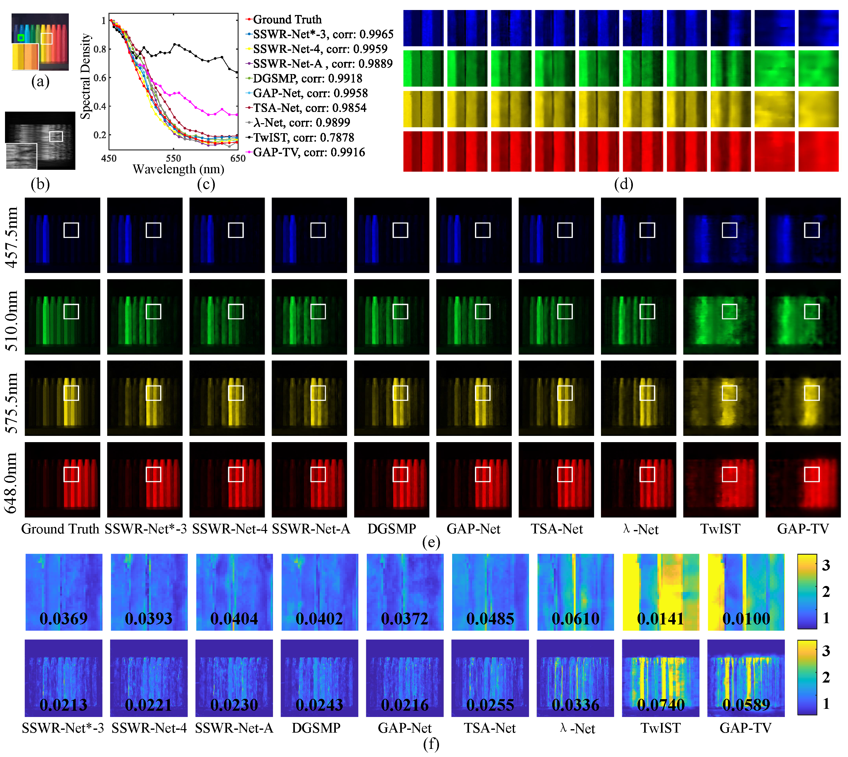
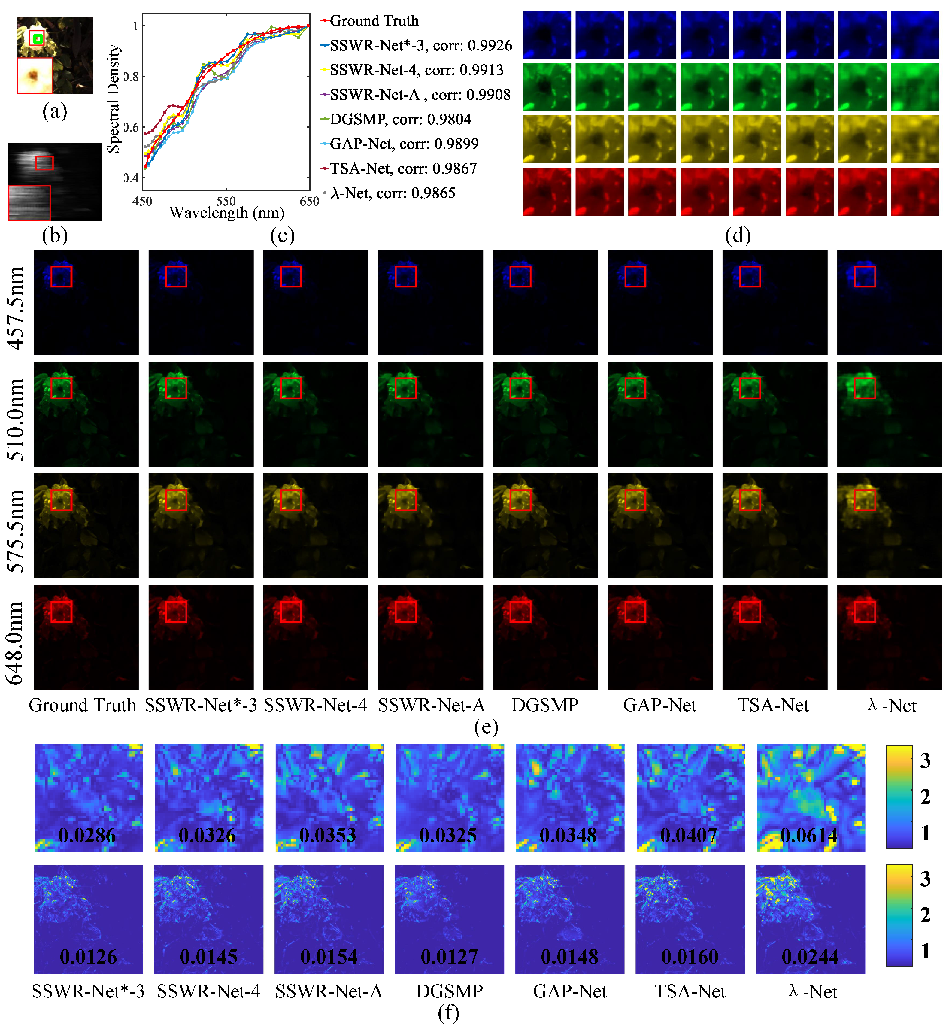
To evaluate visual reconstruction quality, we select one representative test scene each from the KAIST and ARAD_1K datasets. Figure 5 shows the reconstruction results on “Scene 9” of the KAIST dataset. It shows the images of four spectral channels selected from the HSIs. This scene contains rich spatial and spectral information. The RGB image and the corresponding compressive measurement of this scene are presented in Figure 5a and Figure 5b, respectively. Figure 5d shows the magnified images of the regions marked by white boxes in the reconstructed HSIs (shown in Figure 5e). SSWR-Net*-3 preserves more edge information and fewer artifacts while maintaining spatial smoothness. In addition, Figure 5c presents the spectral density curves of all reconstruction results and the reference curve (corresponding to the green box in the RGB image). The spectral correlation coefficient between each reconstructed curve and the reference curve is also provided. Our SSWR-Net*-3 achieves the highest correlation, demonstrating its exceptional spectral fidelity.
Furthermore, we provide the residual error map for each reconstruction image, offering an intuitive visualization of the reconstruction errors, particularly in texture regions. The residual error maps of the magnified patches/reconstructed HSIs are shown in Figure 5f. Specifically, we first calculate the absolute value of the 3D residual error data cube between each 3D magnified patch/reconstructed HSI and its reference image. Then, the 3D residual error data cubes are summed along the spectral axis to generate the final 2D residual error maps. Compared with the uniform background regions, the texture regions tend to exhibit larger reconstruction errors. The RMSE values of all magnified patches/reconstructed HSIs are provided at the bottom of each sub-figure. It shows that the proposed method achieves the lowest RMSE.
Following the layout of Figure 5, Figure 6 presents the visual performance of all methods on “Scene 3” of the ARAD_1K dataset. Consistently with the results in Figure 5, our method also achieves the best visual performance, including spatial and spectral fidelity. These results collectively demonstrate the superior reconstruction performance of the proposed method.

5.3. Results of Real Experiments

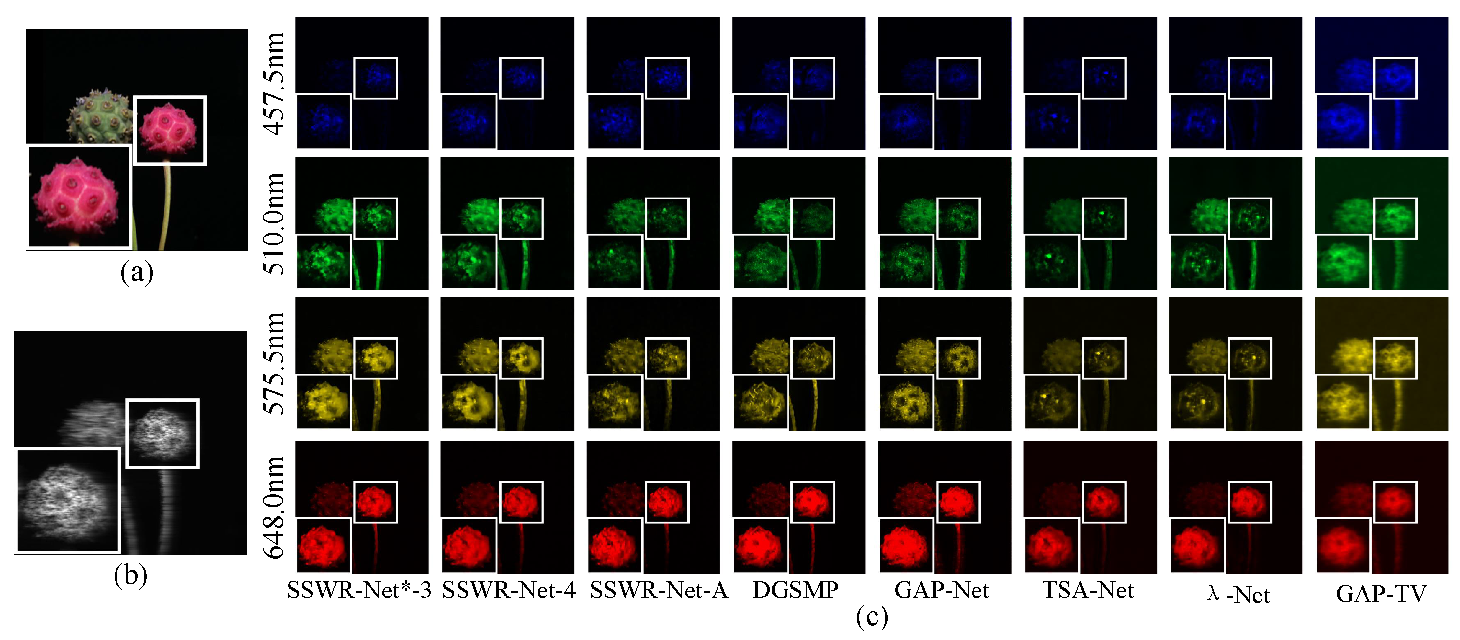
This section comprehensively evaluates the proposed method on two real datasets, as described in Section 5.1.1. For the first dataset, following the same training settings in Refs. [11,14], each learning-based competing method is re-trained on the CAVE and KAIST datasets. Figure 7 presents the reconstruction results of the proposed method and several representative competing methods using “Scene 4” in the first dataset. Figure 7a and Figure 7b present the RGB image and the compressive measurement of the target scene, respectively. Figure 7c shows 4 out of 28 spectral bands of the reconstructed HSIs. For each reconstructed image, the region marked by the white box is magnified. Compared with all competing methods, the proposed method preserves more detailed textures and more complete background information with fewer visual artifacts.
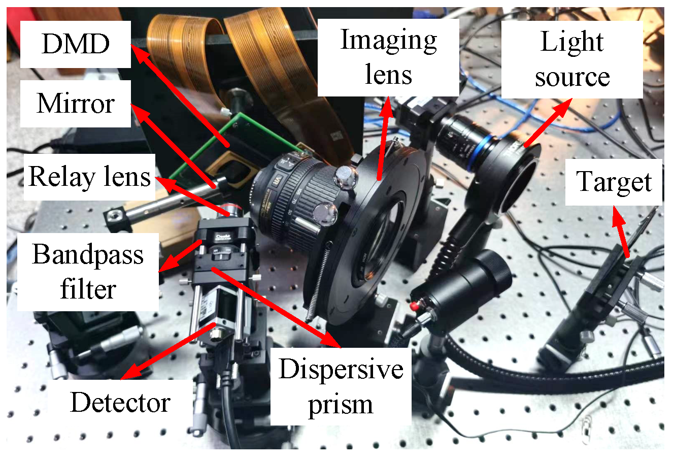
As mentioned in Section 5.1.1, the first real dataset lacks the original HSIs. Thus, we built a CASSI testbed to establish the second real dataset, including the original HSIs of target scenes. The detailed information of our testbed was described in Ref. [38]. Our CASSI system can capture nine spectral bands, ranging from 556 nm to 644 nm. The spatial size of the original HSIs is 256 × 256 , and the shifting step α is 1. Thus, the spatial size of the compressive measurements is 256 × 264 . A picture of our CASSI testbed is shown in Figure 8.
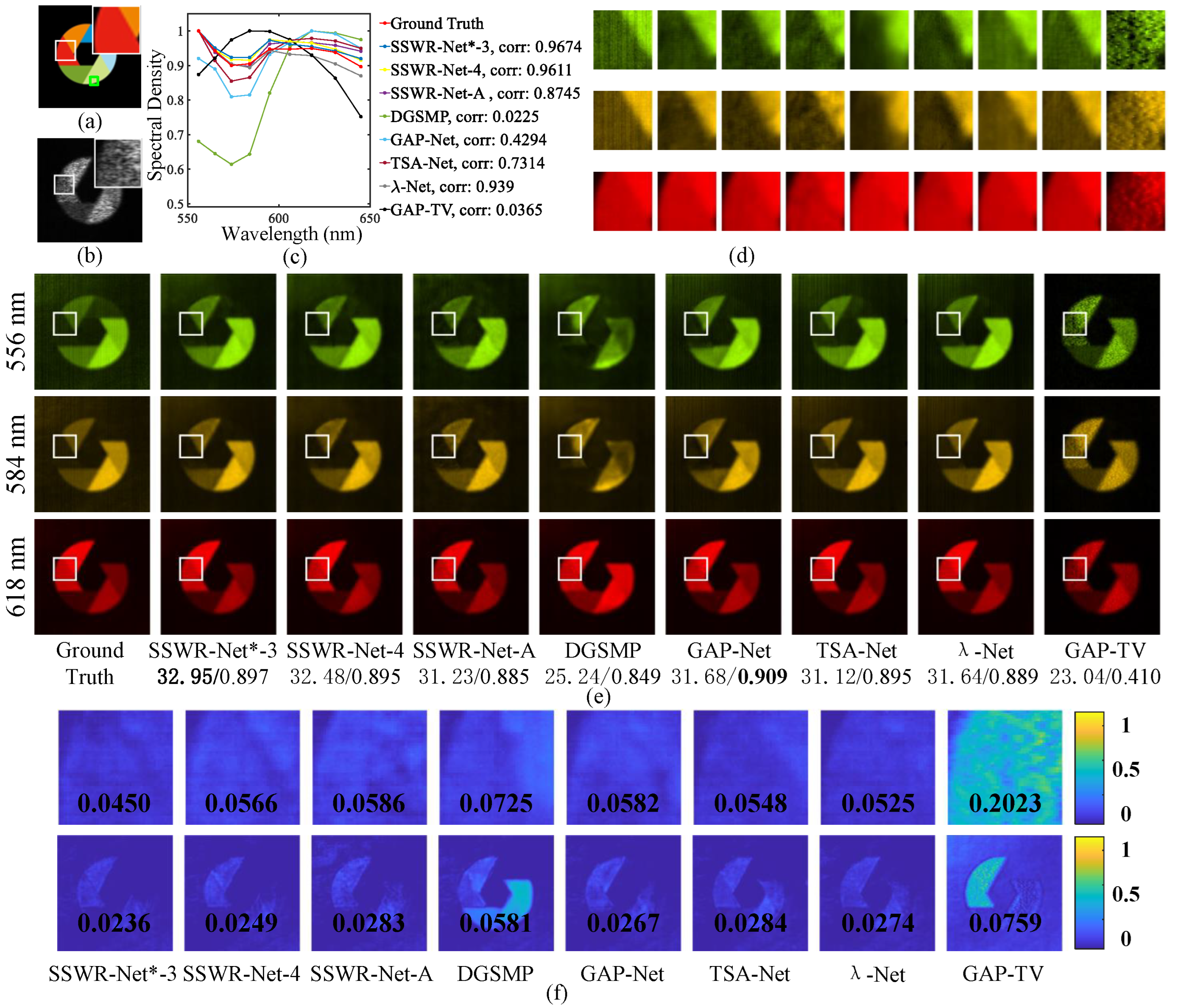
In the experiment on the second real dataset, the channel dimensions of both input and output layers in all learning-based methods are set to nine to ensure a fair comparison. Using the training settings in Table 1, all learning-based competing methods are pre-trained with the CAVE dataset. For our CASSI testbed, the signal-to-noise ratio between the real measurements and the simulated measurements is close to 10 dB. Thus, 10 dB Gaussian white noise (which is o in Equation (4)) is injected into the simulated measurements during the pre-training process. Then, following the experimental setting in Ref. [39], the training and test datasets are collected using our CASSI testbed to fine-tune and evaluate each learning-based model. Figure 9 presents three reconstructed spectral bands of “Scene 5” in the second real dataset. Moreover, the PSNR and SSIM values for each reconstructed image are provided in Figure 9e. Compared with the other competing methods, SSWR-Net*-3 and SSWR-Net-4 achieve superior reconstruction accuracy and better spectral correlation coefficients. These results demonstrate the advantages of the proposed method in terms of visual quality, spectral precision and spatial fidelity on the real CASSI system.

5.4. Ablation Study

This section performs ablation studies to verify the contribution of each proposed component in our SSWR-Net. The used test samples are selected from the KAIST dataset.

5.4.1. Break-Down Ablation on RFR Module

The ablation study on the proposed RFR module is conducted using baseline-1. Baseline-1 is derived by removing both the S W ( · ) function and the PS/PUS (element redistribution) operations from the RFR module in SSWR-Net-1. The results are shown in Table 3, where baseline-1 yields 31.56 dB PSNR, 0.890 SSIM, and 7.49 mJ energy cost. When we add S W ( · ) , the model yields a 0.59 dB improvement in PSNR but consumes an additional 4.14 mJ of energy. When we add the PS/PUS operations, the model yields negligible improvement in reconstruction quality but significantly reduces Params and energy cost. In addition, when we adopt both S W ( · ) and the PS/PUS operations, the model achieves a 0.59 dB improvement in PSNR while consuming only an additional 0.52 mJ and fewer Params. Moreover, compared with baseline-1 using S W ( · ) , our SSWR-Net-1 achieves a comparable PSNR at the cost of 52.40% Params and 68.87% energy. Due to this reduction in Params, the model exhibits a slight decrease in the SSIM. However, considering the significant efficiency gains in terms of Params and energy cost achieved by the PS/PUS operations, this slight decline is acceptable.

5.4.2. Ablation Study on Customized Feature Scaling Module

In this section, another ablation experiment is conducted for the customized feature scaling modules. This experiment uses baseline-2, which is obtained by replacing our customized down-/up-sampling modules with vanilla down-/up-sampling modules in SSWR-Net-1. The vanilla down-/up-sampling techniques are widely used in existing SNNs. The results are shown in Table 4. Baseline-2 yields 30.09 dB PSNR and 0.839 SSIM. When we adopt the customized down-sampling module or the customized up-sampling module in baseline-2, the reconstruction PSNR is improved by 0.29 dB and 1.31 dB, respectively. When both customized feature scaling modules are jointly used, the model achieves a 2.06 dB improvement in PSNR. The lowest energy consumption of baseline-2 mainly comes from the inefficient information transmission of its vanilla feature scaling modules. This suppresses the firing rate of spiking neurons, and consequently reduces the reconstruction quality of the entire model.

5.4.3. Comparison of Different Feature Extract Modules

We present an additional experiment to demonstrate the effectiveness of the proposed RFR module. We compare the RFR module with three existing SNN-based feature extract blocks, including two kinds of CNN-based blocks (SNN-CNN-1 [27] and SNN-CNN-2 [22]) and one Transformer-based block (SNN-Trans-1 [27]) introduced in recent SOTA SNN-based methods. Specifically, the RFR module in SSWR-Net-1 is replaced with these comparative blocks separately, and the results are shown in Table 5. It is observed that our RFR module outperforms the comparative modules in both reconstruction accuracy and energy cost. SNN-CNN-1 and SNN-CNN-2 achieve comparable reconstruction quality with our RFR module, but they have significant limitations in Params and energy cost. That is, our RFR module reduces the energy cost by 1.06 mJ and 0.57 mJ at the cost of 39.22% and 38.07% Params, respectively. Moreover, although the Transformer-based feature extraction block achieves impressive performance in ANNs, it shows significant limitations in SNN-based CHI reconstruction. In particular, although SNN-Trans-1 consumes fewer Params, it has a significant gap in reconstruction quality compared with the CNN-based blocks. The proposed RFR module outperforms SNN-Trans-1 by 2.37 dB at a 81.63% energy cost. This demonstrates the advantage of the RFR module in lightweight spatial–spectral feature extraction.

5.4.4. Ablation Study on TPT Method

Finally, we conduct an additional experiment to demonstrate the contribution of the proposed TPT method. We compare the TPT method with the traditional BPTT method on SSWR-Nets with different timesteps. The results are provided in Table 6. The left and right entries in each cell indicate the results obtained by the TPT and BPTT methods, respectively. As the timestep increases, both reconstruction quality and energy cost for the two methods improved. Notably, at each timestep, our TPT method enables SSWR-Net to achieve significantly higher reconstruction quality and less training time than the BPTT method. Furthermore, the TPT method allows SSWR-Net to attain superior reconstruction quality with fewer timesteps, lower energy consumption and less training time.
The experimental results on simulation and real datasets demonstrate the superiority of the proposed method in both CHI reconstruction accuracy and energy efficiency. Now, we would like to discuss several important aspects of this work. Firstly, the computational energy consumption of each learning-based model is estimated by a standard theoretical estimation method, which is consistent with the existing SNN-based methods. We believe that the energy consumption estimation results presented in this paper can provide a reliable benchmark for the advancement of SNN-based CHI reconstruction methods. Moreover, as with existing SNNs, the energy efficiency of our SSWR-Net model is primarily attributed to its sparse computation characteristics and energy-efficient addition operations. Secondly, owing to the development of the SNN-based deep learning framework, such as SpikingJelly, existing SNNs achieve exceptional simulation performance on the GPU. Therefore, running a simulated SNN on the GPU does not result in significantly higher energy consumption than its ANN-based counterpart. Thirdly, in the Experiments Section, we conducted systematic comparisons of SSWR-Net with different timesteps and network depth. Our experimental results provide clear guidelines for selecting the optimal configuration under different application requirements, thereby achieving an optimal balance among latency, reconstruction quality and energy consumption. Finally, constrained by the inherent limitations of spiking neurons, SSWR-Net still exhibits a certain accuracy gap compared with SOTA ANNs, which is also an unsolved challenge within the field of SNNs. Future work will focus on designing novel and robust SNN architectures and training strategies to further improve reconstruction accuracy and energy efficiency.

6. Conclusions

This paper proposes a novel, brain-inspired SNN approach, which is the first designed to achieve energy-efficient and high-fidelity CHI reconstruction. An SNN-based SSWC block was developed to eliminate the mismatch between binary spiking signals and continuous spectra while maintaining energy-efficient and spike-driven inference. An SNN-based RFR module was introduced to achieve efficient and lightweight spatial–spectral feature extraction. Our customized feature scaling architecture overcomes the dimension mismatch issue of the feature scaling process in SNNs and significantly improves reconstruction quality through residual learning. In addition, the TPT method was developed to progressively optimize the multi-timestep SSWR-Net, thereby significantly improving both training efficiency and reconstruction quality. The proposed method was comprehensively verified on both simulation and real datasets. Our method was demonstrated to achieve superior CHI reconstruction quality over ANN-based methods with significantly less energy consumption.

Author Contributions

Conceptualization, Z.F. and X.M.; Methodology, Z.F. and X.M.; Software, Z.F.; Validation, Z.F. and X.M.; Investigation, Z.F. and X.M.; Data curation, Z.F. and X.M.; Project administration, Z.F. and X.M.; Writing—Original draft, Z.F. and X.M.; Writing—review and editing, Z.F. and X.M.; Funding acquisition, X.M. All authors have read and agreed to the published version of the manuscript.

Funding

This research study was funded by National Natural Science Foundation of China (NSFC) (U2241275).

Data Availability Statement

The original contributions presented in this study are included in the article. Further inquiries can be directed to the corresponding author.

Acknowledgments

The authors thank all the anonymous reviewers for their valuable comments and suggestions on this article.

Conflicts of Interest

The authors declare no conflicts of interest.

References

  1. Li, N.; Gong, C.; Zhao, H.; Ma, Y. Space Target Material Identification Based on Graph Convolutional Neural Network. Remote Sens. 2023, 15, 1937. [Google Scholar] [CrossRef] [Scilit]
  2. Li, Y.; Meng, D.; Yang, Q.; Zhang, M.; Zhao, Y. Inversion of Soil Arsenic Concentration in Sanlisha’an Mining Area Based on ZY-02E Hyperspectral Satellite Images. Remote Sens. 2026, 18, 822. [Google Scholar] [CrossRef] [Scilit]
  3. Liu, S.; Liu, X.; Ding, Z.; Yao, S. Impact of the Management Scale on the Technical Efficiency of Forest Vegetation Carbon Sequestration: A Case Study of State-Owned Forestry Enterprises in Northeast China. Remote Sens. 2022, 14, 5528. [Google Scholar] [CrossRef] [Scilit]
  4. Wang, S.; Peng, Y.; Wang, L.; Li, T. Boundary-Aware Deformable Spiking Neural Network for Hyperspectral Image Classification. Remote Sens. 2023, 15, 5020. [Google Scholar] [CrossRef] [Scilit]
  5. Zhang, H.; Ma, X.; Arce, G.R. Compressive spectral imaging approach using adaptive coded apertures. Appl. Opt. 2019, 59 7, 1924–1938. [Google Scholar] [CrossRef] [Scilit] [PubMed]
  6. Cao, X.; Yue, T.; Lin, X.; Lin, S.; Yuan, X.; Dai, Q.; Carin, L.; Brady, D.J. Computational Snapshot Multispectral Cameras: Toward dynamic capture of the spectral world. IEEE Signal Process. Mag. 2016, 33, 95–108. [Google Scholar] [CrossRef] [Scilit]
  7. Yuan, X.; Brady, D.J.; Katsaggelos, A.K. Snapshot Compressive Imaging: Theory, Algorithms, and Applications. IEEE Signal Process. Mag. 2021, 38, 65–88. [Google Scholar] [CrossRef] [Scilit]
  8. Yuan, X. Generalized alternating projection based total variation minimization for compressive sensing. In 2016 IEEE International Conference on Image Processing (ICIP); IEEE: Piscataway, NJ, USA, 2015; pp. 2539–2543. [Google Scholar]
  9. Bioucas-Dias, J.M.; Figueiredo, M.A. A new TwIST: Two-step iterative shrinkage/thresholding algorithms for image restoration. IEEE Trans. Image Process. 2007, 16, 2992–3004. [Google Scholar] [CrossRef] [Scilit]
  10. Miao, X.; Yuan, X.; Pu, Y.; Athitsos, V. lambda-Net: Reconstruct Hyperspectral Images From a Snapshot Measurement. In Proceedings of the 2019 IEEE/CVF International Conference on Computer Vision (ICCV), Seoul, Republic of Korea, 27 October–2 November 2019; pp. 4058–4068. [Google Scholar] [CrossRef] [Scilit]
  11. Meng, Z.; Ma, J.; Yuan, X. End-to-End Low Cost Compressive Spectral Imaging with Spatial-Spectral Self-Attention. In Computer Vision—ECCV 2020; Springer: Cham, Switzerland, 2020; pp. 187–204. [Google Scholar]
  12. Cai, Y.; Lin, J.; Hu, X.; Wang, H.; Yuan, X.; Zhang, Y.; Timofte, R.; Van Gool, L. Mask-guided spectral-wise transformer for efficient hyperspectral image reconstruction. In Proceedings of the IEEE/CVF Conference on Computer Vision and Pattern Recognition, New Orleans, LA, USA, 21–24 June 2022; pp. 17502–17511. [Google Scholar]
  13. Huang, T.; Dong, W.; Yuan, X.; Wu, J.; Shi, G. Deep Gaussian Scale Mixture Prior for Spectral Compressive Imaging. In Proceedings of the 2021 IEEE/CVF Conference on Computer Vision and Pattern Recognition (CVPR), Nashville, TN, USA, 19–25 June 2021; pp. 16211–16220. [Google Scholar] [CrossRef] [Scilit]
  14. Meng, Z.; Yuan, X.; Jalali, S. Deep Unfolding for Snapshot Compressive Imaging. Int. J. Comput. Vis. 2023, 131, 2933–2958. [Google Scholar] [CrossRef] [Scilit]
  15. Liu, Y.; Cao, K.; Li, R.; Zhang, H.; Zhou, L. Hyperspectral Image Classification of Brain-Inspired Spiking Neural Network Based on Approximate Derivative Algorithm. IEEE Trans. Geosci. Remote Sens. 2022, 60, 5538216. [Google Scholar] [CrossRef] [Scilit]
  16. Roy, K.; Jaiswal, A.; Panda, P. Towards spike-based machine intelligence with neuromorphic computing. Nature 2019, 575, 607–617. [Google Scholar] [CrossRef] [Scilit] [PubMed]
  17. Li, Y.; Zhao, F.; Zhao, D.; Zeng, Y. Directly training temporal Spiking Neural Network with sparse surrogate gradient. Neural Netw. 2024, 179, 106499. [Google Scholar] [CrossRef] [Scilit]
  18. Li, J.; Xu, M.; Chen, H.; Liu, W.; Chen, L.; Xie, Y. Spatio-Temporal Pruning for Training Ultra-Low-Latency Spiking Neural Networks in Remote Sensing Scene Classification. Remote Sens. 2024, 16, 3200. [Google Scholar] [CrossRef] [Scilit]
  19. Davies, M.; Srinivasa, N.; Lin, T.H.; Chinya, G.; Cao, Y.; Choday, S.H.; Dimou, G.; Joshi, P.; Imam, N.; Jain, S.; et al. Loihi: A Neuromorphic Manycore Processor with On-Chip Learning. IEEE Micro 2018, 38, 82–99. [Google Scholar] [CrossRef] [Scilit]
  20. Pei, J.; Deng, L.; Song, S.; Zhao, M.; Zhang, Y.; Wu, S.; Wang, G.; Zou, Z.; Wu, Z.; He, W.; et al. Towards artificial general intelligence with hybrid Tianjic chip architecture. Nature 2019, 572, 106–111. [Google Scholar] [CrossRef] [Scilit] [PubMed]
  21. Zhou, C.; Zhang, H.; Yu, L.; Ye, Y.; Zhou, Z.; Huang, L.; Ma, Z.; Fan, X.; Zhou, H.; Tian, Y. Direct training high-performance deep spiking neural networks: A review of theories and methods. Front. Neurosci. 2024, 18, 1383844. [Google Scholar] [CrossRef] [Scilit]
  22. Luo, X.; Yao, M.; Chou, Y.; Xu, B.; Li, G. Integer-Valued Training and Spike-Driven Inference Spiking Neural Network for High-Performance and Energy-Efficient Object Detection. In Computer Vision—ECCV 2024; Leonardis, A., Ricci, E., Roth, S., Russakovsky, O., Sattler, T., Varol, G., Eds.; Springer: Cham, Switzerland, 2025; pp. 253–272. [Google Scholar] [CrossRef] [Scilit]
  23. Zhu, L.; Wang, X.; Chang, Y.; Li, J.; Huang, T.; Tian, Y. Event-based Video Reconstruction via Potential-assisted Spiking Neural Network. In Proceedings of the 2022 IEEE/CVF Conference on Computer Vision and Pattern Recognition (CVPR), New Orleans, LA, USA, 18–24 June 2022; pp. 3584–3594. [Google Scholar] [CrossRef] [Scilit]
  24. Neftci, E.O.; Mostafa, H.; Zenke, F. Surrogate Gradient Learning in Spiking Neural Networks: Bringing the Power of Gradient-Based Optimization to Spiking Neural Networks. IEEE Signal Process. Mag. 2019, 36, 51–63. [Google Scholar] [CrossRef] [Scilit]
  25. Fang, Z.; Ma, X.; Arce, G.R. Degradation-estimated hybrid unfolding transformer network for efficient hyperspectral image reconstruction. Opt. Laser Technol. 2025, 192, 113338. [Google Scholar] [CrossRef] [Scilit]
  26. Sengupta, A.; Ye, Y.; Wang, R.; Liu, C.; Roy, K. Going Deeper in Spiking Neural Networks: VGG and Residual Architectures. Front. Neurosci. 2019, 13, 95. [Google Scholar] [CrossRef] [Scilit]
  27. Yao, M.; Hu, J.; Hu, T.; Xu, Y.; Zhou, Z.; Tian, Y.; XU, B.; Li, G. Spike-driven Transformer V2: Meta Spiking Neural Network Architecture Inspiring the Design of Next-generation Neuromorphic Chips. In International Conference on Representation Learning; Kim, B., Yue, Y., Chaudhuri, S., Fragkiadaki, K., Khan, M., Sun, Y., Eds.; ICLR: Appleton, WI, USA, 2024; Volume 2024, pp. 52885–52907. [Google Scholar]
  28. Zhou, C.; Yu, L.; Zhou, Z.; Zhang, H.; Ma, Z.; Zhou, H.; Tian, Y. Spikingformer: Spike-driven Residual Learning for Transformer-based Spiking Neural Network. arXiv 2023, arXiv:2304.11954. [Google Scholar]
  29. Arce, G.R.; Brady, D.J.; Carin, L.; Arguello, H.; Kittle, D.S. Compressive Coded Aperture Spectral Imaging: An Introduction. IEEE Signal Process. Mag. 2014, 31, 105–115. [Google Scholar] [CrossRef] [Scilit]
  30. Fang, W.; Yu, Z.; Chen, Y.; Huang, T.; Masquelier, T.; Tian, Y. Deep Residual Learning in Spiking Neural Networks. In Advances in Neural Information Processing Systems; Ranzato, M., Beygelzimer, A., Dauphin, Y., Liang, P., Vaughan, J.W., Eds.; Curran Associates, Inc.: Red Hook, NY, USA, 2021; Volume 34, pp. 21056–21069. [Google Scholar]
  31. Shi, X.; Hao, Z.; Yu, Z. SpikingResformer: Bridging ResNet and Vision Transformer in Spiking Neural Networks. In Proceedings of the 2024 IEEE/CVF Conference on Computer Vision and Pattern Recognition (CVPR), Seattle, WA, USA, 16–22 June 2024; pp. 5610–5619. [Google Scholar] [CrossRef] [Scilit]
  32. Huang, G.; Liu, Z.; Van Der Maaten, L.; Weinberger, K.Q. Densely Connected Convolutional Networks. In Proceedings of the 2017 IEEE Conference on Computer Vision and Pattern Recognition (CVPR), Honolulu, HI, USA, 21–26 July 2017; pp. 2261–2269. [Google Scholar] [CrossRef] [Scilit]
  33. Yasuma, F.; Mitsunaga, T.; Iso, D.; Nayar, S.K. Generalized Assorted Pixel Camera: Postcapture Control of Resolution, Dynamic Range, and Spectrum. IEEE Trans. Image Process. 2010, 19, 2241–2253. [Google Scholar] [CrossRef] [Scilit] [PubMed]
  34. Choi, I.; Jeon, D.S.; Nam, G.; Gutierrez, D.; Kim, M.H. High-Quality Hyperspectral Reconstruction Using a Spectral Prior. ACM Trans. Graph. 2017, 36, 1–13. [Google Scholar] [CrossRef] [Scilit]
  35. Arad, B.; Timofte, R.; Yahel, R.; Morag, N.; Bernat, A.; Cai, Y.; Lin, J.; Lin, Z.; Wang, H.; Zhang, Y.; et al. NTIRE 2022 Spectral Recovery Challenge and Data Set. In Proceedings of the Proceedings of the IEEE/CVF Conference on Computer Vision and Pattern Recognition (CVPR) Workshops, New Orleans, LA, USA, 19–20 June 2022; pp. 863–881. [Google Scholar]
  36. Cai, Y.; Lin, J.; Hu, X.; Wang, H.; Yuan, X.; Zhang, Y.; Timofte, R.; Van Gool, L. Coarse-to-Fine Sparse Transformer for Hyperspectral Image Reconstruction. In Computer Vision—ECCV 2022; Avidan, S., Brostow, G., Cissé, M., Farinella, G.M., Hassner, T., Eds.; Springer: Cham, Switzerland, 2022; pp. 686–704. [Google Scholar]
  37. Yang, Y.; Sun, J.; Li, H.; Xu, Z. Deep ADMM-Net for Compressive Sensing MRI. In Proceedings of the 30th International Conference on Neural Information Processing Systems, NIPS’16, Barcelona, Spain, 5–10 December 2016; pp. 10–18. [Google Scholar]
  38. Zhao, X.; Ma, X. Off-axis aberration correction for a reflective coded aperture snapshot spectral imager. Opt. Lett. 2022, 47, 1202–1205. [Google Scholar] [CrossRef] [Scilit] [PubMed]
  39. Fang, Z.; Ma, X.; Arce, G.R. A deep estimation-enhancement unfolding framework for hyperspectral image reconstruction. Infrared Phys. Technol. 2026, 153, 106282. [Google Scholar] [CrossRef] [Scilit]
Figure 1. Schematic diagram of CASSI system.
Remotesensing 18 01805 g001
Figure 2. Diagram of the proposed network, SSWR-Net.
Remotesensing 18 01805 g002
Figure 3. Comparison between our customized feature scaling module and the vanilla feature scaling module, including (a) down-sampling module and (b) up-sampling module.
Remotesensing 18 01805 g003
Figure 4. Workflow of the proposed TPT method.
Remotesensing 18 01805 g004
Figure 5. Simulation results of CHI reconstruction based on “Scene 9” of the KAIST dataset. (a,b) show the RGB image and the corresponding compressive measurement, respectively. (c) shows the spectral density curves obtained by different competing methods, which corresponds to the green box in the (a) RGB image. (d) shows the enlarged images of the white boxes in the (e) reconstructed HSIs. (f) shows the residual images of enlarged images/reconstructed HSIs.
Remotesensing 18 01805 g005
Figure 6. Simulation results of CHI reconstruction based on “Scene 3” of the ARAD_1K dataset. (a,b) show the RGB image and the corresponding compressive measurement, respectively. (c) shows the spectral density curves obtained by different competing methods, which corresponds to the green box in the (a) RGB image. (d) shows the enlarged images of the red boxes in the (e) reconstructed HSIs. (f) shows the residual images of enlarged images/reconstructed HSIs.
Remotesensing 18 01805 g006
Figure 7. CHI reconstruction results based on “Scene 4” in the first real-world dataset. (a,b) show RGB image and the corresponding compressive measurement, respectively. (c) shows the reconstructed HSIs.
Remotesensing 18 01805 g007
Figure 8. Diagram of our CASSI testbed.
Remotesensing 18 01805 g008
Figure 9. CHI reconstruction results based on “Scene 5” in the second real-world dataset. (a,b) show the RGB image and the corresponding compressive measurement, respectively. (c) shows the spectral density curves obtained by different competing methods, which corresponds to the green box in the (a) RGB image. (d) shows the enlarged images of the white boxes in the (e) reconstructed HSIs. (f) shows the residual images of enlarged images/reconstructed HSIs.
Remotesensing 18 01805 g009
Table 1. Results on 10 simulation scenes from the KAIST dataset, where the PSNR, SSIM, Param and energy cost are reported. The best results are marked in bold. For each cell, the upper entry indicates the PSNR, and the lower entry indicates the SSIM.
MethodS1S2S3S4S5S6S7S8S9S10AvgParam (M)Energy Cost (mJ)
GAP-TV25.93
0.723
24.73
0.637
25.80
0.778
36.39
0.892
23.19
0.689
22.45
0.661
23.45
0.666
22.63
0.656
24.87
0.720
24.33
0.580
25.38
0.700
--
TwIST25.60
0.721
24.05
0.627
23.66
0.766
31.35
0.872
22.54
0.680
21.67
0.662
23.17
0.686
21.95
0.667
22.91
0.710
23.47
0.582
24.04
0.697
--
λ -Net30.26
0.837
28.36
0.773
30.23
0.878
39.17
0.949
27.28
0.822
27.83
0.831
27.33
0.804
26.61
0.816
29.65
0.835
26.28
0.725
29.30
0.827
62.64542.71
TSA-Net32.54
0.905
31.60
0.877
33.77
0.932
40.49
0.956
30.47
0.910
31.45
0.910
31.00
0.893
29.72
0.909
32.25
0.917
29.40
0.863
32.27
0.907
44.25506.28
DGSMP34.17
0.928
33.68
0.922
33.73
0.935
40.53
0.968
31.35
0.931
33.47
0.941
31.99
0.903
31.51
0.928
32.86
0.929
31.26
0.922
33.46
0.931
3.762974.59
GAP-Net33.73
0.915
33.29
0.903
34.88
0.936
40.79
0.966
31.16
0.920
32.88
0.932
32.17
0.900
30.57
0.914
33.82
0.924
30.78
0.905
33.41
0.922
4.27318.83
SSWNet-A32.99
0.896
31.84
0.876
32.54
0.904
38.53
0.948
30.50
0.901
32.03
0.911
30.62
0.873
30.29
0.892
31.90
0.897
29.81
0.881
32.10
0.898
1.42118.31
SSWNet-132.58
0.885
31.97
0.868
33.16
0.911
38.41
0.941
30.26
0.896
31.99
0.909
30.99
0.879
30.13
0.894
32.44
0.900
29.62
0.871
32.15
0.895
1.428.01
SSWNet-433.43
0.902
32.53
0.886
34.08
0.929
39.87
0.957
30.79
0.912
32.78
0.923
31.75
0.893
30.73
0.907
33.42
0.920
30.33
0.891
32.97
0.912
1.4223.35
SSWNet*-334.27
0.919
33.87
0.911
34.99
0.939
41.37
0.966
31.66
0.927
33.51
0.936
32.66
0.912
31.65
0.925
33.86
0.929
31.30
0.916
33.91
0.928
2.7473.84
Table 2. Results on 10 simulation scenes from the ARAD_1K dataset, where PSNR and SSIM are reported. The best results are marked in bold.
Method λ -NetTSA-NetDGSMPGAP-NetSSWR-Net-ASSWR-Net-4SSWR-Net*-3
PSNR (dB)28.8931.1832.1432.4531.1631.8532.88
SSIM0.8150.8830.9210.9050.8840.8940.913
Table 3. Break-down ablation of RFR module, where PSNR, SSIM, Param and energy cost are reported. The best results are marked in bold.
Baseline-1SW(·)PS/PUSPSNR (dB)SSIMParams (M)Energy Cost (mJ)
31.560.8902.717.49
32.150.8992.7111.63
31.590.8871.425.93
32.150.8951.428.01
Table 4. Ablation study on customized down-/up-sampling modules, where PSNR, SSIM, Param and energy cost are reported. The best results are marked in bold.
Baseline-2Our DownOur UpPSNR (dB)SSIMParams (M)Energy Cost (mJ)
30.090.8391.534.65
30.380.8501.4711.73
31.400.8841.476.50
32.150.8951.428.01
Table 5. Comparison of different feature extract modules, where PSNR, SSIM, Param and energy cost are reported. The best results are marked in bold.
MethodRFR ModuleSNN-CNN-1SNN-CNN-2SNN-Trans-1
PSNR (dB)32.1531.9932.0829.78
SSIM0.8950.8910.8940.831
Params (M)1.423.623.731.02
Energy cost (mJ)8.019.078.589.80
Table 6. Ablation study of TPT method, where PSNR, SSIM, energy cost and training hours are reported.
TimestepPSNR (dB)SSIMEnergy Cost (mJ)Training Hours
232.49/32.320.902/0.90213.52/11.614.85/6.03
332.75/32.510.907/0.90518.09/14.925.76/9.06
432.97/32.530.912/0.90923.34/18.686.31/11.34
Disclaimer/Publisher’s Note: The statements, opinions and data contained in all publications are solely those of the individual author(s) and contributor(s) and not of MDPI and/or the editor(s). MDPI and/or the editor(s) disclaim responsibility for any injury to people or property resulting from any ideas, methods, instructions or products referred to in the content.