A Physically Constrained and Library-Guided Convolutional Autoencoder for Mineral Hyperspectral Unmixing

Highlights

What are the main findings?

• A physically constrained and library-guided convolutional autoencoder is proposed for mineral hyperspectral remote sensing unmixing.
• Compared with existing methods, the proposed method improves endmember spectral fidelity and abundance estimation on simulated data, and yields more geologically consistent endmembers and spatially coherent abundance maps on airborne hyperspectral data.

What are the implications of the main findings?

• Incorporating physically motivated nonlinear scattering constraints enhances the physical consistency and interpretability of deep learning–based hyperspectral remote sensing unmixing.
• Integrating spectral library priors stabilizes endmember learning and provides a more robust framework for mineral mapping in complex and nonlinearly mixed geological environments.

Abstract

Hyperspectral unmixing is an important technique for mineral mapping because natural geological scenes commonly contain mixed pixels composed of multiple spectrally overlapping materials. In mineral environments, these mixtures are often intimate rather than purely areal, and nonlinear scattering effects may weaken the validity of linear mixing assumptions. Although autoencoder-based hyperspectral unmixing methods can jointly estimate endmembers and abundances in an unsupervised manner, they often suffer from insufficient physical constraints, unstable endmember learning, and limited geological interpretability. To address these issues, this study proposes a physically constrained and library-guided convolutional autoencoder for mineral hyperspectral unmixing. The method retains an interpretable linear reconstruction backbone while introducing a Hapke-consistency regularization term to incorporate physically motivated nonlinear scattering behavior during endmember optimization. In addition, a library-aware endmember anchor module is designed to improve initialization quality, reduce endmember drift, and guide optimization toward spectrally meaningful solutions. The proposed method was evaluated on both simulated hyperspectral datasets and real airborne SASI data. On the simulated datasets, the method achieved improved endmember spectral fidelity and lower abundance estimation error than several representative autoencoder-based baselines, with the advantage being more evident under nonlinear mixing conditions. Ablation experiments further showed that the Hapke-consistency term mainly improved physical plausibility, whereas the anchor module enhanced optimization stability and spectral consistency. On the real airborne dataset, the proposed method produced endmember spectra that were more consistent with field and laboratory mineral references and generated spatially more coherent abundance maps. These results indicate that incorporating physically motivated constraints and mineral-library priors into deep autoencoder frameworks can improve the robustness and interpretability of mineral hyperspectral unmixing. The proposed framework provides a practical direction for hyperspectral mineral mapping in mixed and spectrally complex geological environments.

1. Introduction

Mineral resources underpin national economic development and are essential for industrial production, infrastructure construction, and technological innovation [1]. In mineral exploration and resource management, accurately identifying mineral types and quantitatively characterizing their spatial distributions and abundances are therefore of high scientific and practical value, particularly for alteration mineral mapping, deposit targeting, and environmental assessment.

Alteration minerals are widely used as diagnostic indicators of hydrothermal processes. Their mineral types, assemblages, and spatial patterns record the evolution of fluid–rock interaction and provide direct constraints on mineralization mechanisms and metallogenic zoning, thereby supporting efficient exploration targeting and prospectivity analysis. Consequently, robust extraction of alteration mineral information has become a key component in integrated mineral prospecting workflows.

Hyperspectral remote sensing enables mineral identification by measuring continuous reflectance spectra and capturing diagnostic absorption features, especially in the VNIR–SWIR (~400–2500 nm) range where many alteration minerals exhibit characteristic bands. Multiple national and international roadmaps have recognized imaging spectroscopy (e.g., ~10–20 nm spectral resolution) as important for discriminating surface materials and retrieving their physicochemical properties [2,3]. In China, hyperspectral remote sensing has also been emphasized as a supporting technology to improve prospecting accuracy and exploration efficiency in national mineral exploration initiatives.

Despite these advantages, mineralogical scenes are frequently affected by mixed pixels due to limited spatial resolution and complex surface composition [4]. Unlike typical areal mixtures, minerals often occur as intimate mixtures where grain sizes are far below pixel scales and minerals coexist with pore–matrix structures. In such settings, grain-scale multiple scattering and pore interactions introduce nonlinear mixing, which can smooth, shift, or distort diagnostic absorption features [5,6]. These effects complicate the retrieval of physically meaningful endmembers and abundances and often lead to unstable or spatially inconsistent unmixing results. Moreover, scattering behavior can vary substantially across mineral groups in particulate media. Phyllosilicates such as muscovite and kaolinite typically exhibit pronounced Al–OH absorption features and, under certain surface conditions, may approximate linear volume-scattering behavior. In contrast, carbonate minerals are generally more susceptible to multiple scattering and nonlinear grain-scale interactions, which can attenuate or distort diagnostic SWIR absorption features, making remote carbonate abundance estimation particularly challenging. This mineral-dependent contrast further highlights the need for physically informed constraints in mineral unmixing and provides an important motivation for introducing Hapke-consistency regularization in this study.

Hyperspectral unmixing, in close integration with mineral mapping, represents a key approach for achieving fine-scale quantitative mineral analysis. Evaluating existing hyperspectral unmixing techniques and developing efficient and accurate mineral unmixing methods are, therefore, essential for rapid and reliable identification of mineral distributions, abundances, and crystalline characteristics, supporting the rapid screening of prospective exploration areas and enhancing the capability of remote sensing for mineral exploration in poorly surveyed regions.

Hyperspectral unmixing is a core tool for quantitative mineral mapping. Existing approaches can be broadly grouped into (i) model-based methods, including linear spectral mixing models (LSMMs) and nonlinear spectral mixing models (NLSMMs) grounded in spectroscopy and radiative transfer [7,8]. and (ii) deep learning–based methods that learn representations directly from data [9]. While linear models remain attractive due to simplicity and interpretability, they may be inadequate for intimate mineral assemblages dominated by nonlinear scattering. Deep learning methods—especially convolutional neural networks (CNNs)—can exploit joint spectral–spatial information and have become a popular direction for unmixing. Previous studies have already provided comprehensive review articles on the application of autoencoder-based models to hyperspectral unmixing [10]. Unsupervised autoencoder (AE) and convolutional autoencoder (CAE) frameworks further enable end-to-end learning without labeled abundances. However, purely reconstruction-driven AEs/CAEs may produce latent variables and endmembers that fit spectra well but lack physical consistency, and training can suffer from endmember drift, redundancy in latent representations, and limited interpretability unless appropriate constraints (e.g., non-negativity, sum-to-one, sparsity) are imposed [11,12,13].

A key remaining challenge is how to couple physically grounded nonlinear mixing mechanisms with deep networks while maintaining stable and library-consistent endmember learning and spatially coherent abundance maps. To address this challenge, this study proposes an improved CAE-based hyperspectral unmixing framework for mineral and alteration mineral mapping. The main contributions are:

(i)

Hapke-consistency regularization for physics-informed endmember optimization: We introduce a Hapke-consistency constraint into a CAE-based unmixing framework to incorporate physically motivated nonlinear scattering behavior during endmember optimization.

(ii)

Library-aware endmember stabilization: We introduce a library-aware endmember anchor guidance strategy to constrain endmember learning toward spectrally meaningful solutions, mitigating endmember drift and improving training stability.

(iii)

Validation on simulated and airborne data: We evaluate the proposed method on both simulated datasets and real airborne hyperspectral imagery, showing improved spectral fidelity on simulated data and improved spectral consistency and spatial coherence on real data.

2. Materials and Methods

2.1. Datasets

To comprehensively evaluate the performance and applicability of the proposed mineral hyperspectral unmixing method, an experimental framework incorporating both simulated datasets and real-world observational datasets was constructed. The simulated datasets provide benchmark scenarios with known endmember signatures and abundance ground truth, enabling systematic assessment of algorithm accuracy and robustness under varying noise levels, mixing mechanisms, and endmember variability conditions. In contrast, real hyperspectral datasets are employed to validate the applicability and stability of the proposed method under realistic spectral characteristics, surface complexity, and sensor noise conditions.

2.1.1. Simulated Dataset

A hyperspectral simulation framework was constructed using mineral spectra from the ENVI 5.6 USGS spectral library, covering the wavelength range of 0.4–2.5 μm, to evaluate the proposed method under controlled conditions. The simulated mineral set includes amphibole, chlorite, epidote, kaolinite, muscovite, serpentine, and zoisite, which together represent a diverse group of common alteration and rock-forming minerals relevant to hydrothermal environments.

To define class-level reference spectra, all spectral samples belonging to each mineral category were first grouped according to their mineral names, and an L2-medoid was selected as the representative spectrum of each class. This procedure ensures that the reference endmembers correspond to physically measured spectra rather than synthetic averages, thereby preserving realistic spectral shapes while providing a stable spectral baseline for subsequent simulation and evaluation. This concept originates from the Partitioning Around Medoids (PAM) clustering framework proposed by Rousseeuw and Kaufman [14], ensuring internal consistency within each class while providing a stable spectral baseline for subsequent mixing behavior analysis.

To generate abundance maps, a spatially correlated Dirichlet random field, which has been widely adopted as a prior model for abundance vectors in hyperspectral unmixing and Bayesian mixture modeling frameworks [15,16], was used so that the abundance vectors naturally satisfy non-negativity and sum-to-one constraints while preserving local spatial continuity. Gamma sampling was first performed on a coarse spatial grid, followed by interpolation and smoothing to introduce spatial correlation and generate abundance fields with realistic regional structures. A top-k sparsification strategy was then introduced to limit the number of active mineral components per pixel, and a proportion of pure pixels was additionally injected to better approximate natural scenes dominated by one or a few primary components. The final abundance vectors were normalized pixel-wise, ensuring their suitability as direct inputs for the subsequent physical spectral mixing models.

To simulate intra-class endmember variability, one spectral instance from each mineral class was randomly sampled at each pixel, yielding pixel-wise endmember perturbations associated with mineralogical variability, compositional differences, grain-size variation, and surface-condition effects. This design enables the simulated dataset to more realistically represent the spectral heterogeneity commonly observed in natural mineral assemblages.

Mixed spectra were then generated using two alternative mixing mechanisms: (1) a linear mixing model in reflectance space and (2) a Hapke-based nonlinear model in the single-scattering albedo domain. In the linear mixing model, the observed reflectance is computed as the abundance-weighted linear combination of endmember reflectance spectra. In contrast, the Hapke-based model first performs linear mixing in the single-scattering albedo domain, followed by forward modeling to recover reflectance, thereby more realistically representing the nonlinear scattering behavior of particulate media. The bidirectional reflectance factor (BRF) is expressed as:

$$r={\displaystyle \frac{w}{4\left({\mu }_0+\mu \right)}}\left[\left\{1+B\left(g\right)\right\}p\left(g\right)+H\left({\mu }_0\right)H\left(\mu \right)-1\right]$$

(1)

where r denotes the bidirectional reflectance, w is the single-scattering albedo, μ₀ and μ are the cosines of the incidence and emergence angles, respectively, g is the phase angle, B(g) represents the opposition effect function, p(g) is the particle phase function, and H(μ₀) and H(μ) are the multiple-scattering functions [17].

Based on radiative transfer theory, the Hapke model integrates single-scattering albedo, phase functions, multiple scattering approximations, and surface roughness corrections to describe the scattering and reflection behavior of particulate surfaces. Its core assumption is that the radiance received by the sensor arises not only from single scattering but also from multiple inter-particle interactions and shadowing effects, allowing for a more realistic interpretation of the optical properties observed in hyperspectral imagery. Consequently, the Hapke model is widely regarded as one of the representative physical nonlinear mixing models in hyperspectral unmixing studies and is particularly suitable for explaining nonlinear effects induced by multiple scattering [15,18].

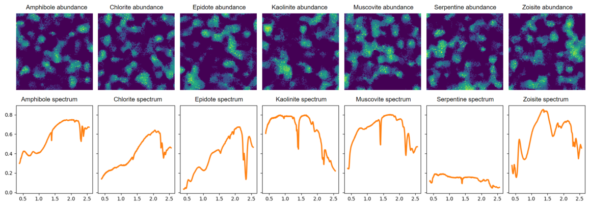
Following spectral mixing, the framework provides PCA (Principal Component Analysis)-based RGB visualization to facilitate qualitative validation of spatial structures and spectral characteristics. Figure 1 shows the overall simulated mineral abundance distribution, while Figure 2 presents the abundance distributions of individual mineral endmembers and their corresponding spectral curves in the simulated data. The final output is stored in .mat format and includes the mixed hyperspectral data cube, abundance maps, endmember instance indices, class-wise endmember sets, central endmember spectra, wavelength information, full width at half maximum (FWHM), and complete generation parameters. This comprehensive data structure enables direct application to tasks such as endmember extraction, spectral unmixing, and nonlinear mixing analysis, providing a controllable and reproducible experimental environment for algorithm evaluation and theoretical investigation.

2.1.2. Real-World Datasets

To evaluate the proposed method under realistic mineral exploration conditions, an airborne hyperspectral dataset acquired by the Shortwave Airborne Spectral Imager (SASI; ITRES, Calgary, AB, Canada) over the Liuyuan region, Gansu Province, China, was used. The SASI sensor covers the shortwave infrared region from approximately 950 to 2450 nm with 144 contiguous bands, which is suitable for detecting diagnostic absorption features of hydroxyl-bearing and carbonate minerals.

The study area is located in the Fangshankou–Liuyuan region of Guazhou County, Jiuquan City, Gansu Province, China (95°10′–95°46′E, 41°08′–41°16′N). The region is characterized by arid climatic conditions, sparse vegetation cover, and extensive rock exposure, all of which are favorable for airborne mineral mapping. Geologically, the area contains abundant metallic and non-metallic mineral occurrences and exhibits strong lithological and structural complexity, making it a representative testbed for mineral hyperspectral unmixing in natural scenes [19,20,21].

Because the study area is characterized by sparse vegetation and extensive rock exposure, the real-data experiment primarily evaluates the proposed method under exposed or weakly vegetated geological surface conditions. The effects of dense green or dry vegetation cover were not explicitly considered in the present analysis.

The airborne SASI imagery used in this study has a spatial resolution of 2.25 m. After removing spectral bands severely affected by water-vapor absorption and low signal quality, 29 effective bands were retained for analysis. These retained bands preserve the principal spectral characteristics of the target minerals while reducing noise contamination.

For real-data validation, muscovite and carbonate were selected as representative target minerals because they are widely distributed in the study area and because corresponding field and laboratory reference information is available. Field and laboratory identifications from samples DWHNG-01, DWHNG-03, DWHNG-08, DWHNG-09, LY-18-1, LY-18-2, and LY-18-3 were used as external evidence to assess the geological plausibility of the estimated endmembers and abundance maps. It should be noted that no quantitative abundance ground truth is available for the real dataset; therefore, the real-data evaluation focuses primarily on spectral consistency and geological plausibility rather than strict abundance-retrieval accuracy.

2.2. Network Architecture and Enhancements

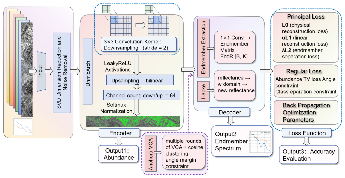
As illustrated in Figure 3, this study adopts an improved convolutional autoencoder (CAE) to construct a hyperspectral unmixing network. The overall architecture follows the encoder–decoder paradigm and is composed of three main components: an encoder, a decoder, and a loss function. Compared with conventional CAE-based unmixing models, targeted enhancements are introduced in both endmember modeling and optimization strategies to improve physical consistency, estimation stability, and the discrimination capability for spectrally similar minerals.

Nevertheless, traditional CAE-based unmixing models are often limited by insufficient physical consistency of the estimated endmembers, unstable optimization behavior, and poor discrimination of spectrally similar materials. To overcome these issues, the proposed network integrates physical models, spectral library priors, and weakly supervised constraints into the baseline CAE framework. Specifically, multi-level prior information is incorporated to guide the endmember estimation process, thereby reducing ambiguity, improving robustness, and enhancing the separability of similar mineral spectra.

Through these targeted enhancements, the proposed network is transformed from a purely data-driven architecture into a physically constrained and prior-guided hyperspectral unmixing model, while still maintaining the advantages of end-to-end training and interpretability.

The detailed network architecture configuration is summarized in

Table 1. Network architecture configuration used in the proposed hyperspectral unmixing framework.

Parameter	Description	Simulated Data	Real Data
Input dimension	Spatial–spectral size of the hyperspectral input cube	128 × 128 × 420	394 × 3287 × 29
Number of convolutional layers	Total convolution layers in encoder–decoder architecture	2 (encoder) + 1 (decoder)	2 (encoder) + 1 (decoder)
Kernel size	Convolution kernel size used in encoder and decoder	Encoder: 3 × 3	Encoder: 3 × 3
		Decoder: 1 × 1	Decoder: 1 × 1
Channel number	Number of feature channels in encoder layers	64	256
Abundance layer dimension	Dimension of the abundance output for each pixel	128 × 128 × 7	394 × 3287 × 2
Decoder form	Reconstruction module mapping abundance to reflectance	Linear 1 × 1 convolution with non-negativity constraint	Linear 1 × 1 convolution with non-negativity constraint
Setting of endmember number K	Number of endmembers used in spectral unmixing	Equal to number of simulated mineral classes	Determined from spectral library and geological prior knowledge

. The encoder consists of two convolutional layers with a stride of 1. The first layer is designed to extract local spatial–spectral features from hyperspectral images, while the second layer maps these features into pixel-wise abundance representations. To ensure the physical validity of the abundance estimates, a normalization layer based on the Softmax function is inserted between the encoder and the decoder. This layer enforces the non-negativity and sum-to-one constraints on the abundances, making the output consistent with the linear mixing model (LMM).

The decoder adopts a linear convolutional structure with non-negativity constraints, where the convolutional weights correspond to the endmember spectra. This design enables the decoder to reconstruct hyperspectral pixels through a physically interpretable linear mixing process. Within an unsupervised end-to-end training framework, the baseline CAE architecture provides a unified solution for joint endmember extraction and abundance estimation while preserving strong physical interpretability. A comprehensive summary of the network architecture and parameter configuration is provided in Table 1.

2.3. Hapke Model–Driven Endmember Modeling Constraint

The first improvement addresses the limitation of conventional CAE-based unmixing models, which perform linear reconstruction solely in the reflectance domain and neglect the nonlinear optical properties of minerals. To overcome this limitation, the Hapke radiative transfer model is embedded into the autoencoder framework, thereby introducing a physics-driven constraint for endmember modeling.

Specifically, during endmember estimation, the reflectance spectra are first transformed into the single-scattering albedo domain for modeling and then mapped back to the reflectance domain through the Hapke model. A Hapke-based reconstruction error term is explicitly incorporated into the loss function. This design integrates the nonlinear scattering characteristics of mineral surfaces into the endmember optimization process, enabling the estimated endmembers to not only numerically approximate reference spectra but also to conform to mineral optical properties in a physical sense. As a result, the realism and physical interpretability of the estimated endmember spectra are significantly enhanced.

In this study, a simplified Hapke formulation under the single-scattering approximation is adopted. Following Hapke’s reflectance theory for particulate surfaces, the nonlinear relationship between reflectance and single-scattering albedo is used to construct a Hapke-consistency constraint. The abundance-weighted single-scattering albedo is then mapped back to the reflectance domain as follows:

$$\widehat{R}=k{\displaystyle \frac{\omega }{\left(1+2m\sqrt{1-\omega }\right)\left(1+2m_0\sqrt{1-\omega }\right)+ϵ}}$$

(2)

where $\omega$ denotes the abundance-weighted single-scattering albedo, $m_0$ and $m$ are the fixed cosine terms associated with the incidence and emergence angles, respectively, $k$ is a learnable global scaling factor, and $ϵ$ is a small constant for numerical stability. In our implementation, $m_0$ = 1.0 and $m$ = 1.0 are used for both simulated and real-data experiments [18].

This fixed-geometry setting simplifies the Hapke-consistency constraint and reduces the ambiguity of jointly estimating endmembers, abundances, and reflectance reconstruction in an unsupervised framework. However, it also limits the representation of local illumination variation, surface-slope effects, viewing-geometry differences, and bidirectional reflectance variations. Therefore, the Hapke term is used as a physics-inspired consistency regularization term rather than as a full Hapke photometric inversion model.

2.4. Library-Aware Endmember Anchor–Guided Initialization and Constraint Module

To mitigate the sensitivity of end-to-end endmember learning to initialization and to prevent convergence to non-physical or unstable solutions, this study further introduces a stable initialization mechanism that integrates endmember anchor generation with library-aware constraints, providing a reasonable prior for Hapke-constrained endmember optimization. The anchor generation and spectral library matching parameters are summarized in

Table 2. Training configuration and physical modeling parameters used in the proposed network.

Parameter	Description	Simulated Data	Real Data
Training iterations	Total optimization iterations	10,000	10,000
Endmember initialization	To generate candidate anchors	Multi-run VCA (runs = 80)	FPS anchor initialization
Anchor representatives	Number of representative spectra retained per cluster	8	4
Anchor filtering threshold	Maximum spectral angle for valid anchors	10°	8°
Geometry parameter m	Hapke geometry parameter	1.0	1.0
Geometry parameter m0	Hapke illumination parameter	1.0	1.0
Hapke model type	Reflectance–albedo conversion	Simplified Hapke model	Simplified Hapke model
Learnable scaling parameter	Global scaling factor for reflectance reconstruction	Yes	Yes

.

In simulated data experiments, where the data scale is controllable and the number of endmembers is known, a multi-run Vertex Component Analysis (VCA)–based endmember anchor generation strategy is adopted. VCA is a widely used geometric endmember extraction algorithm that identifies simplex vertices in hyperspectral data under the linear mixing assumption [22]. Specifically, multiple endmember candidate sets are obtained by repeatedly applying VCA to randomly subsampled hyperspectral data. The generated candidates are first L2-normalized and then grouped into K clusters using K-means in the normalized spectral space. Within each cluster, representative spectra are selected according to their proximity to the corresponding cluster center; specifically, the candidates with the highest cosine similarity to the cluster center are retained as anchor representatives. The cluster center is further compared with the mineral spectral library using the minimum spectral angle distance (SAD). Each cluster is assigned to the mineral class with the smallest SAD, while clusters whose minimum SAD exceeds the predefined threshold are discarded. Through this process, representative and physically meaningful endmember anchor sets are constructed for each mineral class. This strategy effectively alleviates the sensitivity of single-run VCA to noise and initialization and prevents unconstrained drift of endmember candidates in high-dimensional spectral space.

For real hyperspectral data experiments, considering the large data volume and high spectral dimensionality, VCA faces practical limitations in terms of computational complexity and scalability. Therefore, a Farthest Point Sampling (Farthest Point Sampling, FPS)–based endmember anchor generation method is employed. FPS iteratively selects samples that are maximally distant in spectral space, ensuring diversity and coverage of endmember candidates with relatively low computational cost. Subsequently, the FPS-generated candidates are assigned to mineral classes according to the minimum SAD between each candidate and the corresponding spectral library entries. A fixed number of representative anchors is retained for each mineral class, thereby achieving a balance between spectral diversity and library consistency of the selected anchors.

It should be emphasized that, regardless of whether VCA or FPS is employed, the generated endmember anchors are not directly used as the final endmember results. Instead, they are introduced into subsequent network training as library-aware soft prior constraints. During endmember optimization, spectral consistency constraints between the network-estimated endmembers and their corresponding anchor sets are enforced to guide the search direction and effectively restrict the endmember search space. Without altering the core network architecture, this mechanism significantly improves the convergence stability, physical consistency, and robustness of endmember estimation.

2.5. Loss Function

To jointly optimize endmember spectra and abundance distributions while incorporating physical constraints and prior information, a composite loss function is constructed. The overall objective function is defined as

$$L=L_{\mathrm{rec}}+{\lambda }_{\mathrm{hapke}}{L}_{\mathrm{hapke}}+{\lambda }_{\mathrm{anc}}{L}_{\mathrm{anchur}}+{\lambda }_{\mathrm{reg}}{L}_{\mathrm{reg}}$$

(3)

where L_rec denotes the reconstruction loss, L_hapke represents the Hapke model consistency loss, L_anchor enforces spectral consistency with anchor endmembers, L_reg is the abundance regularization term.

The reconstruction loss measures the discrepancy between the observed hyperspectral reflectance X and the reconstructed spectra $\widehat{X}$ produced by the decoder:

$$L_{rec}=\left|\right|X-\widehat{X}|{|}_2^2$$

(4)

In this study, the squared Euclidean distance is adopted to ensure stable gradient propagation during optimization.

The Hapke consistency loss introduces a physics-based constraint by enforcing consistency between the reconstructed reflectance and the reflectance generated through the Hapke radiative transfer model. This mechanism allows the estimated endmembers to conform to the nonlinear scattering characteristics of particulate mineral surfaces.

To incorporate physical scattering characteristics, the reconstructed reflectance is constrained to be consistent with the reflectance generated through the Hapke radiative transfer model. The Hapke-consistency loss is defined as

$$L_{hapke}=\left|\right|R_{obs}-R_{hapke}(\omega )|{|}_2^2$$

(5)

where R_obs denotes the observed reflectance and R_hapke(ω) represents the reflectance reconstructed from the estimated single-scattering albedo ω using the simplified Hapke model.

This constraint enforces physical plausibility of the estimated endmember spectra under nonlinear mineral scattering conditions.

To integrate spectral prior knowledge, anchor spectra derived from the spectral library are incorporated as weak supervision. The anchor matching loss is formulated as

$$L_{anchor}={\displaystyle {\displaystyle \sum }_{k=1}^K}SAD\left(e_k,a_k\right)$$

(6)

where e_k denotes the k-th estimated endmember spectrum, a_k represents the corresponding anchor spectrum, and SAD is the spectral angle distance defined as

$$SAD\left(e,a\right)=\arccos \left({\displaystyle \frac{e^{T}a}{\parallel e\parallel \parallel a\parallel }}\right)$$

(7)

This term guides the optimization toward spectrally meaningful and physically interpretable endmembers.

Finally, a spatial regularization term is introduced to promote smoothness in the abundance maps:

$$L_{reg}=TV\left(A\right)$$

(8)

where TV denotes the total variation operator applied to the abundance maps A. This regularization suppresses noise-induced fluctuations and improves spatial consistency.

The weighting parameters for different loss components are summarized in

Table 3. Loss weighting parameters used in the proposed method.

Loss Component	Symbol	Simulated Data	Real Data
Reconstruction loss	Lrec	1.0	1.0
Hapke Consistency loss	Lhapke	0.5	0.5
Anchor Consistency loss	Lanchor	0.2	0.2
Abundance regularization	Lreg	1 × 10−3	1 × 10−3

.

3. Results

To validate the effectiveness of the proposed hyperspectral mineral mixed-pixel unmixing method based on the convolutional autoencoder and its improved variants, experiments were conducted on both simulated datasets and real hyperspectral datasets. By jointly analyzing endmember estimation accuracy, abundance inversion results, and their physical consistency, the performance and stability of the proposed model were systematically evaluated.

3.1. Experimental Results and Analysis on Simulated Data

3.1.1. Comparative Analysis of Endmember Estimation Results

Simulated data experiments were conducted to quantitatively and qualitatively evaluate the endmember extraction performance of different unmixing methods under conditions where the true endmembers and abundance maps are known.

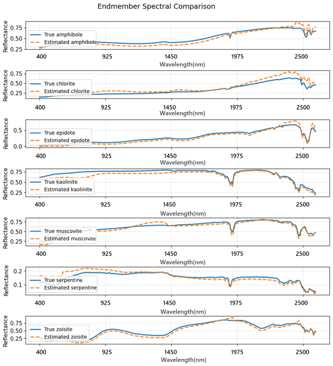
Figure 4 shows the endmember spectra estimated by the proposed method, together with the corresponding ground-truth spectra. Overall, the estimated spectra exhibit high consistency with the reference across the entire spectral range, especially at major absorption features. Both the positions and shapes of these features are well preserved, indicating high spectral fidelity.

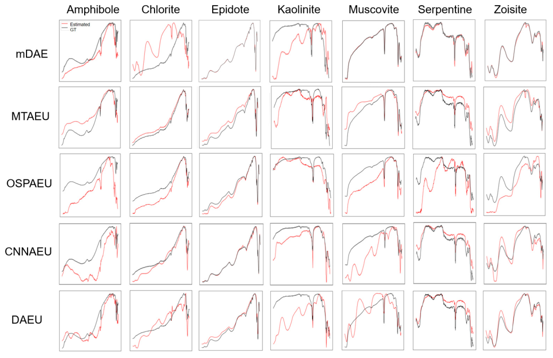
Figure 5 shows the spectral extraction results of various other unmixing methods [23,24,25,26]. As shown in the figure, compared with the competing methods, the proposed approach generally yields spectra that are closer to the references and abundance maps with fewer noisy artifacts. The improvement is particularly noticeable for minerals with similar spectral characteristics, such as chlorite and muscovite.

3.1.2. Analysis of Abundance Inversion Accuracy and Spatial Consistency

Simulated data experiments were conducted to evaluate the abundance estimation performance of different unmixing methods under controlled conditions where the ground-truth abundance maps are known.

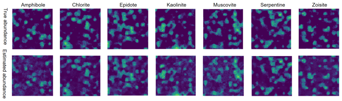
Figure 6 illustrates the abundance maps generated by the proposed method, along with the corresponding ground-truth distributions. As can be observed, the proposed approach produces abundance maps with clear spatial structures and strong regional consistency. In highly mixed regions and endmember transition zones, the abundance variations remain smooth and closely follow the predefined ground-truth patterns, indicating reasonably stable spatial modeling capability.

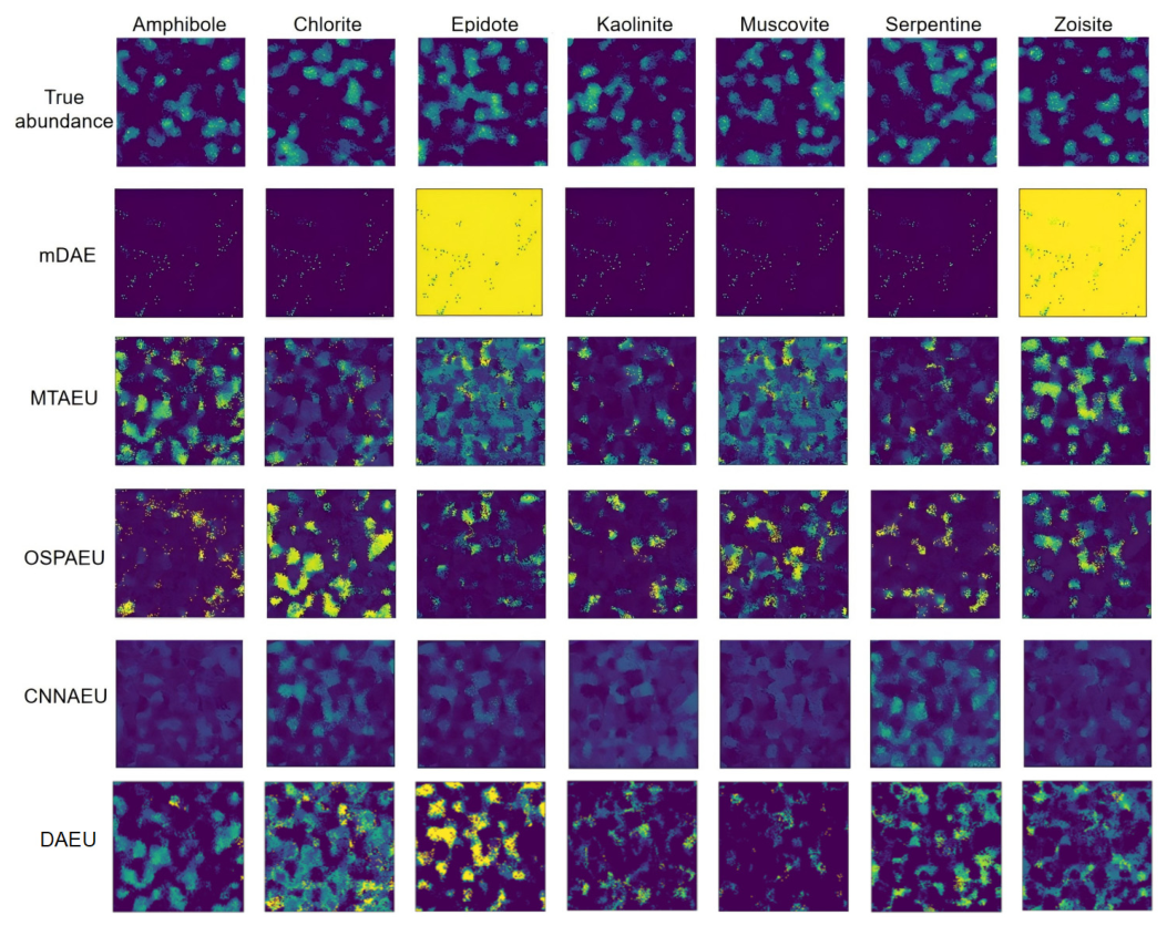
Figure 7 further presents a visual comparison of abundance extraction results between our method and other approaches. The competing methods preserve the overall spatial pattern to varying degrees, but their abundance maps tend to contain more fragmented structures or spurious fluctuations in highly mixed regions.

The detailed per-mineral Endmember SAD and Abundance RMSE of the proposed method on synthetic data are reported in

Table 4. Comparison of Endmember SAD and Abundance RMSE for different methods.

Methods	Endmember SAD	Abundance RMSE
mDAE	6.3228 ± 4.5591	0.3256 ± 0.1057
MTAEU	5.9184 ± 2.5154	0.1959 ± 0.0947
OSPAEU	7.2461 ± 0.0894	0.2364 ± 0.1025
CNNAEU	4.5381 ± 0.8223	0.1945 ± 0.0278
DAEU	5.8669 ± 2.2206	0.2030 ± 0.0803
Ours	3.7714 ± 1.3011	0.0585 ± 0.0252

Data are presented as mean ± standard deviation (SD).

.

Table 5. Per-Mineral Endmember SAD and Abundance RMSE of the proposed method on simulated data.

Endmember-Wise Metrics	Endmember SAD	Abundance RMSE
Amphibole	2.5706	0.0576
Chlorite	5.1555	0.0420
Epidote	4.3869	0.0676
Kaolinite	2.8607	0.1052
Muscovite	3.6917	0.0686
Serpentine	5.7290	0.0384
Zoisite	2.0851	0.0301
Overall Average	3.7714	0.0585

below presents the quantitative analysis results of our proposed method, including SAD (Spectral Angle Distance) and RMSE (Root Mean Square Error) metrics. Quantitative evaluations further confirm the superiority of the proposed method. Specifically, it achieves the lowest abundance root mean square error (RMSE) among all compared methods, demonstrating higher accuracy and stronger stability in abundance inversion.

3.1.3. Ablation Study and Model Robustness Analysis

To further investigate the contribution of key modules to model performance, an ablation study and robustness analysis were conducted on the simulated data. By progressively removing or disabling different enhanced modules from the base network, multiple control models were constructed, and their endmember estimation and abundance inversion performances were systematically compared.

The ablation experimental results are shown in

Table 6. Ablation Study on SAD.

Mineral Type/ Remove Module	Hapke	Anchor	Hapke and Anchor	Ours
Amphibole	7.1670	3.2424	8.2626	2.5706
Chlorite	6.2859	5.6171	6.8956	5.1555
Epidote	11.5257	5.3473	8.1164	4.3869
Kaolinite	5.3283	7.9018	8.0359	2.8607
Muscovite	4.6663	4.8595	5.0122	3.6917
Serpentine	13.5913	9.2710	15.0064	5.7290
Zoisite	6.2742	3.6059	5.4546	2.0851
Overall Average	7.8341	5.6921	8.1120	3.7828

and

Table 7. Ablation Study on RMSE.

Mineral Type/ Remove Module	Hapke	Anchor	Hapke and Anchor	Ours
Amphibole	0.1361	0.1361	0.1378	0.0576
Chlorite	0.1546	0.1888	0.1996	0.0420
Epidote	0.0981	0.1494	0.2256	0.0676
Kaolinite	0.1259	0.1660	0.2020	0.1052
Muscovite	0.1432	0.1631	0.1598	0.0686
Serpentine	0.1680	0.1737	0.2122	0.0384
Zoisite	0.1035	0.1078	0.1066	0.0301
Overall Average	0.1328	0.1550	0.1777	0.0585

. When the Hapke physical model constraint is removed, the estimated endmember spectra exhibit noticeable deviations in certain spectral bands, particularly in absorption regions associated with nonlinear scattering effects, leading to a significant reduction in the physical plausibility of the endmember estimates. This highlights the importance of incorporating physical model constraints to improve the realism and interpretability of endmember spectra. On the other hand, when the library-aware endmember anchor guidance module is removed, the endmember estimation results show greater variability across experimental runs, and the abundance inversion errors increase, suggesting that the anchor priors play a critical role in stabilizing the end-to-end endmember learning process and preventing physically implausible solutions.

3.2. Application on Real Data

To evaluate the performance of the proposed network on real-world hyperspectral data, experiments were conducted using the SASI datasets. The evaluation focused on the network’s ability to accurately extract endmembers corresponding to known mineral classes under realistic imaging conditions, where sensor noise, illumination variations, and mixed pixels are present. The natural mixing of minerals in real scenes increases the difficulty of discrimination. In addition, uncontrollable noise and spatial heterogeneity further complicate the extraction process, resulting in slightly lower performance compared with simulated datasets.

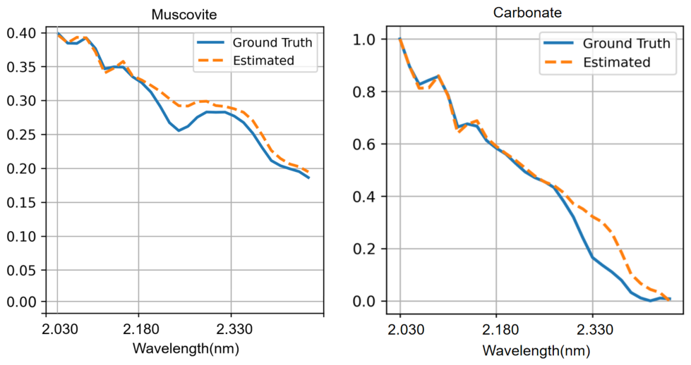
Figure 8 shows the estimated spectra of two typical minerals in comparison with reference spectra from the ground truth library. In this study, the ground truth spectral library refers to mineral spectra collected from field measurements and used as reference spectra for evaluation. The proposed network effectively captures the main absorption features of each mineral, and the overall spectral shapes closely match the references. Minor discrepancies are observed in high-frequency variations or subtle absorption features, which may be attributed to noise, spatial heterogeneity, or spectral similarity caused by mineral mixing. Nonetheless, the results indicate that the network can generate physically plausible endmembers in real data scenarios.

Quantitative evaluation was performed using the spectral angle distance (SAD) between the estimated endmembers and the reference spectra. The results are shown in

Table 8. Endmember-wise metrics on the real data.

Endmember-Wise Metrics	Baseline SAD	Ours SAD
Muscovite	6.9596	3.6717
Carbonate	17.1543	3.1970
Overall Average	12.0570	3.4344

. The proposed method achieves low SAD values on average, indicating higher spectral consistency and improved physical interpretability. Additionally, the variance of SAD across multiple runs is reduced, demonstrating the robustness of the model against initialization sensitivity and local minima issues that commonly affect unsupervised endmember extraction.

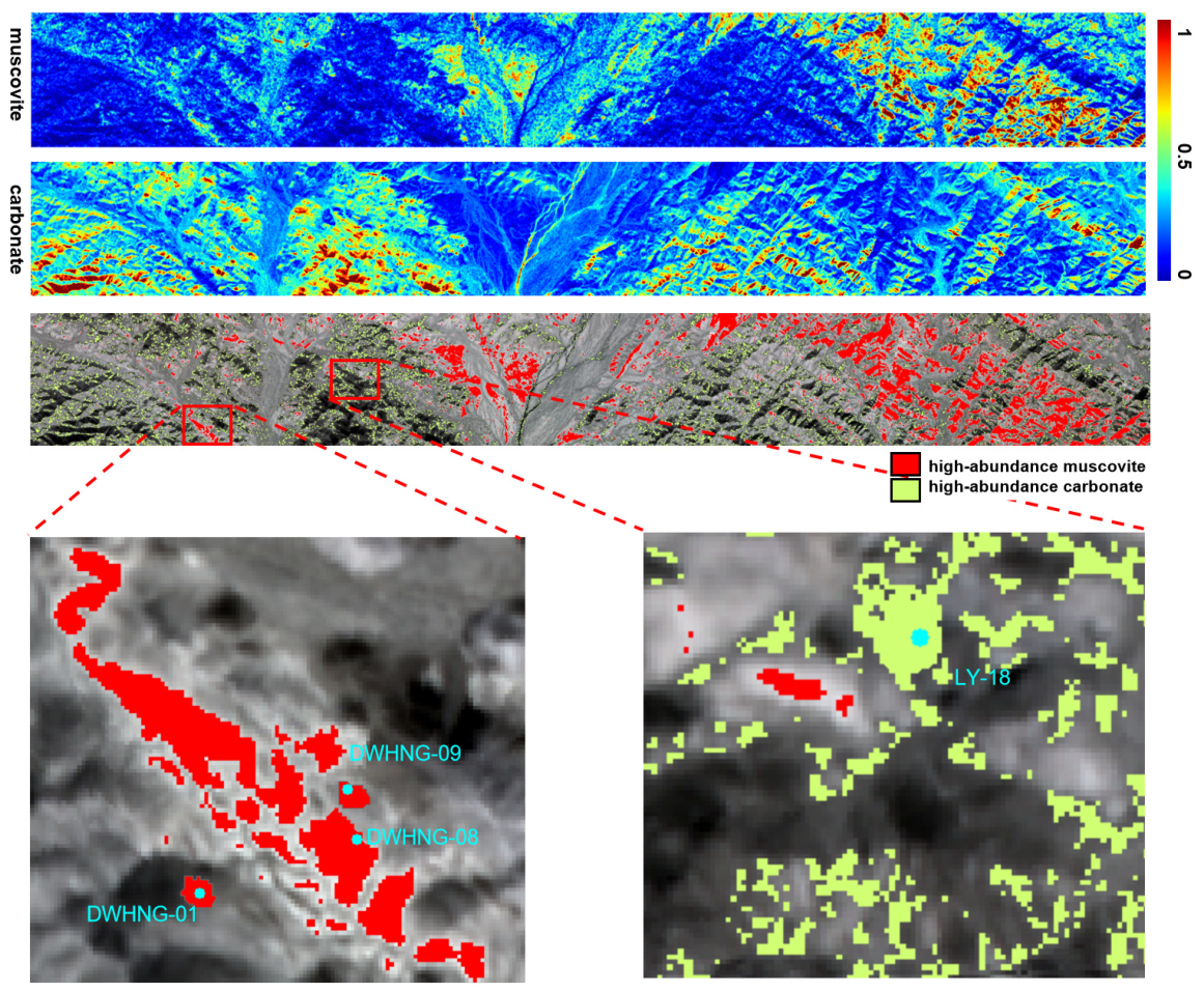
Figure 9 shows the predicted abundance map of muscovite and carbonate minerals in the study area. In this experiment, the proposed method was applied to real airborne hyperspectral imagery, and two representative minerals—muscovite and carbonate—that are widely distributed across the study area were selected for validation. The results were validated using field and laboratory rock identification data from the Hebei Geological Survey Institute (samples DWHNG-01, DWHNG-03, DWHNG-08, and DWHNG-09) and the National Building Materials Geological Engineering Institute (samples LY-18-1, LY-18-2, and LY-18-3). As shown in

Table 9. The main mineral types of samples DWHNG-01, DWHNG-03, DWHNG-08, and DWHNG-09.

Sampling Point	DWHNG-01	DWHNG-08	DWHNG-09
Main minerals	Muscovite, calcite, chlorite, kaolinite, etc.	Muscovite, calcite, pyrophyllite, etc.	Muscovite, dolomite, etc.

and

Table 10. The main mineral types and images of samples LY-18-1, LY-18-2 and LY-18-3.

Sampling Point	LY-18-1	LY-18-2	LY-18-3
Figure
Main minerals	Calcite, serpentine, and a small amount of other carbonates	Calcite, serpentine, and a small amount of other carbonates	Calcite, dolomite, and a small amount of other carbonates

. The network successfully captures the main muscovite-rich and carbonate-rich alteration zones, with the highest predicted abundances concentrated in areas where these minerals are dominant, showing strong consistency with field observations.

In regions characterized by natural mineral mixing, muscovite and carbonate exhibit clear dominance patterns, indicating that the network can effectively handle mixed pixels. The abundance map shows spatially coherent patterns with gradual changes between mineral zones, while preserving the main geological structures. Local variations reflect true transitions rather than artifacts introduced by the unmixing process.

These results suggest that the proposed network can jointly recover muscovite- and carbonate-related endmember signatures and generate abundance patterns that are more compatible with field observations and known geological structures.

It should be noted that the carbonate endmember extracted from the real SASI data is used to represent carbonate-related mineral responses in the study area, rather than to further discriminate specific carbonate species. Carbonate minerals generally exhibit similar absorption characteristics in the SWIR region, particularly beyond 2000 nm. Considering the limited number of effective SASI bands retained after preprocessing, spectral mixing effects, and the absence of pixel-level quantitative mineral abundance ground truth, reliable species-level discrimination among carbonate minerals is beyond the scope of the current experiment. Therefore, the predicted carbonate abundance map is interpreted by comparing its high-value regions with the carbonate-bearing sampling points listed in Table 9 and Table 10. The general spatial consistency between these sampling records and the predicted carbonate abundance distribution supports the geological plausibility of the extracted carbonate component.

Overall, the model shows promising transferability from simulated to real airborne datasets, while the real-data results should still be interpreted primarily in terms of spectral consistency and geological plausibility rather than strict abundance accuracy.

4. Discussion and Conclusions

This study proposed a physically constrained and library-guided convolutional autoencoder framework for mineral hyperspectral unmixing. The method preserves the interpretability of a linear abundance–endmember reconstruction backbone while incorporating a Hapke-consistency regularization term and a library-aware anchor module to improve endmember optimization.

Experiments on simulated datasets showed that the proposed framework achieved improved endmember spectral fidelity and lower abundance estimation error than several representative autoencoder-based baselines. The performance gain was more evident under nonlinear mixing conditions, suggesting that the introduced physical constraint is particularly beneficial when intimate mineral mixing weakens the validity of linear assumptions. Ablation analysis further indicated that the Hapke-consistency term mainly contributes to physical plausibility, whereas the anchor module mainly improves optimization stability and spectral consistency.

Experiments on real airborne SASI data from the Liuyuan area showed that the proposed method generated endmember spectra that were more consistent with field and laboratory mineral references and produced abundance maps with improved spatial coherence. Because pixel-level quantitative abundance ground truth is unavailable for the real SASI dataset, the field and laboratory sampling records were used only as independent reference information for geological plausibility assessment. Therefore, the real-data results are interpreted mainly from the perspectives of continuous abundance patterns, endmember spectral consistency, and geological plausibility, rather than strict quantitative abundance accuracy.

Vegetation cover remains a major challenge for large-scale mineralogical remote sensing. Both green and dry vegetation can obscure exposed mineral surfaces and introduce wavelength-dependent nonlinear mixing effects associated with canopy structure, moisture content, shadowing, and background soil–rock interactions. In the present study, vegetation was not explicitly modeled as an endmember, nor was a canopy radiative transfer component incorporated. Accordingly, the real-data validation should be interpreted as most applicable to arid and sparsely vegetated geological environments. Future work should incorporate vegetation endmembers, masking strategies, or coupled canopy–mineral radiative transfer constraints to extend the applicability of the proposed framework to more densely vegetated regions.

Overall, the proposed framework demonstrates that integrating physically motivated constraints and spectral-library priors into deep autoencoder-based unmixing can improve the robustness and interpretability of mineral hyperspectral unmixing. Future work should further investigate more complete radiative transfer constraints, adaptive anchor-selection strategies, and more extensive real-world validation in geologically complex mineral systems.

References

1. Li, Z.; Ma, Z.; van der Kuijp, T.J.; Yuan, Z.; Huang, L. A review of soil heavy metal pollution from mines in China: Pollution and health risk assessment. Sci. Total Environ. 2014, 468–469, 843–853. [Google Scholar] [CrossRef]
2. European Commission. 100 Radical Innovation Breakthroughs for the Future; Publications Office of the European Union: Brussels, Belgium, 2019; p. 66. [CrossRef]
3. National Academies of Sciences Engineering and Medicine. Thriving on Our Changing Planet: A Decadal Strategy for Earth Observation from Space; The National Academies Press: Washington, DC, USA, 2018; p. 549. [Google Scholar] [CrossRef]
4. Nie, M.; Liu, Z.; He, X.; Qiu, Q.; Zhang, Y.; Chang, J. End-member extraction based on segmented vertex component analysis in hyperspectral images. Appl. Opt. 2017, 56, 2476–2482. [Google Scholar] [CrossRef]
5. Sahoo, M.M.; Kalimuthu, R.; PV, A.; Porwal, A.; Mathew, S.K. Modelling Spectral Unmixing of Geological Mixtures: An Experimental Study Using Rock Samples. Remote Sens. 2023, 15, 3300. [Google Scholar] [CrossRef]
6. Zhang, M.; Yang, M.; Xie, H.; Yue, P.; Zhang, W.; Jiao, Q.; Xu, L.; Tan, X. A Global Spatial-Spectral Feature Fused Autoencoder for Nonlinear Hyperspectral Unmixing. Remote Sens. 2024, 16, 3149. [Google Scholar] [CrossRef]
7. Keshava, N.; Mustard, J.F. Spectral unmixing. IEEE Signal Process. Mag. 2002, 19, 44–57. [Google Scholar] [CrossRef]
8. Sun, L.; Wu, F.; Zhan, T.; Liu, W.; Wang, J.; Jeon, B. Weighted Nonlocal Low-Rank Tensor Decomposition Method for Sparse Unmixing of Hyperspectral Images. IEEE J. Sel. Top. Appl. Earth Obs. Remote Sens. 2020, 13, 1174–1188. [Google Scholar] [CrossRef]
9. Su, Y.; Xu, R.; Gao, L.; Han, Z.; Sun, X. Development of deep learning-based hyperspectral remote sensing image unmixing. Natl. Remote Sens. Bull. 2024, 28, 1–19. [Google Scholar] [CrossRef]
10. Qin, K.; Hao, Y.; Zhao, Y.; Cui, X.; Yang, Y.; Zhu, L.; Tian, Q. A survey on hyperspectral remote sensing unmixing techniques based on autoencoders. Infrared Laser Eng. 2025, 54, 30–47. [Google Scholar] [CrossRef]
11. Georgiev, D.; Fernández-Galiana, Á.; Vilms Pedersen, S.; Papadopoulos, G.; Xie, R.; Stevens, M.M.; Barahona, M. Hyperspectral unmixing for Raman spectroscopy via physics-constrained autoencoders. Proc. Natl. Acad. Sci. USA 2024, 121, e2407439121. [Google Scholar] [CrossRef]
12. Kannan, R.; Ievlev, A.V.; Laanait, N.; Ziatdinov, M.A.; Vasudevan, R.K.; Jesse, S.; Kalinin, S.V. Deep data analysis via physically constrained linear unmixing: Universal framework, domain examples, and a community-wide platform. Adv. Struct. Chem. Imaging 2018, 4, 6. [Google Scholar] [CrossRef] [PubMed]
13. Liu, X.; Duan, C.; Cai, W.; Shao, X. Unmixing Autoencoder for Image Reconstruction from Hyperspectral Data. Anal. Chem. 2024, 96, 20354–20361. [Google Scholar] [CrossRef] [PubMed]
14. Kaufman, L.; Rousseeuw, P.J. Finding Groups in Data, 1st ed.; Wiley: New York, NY, USA, 1990; pp. 68–125. [Google Scholar] [CrossRef]
15. Dobigeon, N.; Tourneret, J.Y.; Richard, C.; Bermudez, J.C.M.; McLaughlin, S.; Hero, A.O. Nonlinear Unmixing of Hyperspectral Images: Models and Algorithms. IEEE Signal Process. Mag. 2014, 31, 82–94. [Google Scholar] [CrossRef]
16. Ferguson, T.S. A Bayesian Analysis of Some Nonparametric Problems. Ann. Stat. 1973, 1, 209–230. [Google Scholar] [CrossRef]
17. Howari, F.M.; Acbas, G.; Nazzal, Y.; AlAydaroos, F. Hapke-based computational method to enable unmixing of hyperspectral data of common salts. Chem. Cent. J. 2018, 12, 90. [Google Scholar] [CrossRef]
18. Hapke, B. Bidirectional reflectance spectroscopy: 4. The extinction coefficient and the opposition effect. Icarus 1986, 67, 264–280. [Google Scholar] [CrossRef]
19. Liu, D.; Tian, F.; Qiu, J.; Ye, F.; Yan, B.; Sun, Y.; Wang, Z. Application of Hyperspectral Remote Sensing in Solid Ore Exploration in the Liuyuan-Fangshankou Area. Acta Geol. Sin. 2017, 91, 2781–2795. [Google Scholar] [CrossRef]
20. Liu, D.; Ye, F.; Zhao, Y.; Tian, F.; Qiu, J. Airborne Hyperspectral Remote Sensing for Gold Prospecting Around Liuyuan-Fangshankou Area, Gansu Province, China. Geo-Inf. Sci. 2015, 17, 1545–1553. [Google Scholar] [CrossRef]
21. Liu, D.; Zhao, Y.; Ye, F.; Tian, F.; Qiu, J. Study on the metallogenic background of the Liuyuan–Fangshankou area by using airborne hyperspectral remote sensing. Remote Sens. 2017, 21, 136–148. [Google Scholar] [CrossRef]
22. Nascimento, J.M.P.; Dias, J.M.B. Vertex component analysis: A fast algorithm to unmix hyperspectral data. IEEE Trans. Geosci. Remote Sens. 2005, 43, 898–910. [Google Scholar] [CrossRef]
23. Dou, Z.; Gao, K.; Zhang, X.; Wang, H.; Wang, J. Hyperspectral Unmixing Using Orthogonal Sparse Prior-Based Autoencoder with Hyper-Laplacian Loss and Data-Driven Outlier Detection. IEEE Trans. Geosci. Remote Sens. 2020, 58, 6550–6564. [Google Scholar] [CrossRef]
24. Guo, R.; Wang, W.; Qi, H. Hyperspectral image unmixing using autoencoder cascade. In Proceedings of the 2015 7th Workshop on Hyperspectral Image and Signal Processing: Evolution in Remote Sensing, Tokyo, Japan, 2–5 June 2015. [Google Scholar] [CrossRef]
25. Palsson, B.; Sveinsson, J.R.; Ulfarsson, M.O. Spectral-Spatial Hyperspectral Unmixing Using Multitask Learning. IEEE Access 2019, 7, 148861–148872. [Google Scholar] [CrossRef]
26. Palsson, B.; Ulfarsson, M.O.; Sveinsson, J.R. Convolutional Autoencoder for Spectral–Spatial Hyperspectral Unmixing. IEEE Trans. Geosci. Remote Sens. 2021, 59, 535–549. [Google Scholar] [CrossRef]
Figure 1. Simulated mineral abundance distribution.
Remotesensing 18 01723 g001
Figure 2. Distribution of mineral endmember abundance and spectral curve of simulated data.
Remotesensing 18 01723 g002
Figure 3. Network architecture diagram. SVD: Singular Value Decomposition, used for dimensionality reduction and feature extraction.
Remotesensing 18 01723 g003
Figure 4. Comparison between estimated and reference endmember spectra.
Remotesensing 18 01723 g004
Figure 5. Comparison between the estimated endmember spectrum and the real endmember spectrum by the existing methods.
Remotesensing 18 01723 g005
Figure 6. Comparison between estimated and reference endmember abundance.
Remotesensing 18 01723 g006
Figure 7. Comparison between the estimated endmember abundance and the real endmember abundance by the existing methods.
Remotesensing 18 01723 g007
Figure 8. Comparison between estimated and reference endmember.
Remotesensing 18 01723 g008
Figure 9. Continuous estimated abundance maps and local geological plausibility assessment of muscovite and carbonate in the SASI study area. The upper two panels show the continuous estimated abundance proportions of muscovite and carbonate generated by the proposed model and normalized to 0–1. The middle panel overlays high-abundance muscovite and carbonate regions on the grayscale SASI background for spatial reference. The lower panels show enlarged local views around representative sampling points.
Remotesensing 18 01723 g009