Multi-Decadal Evolution Pattern and Trends of the Central Coastline of Jiangsu Province: Implications for Future Coastal Management

Highlights

What are the main findings?

• The spatiotemporal changes followed a distinct pattern with the Sheyang estuary as the boundary, characterized by “more erosion in the north and more accretion in the south.”
• The coastline evolution processes were classified into seven distinct patterns, each with clear differences in spatial distribution and state transitions.

What are the implications of the main findings?

• The study indicates that ongoing sediment reduction, rising sea levels, and the increased frequency of extreme marine storms have heightened the risk of coastal erosion. This implies a growing threat to coastal communities, infrastructure, and ecosystems in the area.
• Findings provide actionable insights for sustainable management and protection of muddy coasts globally.

Abstract

As an important geographical component at the boundary between land and ocean, the coastline serves as a key indicator reflecting coastal erosion and ecosystem variations. The central Jiangsu coast is a typical muddy coast, and against the backdrop of global climate change and large-scale coastal development, its coastal evolution is complex. In this study, we analyzed the patterns and trends in the evolution of Jiangsu’s coastline using remote sensing imagery from 1984 to 2024. The result indicated that the coastline length in central Jiangsu exhibits a trend of ‘initial continuous decrease followed by recovery growth.’ The coastline peaked at approximately 586.5 km in 1988 and then shortened to a minimum of about 365.2 km in 2015, after which it began to recover. Throughout the study period, the spatiotemporal changes in the coastline displayed a pattern with the Sheyang Estuary as the boundary, characterized by ‘more erosion in the north and more accretion in the south.’ The most severely eroded section was near the Fansheng Estuary, retreating by about 1412.18 m, whereas the most significant sedimentation occurred north of Fangtang Estuary, advancing by about 11,129.78 m toward the sea, with appositional uncertainty (RMSE) of ±15.6 m based on independent validation. The coastline evolution process was classified into seven patterns, with clear differences in spatial distribution and state transitions among them. With the sediment reduction, rising sea levels, and increased frequency of extreme marine storms has heightened the risk of coastal erosion. Therefore, measures such as comprehensive protection, restoration, and management of muddy coasts, scientific promotion of sedimentation, and appropriate reclamation design should be implemented.

1. Introduction

Coastal zones are important interfaces between the ocean and land, because they offer abundant, biologically diverse, and productive ecosystems, providing important ecological services for fish, birds, and other organisms [1,2]. Therefore, it is one of the most densely populated regions in the world and features the most energetic and frequent human activities. According to statistics, approximately 65% of the global population living in cities with populations exceeding 5 million is located in coastal, low-lying areas at altitudes of less than 10 m [3,4,5]. However, over the past few decades, due to severe threats from global climate change, sea level rise, storms, floods, and human activities (such as population growth, rapid urbanization, and development pressure, etc.), the coastal zone system has undergone significant changes, including coastal erosion damage, loss of biological habitats, reduction in biodiversity, and decline in productivity [6,7,8]. Moreover, the growing population and intensifying climate change have exacerbated these threats [9]. However, the characteristics of the coastline depend on the interactions among waves, tides, rivers, storms, dynamic structures, and physical processes, and these play an important role in indicating sea-level rise, coastal erosion, wetland ecological resources, and nearshore environmental conditions [10,11]. Therefore, monitoring the dynamic changes and evolutionary patterns of coastal morphology is of great significance for coastal zone conservation and environmental management, helping to further assess the stability or vulnerability of coastal areas and to better guide the sustainable management of coastal regions.

The key to monitoring and responding to coastal migration and reclamation activities lies in obtaining reliable, timely data and methods [12]. Compared with traditional techniques, remote sensing monitoring technology combined with geographic information systems (GIS) is widely used for coastline extraction, monitoring, and long-term land use classification [13,14,15] because of its macro, rapid, real-time, and dynamic characteristics, as well as advantages like wide coverage, high efficiency, and low cost. Therefore, these new technological tools provide strong support for studying spatiotemporal changes in coastlines and offer unprecedented free data sources. Currently, many researchers are combining methods such as remote sensing and GIS to capture and extract coastline information. For example, synthetic aperture radar (SAR) images are used to extract coastlines via segmentation methods [16,17,18] because SAR imagery is insensitive to weather conditions such as clouds or fog and is effective for target detection. However, the effectiveness of SAR data for coastline extraction may be affected by flat surfaces such as mudflats or fine sandy beaches, as their low backscatter is similar to that of surface water [16,19]. Secondly, optical imagery, owing to its high land reflectance and low water reflectance, can clearly distinguish land from water. Coastlines can be extracted by calculating the Normalized Difference Vegetation Index (NDVI) [20], the Normalized Difference Water Index (NDWI) [21,22,23], and the Modified Normalized Difference Water Index (MNDWI) [24], using image classification tools, and machine learning models [25]. However, it may be affected by clouds, cloud shadows, buildings, and mountains, as well as reflections from the seabed and nearby land [26,27]. Thirdly, using UAV-mounted LiDAR, which provides high spatiotemporal resolution, enables rapid monitoring of coastlines [28,29]. However, this method is sensitive to environmental conditions such as strong winds, rainfall, and thick fog, which may affect flight safety and data quality. The costs of equipment purchase, maintenance, and data processing are relatively high, and the professional technical requirements for operators are also high. The coverage of a single flight is limited. For large-scale coastline monitoring, multiple flights and complex data splicing are required.

The central coast of Jiangsu Province is one of the most typical muddy coasts in China, characterized by vast muddy tidal flats with a slope of only about 3‰ and widths of several kilometers, and it is rich in resources from these tidal flats. The central coast of Jiangsu faces multiple pressures, primarily due to reduced riverine sediment input. Since 1128, when the Yellow River changed its course to flow into the sea through northern Jiangsu, it brought a large amount of sediment, causing the coast of Jiangsu to advance rapidly towards the sea at an average rate of 0.2–0.3 km/yr [30]. However, since 1855, the dominant coastal processes have changed significantly due to the Yellow River’s northward migration into the Bohai Sea and a decrease in riverine sediment supply, resulting in coastal erosion and retreat. Moreover, human activities, including direct coastal activities and reclamation, as well as sea-level rise, changes in wind and wave conditions, and intensification of extreme events, have also been important factors influencing coastal changes, leading to a series of adverse consequences such as loss of land and biological habitats, coastal erosion, and damage to infrastructure and buildings [31,32]. Numerous studies have been conducted along the Jiangsu coast, focusing on coastal sediment dynamics, coastal evolution, and coastal environmental change [32,33,34]. Recently, studies based on remote sensing to monitor the changes in the coastline of Jiangsu and its surrounding areas have been carried out, but most of them are merely based on coastline extraction methods [35,36,37], coastal land use, and coastal stability [34,38,39]. Although many studies have examined coastline change using remote sensing, most focus on specific sections or regions of the coastline. However, relatively few studies address the long-term evolution of coastal patterns and trends, and there is a lack of systematic, comprehensive analyses from multiple perspectives. Therefore, the muddy coast in central Jiangsu Province was selected as the study area. Using Landsat and Sentinel images from 1986 to 2024, along with ENVI and ArcGIS software, the study investigated dynamic changes in the coastline driven by various factors, patterns of evolution, and future trends. The aims of this study are to: (1) analyze the long-term rate and intensity of coastline changes in central Jiangsu Province over the past 38 years; (2) identify the evolution patterns and influencing factors; and (3) assess potential coastline risks and develop targeted management strategies. This study contributes by integrating multi-decadal shoreline analysis, evolution-pattern clustering, and data-driven prediction within a highly dynamic muddy-coast system. The study particularly emphasizes the coupling between natural sedimentary processes and anthropogenic coastal reshaping, providing new insights into the evolution of engineered muddy coasts.

2. Materials and Methods

2.1. Study Area

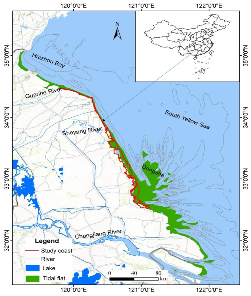
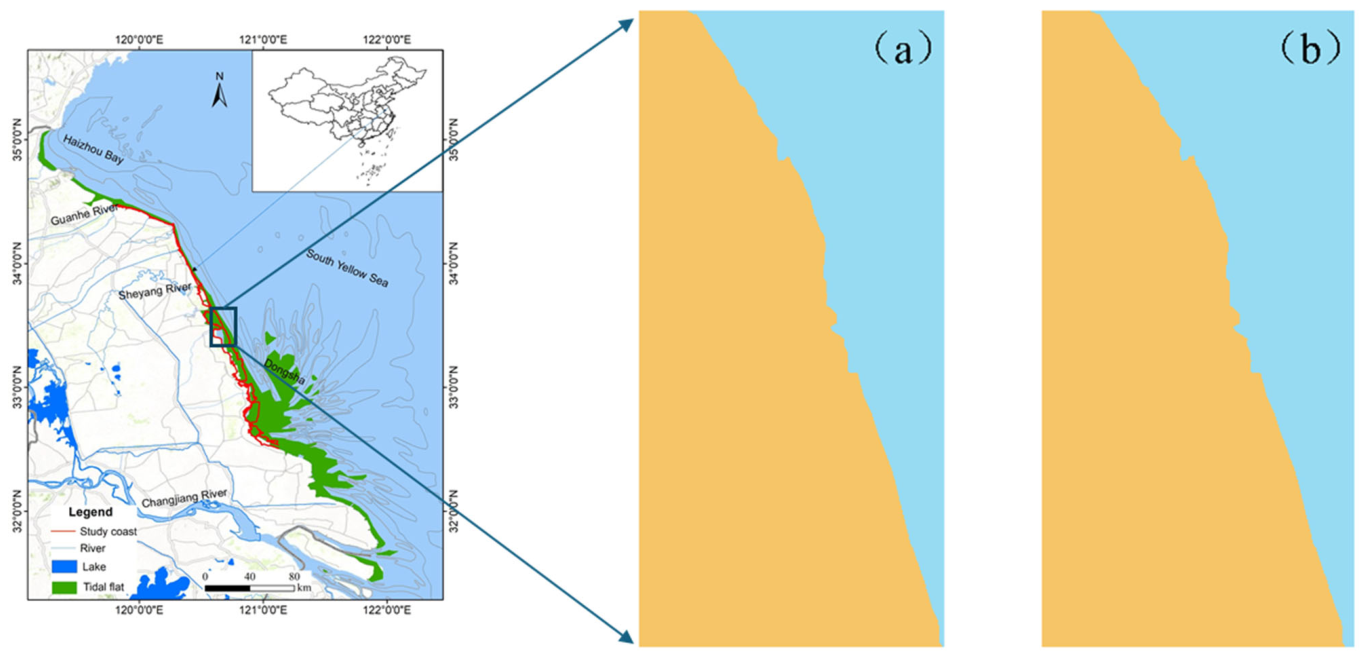
The central coast of Jiangsu Province is located in the key area of China’s eastern coastal zone, extending from the Guanhe estuary in the north to the Xiaoyangkou Port in the south (119°47′19.87″E–121°7′23.19″E and 32°32′8.09″N–34°27′58.23″N) (Figure 1). As an important part of the Jiangsu coastal zone, this area is situated in the western part of the South Yellow Sea and serves as a crucial transitional zone between the East China Sea and the Yellow Sea, characterized by significant land–sea interactions. The climate is transitional between the northern subtropical and warm temperate zones, with four distinct seasons and concurrent rainfall and heat. The annual average temperature ranges from 13 to 15 °C, and the annual average precipitation is approximately 900–1050 mm, with most rainfall concentrated in summer.

The central coast of Jiangsu is a typical muddy coast, characterized by a wide, flat tidal flat that reaches a maximum width of over 10 km and exhibits extremely gentle slopes (typically less than 3‰). Progressing from sea to land, the tidal flat was divided into three geomorphic units: the subtidal, intertidal, and supratidal zones. The hydrodynamic environment is governed by a dual tidal-wave system—the advancing tidal wave from the southeastern East China Sea and the rotating tidal wave from the northeastern South Yellow Sea. These two tidal waves converge in the central Jiangsu coastal area, forming a complex, unique tidal dynamic environment characterized by convergence and divergence. The sea area is dominated by regular semi-diurnal tides, with significant variations in tidal range. The average tidal range is between 2 and 4 m, while in the key area of the Radial Sand Ridges, the maximum tidal range can exceed 9 m, which is the largest tidal range along China’s coast. Additionally, sediment movement along the central coast of Jiangsu exhibits clear spatiotemporal heterogeneity. Surface sediments in the intertidal zone are predominantly composed of silt and fine sand, with median grain sizes ranging from 4 to 6 φ, and the sediment composition shows a clear trend of coarsening seaward. Historically, the sediment supply in this area mainly relied on the sediment transported by the Yellow River. After the northward shift of the Yellow River’s course since 1855, the sediment source underwent a fundamental transformation. At present, the sediment is mainly derived from the northward dispersal of sediment carried by the Yangtze River into the sea and from the resuspension of seabed sediments (driven by tidal currents). Along the coastline of the Abandoned Yellow River Delta, sediment supply has drastically decreased, resulting in coastal erosion. The eroded sediment is transported southward by coastal currents, providing a partial source of material for the accretion of the central coast. In addition to natural processes, anthropogenic interventions have significantly influenced coastline dynamics in the region. Large-scale coastal reclamation projects have been carried out since the 1980s, with many tidal flats converted to agricultural, industrial, and urban uses. Moreover, the construction of seawalls, embankments, and ports has altered local hydrodynamic conditions and sediment transport pathways.

2.2. Data Acquisition

In order to extract the coastline positions of a long time series, Landsat series images were chosen as the main data source, including Landsat-5 Thematic Mapper (TM), Landsat-7 Enhanced Thematic Mapper (ETM+), and Landsat-8 Operational Land Imager (OLI) data. In addition, Sentinel 2 images were acquired. These images were utilized to compute the rate of coastline changes from 1986 to 2024 (

Table A1. Landsat and Sentinel-2 images used in this study.

Number	Satellite	Sensors	Resolution/m	Image Data	Path/Row
1	Landsat-5	TM	30	29 October 1986	119/037
2	Landsat-5	TM	30	18 October 1988	119/037
3	Landsat-5	TM	30	29 October 1992	119/037
4	Landsat-5	TM	30	11 October 1997	119/037
5	Landsat-5	TM	30	4 November 2000	119/037
6	Landsat-5	TM	30	23 November 2001	119/037
7	Landsat-5	TM	30	25 October 2002	119/037
8	Landsat-5	TM	30	28 October 2003	119/037
9	Landsat-5	TM	30	15 November 2004	119/037
10	Landsat-5	TM	30	17 October 2005	119/037
11	Landsat-5	TM	30	18 September 2006	119/037
12	Landsat-5	TM	30	17 June 2007	119/037
13	Landsat-5	TM	30	5 July 2008	119/037
14	Landsat-5	TM	30	6 June 2009	119/037
15	Landsat-5	TM	30	31 October 2010	119/037
16	Landsat-5	TM	30	15 August 2011	119/037
17	Landsat-5	TM	30	12 October 2012	119/037
18	Landsat-8	OLI	30	23 October 2013	119/037
19	Landsat-8	OLI	30	26 October 2014	119/037
20	Landsat-8	OLI	30	13 October 2015	119/037
21	Landsat-8	OLI	30	2 December 2016	119/037
22	Sentinel-2	MSI	10	10 December 2017	119/037
23	Landsat-8	OLI	30	22 November 2018	119/037
24	Landsat-8	OLI	30	9 November 2019	119/037
25	Landsat-8	OLI	30	11 November 2020	119/037
26	Landsat-8	OLI	30	9 November 2021	119/037
27	Landsat-8	OLI	30	24 October 2022	119/037
28	Landsat-8	OLI	30	27 October 2023	119/037
29	Landsat-8	OLI	30	30 November 2024	119/037
30	Landsat-5	TM	30	5 November 1986	120/036
31	Landsat-5	TM	30	25 October 1988	120/036
32	Landsat-5	TM	30	5 November 1992	120/036
33	Landsat-5	TM	30	18 October 1997	120/036
34	Landsat-5	TM	30	1 November 2002	120/036
35	Landsat-5	TM	30	24 October 2005	120/036
36	Landsat-5	TM	30	7 November 2010	120/036
37	Landsat-8	OLI	30	15 November 2013	120/036
38	Landsat-8	OLI	30	1 October 2014	120/036
39	Landsat-8	OLI	30	18 September 2015	120/036
40	Landsat-8	OLI	30	28 October 2018	120/036
41	Landsat-8	OLI	30	9 November 2019	120/036
42	Sentinel-2	MSI	10	12 November 2020	120/036
43	Landsat-8	OLI	30	4 October 2021	120/036
44	Landsat-8	OLI	30	23 October 2022	120/036
45	Landsat-8	OLI	30	26 October 2023	120/036
46	Landsat-8	OLI	30	29 November 2024	120/036

). All Landsat series image data used in this study were acquired from the USGS Earth Explorer webpage (https://earthexplorer.usgs.gov/, accessed from 29 October 1986, to 29 November 2024). Sentinel-2 image data were obtained from the Copernicus Open Access Hub https://dataspace.copernicus.eu/, accessed from 10 December 2017, to 12 November 2020). During data selection, priority was given to images exhibiting low cloud cover and good imaging quality over the study area. For all images, the projected coordinate system is WGS_1984_UTM_Zone_51N, the spatial resolution is 30 m, and the temporal resolution is 16 days.

Different remote sensing images showed distinct variations in tidal levels, which can affect coastline changes. To minimize the impact of tidal variability on coastline extraction, a strict image selection criterion was adopted. Given the macrotidal nature of the study area (mean tidal range 2–4 m, maximum > 9 m), we prioritized images acquired at or near low tide to maximize the exposure of the intertidal zone. Only images with tidal levels within ±0.3 m of the mean low water springs (MLWS) were selected for final analysis. Given the local tidal flat slope of ~0.003, a ±0.3 m water level variation corresponds to a horizontal displacement of up to ±100 m, which is comparable to the Landsat pixel resolution. While this absolute uncertainty is non-negligible, the consistent application of the same tidal criterion ensures that relative changes between periods are reliable, and the observed multi-decadal trends far exceed this uncertainty. This criterion reduced the potential horizontal displacement of the coastline caused by tidal fluctuations. In addition, four tide gauge stations, namely Binhai Port, Dafeng Port, Sheyang Estuary, and Liangduo Estuary, were selected from north to south along the coast of central Jiangsu Province, and year-long tidal height data from these stations were collected for tidal harmonic analysis. Additionally, efforts were made to select images from the same season or under similar tidal conditions to minimize the influence of seasonal variation and tides on coastline position extraction. The acquired images were processed using ENVI 5.1 and ArcGIS 10.4, including atmospheric correction, geometric rectification, image restoration, and enhancement. Detailed methodologies are documented in [34]. Specifically, two Landsat scenes (path/row: 119/037, 120/036) and nine time series were selected to analyze the central coastal change in Jiangsu.

2.3. Coastline Extraction and Accuracy Assessment

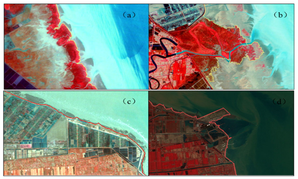
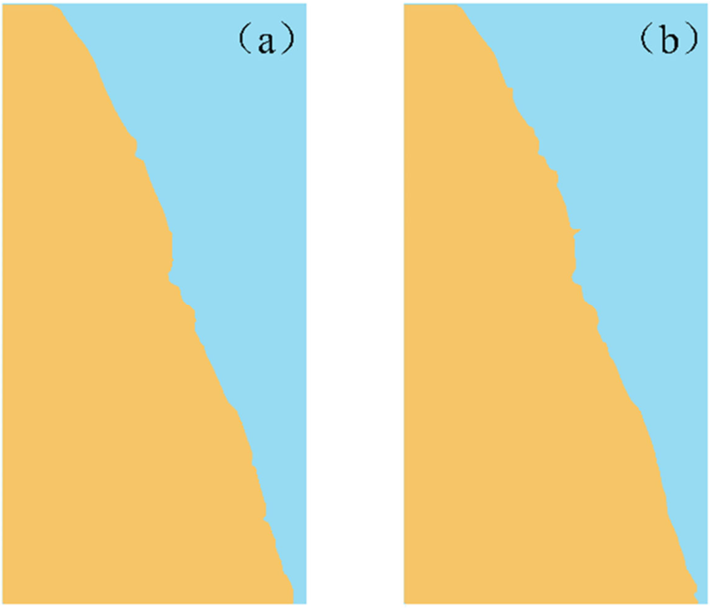
Accurately extracting coastlines requires establishing appropriate classification standards for different coastline types, as they exhibit distinct characteristics in Landsat imagery. This study used a human–computer interactive approach to identify the mean high-tide line, which serves as a proxy for the coastline. The main steps include: first, preprocessing the remote sensing images through radiometric calibration, atmospheric correction, and cropping. Next, the processed images are used to compute the water body index, and OTSU auto-thresholding is applied for water-land segmentation. Considering the complexity and significant human interference along the muddy coast of central Jiangsu. The spectral indices thresholding method, combined with manual visual correction, was used to establish interpretation criteria for natural and artificial coastlines, respectively, for coastline extraction in this study. In the false-color composite image, the vegetation within the submerged high-tide line range is relatively sparse and appears light red. The vegetation on the shore side is denser, with numerous salt-tolerant plants distributed, resulting in a dark red color. Consequently, a distinct vegetation boundary formed near the high-tide line, designated as the interpretive marker of the natural coastline of the muddy coast. For the artificial coastline, the boundary is defined by coastal dikes because they consistently lie above the high-tide line. Because the central Jiangsu coast contains both natural muddy shorelines and highly engineered artificial coastlines, a unified geomorphic shoreline indicator is not applicable throughout the entire study area. Therefore, different proxy indicators were selected according to coastline type to represent the landward boundary of regular marine influence. Coastline-type transitions during different periods were identified through visual interpretation of multi-temporal imagery, and the corresponding coastline was adjusted accordingly. 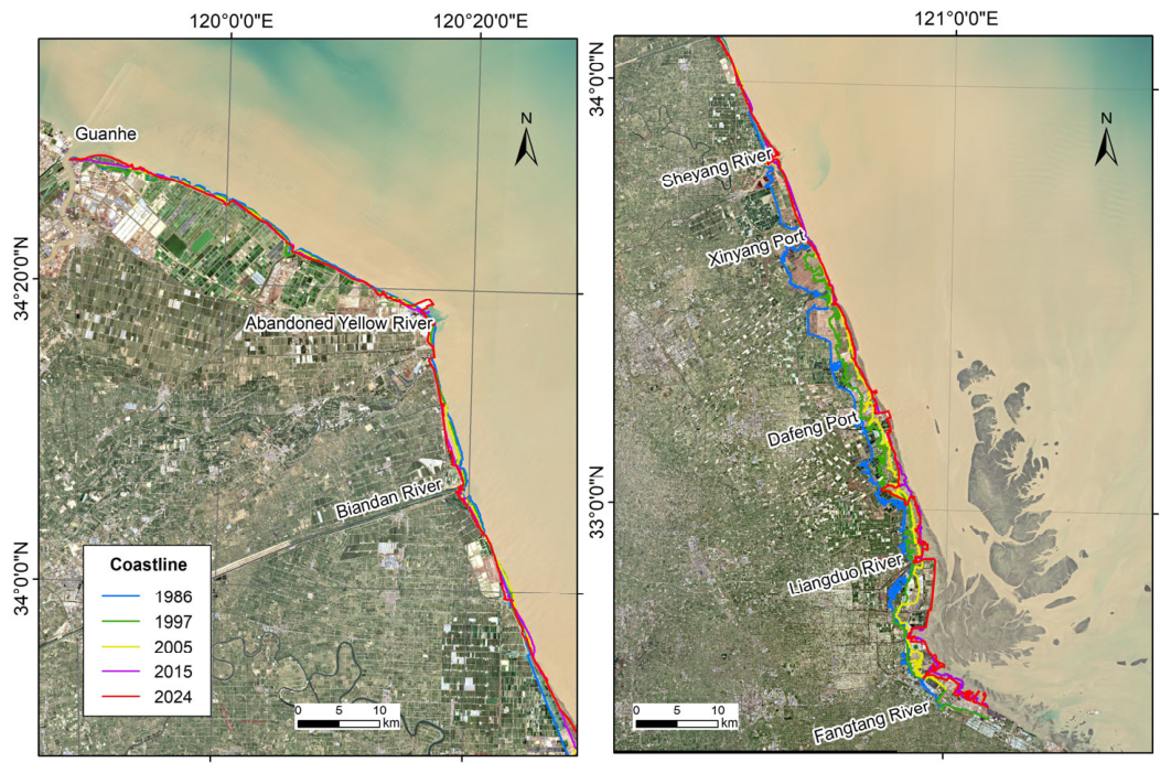Figure 2 demonstrates two types of natural and artificial coastlines along the central coast of Jiangsu Province.

Numerous water indices (e.g., NDWI, MNDWI, AWEI) are widely used for coastline delineation in prior research due to their simplicity and effectiveness. In this study, the Normalized Difference Vegetation Index (NDVI) was used to extract the boundary line of tidal flat vegetation and the Modified Normalized Difference Water Index (MNDWI), which is used to differentiate between land and water, was employed for artificial coastline extraction. It enhances the contrast between land and vegetation, as well as between land and water bodies [40,41]. The formulas for NDVI and MNDWI are as follows:

$$NDVI={\displaystyle \frac{{\rho }_{NIR}-{\rho }_{Red}}{{\rho }_{NIR}+{\rho }_{Red}}}$$

(1)

$$MNDWI={\displaystyle \frac{{\rho }_{Green}-{\rho }_{SWIR}}{{\rho }_{Green}+{\rho }_{SWIR}}}$$

(2)

In Equation (1), the NIR and Red bands correspond to Band 4 and Band 3 in Landsat 5 TM data, Band 5 and Band 4 in Landsat 8 OLI data, and Band 8 and Band 4 in Sentinel-2 MSI data, respectively. In Equation (2), the Green and SWIR bands correspond to Band 2 and Band 5 in Landsat 5 TM data, Band 3 and Band 6 in Landsat 8 OLI data, and Band 3 and Band 11 in Sentinel-2 MSI data, respectively.

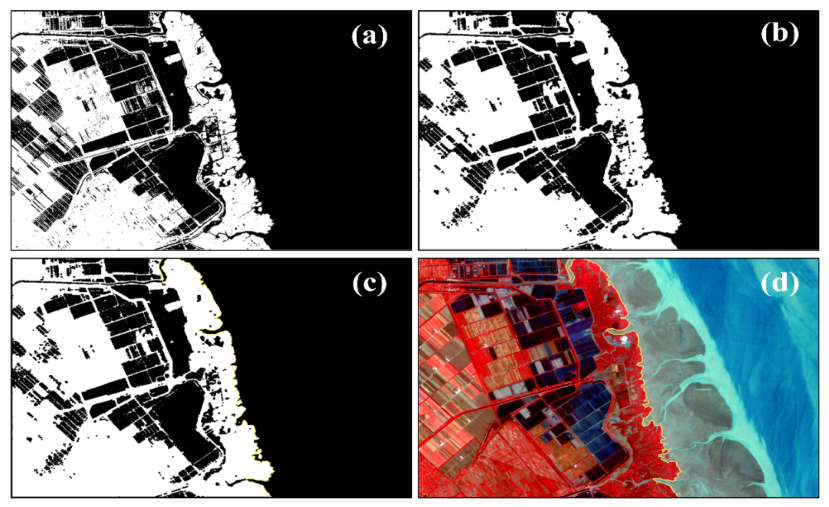
To ensure consistent and reproducible thresholding across all images, the Otsu automatic thresholding algorithm was applied separately to each NDVI and MNDWI image, generating a binary water–land mask without user-defined cutoff values. In the ENVI 6.1 platform, the extracted vegetation and water body pixels are converted into binary raster images, and the close operation in the binary morphology filter function is used to effectively fill the holes in the raster images, remove noise, and smooth the image edges. All morphological operations used a fixed 3 × 3 pixel kernel to maintain uniformity across the entire 38-year time series. Using the ArcGIS platform, raster images are converted to vector coastlines and superimposed on remote-sensing images. The coastline is manually corrected, and accurate coastline information is obtained, as shown in Figure 3.

To verify the accuracy of the extraction, the accuracy assessment method by Hu and Wang (2022) [42] was employed. An independent validation dataset was created by randomly selecting 100 points along the 2020 coastline, visually interpreted from high-resolution Google Earth imagery (0.5 m resolution) as the reference. The RMSE between our extracted coastline and the reference was calculated to be ±15.6 m, indicating acceptable accuracy for Landsat-scale analysis.

The total positional uncertainty of the extracted coastline originates from four main sources: (1) tidal residual (±0.3 m water level variation on a 0.003 slope gives up to ±100 m absolute horizontal displacement, but relative inter-annual uncertainty is only ~±17 m due to consistent MLWS selection); (2) georeferencing error (<0.2 pixels, ~6 m); (3) Landsat pixel resolution (30 m, contributing ~±15 m, consistent with the validation RMSE of ±15.6 m); and (4) manual correction subjectivity (negligible due to strict protocol and 98.5% inter-analyst agreement). The absolute uncertainty (~±101 m) is large, but the relative uncertainty (~±17 m) is the appropriate metric for change detection. Therefore, short-term (5-year) change rates below ~20 m/yr should be interpreted cautiously, while multi-decadal changes (e.g., >100 m) are statistically robust.

2.4. Coastline Change Analysis

The Digital Shoreline Analysis System (DSAS), developed by the United States Geological Survey (USGS), was used to quantify the coastline change rate and provides several statistical methods. Among them, the End Point Rate (EPR) calculates coastline displacement rates using a minimum of two delineated coastlines and a hypothetical baseline. Constructed parallel to the coastlines within the offshore transition zone, this baseline enables quantification of spatiotemporal coastline fluctuations [43].

DSAS v5.0 version is an extension module of the ArcGIS platform, mainly including four core modules: (1) Extracting coastline information; (2) Drawing baselines; (3) Generating equidistant sections; (4) Calculating the rate of coastline change. DSAS can automatically calculate the coastline change rate index in each period by calculating the distance between the coastline and the baseline. Therefore, the appropriate baseline setting is directly related to the accuracy of the change-rate calculation. After numerous attempts and adjustments, five consecutive baselines were drawn along the coast in this study. A total of 1327 orthogonal sections were generated from north to south at intervals of 200 m and with a cross-sectional smoothness of 500. Each cross-section is no more than 8000 m in length and has exactly one intersection point with the coastline of each year.

In accordance with the research requirements, the EPR for each time period was calculated. The calculation formula is as follows:

$$\mathrm{EPR}={\displaystyle \frac{\Delta S}{\Delta t}}={\displaystyle \frac{S_{i+1}-S_i}{t_{i+1}-t_i}}$$

(3)

In the formula, S_i+1 and S_i respectively refer to the distances from the latest and earlier periods of the two consecutive coastlines on the cross-section to the baseline. t_i+1 and t_i represent the imaging dates of the remote sensing images corresponding to the two coastlines. 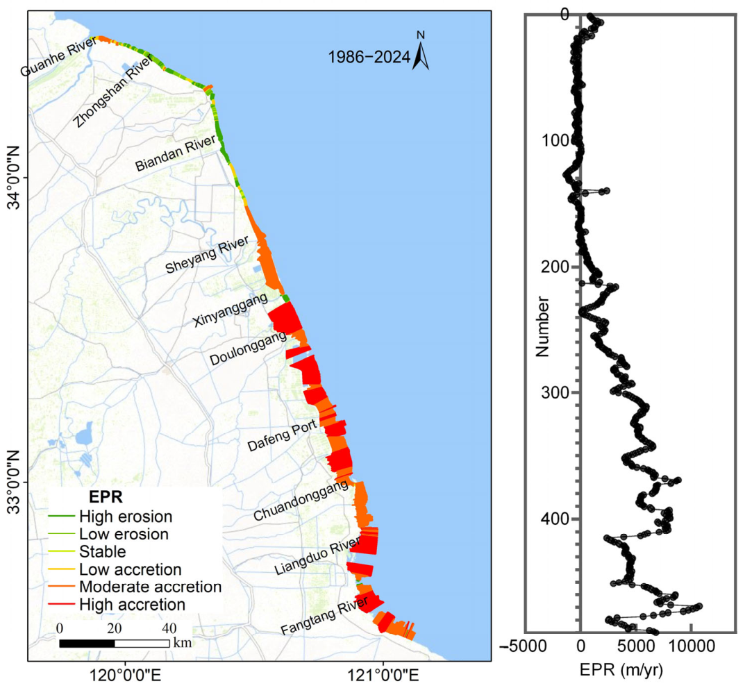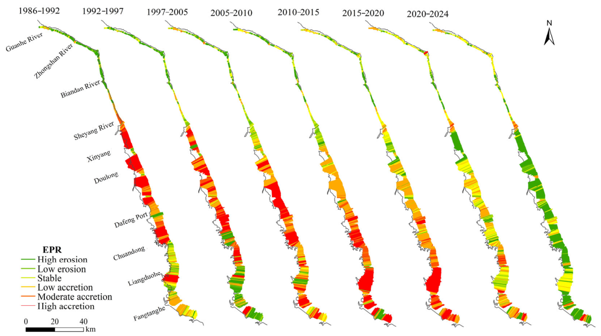In addition, to facilitate the description of the evolution process of the coastline, this study referred to the work of [44], and classified the changing states of the coastline into six categories according to the EPR.

2.5. Clustering of Coastline Evolution Patterns

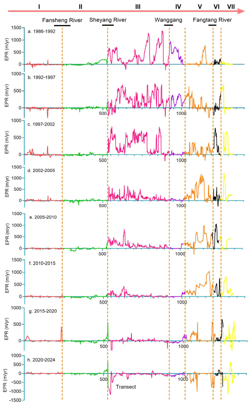
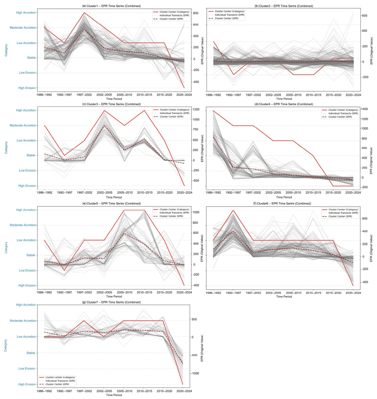
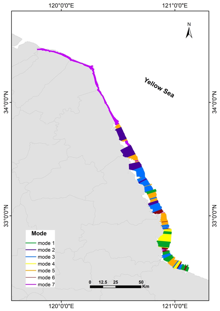
The central coastline of Jiangsu has undergone complex evolution over the past four decades, with significant differences in the evolution patterns of different coastline segments. To explore these distinct evolutionary mechanisms, the K-means clustering method was employed in this study to classify patterns of coastline dynamics. Compared with analyzing coastline change rates within isolated time intervals, cluster analysis of multi-period change-rate data can reveal distinct evolutionary patterns of the coastline and the state transitions between erosion and accretion within each mode.

The K-means clustering algorithm is a commonly used unsupervised machine learning algorithm. Its principle is to divide all the data points in the dataset into a pre-set K cluster, and to make the data points within the same cluster as similar as possible, while the data points between different clusters as different as possible. The K-means algorithm is simple in principle, highly efficient computationally, and is often used to explore potential patterns in data. The K-means clustering was implemented using Euclidean distance with 100 random initializations to reduce sensitivity to local optima, and the final clustering solution corresponded to the minimum within-cluster sum of squares. This study uses the multi-period EPR value sequence for 1327 sections as input data. The coastline change process of each section can be represented as an 8-dimensional vector, such as:

$$x_i=({\mathrm{EPR}}_{i,1},{\mathrm{EPR}}_{i,2},\dots ,{\mathrm{EPR}}_{i,8})$$

(4)

In the formula, x_i represents the coastline change rate vector of the i-th section (i = 1,2, …) (1327), and EPR_i,j represents the EPR value of the i-th section in the j-th period. The input EPR vectors were not normalized because the absolute magnitude of the coastline change rate is an essential characteristic for distinguishing the seven evolution patterns. Normalization would remove differences in change intensity (e.g., −100 m/yr vs. +2 m/yr), potentially merging sections with similar temporal trends but vastly different geomorphic behaviors. Since all EPR values share the same physical dimension (m/yr) and our objective includes classifying by change intensity, the original scale was retained. The K-means algorithm can automatically classify and merge sets of sections with similar temporal evolution patterns. Meanwhile, since the sections are divided at equal intervals, the classification results of the corresponding sections can also be extended to the larger spatial scale of the coastline section.

This study demonstrates the trends of the elbow method and silhouette coefficient for the K-means algorithm. The elbow method metric decreases gradually after k = 4, without a clear “elbow” point forming. Meanwhile, the silhouette coefficient’s increase slows significantly after k = 7, reaching its peak at k = 10, though the differences between values for k = 7 to 10 are minor. Based on these metrics and the interpretability of the classification results, we chose k = 7 as the optimal number of clusters.

2.6. Coastline Change Prediction

A data-driven machine learning method was selected in this study to explore the feasibility of short-term coastline morphology forecasting using a time-series dataset of historical coastlines. In previous studies, predictions were usually based on the cross-section method. However, we aim to directly predict the coastline’s spatial morphology, which is more intuitive and effective than predicting the rate of change of the cross-sectional coastline. Therefore, the Random Forest (RF) model and the convolutional Long Short-Term Memory (Conv LSTM) model were used to capture this temporal variation feature.

Both the RF model and the Conv LSTM model can process time-series data and predict short-term pixel values from raster pixel values. However, the RF model has limitations: it focuses solely on individual pixel variations, neglecting spatial dependencies among adjacent pixels during forecasting. In contrast, the ConvLSTM architecture compensates for this deficiency in learning spatial relationships through integrated convolutional neural network (CNN) modules. Consequently, the RF model is employed as a benchmark to assess the feasibility of traditional machine learning algorithms for short-term foreshore morphological prediction at the pixel level. Comparative analysis with the ConvLSTM model will further assess the potential superiority of deep learning approaches.

The prediction workflow comprises several key steps: First, the RF and ConvLSTM models were trained on the prepared time-series dataset to learn the temporal and spatial patterns of coastline change. Second, the models’ performance was validated by comparing predicted pixel values for 2024 with actual pixel values, thereby ensuring robust predictions. Finally, the optimal model was used to forecast short-term coastline morphology for 2025 and 2030.

2.7. Evaluating Coastline Prediction Accuracy

This study uses the Root Mean Square Error (RMSE) as a statistical metric to evaluate the model’s accuracy, which quantifies the average positional error between the predicted and actual values. In this study, the distance from the coastline to the baseline (2024) is considered the actual value, while the distances to the baseline (2025 and 2030) are considered the predicted values. The formula for calculating RMSE is:

$$RMSE=\sqrt{{\displaystyle \frac{\sum {(x-y)}^2}{N}}}$$

(5)

Here, x is the distance from baseline (Actual year), y is the distance from baseline (Forecasted year), and N is the number of observations.

3. Results

3.1. The Characteristics of Coastline Length Changes

Using satellite imagery, we extracted the characteristics of the spatiotemporal distribution of the study area coastline in five particular stages from 1986 to 2024 as shown in Figure 4. The coastline shows an obvious change in the central coast of Jiangsu during the past 38 years. The coastline in the northern part from Guanhe to the Sheyang Estuary was relatively tortuous, while the coastline in the southern part of the Sheyang Estuary was relatively straight from 1986 to 2024. In addition, we found that the northern part of the Sheyang Estuary experiences relatively slow coastal change, predominantly characterized by retreat from the sea toward the land. However, the coastline has advanced significantly towards the sea in the southern part of the Sheyang Estuary over the past 38 years, particularly during 1986–1997 and 1997–2005. Since 2005, the rate of coastline progradation seaward has decreased significantly.

The length of the coastline in the central region of Jiangsu Province from 1986 to 2024 is shown in Figure 5a. The results indicate that the coastline length in central Jiangsu has declined overall from 1986 to 2024, decreasing from 578.3 km in 1986 to 415.5 km in 2024, with an average annual reduction of 4.28 km. Specifically, the length of the central Jiangsu coastline exhibits an overall pattern of initial decline followed by later recovery and growth. From 1986 to 1988, the length of the central Jiangsu coastline reached its maximum, after which it steadily decreased, reaching a minimum of 365.2 km in 2015. After 2015, the coastline length showed an increasing trend. Although there were fluctuations during this period, the overall coastline length showed significant growth. Between 2015 and 2017, the coastline length rose rapidly, increasing by 63.96 km. By 2023, the coastline length reached the highest value in nearly a decade, at 445.47 km. In 2024, the coastline length slightly declined, but the change was minimal.

The intensity of coastline change in central Jiangsu from 1986 to 2024 is shown in Figure 5b. The results indicate an average change of −0.31%, with fluctuations in both decreases and increases. During the study period, from 1986 to 2015, there was an overall negative growth, with an average negative growth value of −1.5%, along with two troughs. After 2015, the trend was generally positive, with two peaks in growth occurring from 2015 to 2018 and 2021 to 2023, with increases of 8.8% and 5.2%, respectively, although there were two troughs in 2018 and 2024.

3.2. Spatiotemporal Variations of the Coastline

3.2.1. Long-Term Coastline Changes

The DSAS tool was used to quantify coastline changes in coastal evolution from historical coastline positions between 1986 and 2024; endpoint change-rate values for 1326 sections were obtained. After grading the endpoint change rate and visualizing it in ArcGIS 10.5, the calculation results are shown in Figure 6. The long-term coastline change analysis in the central coastal of Jiangsu Province for the 1986–2024 period shows an accretion trend overall, with 66.28% (274 km) of the coastline (879 sections) showing recorded accretion, which includes 2.56% of the rapid accretion, 23.83% of the moderate accretion, and 39.89% of the slow accretion. In addition, 6.86% (28.5 km) of the coastline (91 sections) illustrated stability, whereas 26.85% (111.4 km) of the coastline (356 sections) depicted erosion, including 22.55% of the rapid erosion and 4.3% of the slow erosion.

Spatially, the central coastline of Jiangsu exhibits an obvious difference in accretion and erosion patterns north and south of the Sheyang estuary. With the exception of slow accretion near the Guanhe RiverEstuary and Binhai Port, most of the coastline is dominated by rapid erosion north of the Sheyang River Estuary. However, the coastline is predominantly accreting, with continuous progradation south of the Sheyang Estuary; accretion is most pronounced from Xinyanggang to Wanggang, and from Liangduohe to Fangtang Estuary, with an average accretion of 5 km, and an annual average of 0.13 km per year.

3.2.2. Short-Term Coastline Changes

The short-term results of coastline change from 1986 to 2024 are shown in Figure A1 and Figure 7. The pattern of short-term coastline changes in the study area still exhibits the dynamic pattern of “erosion in the north and accretion in the south”, consistent with the coastline change pattern throughout the study period from 1986 to 2024. However, coastline change rates vary significantly across regions and time periods, with repeated shifts between erosion and accretion. Thus, the period from 1986 to 2024 was divided into eight consecutive five-year intervals to analyze the dynamic characteristics of coastline change in the study area.

Zone I exhibited pronounced erosional trends during the 1986–1992 and 1992–1997 periods, with average coastline change rates of −11.8 m and −18.5 m, respectively. Meanwhile, the average erosion rates were −19.9 m and −22.9 m. However, the coastline as a whole exhibited a stable trend after 1997, attributable to the implementation of coastal protection projects and the construction of coastal ports.

Zone II extends from the Fanshen Estuary to the Sheyang Estuary; the coastline exhibited overall fluctuations and stability prior to 2002, after which it showed a pronounced erosional trend. Especially during the period from 2005 to 2010, obvious erosion has occurred in the area north of the Shuangyang Estuary; the percentage of transects depicting erosion (69.23%) was higher than those depicting accretion trends, with the average coastline change rate of −15 m, and the maximum erosion rate reaching 119 m. However, the erosion trend in this area has gradually eased over the past two periods and has entered a stable, changing state, primarily due to the construction of the artificial sea dike project. In addition, obvious erosion has occurred from the Shuangyang Estuary to the Yunliang Estuary since 2015, and the erosion has shown a significant strengthening trend.

Zone III exhibited the highest accretion trend with 96% of transects, and the entire coastline has advanced towards the sea over the past 38 years. The coastline underwent multiple state transitions around the Sheyang River during the study period, progressing from accretion (1986–1992) to rapid accretion (1992–2002) and then to slow accretion (2002–2024). Prior to 2010, the coastline segment between the Sheyang Estuary and Wanggang coast was characterized by overall progradation. The most rapid accretion phase occurred from 1986 to 2002, with an average offshore advance of 350 m during 1986–1992. Since 2010, coastal accretion has significantly decreased, and erosion has occurred in some sections of the coastline. During 2015–2020, the percentage of transects indicating erosion (30%) was higher than before 2015. The 2020–2024 period observed the highest percentage of transects under erosion (83%) of all the periods under observation.

Zone IV showed the highest progradation trend before 2015, with all of the transects exhibiting accretion characteristics. However, the coastline has shifted from accretion to erosion in recent years.

Zone V–VII exhibited an overall accretionary trend of the coastline throughout the entire study period. However, the accretion rate continues to decline, and erosion has occurred in some sections of the coastline. This is mainly due to the complex coastal dynamics in this area, which are influenced by fluctuations in tidal creeks.

3.2.3. Coastline Evolution Model

To better understand the dynamic changes along the central coast of Jiangsu Province, we employed K-means clustering to classify the erosion and deposition processes across different coastal sections. Based on a dataset of eight periods of coastline endpoint change rates from the previous research area, we clustered 1326 sections into seven groups with distinct change patterns. The spatial distribution of their evolution patterns is shown in Figure A2. There are significant spatial distribution patterns among the different coastline evolution patterns, with patterns 1–4 showing a relatively concentrated spatial distribution, while patterns 5–7 are scattered across the entire coastal section. Among them, the section of pattern 2 covers the continuous coastline from the Guanhe Estuary to the Sheyang estuary, totaling 581 sections, which is the most widely distributed and concentrated coastline evolution pattern. Apart from the differences in spatial distribution continuity, the distribution patterns of different pattern sections are also different. Patterns 2 and 4 are mainly concentrated in the north and central parts of the research area, while patterns 3, 5, and 7 are only distributed in the south. Patterns 1 and 6 appear in the central and southern parts, respectively. The north–south differences and the concentrated or interlaced distribution patterns of these different pattern sections reflect differences in natural geographic conditions and hotspots of human activity.

Mode 1: Accretion

To further analyze the specific dynamic processes of each evolution mode, we examined the conversion between the corresponding coastline erosion and accretion states for each mode. The clustering results of the cross-sections for Evolution Mode 1 are shown in Figure 8a. The results indicate that this section is mainly located in parts of Dafeng Port and Tiaozini. From 1986 to 2024, it exhibited overall accretion, but the accretion rate declined over time. From 1997 to 2002, it exhibited rapid accretion. Subsequently, the coastline change began to slow down and gradually became a slow accretion. Especially since 2020, the coastline has tended to stabilize, and some sections of the coastline have even begun to experience erosion. Compared with remote sensing images, it was found that during 1997–2002, these sections experienced frequent human activities, the area of tidal flats increased substantially, and the coastline migrated rapidly towards the sea. In subsequent periods, the spatial development of the coastal tidal flats continued at a certain pace, while the coastline migrated towards the sea at a slower rate. However, in the recent 2020–2024 period, the coastline development began to slow down or even stop. In some southern sections of the Mode 1 coastline, enhanced water flow eroded the front edge of the tidal flat vegetation adjacent to the coast, resulting in coastline retreat.

Mode 2: Rapid transition between erosion and accretion

The results of the section clustering in the Evolution Mode 2 show that the main distribution is in the section from the Guanhe Estuary to the Shiyang estuary (Figure 8b). During the study period, the coastline was relatively stable overall, but there were multiple transitions between erosion and accretion states. Especially from 1992 to 1997 and from 2005 to 2015, there were more obvious erosions. By comparing the initial and final states of the coastline during the entire study period, most of the sections except for the parts south of Guanhe Estuary and north of Shiyang estuary, and the port and wharf, showed significant erosion changes. The distribution area of the section in Mode 2 consists mainly of muddy natural and artificial coastlines. The artificial coastlines comprise large areas of artificially filled fish ponds and salt fields, which are key development areas in the marine coastal zone economy. However, the muddy tidal flats and unprotected fish ponds in this area are sensitive to environmental change and prone to erosion under natural forces such as waves and storm surges. To prevent coastal erosion, artificial seawalls were installed in this section. In addition, more stable artificial structures, such as port docks, were less susceptible to disturbances. The erosion–accretion changes in the section in Mode 2 were overall stable under the joint control of human and natural factors, but the coastline underwent multiple transitions due to shifts in dominant factors over time.

Mode 3: Moderate accretion—accelerated accretion—decelerated accretion

The results of the section clustering in Mode 3 are shown in Figure 8c, indicating that the main distribution is in the section between the 1125th and 1156th sections and the 1268th and 1280th sections. The distribution area is adjacent to the Tiaozini area. During the entire study period, it exhibited an overall accretion-change state, with the fastest accretion rates from 2002 to 2005 and from 2010 to 2015, followed by a decrease in the accretion rate, which has been relatively stable since 2020. The slope of Tiaozini is gentle, and the width is large, which is one of the typical muddy tidal flats in the world. Due to the superior geographical conditions and the demand for the development of the coastal intertidal zone space in this area, large-scale tidal flat reclamation projects were carried out in the corresponding section of Mode 3. Under the guidance of the “Regulations on the Use of Sea Areas of Jiangsu Province”, tidal flat reclamation intensified from 2002 to 2015, transforming the coastline from natural to artificial and advancing toward the sea at an accelerated rate.

Mode 4: Rapid accretion—relative stability

The results of the section clustering in Mode 4 are concentrated in the section south of the Sheyang estuary to the Doudonggang area, as shown in Figure 8d. The dynamic characteristics of the coastline change in this mode are significant. Before 1992–1997, it was in a rapid accretion state, with an endpoint change rate exceeding 400 m per year, and the coastline change amplitude was pronounced. Then the coastline began to erode, especially since 2020, and the erosion intensity has further increased. These sections are mainly located within the buffer zone of the Nature Reserve in Yancheng City, with a majority of natural coastlines. With the reduction of erosion materials in the north of Jiangsu Province’s abandoned Yellow River delta and the enhancement of water dynamics, coastal erosion has further intensified.

Mode 5: Accelerate accretion–decelerate accretion

The results of the section clustering in Mode 5 are shown in Figure 8e. The change rate of the coastline shows a trend of first accelerating and then decreasing. The change rate of the coastline during the 1986–2002 period was relatively low, distributed between slow erosion and slow accretion, and then the accretion change rate began to accelerate, especially during the 2005–2015 period, reaching the peak of accretion speed, and then the accretion speed decreased significantly and tended to stabilize. The distribution area of Mode 5 from north to south includes Dafeng Port, and the Tiaozini, Lao Bagang, and Xiaoyangkou areas. The results of remote sensing image interpretation show that these sections are all typical artificial coastlines, such as embankments and port docks. Take Dafeng Port as an example. The construction project of Dafeng Port began in 1988 and the first phase was completed in 2005. The second-phase expansion project was completed between 2005 and 2020.

Mode 6: Accelerated accretion—slow accretion—erosion

The clustering results for Mode 6 are shown in Figure 8f. The evolution of the coastline exhibits a “first acceleration—then flattening—and finally deceleration” transformation. Coastline change was accelerated in the early stage, peaking in accretion during 1992–1997, then it decelerated and entered a long-term, slow accretion state. Since 2015, it has begun to stabilize or turn into erosion. Unlike Mode 1, the evolution of this mode was relatively stable during the middle stage, with a small amplitude of change, and it essentially remained in the slow accretion state. The distribution of the coastal segments of Mode 6 is relatively scattered and interspersed across the central and southern parts of the study area, predominantly consisting of small ports and artificial coastlines near estuaries. The construction scale of these coastal segments is smaller than that of the ports in Mode 5, and the horizontal expansion scale in the direction of the sea is also relatively smaller. For example, the embankment project in the south of Dafeng Port did not build port docks extending towards the sea. Therefore, the mid-term state of coastline change for these coastal segments is characterized by slow accretion.

Mode 7: Accretion—Rapid erosion

The clustering results of Mode 7 are shown in Figure 8g. The early stage of the coastal segments of Mode 7 was mainly slow—moderate accretion, with fluctuations in the accretion rate, but the overall accretion trend did not change. However, after 2015–2020, the coastline change suddenly shifted to rapid erosion. Mode 7 is one of the modes with the fewest number of cross-section clusters, containing only 65 cross-sections. The distribution of the coastal segments of Mode 7 is concentrated in the south of Chuandonggang, Dongtai Estuary, Liang Dao Estuary, and Fang Tang Estuary. The removal of salt marshes may have reduced the muddy coast’s ability to capture suspended sediment, resulting in short-term coastal erosion.

4. Discussion

4.1. Exploratory Coastline Evolution Forecasting

To deeply explore the evolutionary patterns of the central coast of Jiangsu Province, this study, based on historical change analysis, further employed machine-learning methods to predict the short-term evolution of the coastline. Machine learning offers a new data-driven approach to capturing dynamic changes in recent coastal data. This section presents the coastline predictions for the study area using the random forest and convolutional long short-term memory model developed in Section 2.6 and evaluates their validity through overlay comparisons and model evaluation metrics. It should be noted that the forecasting analysis presented in this study is exploratory in nature and primarily aims to evaluate the feasibility of applying RF and ConvLSTM models to long-term coastline evolution datasets with sparse temporal observations.

For the random forest model, based on the binary-processed 2024-year prediction grid, the overall accuracy rate is 0.97, and the pixel accuracy rate is 0.95 (Figure A3a). However, because 72.7% of pixels in the study area did not change across the historical sequence, the overall accuracy overestimates the model’s performance in the changing area. Therefore, this study also calculated the pixel accuracy within the historical change pixel area, which decreased to 0.87, indicating that the model’s predictive ability for dynamic changes is limited. Further comparison of its 2025-year prediction results (Figure A3b) revealed that pixels with state changes between consecutive years accounted for only 0.0223%, well below the reasonable expectation. This indicates that although the random forest model achieves apparent high accuracy, its predictions are overly dependent on the pixel sequence, and it is unable to effectively capture complex spatiotemporal change patterns. Therefore, it is not suitable for the coastline prediction task of this study.

In contrast, the ConvLSTM model, as a regression model, can be evaluated by the root mean square error. The best ConvLSTM model in this study has an RMSE of 0.13, indicating a good fit. To conduct a fair comparison with the random forest, its classification metrics were also calculated: the overall accuracy of the binary-processed 2024-year prediction grid is 0.98, and the pixel accuracy is 0.98 (Figure A4). In the historical change area, the overall and pixel accuracies remained 0.94 and 0.94, respectively, indicating a slight decline in performance, demonstrating that the model can effectively learn the spatiotemporal dynamics of the changing area. A comprehensive comparison shows that, in handling long-term sequences with complex spatial features, the ConvLSTM model demonstrates substantially superior predictive performance compared with the random forest model and can effectively learn spatiotemporal dynamics in pixels.

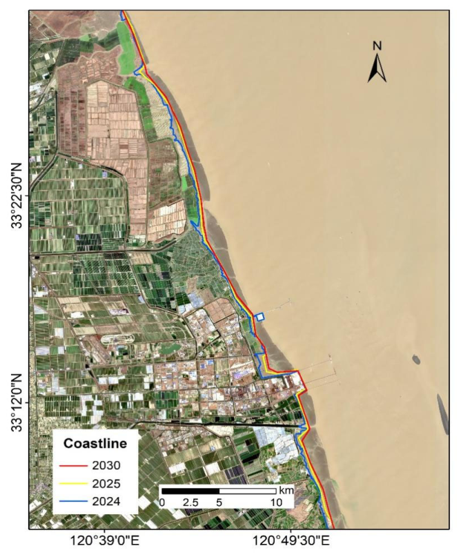
This study employs a more performance-optimized ConvLSTM model to predict short-term coastline form, projecting coastline form for the experimental area through 2030. The prediction results show that, compared with the 2024-year coastline, the 2025-year and 2030-year coastlines generally exhibit seaward accretion (Figure 9). The future coastline change rate calculated using the digital coastline analysis system further indicates that the coast of the study area will mainly undergo slow accretion in the future. This trend is consistent with the classification conclusion for the evolution mode of Doulonggang in Section 4.3: “early rapid accretion—continuous deceleration”. Therefore, the forecasting results should be interpreted as exploratory trend scenarios rather than deterministic future coastline positions.

4.2. Driving Forces of Coastal Change

Sediment load, sea-level change, local hydrodynamics, and artificial reclamation play important roles in the long-term evolution of the coastline, whose accretion–erosion dynamics are governed by the coupling between sediment input and local sediment-trapping capacity [10,45]. Sources of sedimentary material significantly influence changes in erosion and deposition along the Jiangsu coast. In 1128, the Yellow River diverted to the Huai River and entered the Yellow Sea off the northern Jiangsu coast, carrying a large amount of sediment that accumulated there, causing the northern Jiangsu coast to rapidly advance seaward. In 1855, as the Yellow River shifted northward and changed course to flow into the sea via Shandong, sediment transport from the Yellow River to the southern Yellow Sea almost ceased. This likely contributed to a relative increase in ocean dynamics, and the Jiangsu coast entered a new adjustment phase, primarily characterized by erosion of the abandoned Yellow River delta, retreat and leveling of adjacent coastal sections, and further accretion of the southern coast. To ensure the safety of seawalls and halt erosion, the state has constructed an 11.2 km-long seawall revetment project since 1967. The entire 1.594 km section of the Liuhezhuang seawall was constructed with a dry-laid stone revetment to initially control coastal erosion. Jiangsu Province has undertaken several seawall improvement projects since 1997, further strengthening its coastal protection system. Research shows that over the past 38 years, the abandoned Yellow River delta area has remained a rapidly eroding section. However, due to the protection of coastal dikes, the coastline has been relatively stable since 2015. Furthermore, with the southward shift of the Yangtze River estuary and the reduction of sediment entering the sea, especially with the construction of the Three Gorges Dam, the amount of sediment entering the sea from the Yangtze River has decreased from 500 million tons in the 1950s to 124 million tons since 2003 [46], leading to a further reduction in the amount of material transported from the Yangtze River to the Jiangsu coast. Temporally, this reduction coincides with a marked slowdown in accretion rates along the southern central Jiangsu coast (from approximately 350 m per year prior to 2005 to approximately 50 m per year following 2015), indicating a potential causal relationship. However, establishing a direct causal link is complicated by concurrent changes in reclamation policy and local hydrodynamics. While reduced sediment supply is a plausible contributing factor, quantitative attribution would require numerical modeling (e.g., sediment budget or coupled wave–current–sediment transport models). Over the past few decades, the sea level in Jiangsu has been rising at a faster rate than the national average. This trend, combined with the reduction in sediment flowing into the sea and the subsidence of the land, is reshaping the coastline of Jiangsu.

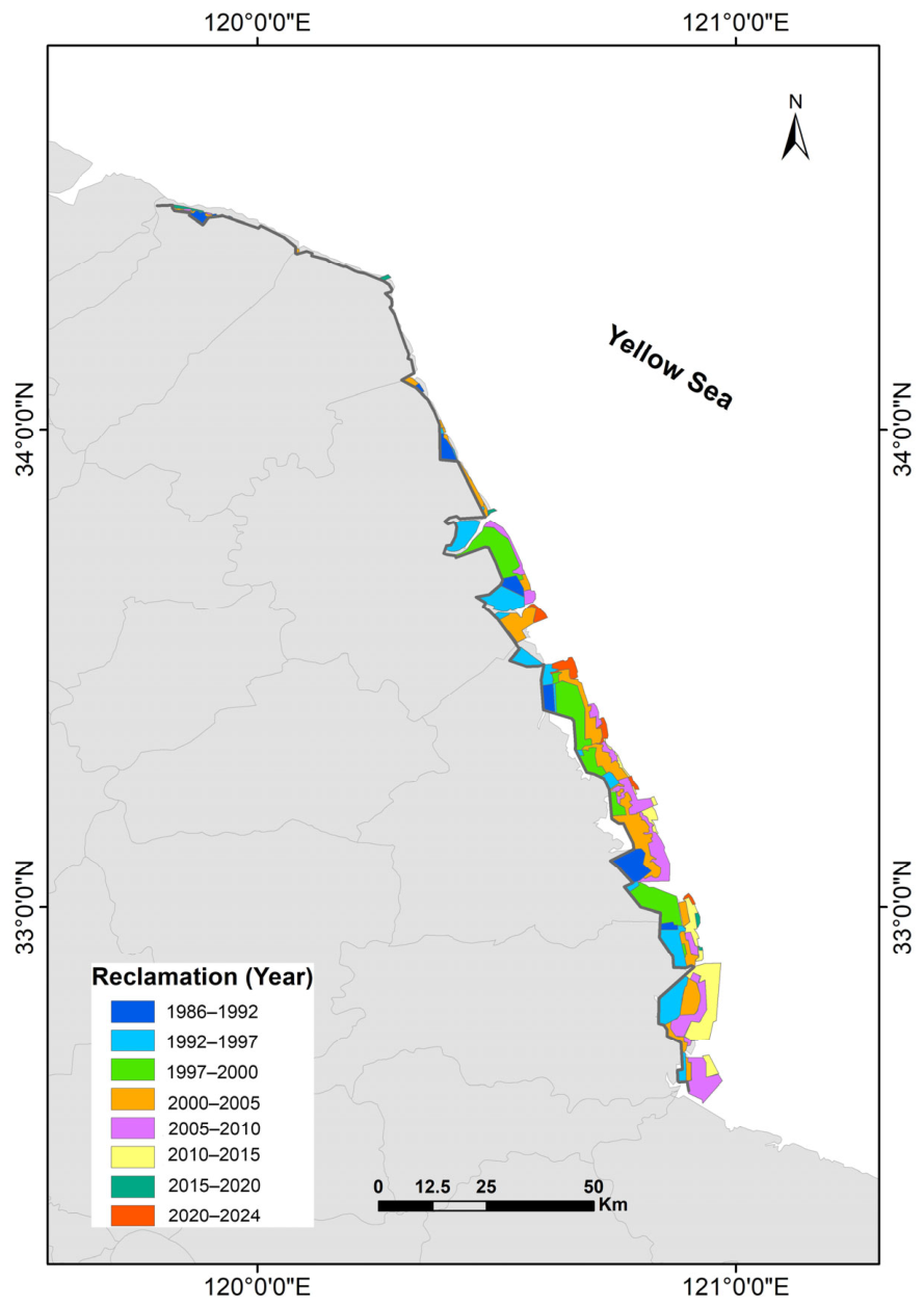
Coastal reclamation projects are a major way for Jiangsu Province to alleviate the conflict between population and land use. Historically, the coastal reclamation area in Jiangsu Province reached 200 × 10⁴ hm² (Jiangsu Provincial Agricultural Resources Development Bureau, 1999). Since 1949, large-scale coastal reclamation in Jiangsu has been the primary driver of the rapid coastline expansion. It is evident that large-scale coastal reclamation can significantly alter the coastline, extending it from land to ocean and reshaping its geometric morphology. In this study, we combined Landsat data to conduct statistics on coastal reclamation in central Jiangsu (Figure 10). It can be seen that in the past few decades, coastal reclamation in central Jiangsu has expanded significantly, with a total reclaimed area of 10.07 × 10⁴ hm² and an average annual expansion of 0.27 × 10⁴ hm². Meanwhile, the temporal changes in reclamation along the central coast of Jiangsu Province from 1986 to 2024 were statistically analyzed. The results indicate that the reclamation area along the central coast of Jiangsu Province increased first and then declined from 1986 to 2024. The largest increase occurred between 2000 and 2005, reaching 22,234 hm². 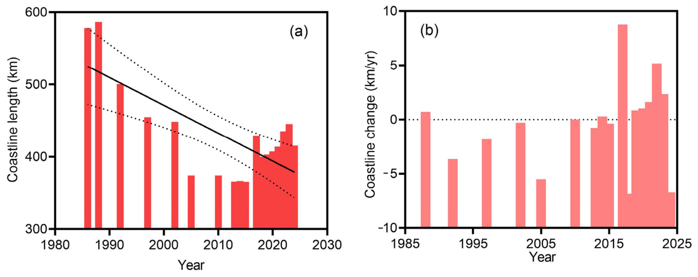The reclamation growth rate before 2000 was 3346 hm²/yr, while the growth rate after 2000 was 2243 hm²/yr. This further suggests that, in the evolution of the Jiangsu coastline, the overall coastline has been relatively stable since 2020, with some sections exhibiting pronounced erosion. The reasons for this phenomenon are mainly related to national policy regulation. The “aquaculture-oriented fisheries policy” implemented in Jiangsu in the 1980s, the “Maritime Development of Eastern Jiangsu” in 1995, and the national strategy to develop the Jiangsu coast in 2009 all promoted the continued expansion of coastal reclamation [34]. After 2010, with the release of the Jiangsu Provincial Coastal Tidal Flat Reclamation and Development Plan, the growth of reclamation in Jiangsu slowed significantly [47]. In 2017, the State Oceanic Administration adopted the ecological construction guidelines for land reclamation projects, emphasizing the importance of ecology. In particular, in 2018, the State Council issued a notice on strengthening the protection of coastal wetlands and strictly controlling land reclamation, strictly controlling new land reclamation and strengthening marine ecological protection and restoration, resulting in relatively stable coastlines. Changes in sedimentary dynamics are an important factor in the evolution of coastal tidal flat landforms [48]. Since 1855, the Jiangsu coast has entered a new phase of adjustment. The impact of Yellow River runoff on the coast has gradually weakened, whereas the dominant role of nearshore tidal currents has gradually strengthened, resulting in increased coastal and inland erosion of the abandoned Yellow River delta. Furthermore, the sediment eroded by the abandoned Yellow River is transported southward under the dynamic influence of tidal currents, thus continuing to provide abundant sediment for the seaward advancement of the central Jiangsu coast [48]. However, with the implementation of the coastal erosion protection project along the abandoned Yellow River in northern Jiangsu, the supply of sediment generated by coastal erosion has gradually decreased, leading to the southward expansion of coastal erosion. Furthermore, the Xiyang Channel, an important tidal channel off the coast of central Jiangsu, continues to extend southward under the influence of nearshore hydrodynamics, resulting in ongoing nearshore erosion. Under the influence of ocean currents along the Jiangsu coast, eroded material is constantly transported inland and southward. In the Tiaozini area of central Jiangsu, tidal currents have been moving steadily toward the coast in recent decades, disrupting the erosion–deposition balance of the tidal flat profile and significantly accelerating coastal erosion. In addition, the central Jiangsu coastal area is a strong-tidal coast; when strong currents impact the concave coastline, they cause coastal erosion.

Global warming will accelerate sea-level rise, intensifying storm surges and waves and increasing their frequency, thereby increasing the likelihood of coastal erosion. The average sea-level rise rate in the Jiangsu coastal area is 2.2 mm/yr, making it one of the regions with the most significant relative sea-level rise in China, which will lead to a decline in the seawall defense capacity of the Jiangsu coastal area and a further expansion of the coastal erosion area. However, the magnitude and rate of future sea-level rise remain uncertain, and its interaction with sediment supply and human interventions will determine the net erosion risk.

4.3. Coastal Erosion Risks and Managements

Over the past 38 years, the northern part of the central coastline of Jiangsu Province has shown the characteristic of erosion, and the erosion has shown the characteristic of strengthening towards the south, which faces degradation risks from external forcing and internal geomorphic conditions—firstly, with the depletion of erosion materials in the abandoned Yellow River Delta and the reduction of sediment flowing into the sea from the Yangtze River [49]. If the abandoned Yellow River has been basically flattened since 2000, the erosion range has spread to both sides, the coastal material has coarsened, the characteristics of a sandy coast have emerged near the shore, and the annual riverine sediment discharge has decreased by 70% since the operation of the Three Gorges Dam in 2003 [50]. Secondly, with the sudden interruption of water and sediment inflow from the Yellow River, significant changes have occurred in the dominant coastal dynamic processes. For example, the wave effect was relatively weak during the period of 1128–1855 compared with the fluvial and tidal processes. However, since 1855, wind waves have been more significant for erosion of the coastal area of Jiangsu, as well as for sediment transport in the coastal and tidal flats. Meanwhile, due to the influence of converging and diverging tidal dynamics off the coast of central Jiangsu, the convergence and convergence points of the two coastal tidal waves gradually shift southward, resulting in the continuous enhancement of coastal hydrodynamic forces and the increased sediment-carrying capacity of nearshore tidal currents. Third, climate change-induced sea level rise and intensified typhoon activity pose additional threats to coastline erosion. A recent study from Gong et al. (2019) indicated typhoon waves have a short-duration and interlude erosion effect on the coast, with a coastal scouring volume of 0.2 to 0.4 m, accompanied by significant coastal transport [51]. Such extreme events have the potential to exacerbate coastal erosion, particularly if their frequency or intensity increases under climate change. However, the long-term contribution of typhoons to the multi-decadal erosion trends observed in our study cannot be quantified directly from our data. We therefore note that typhoon-driven erosion represents a plausible additional risk factor, not an established cause of the observed 38-year patterns. This will further threaten coastal stability and precipitate its collapse. In addition, although the construction of coastal protection engineering has to some extent prevented coastal erosion, which has led to the artificial construction of the coastline, the tidal flat profile of the coast continues to steepen. Thus, enhanced coastal dynamics will lead to coastal collapse and damage. Consequently, erosion along the central coast of Jiangsu Province is likely to continue or even intensify in the future, particularly if sediment supply remains low and sea-level rise accelerates. However, the actual trajectory will depend on future human interventions (e.g., reclamation policies, coastal protection engineering) and natural variability.

The impact of coastal erosion on coastal evolution in Jiangsu necessitates integrated management of the coastal ecosystem for long-term sustainability. Coastal salt marshes, acting as natural buffers against storm surges and waves, play a vital role in coastal protection. In the past 50 years, some countries have experienced salt marsh loss rates of 70–80%. In response to the current state of silty coastal erosion in Jiangsu, coastal salt marsh wetland ecological restoration projects can be implemented to restore and enhance coastal ecosystem functions. In areas with strong erosion, a combination of rigid structural protection and flexible ecological beach protection measures can be rationally adopted. Through key coastal engineering construction, the coastline profile and morphology can be balanced and stabilized. For example, a pilot project in the abandoned Yellow River delta using a combination of “artificial headland + offshore submerged breakwater” was conducted. The breakwater was 500 m from the shore with a top elevation of −1.5 m, reducing wave energy by over 30% and promoting an accretion rate of 15 cm/year. Furthermore, scientific measures to promote accretion should be implemented to increase tidal flat resources. Along the Jiuduansha coast of the Yangtze River estuary, ecological restoration through strategic planting of salt-tolerant plants significantly increased intertidal sediment deposition and has therefore been widely adopted [52]. In addition, considering the powerful destructive force of typhoons on coastal erosion, strengthening research on the typhoon response to coastal sediment dynamics and establishing relevant forecasting and early warning systems are crucial [53]. Improving the ability to resist the threat of sea-level rise is also essential for comprehensive tidal flat management. Simultaneously, establishing a three-dimensional monitoring network and an intelligent disaster early warning platform will enhance the high-precision early warning capabilities for coastal erosion disasters.

4.4. Problems and Prospects

This study provides a comprehensive, multi-decade perspective on coastline modifications; however, it is essential to acknowledge several limitations inherent in satellite monitoring within muddy, highly dynamic environments. The use of 30-m Landsat imagery, while appropriate for assessing long-term regional trends, may not detect small-scale morphological changes or short-term oscillations in the intertidal zone that occur within a single pixel. Despite efforts to select images with similar tidal conditions, the 16-day Landsat revisit cycle, combined with frequent cloud cover in coastal China, often limits the availability of ‘perfect’ high-tide scenes. Consequently, these uncertainties may affect the identification of localized short-term coastline oscillations, particularly in areas characterized by highly dynamic tidal-flat morphology. Therefore, the short-term fluctuations observed in some coastal segments should be interpreted with caution. Nevertheless, because this study focuses primarily on long-term, multi-decadal evolution trends derived from consistent time-series observations, the major spatial patterns identified—such as the “erosion in the north and accretion in the south” configuration—remain reliable at the regional scale. Similarly, the clustering-based evolutionary patterns should be regarded as representative regional evolutionary modes that capture dominant temporal behaviors, rather than as precise, deterministic classifications for every local coastline segment.

In addition, this study introduces the K-means clustering algorithm into research on coastline change. Based on quantitative coastline change data obtained from the digital coastline analysis system, the system enables data-driven discovery of coastline evolution patterns and interprets each pattern in terms of regional geographic conditions and human activities. Compared with simply comparing the rate of coastline change across different periods, the results of coastline pattern clustering analysis focus more on the transformation of erosion and accretion states throughout the entire evolutionary process. The explanation of the evolutionary mechanism is insufficiently specific. Previous studies have widely applied Empirical Orthogonal Function (EOF)-based methods to investigate longshore coastline variability and identify dominant modes of coastal evolution. EOF analysis is particularly effective for extracting large-scale spatial-temporal covariance structures and detecting dominant oscillation signals in coastline datasets. Compared with EOF-based approaches, the K-means clustering method adopted in this study focuses more on identifying discrete evolutionary states and transitions between erosion and accretion processes among different coastline segments. Therefore, the two approaches are complementary: EOF methods emphasize dominant continuous variability patterns, whereas clustering analysis is better suited to distinguishing heterogeneous regional evolutionary behaviors and interpreting their relationships with geomorphological conditions and human activities. In the future, it is hoped that more data and indicators, such as the types and densities of tidal flat vegetation, the flow of various rivers flowing into the sea, and the detailed classification of artificial coastline types, can be combined to conduct a more in-depth study of the driving mechanisms in each evolution pattern. In addition, important historical change analysis and future coastline change prediction were carried out on the central Jiangsu coastline. The analysis results and prediction results should be combined with specific coastal spatial management and planning to provide truly effective data support and a theoretical basis. However, the forecasting framework developed in this study is subject to several limitations. First, the temporal training dataset contains only nine coastline snapshots, which may limit the robustness and generalization capability of the deep-learning model. Second, the predicted 2030 coastline should be interpreted as a trend-oriented scenario under recent historical evolution conditions rather than a deterministic future coastline position. Third, model validation was conducted only using the 2024 coastline dataset and relied primarily on pixel-based image similarity metrics rather than direct coastline-position error assessment. Future studies should incorporate denser temporal observations, coastline-distance-based validation metrics, and hydrodynamic forcing variables to improve forecasting reliability.

5. Conclusions

In this study, we analyzed the patterns and trends in the evolution of Jiangsu’s coastline using remote sensing imagery from 1984 to 2024. The main research conclusions are as follows:

(1)

The trend of the length change of the central Jiangsu coastline over the past forty years is that it first continuously shortens and then recovers and grows, but the overall coastline length has decreased significantly. In 2024, the coastline length was reduced by approximately 162.8 km relative to the peak. Throughout the study period, coastline changes were dominated by accretion, exhibiting a spatial pattern of “erosion to the north and accretion to the south”, with the Sheyang estuary as the boundary. For example, most of the coastline from south of the Guanhe estuary to north of the Shuangyang estuary experienced continuous erosion, while areas from Xinyanggang to Wanggang, and from Liangduohe estuary to Fangtanghe estuary, showed significant accretion. Calculations of coastline change rates over multiple periods showed that the erosion and accretion states of each coastline segment underwent multiple transformations during the study period; however, the overall pattern of “more erosion in the north and more accretion in the south” remained consistent.

(2)

The recent evolution of various coastline segments in central Jiangsu can be summarized into seven patterns, reflecting multiple transformations of erosion and accretion states during the evolution of different coastline segments. Among them, the “rapid erosion–accretion transition” pattern is the most widespread, mainly distributed between the mouths of the Guanhe River and the Sheyang River. This pattern primarily involves natural silty coastlines and artificial coastlines dominated by aquaculture ponds and dikes. Under the influence of natural forces such as waves, tidal currents, and storm surges, relatively weak artificial structures are easily damaged, leading to displacement and rapid changes along the coastline. Another pattern, “early-mid-accelerated accretion—late-decelerated accretion,” is mainly distributed near the Tiaozini mudflats. Its evolutionary process closely matches the temporal sequence of coastline advance associated with large-scale mudflat reclamation projects. The spatial distribution of these patterns and the transition process of coastline erosion and accretion in these patterns reflect the complex coupling effect between regional geographical conditions, such as tidal flat vegetation growth, sediment supply, and hydrodynamic conditions, and human activities, such as mudflat reclamation, land reclamation, aquaculture, and salt production, on coastline evolution.

(3)

For predicting short-term (5-year) coastline morphology, the ConvLSTM model achieved an RMSE of 0.13 and an overall accuracy of 0.98 on the 2024 validation data, substantially outperforming the random forest model (overall accuracy 0.97, pixel accuracy in change areas 0.87). Based on the optimal ConvLSTM model, the model results suggest a potential tendency toward slow accretion under recent historical evolution conditions (average rate < 10 m/yr) by 2025 and 2030.

(4)

Sediment supply reduction (e.g., Yangtze River sediment load decreased from ~500 Mt/yr in the 1950s to ~124 Mt/yr post-2003) and human reclamation (accounting for >80% of seaward advance before 2015) are the dominant drivers of coastline changes. Ongoing material depletion, accelerated sea-level rise (2.2 mm/yr locally), and increased frequency of extreme marine storms have heightened the risk of coastal erosion. Therefore, integrated management measures—including ecological restoration of salt marshes, scientific promotion of accretion, and adaptive reclamation policies—should be implemented.