1. Introduction
High-resolution active 3D radar imaging [
1] plays a pivotal role in complex environment sensing and precision remote sensing, with extensive applications in maritime vessel collision avoidance, search and rescue [
2], civilian air traffic control (ATC), and urban air mobility (UAM) management. The fidelity of radar point-cloud reconstruction is highly dependent on the system’s capability for high-precision angular estimation of spatial targets. Theoretically, angular information can be extracted via narrow-beam and low-sidelobe processing, which, combined with range information, enables 3D imaging of point target clusters [
3,
4]—a principle analogous to LiDAR [
5]. However, in practical detection, traditional monopulse systems face stringent “mainlobe multi-target overlap” challenges. When multiple independent radiation or scattering sources coexist within a single range resolution cell, the single-source phase wavefront assumption is readily violated, triggering severe angular glint and measurement distortion [
6,
7]. This phenomenon of dual non-coherent sources overlapping within the antenna mainlobe is ubiquitous in three typical complex scenarios:
Complex Electromagnetic Environments: where echoes from point targets are heavily masked by strong, independent co-channel interference or external active radiators residing in the same beam direction;
Closely Spaced Targets: where the relative motion among closely flying targets (e.g., dense aerial display drone clusters or commercial aircraft formations) causes dynamic multi-source overlap in the joint range-angle domain;
Extended Target Scattering: where multiple dominant scattering centers on a large-scale complex target fall into the same resolution cell and exhibit fast-fading characteristics (e.g., Swerling II/IV models [
8]), acting as independent non-coherent sources due to intense RCS scintillation.
Physically, the overlapping signals in these scenarios are inherently non-coherent in nature. Consequently, the question of how to break the classical spatial resolution limit (the Rayleigh criterion)—to effectively deconstruct and accurately extract the true spatial coordinates of multiple mainlobe non-coherent sources without increasing the antenna aperture—has become the critical bottleneck for enhancing the precision and robustness of contemporary radar 3D imaging [
9].
The resolution of unresolved dual targets in three-channel monopulse radar remains a classic yet enduring problem in radar signal processing. Historically, angular estimation techniques primarily leveraged the complex ratio between the sum (
) and difference (
) channels. Sherman [
9] pioneered the concept of utilizing complex data from adjacent pulses to determine the direction of arrival (DOA), amplitude ratios, and relative phases of two slowly fluctuating, unresolved targets. Subsequently, Blair [
10] constructed complex monopulse ratio statistics from
-
complex data and employed the Method of Moments (MoM) to achieve angular discrimination for Rayleigh-distributed targets. Further advancements were made by Sinha [
11,
12] and Li et al., who developed detectors and Maximum Likelihood (ML) estimators specifically tailored for unresolved Swerling II and Swerling IV targets. Their derivation of the Cramér-Rao Lower Bound (CRLB) and subsequent experimental results demonstrated significant improvements in estimation standard deviation compared to conventional complex monopulse ratio-based estimators. To mitigate the computational burden of numerical searches in ML estimation, Wang [
13] derived an analytical closed-form solution based on a noise-free model and proposed a modified version for noisy environments, widely known as the NM2 method. Addressing non-fluctuating or slowly fluctuating targets, Seung [
14] introduced a more efficient framework than Sherman’s, reducing the complexity of solving a sextic polynomial to a quadratic equation. This approach successfully overcame the inherent limitations of earlier four-channel closed-form solutions [
15], which typically fail to resolve angular coordinates in one dimension when targets share identical positions in the other (i.e., azimuth or elevation).
It is noteworthy that while existing monopulse methods for unresolved targets mitigate the degradation of angular estimation accuracy and enable dual-target output, they predominantly rely on specific statistical priors regarding echo distributions, such as slow fluctuations or specific Swerling models. Clearly, these assumptions are frequently violated in practical scenarios—for instance, when one signal component originates from non-cooperative active interference, or when processing adjacent snapshots of high-speed targets in narrow-pulse radar. Such departures from idealized statistical models inevitably lead to significant model mismatch errors. Furthermore, as will be demonstrated, a pronounced power disparity between the two targets often results in a “capture effect,” where the angular estimate of the weaker source is heavily biased toward the dominant one [
16]. This phenomenon is far from rare in contemporary remote sensing and traffic management; it is frequently encountered when detecting small low-RCS civilian targets, such as commercial drones, navigating near large passenger aircraft, or when observing maritime vessels of vastly different physical scales.
Recent research has sought to expand the available degrees of freedom (DoFs) by incorporating time-domain waveforms or polarimetric signatures. For instance, Su et al. [
17] proposed a specialized method to mitigate active co-channel interference characterized by partial time-domain overlapping. The core concept involves exploiting the coherence of target echoes versus the intermittent nature of the jamming in the fast-time domain (pre-pulse compression) to filter out jammed segments; however, this approach inevitably incurs a loss in target signal power. Similarly, Blind Source Separation (BSS) [
18,
19] methods have been investigated for mainlobe super-resolution, yet their strict reliance on the statistical independence of waveforms severely restricts their practical applicability in complex environments. As a physical quantity reflecting inherent target properties, polarization provides a promising avenue for target identification and separation. Ma et al. [
20,
21] utilized polarimetric fluctuation differences and the known polarization states of single sources as auxiliary information to achieve dual-target angular resolution. Nevertheless, in practical measurements, target echoes often manifest significant polarization fluctuations due to attitude changes during the observation process. Consequently, relying on polarimetric features alone to guide convergence toward the ground truth lacks sufficient robustness. Furthermore, accurately acquiring the polarization state of an isolated source remains a formidable challenge, often necessitating precise source enumeration [
22] to mitigate estimation biases caused by signal impurity. A polarimetric four-channel closed-form solution [
23] was proposed to address these limitations by requiring only a single snapshot without prior knowledge; however, its rigid requirement for four channels precludes its application in standard three-channel monopulse radars.
Evidently, existing methodologies remain insufficient to fully resolve the mainlobe multi-target problem in monopulse systems, thereby significantly limiting their application potential in high-fidelity 3D imaging, as well as highly reliable target trajectory tracking in the fields of civilian maritime and air traffic safety. Fortunately, in such practical monitoring scenarios, the targets often satisfy the sparsity condition—where discrimination in range, angle, and velocity typically reduces the number of unresolved sources to one or two. Addressing the 3D imaging of dual non-coherent sources, this paper proposes a search-separation-based framework. By designing a cost function that exploits disparities in the joint polarimetric-angular domain and the partial non-coherence between sampling snapshots, we achieve robust signal separation and subsequent angular resolution. Crucially, the proposed framework aims to achieve the high-fidelity reconstruction of target physical centroids. Such a point-like representation provides a robust descriptor for target localization and trajectory tracking in dense target environments.
2. Signal Model
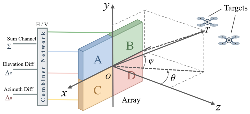
It is assumed that the radar operates under far-field and narrow-band conditions. Furthermore, within a sufficiently short observation interval, the variations in the target’s angular parameters and its polarization state are considered negligible. The system employs a dual-polarization three-channel monopulse antenna architecture, comprising the sum channel (
), the elevation difference channel (
), and the azimuth difference channel (
), as illustrated in
Figure 1. For the
m-th snapshot, the joint spatial-polarization sampled echo matrix
received from the radar mainlobe can be expressed as:
where
. The monopulse-ratio steering vector
and the polarization Jones vector
are defined as [
10,
21]:
where
and
denote the auxiliary polarization angle and the polarimetric phase difference, respectively.
and
represent the target’s monopulse ratios in elevation and azimuth, respectively.
Their relationships with the physical quantities in
Figure 1 are given by:
where
and
are the boresight directions of the radar mainlobe, and
and
are the actual elevation and azimuth angles of the target. For a uniform square array, the monopulse-ratio slopes are given by
, where
is the number of elements along each side of the array. This parameter directly determines the effective observation baseline of the array. Owing to the dimensionless nature of the monopulse ratio, the intrinsic performance of the proposed algorithm is decoupled from the specific radar antenna geometry and beamwidth. This characteristic ensures the universal applicability of the conclusions across diverse radar systems. In the subsequent sections, we focus on the estimation performance of the target monopulse ratios and provide a comprehensive analysis of the resulting 3D localization accuracy.
Based on (
1), the noisy mixed echo matrix for a dual-target scenario can be expanded as:
where
denotes the additive noise matrix. Its vectorized form,
, follows a zero-mean complex Gaussian distribution with a covariance matrix
, denoted as
. To ensure the identifiability of the dual-target angular resolution problem, we assume that the targets are spatially separated, i.e.,
. Furthermore, in practical observation scenarios, the targets typically exhibit distinct polarization states, represented as
. For clarity, the target-to-target power ratio
and the SNR are defined as:
4. Simulation Results
To comprehensively validate the validity of the aforementioned theoretical derivations, this section evaluates the performance of the proposed algorithm across various operational scenarios. To bridge the gap between abstract mathematical models and practical radar engineering, the subsequent evaluations are specifically designed to emulate challenging, real-world dual-target environments. The architecture and physical objectives of the simulation experiments are systematically mapped and summarized in
Table 1.
Each numerical result is derived from 300 independent Monte Carlo trials. Unless otherwise specified, the default azimuthal and elevational monopulse ratio (MR) differences between the two targets are set to 0.4 and 1.0, respectively. Target 2 is designated as the source located toward the upper-right region of the 2D angular plane. Under this configuration, as varies, the two targets traverse the mainlobe along parallel trajectories. Without loss of generality, the initial MR parameters are set to and , while the default polarization parameters are and .
To demonstrate the comparative superiority of the proposed method, we benchmark it against several state-of-the-art dual-target resolution algorithms that do not rely on polarimetric information. These include: the classical monopulse dual-target resolution method proposed by Blair [
10]; the maximum likelihood (ML)-based closed-form solution known as NM2 proposed by Wang [
13]; and the three-channel closed-form solution (Seung) [
14] tailored for slowly fluctuating targets. Furthermore, Blind Source Separation (BSS) [
19] and the latest polarimetric-enhanced method, Minimization of Polarimetric Variance (MPV) [
21], are also included for a comprehensive performance comparison.
4.1. Effectiveness of the Designed Cost Function
Given that the total search space encompasses four polarimetric parameters across the two targets, we fix the parameters of Target 1 at
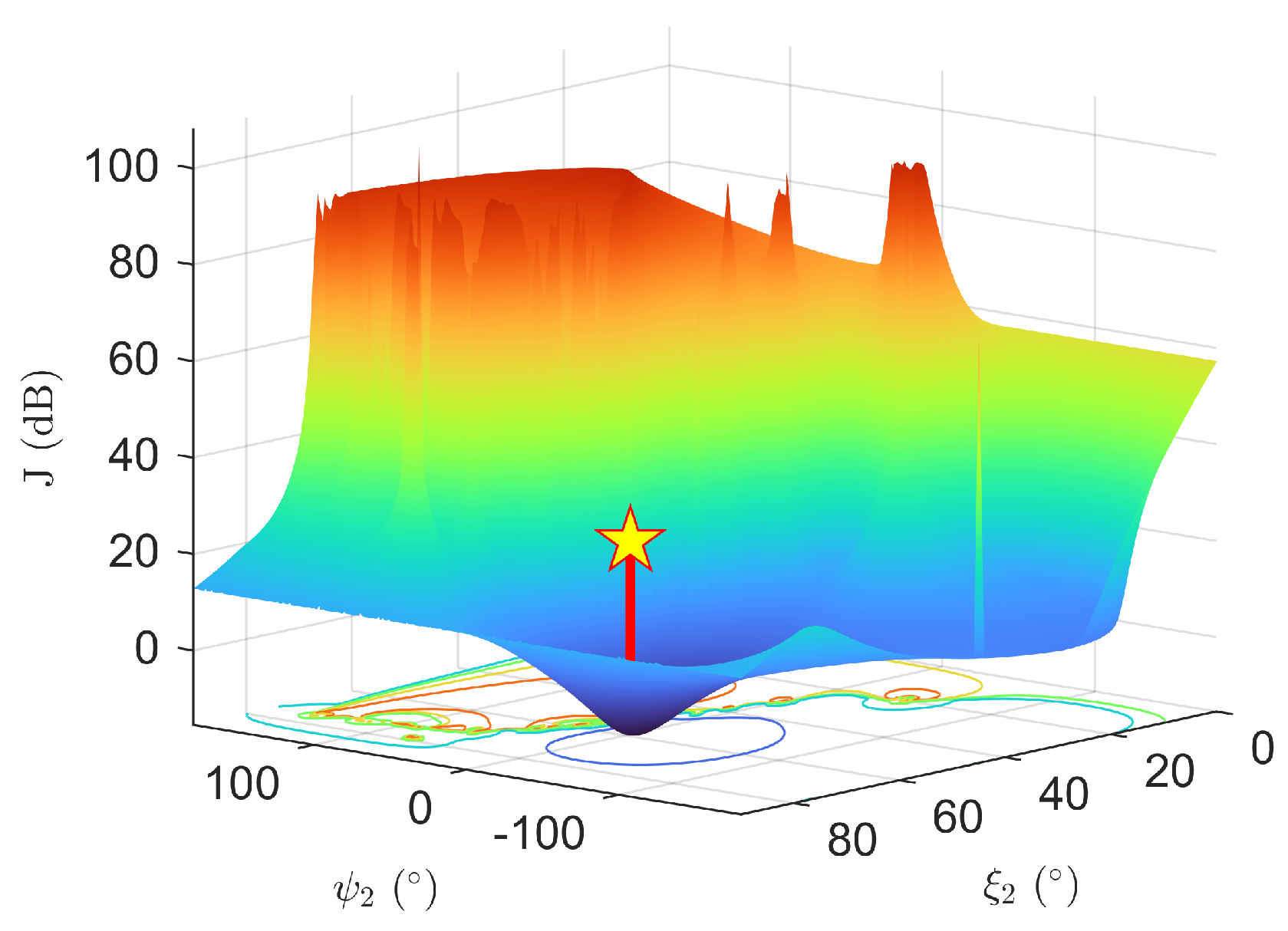
to facilitate a more intuitive visualization of the proposed cost function’s effectiveness. By performing an exhaustive parameter sweep of the remaining variables, the resulting optimization landscape is illustrated in
Figure 2. As observed, the cost function attains its global minimum precisely when the search variables align with the ground-truth polarimetric parameters of Target 2. This confirms that the designed cost function effectively guides the optimization process toward the true state of the second target, thereby validating its efficacy in directing the oblique projection for accurate signal component decoupling.
4.2. Solving Strategy and Algorithm Complexity
As can be observed, the optimization landscape reveals that the cost function is highly nonlinear and non-convex, characterized by irregular fluctuations rather than a smooth, monotonic profile. To handle such a complex search space and ensure robust convergence to the global optimum, we employ a Genetic Algorithm [
24] for parameter estimation in the subsequent numerical experiments. The specific hyperparameters, empirically tuned to balance global exploration and local exploitation, are summarized in
Table 2.
An elite fraction of is implemented, which guarantees that the top-performing individuals (the top ) from each generation are directly preserved and passed to the next generation without disruption. The crossover and mutation fractions specify that and of the next generation are produced by crossover and mutation operations, respectively.
For the crossover operation, a scattered crossover strategy (equivalent to uniform crossover) is employed. Given two parent individuals, the algorithm generates a random binary mask where each bit has an equal probability of being 0 or 1 to determine the origin of each dimensional gene for the offspring. This mechanism breaks the positional coupling between variables, thereby effectively enhancing the global exploration capability of the population within the solution space. Regarding the mutation operation, an adaptive feasible mutation strategy is employed. This mechanism generates offspring by introducing random perturbations to the parent individuals. It adaptively adjusts the mutation direction and step size based on the specific upper and lower bounds of the search variables, ensuring that all newly generated individuals strictly satisfy the feasible region constraints. Furthermore, the perturbation variance of this mutation operator dynamically decays as the number of generations increases. By maintaining a large step size in the early stages, it bolsters global exploration to avoid local optima; conversely, by shrinking the step size in the later stages, it significantly improves the convergence precision during local exploitation.
More importantly, for the specific 4D parameter optimization problem in this study, the cost function exhibits a pronounced approximate convexity in the immediate vicinity of the ground truth, as illustrated in
Figure 2. Benefiting from this favorable geometric property, the optimal solution obtained from each independent run of the genetic algorithm consistently converges to the true parameter basin, thereby ensuring the reliable reproducibility of the optimization results.
To rigorously validate that the optimization framework is robust and not overly sensitive to specific hyperparameter settings, we conducted a sensitivity analysis on two core GA parameters: Population Size and Crossover Fraction (note that with the elite fraction fixed at 0.05, the mutation fraction is deterministically assigned to satisfy the probability sum constraint). The estimation performance (Total MSE) under various configurations is summarized in
Table 3. As demonstrated, the angular estimation precision exhibits high stability across a wide range of hyperparameter configurations. Whether the population size spans from 50 to 600, or the crossover fraction varies from 0.6 to 0.8, the Total MSE for both targets consistently exhibits relatively minor fluctuations. The absence of drastic performance fluctuations confirms that the successful convergence of the proposed algorithm does not rely on carefully cherry-picked hyperparameters. Instead, it is fundamentally guaranteed by the inherent geometric properties of the cost function coupled with the robust population evolution strategy. Consequently, the chosen default configurations (e.g., Population = 400, Crossover = 0.8) are well-justified, providing a reliable balance between computational efficiency and global search capability.
To evaluate the computational efficiency of the proposed framework, we compared the actual execution times of the proposed GA-based method against the Seung method (solving quadratic equations) and the MPV method (algebraic cancellation). To ensure a fair comparison of the inherent algorithmic complexity, all methods were implemented using sequential (single-threaded) processing without any parallel computing acceleration. The simulations were performed on a computer equipped with a 12th Gen Intel(R) Core(TM) i9-12900H processor. The average computation times per single Monte Carlo trial over varying snapshots (
M) are summarized in
Table 4. As the results indicate, the MPV method is the most computationally efficient (operating in the millisecond range) due to its reliance on direct spatial cancellation operations. The Seung method requires moderate computation time that scales noticeably with
M.
Expectedly, the proposed method demands the highest execution time (averaging between 6 to 8 s) in a sequential software environment, which is the inherent cost of evaluating hundreds of individuals across multiple generations. However, two critical observations justify this computational overhead. First, the execution time of the proposed method does not scale exponentially with M; it remains relatively stable since the GA loop overhead dominates the minor matrix operations, corroborating our theoretical analysis. Second, and more importantly, evaluating individuals in a GA population is an “embarrassingly parallel” task. While the single-threaded execution takes seconds, implementing this algorithm on modern radar hardware platforms equipped with parallel processing units (e.g., FPGAs or GPUs) can drastically slash the computation time by orders of magnitude.
Ultimately, while the proposed framework requires increased computational resources in a sequential environment, it is a highly worthwhile trade-off. As will be comprehensively demonstrated in the subsequent experimental sections, conventional methods (like MPV and Seung) suffer from substantial performance degradation or even complete failure in challenging scenarios characterized by low SNR, severe power disparity, and fast-fading target environments. By contrast, the proposed method leverages this computational investment to guarantee superior robustness and high-fidelity 3D target imaging under these complex conditions.
4.3. Verification of Angular Estimation Performance
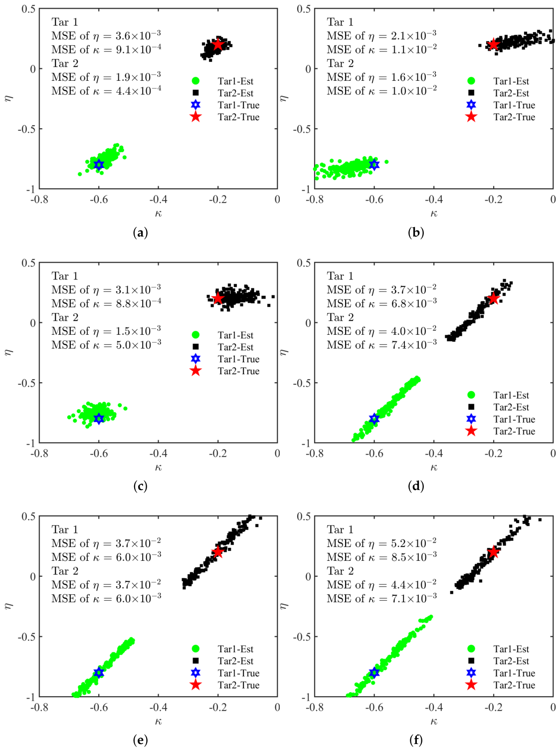
Under the conditions of SNR = 20 dB and a target power ratio of 0 dB with
snapshots, the angular estimation results are illustrated in
Figure 3. Note that the SNR and power ratio correspond to the signal components within the range cells after pulse compression.
Figure 3a displays the dual-target estimation results of the proposed method. The multiple measurements are accurately clustered around the ground truths with negligible bias and variance, successfully achieving high-precision resolution of mainlobe dual targets and laying a solid foundation for subsequent 3D imaging.
Figure 3b shows the results for the MPV method, which also utilizes polarimetric information. A distinct “horizontal stretching” trend is observed in the azimuthal scatter points, with the azimuthal monopulse ratio error increasing by an order of magnitude compared to the proposed method. The root cause is that MPV relies on polarimetric variance analysis after azimuth-domain cancellation. However, the cancellation process inevitably incurs power loss of the target signal, leading to reduced estimation precision. Since the azimuthal monopulse ratio difference in this experiment is significantly smaller than that in elevation, the performance degradation is more pronounced in the azimuth dimension.
Figure 3c presents the results of the three-channel closed-form solution (Seung). Since this method was specifically developed for slowly fluctuating dual-source scenarios, its overall performance is comparable to the proposed method.
In contrast, the classical dual-target resolution methods, Blair and NM2 (see
Figure 3d,e), exhibit “elongated” or “diagonal” scatter point distributions rather than compact clusters. This not only implies significantly increased uncertainty in angular estimation but also indicates a strong correlation error between the estimated
and
. Their performance degradation stems from the fact that these methods are designed for the Swerling II model, whereas the simulated echo envelopes are constant-modulus and Doppler-modulated. This model mismatch leads to a loss of algorithmic robustness. The worst performance is observed in the BSS method (
Figure 3f), characterized by the most diffuse scatter points. BSS relies on the accurate acquisition of a separation matrix, the estimation of which strictly depends on the statistical independence of the dual-source waveforms. At a low snapshot count (
) and with constant-modulus waveforms, the independence assumption is not sufficiently satisfied, rendering the algorithm unable to effectively lock onto the target positions and resulting in highly unstable measurements.
The experimental results confirm that at 20 dB SNR and with equal target power, the proposed method provides optimal estimation precision and robustness by effectively suppressing mutual interference between targets. Conversely, traditional methods exhibit significant performance degradation when facing model mismatch or limited snapshot scenarios.
Following the verification of the algorithm’s statistical robustness, this section further explores its practical application potential through a 3D localization scenario. By integrating high-precision angular estimation with range information, the targets’ 3D spatial coordinates can be accurately reconstructed.
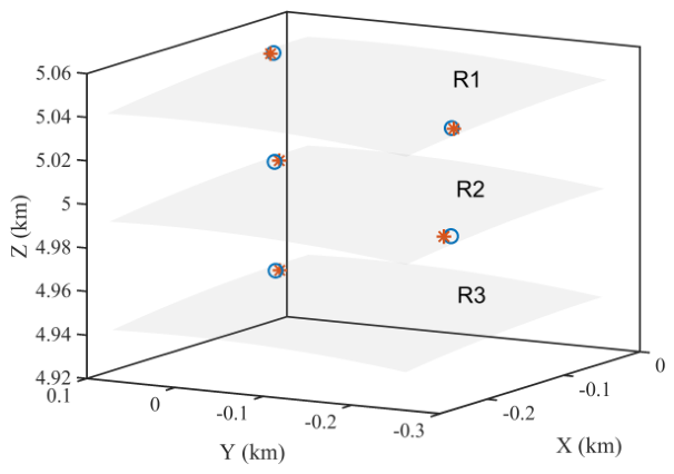
Figure 4 presents the 3D imaging results for multiple targets distributed across three distinct range bins (
km,
km,
km). Within each range bin, targets are assigned different velocities to ensure compliance with the non-coherence assumption.
In the figure, red stars represent the estimates derived from the proposed algorithm, while blue circles denote the ground-truth positions. The results clearly demonstrate a high spatial overlap between the estimated and true positions across all range bins, directly validating the critical role of high-precision angular estimation in accurate 3D imaging. Furthermore, the consistent performance across different range layers proves the algorithm’s robustness against range variations. Such superior spatial resolution capabilities fully confirm the effectiveness of the proposed approach for 3D imaging tasks involving point-target clusters in complex spatial configurations.
4.4. Sensitivity to Signal-to-Noise Ratio and Power Disparity
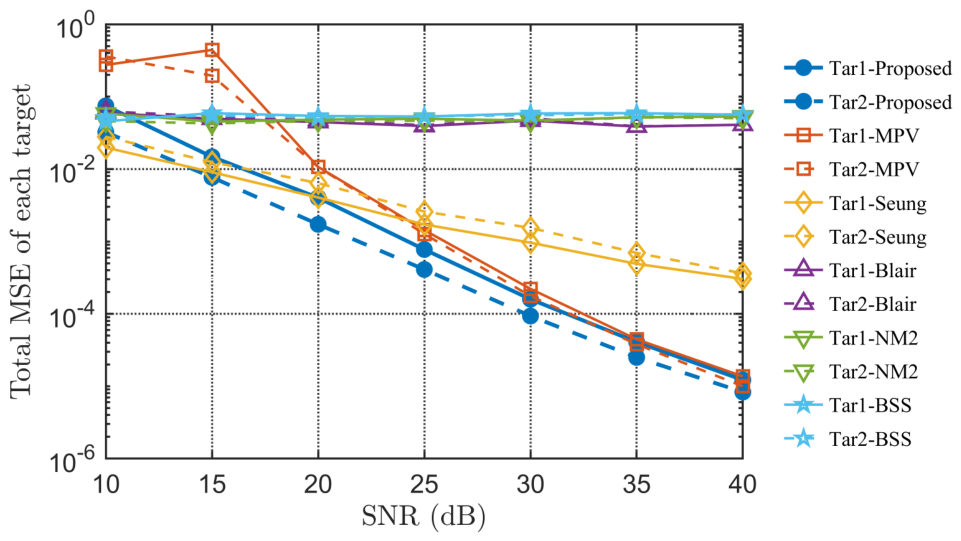
To further quantitatively evaluate the robustness and asymptotic performance of the proposed algorithm across varying noise environments, we conducted Monte Carlo simulations to analyze the relationship between the total MSE (defined as the sum of mean squared errors for both azimuth and elevation estimates) and the SNR, ranging from 10 dB to 40 dB. The comparative results are illustrated in
Figure 5.
As shown, the proposed method (indicated by the solid blue lines and dashed blue lines with circle markers) consistently achieves the lowest MSE across nearly the entire SNR range for both targets. Furthermore, the MSE exhibits a steady linear decline in the log-scale as the SNR increases. This demonstrates the algorithm’s superior capability in suppressing additive noise and its remarkable reliability under low-SNR conditions, where no sudden performance degradation (performance cliff) is observed.
In stark contrast, the classic Blair, NM2, and BSS methods exhibit a prominent “error floor” phenomenon. Their MSE curves remain nearly horizontal as the SNR improves beyond 15 dB. This saturation in performance reinforces our previous analysis regarding model mismatch: since these algorithms are fundamentally designed for Swerling II fluctuating models or rely on signal independence assumptions that are violated in this constant-modulus scenario, increasing the signal power cannot compensate for the inherent estimation bias caused by the mismatched signal manifold.
The MPV method shows a significant performance gap at low SNR levels (10–20 dB), which can be attributed to its increased sensitivity to noise resulting from the power loss incurred during the target cancellation process. However, as the SNR exceeds 25 dB, its performance gradually converges with the proposed method, indicating that the impact of power loss becomes less dominant when the noise floor is sufficiently low. Meanwhile, although the Seung method is more robust than the Blair/NM2 group, it exhibits a shallower slope compared to the proposed method. This suggests that the Seung method achieves lower performance gains from increasing SNR than our approach. Overall, the curves in
Figure 5 validate that the proposed algorithm not only maintains high precision under high-SNR conditions but also provides exceptional reliability in challenging noise environments.
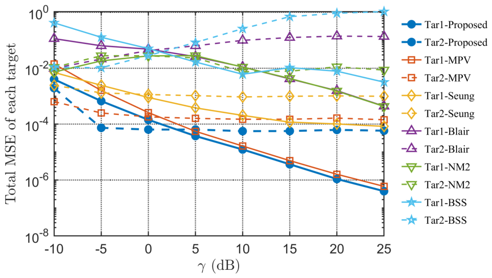
Beyond the SNR, the power ratio between spatially adjacent targets is a crucial metric for assessing algorithmic robustness. In practical radar detection, significant power imbalances frequently arise due to differences in the targets’ RCS or radial distances. To this end, this section investigates the variations in angular MSE as a function of the power ratio (ranging from −10 dB to 25 dB), with the SNR of Target 2 fixed at 30 dB. As illustrated in
Figure 6, the proposed method (solid and dashed blue lines) consistently achieves the minimum estimation error across the entire range of
. Even under conditions of extreme power imbalance (e.g.,
dB), the estimation precision for both strong and weak targets remains stable at a low level, significantly outperforming the competing methods. This demonstrates that the proposed algorithm effectively decouples the overlapped signals and successfully suppresses the “capture effect” of dominant targets on weaker ones, exhibiting superior stability across a wide dynamic range.
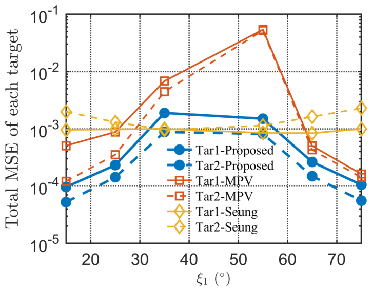
In contrast, the classical Blair, NM2, and BSS methods suffer from drastic performance degradation as the power ratio deviates from the balanced state (0 dB). Specifically, when Target 1 is substantially stronger than Target 2, these algorithms fail to accurately lock onto the signal components of the weaker target, leading to a complete failure in angular estimation. This observation further validates our prior theoretical analysis: since these baseline methods depend heavily on specific statistical properties of signal envelopes, they lack the robustness to resolve components when the energy levels are vastly different. While the MPV and Seung methods are more stable than the Blair group, their MSE curves exhibit a relatively high “performance floor.” Although the MPV method shows improved precision for the stronger target as increases, its error for the weaker target remains much higher than that of the proposed approach, highlighting the limitations of cancellation-based methods under asymmetric power conditions.
In summary, the MSE curves across varying power ratios verify that the proposed method not only excels at low SNR but also effectively handles significant power disparities. Such high-precision angular estimation capability within a wide dynamic range is of great practical value for 3D imaging and reliable tracking in complex environments, such as scenarios involving targets with diverse RCS or strong background clutter.
4.5. Impact of Spatial Angular Separation
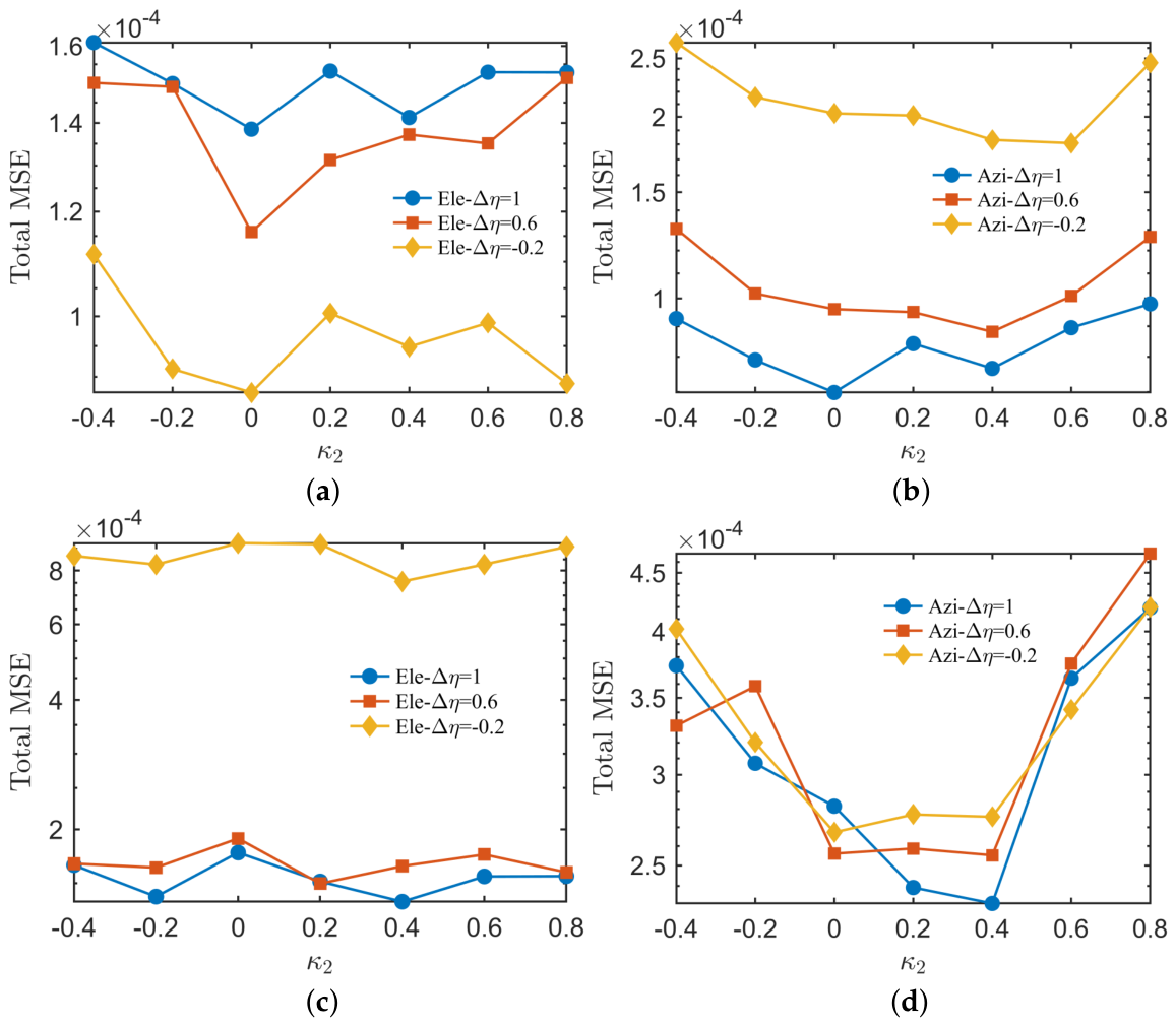
Next, we explore the impact of angular separation on estimation accuracy. In practical scenarios, the most stringent challenge in mainlobe multi-target resolution arises when targets are extremely close spatially, leading to severe overlap in the signal manifold. To this end, we vary the elevation difference
(setting it to 1, 0.6, and 0.2) while traversing the azimuth coordinate
, to comparatively analyze the MSE of the proposed method and the relatively better-performing MPV method in both elevation (Ele) and azimuth (Azi) dimensions. It should be emphasized that the “Total MSE” here refers to the sum of MSEs for the two targets within a specific angular dimension, rather than the sum across both dimensions for a single target. As illustrated in
Figure 7a,b, the proposed method exhibits exceptional stability across different spatial separations. Notably, as the elevation separation
decreases from 1 to 0.2 (where a separation of 0.2 corresponds to approximately 0.1 of the mainbeam width), the estimation errors in the azimuth and elevation dimensions manifest divergent trends. As
increases, the azimuthal monopulse ratio precision improves, whereas the elevation precision declines. This phenomenon occurs because the estimation accuracy is simultaneously governed by the similarity of the spatial steering vectors and the specific parameter values. While increasing the angular difference in one dimension enhances the decoupling capability for the other dimension, it simultaneously expands the potential fluctuation range of the estimates within its own dimension, leading to a slight increase in variance. Nevertheless, the total MSE remains consistently below
, demonstrating the algorithm’s ability to effectively leverage joint spatial-polarimetric features and achieve high spatial resolution through precise oblique projection decoupling.
By comparing
Figure 7c,d, it can be observed that for the MPV method, the elevation precision improves as
increases, while the azimuth precision remains nearly unchanged. This creates a distinct contrast with the trends observed in the proposed method. The reason lies in the core principle of MPV, which performs angular estimation sequentially by nulling one target before estimating the other’s coordinates. Consequently, a smaller angular separation leads to more severe signal self-cancellation (power reduction) during the nulling process, causing a collapse in the effective SNR and significant performance degradation in small-separation scenarios. Furthermore, performing the cancellation within each respective dimension effectively decouples them, thereby mitigating inter-dimensional interference. In contrast, the proposed method first estimates the 3D spatial steering vector (comprising
,
and
) and then extracts the angular parameters, which inherently introduces mutual influence between dimensions. However, the results confirm that this joint utilization of 2D angular information leads to higher overall robustness and superior estimation precision, further validating the advantages of the proposed framework.
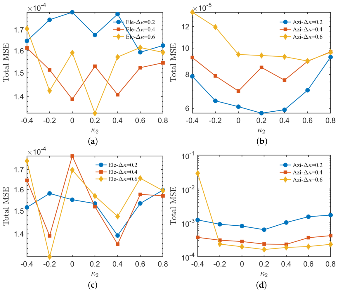
To further verify the universality of the aforementioned physical mechanism, we investigate the impact of azimuthal spatial separation (
) on angular accuracy. By fixing the elevation difference and varying the azimuthal separation
(set to 0.2, 0.4, and 0.6), we conduct a comparative analysis of the MSE trends for both the proposed and MPV methods, as illustrated in
Figure 8.
As observed in
Figure 8a,b, the proposed method exhibits a highly symmetrical “cross-dimensional gain” phenomenon relative to the
experiments. As the azimuthal separation
increases, the elevation (Ele) precision (
Figure 8a) shows a significant improvement. Conversely, the azimuth (Azi) precision itself (
Figure 8b) slightly decreases as
grows. This result once again validates the joint estimation characteristic of the proposed method: when the angular divergence in one dimension increases, the overall discriminability of the spatial steering vector is enhanced, thereby providing more robust geometric features for decoupling the other dimension. The slight decline in azimuth precision is, as previously discussed, due to the expansion of the physical search space for parameter estimation as the angular difference increases, leading to a marginal rise in statistical variance. Nonetheless, at an SNR of 30 dB and under the extremely stringent condition of
, the proposed method maintains an ultra-high precision of the
order, demonstrating its robust performance near the resolution limit.
In contrast, the MPV method exhibits significant performance imbalance and extreme sensitivity to spatial separation. As shown in
Figure 8d, at
, the azimuthal MSE of MPV surges to the
level, which is attributed to severe power loss and the collapse of effective SNR during the azimuthal cancellation process in small-separation scenarios. Meanwhile, its elevation precision (
Figure 8c) remains relatively less affected by
variations due to the dimensional decoupling inherent in its architecture.
In summary, the comprehensive comparison reveals that the proposed method, by jointly utilizing three-channel spatial information, effectively avoids the “signal self-cancellation” trap typical of cancellation-based methods like MPV. Whether in scenarios with varying or , the proposed method leverages inter-dimensional correlation to achieve performance complementarity, ensuring stable and high-precision 3D localization results under complex spatial configurations.
4.6. Impact of Sample Size
In
Figure 9, we further investigate the impact of the number of snapshots (
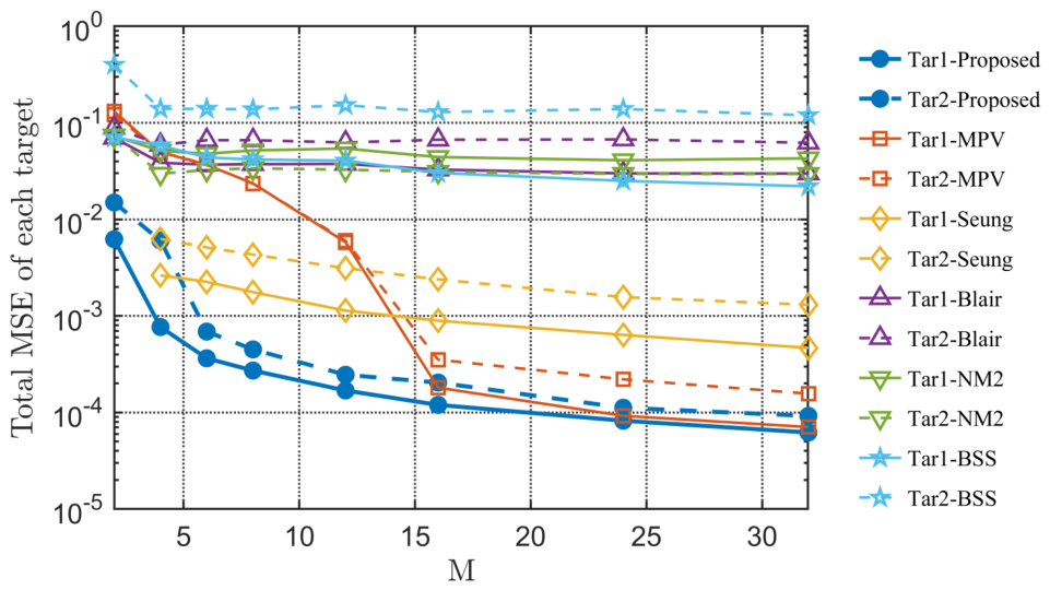
M) on angular estimation performance. In practical dynamic imaging scenarios, targets typically exhibit rapid angular dynamics (i.e., fast variations in the target’s angular coordinates relative to the radar boresight). This necessitates high-precision localization within extremely short dwell times to satisfy the assumption of parameter stationarity, thereby limiting the available number of snapshots. To this end, we varied
M from 2 to 32 and compared the total MSE among the compared methods, as illustrated in
Figure 9.
The proposed method (blue curve) demonstrates exceptional sample efficiency. Even under the stringent condition of an extremely low number of snapshots, its estimation error rapidly converges to below the order, maintaining a steady and continuous decline as M increases. This result confirms that the proposed method effectively exploits the joint polarimetric-spatial features from limited data, making it highly suitable for rapid target imaging tasks with demanding real-time requirements.
In contrast, the MPV method (orange curve) exhibits significant performance fluctuations in low-snapshot scenarios. Specifically, when , its MSE remains relatively high with a slow convergence rate, indicating that the MPV method’s dependence on data volume is notably higher than that of our algorithm. Notably, traditional methods such as Blair, NM2, and BSS once again manifest pronounced performance bottlenecks. Even as M increases to 32, their MSE curves persist at a high “error floor” with negligible improvement. This further corroborates our earlier conclusion: due to the inherent model mismatch between these methods and the “constant-modulus phase-modulated” signal model used in our experiments, increasing the sample size (snapshots) can only mitigate the impact of random noise but cannot eliminate the structural bias caused by the mismatched model.
In summary, the results indicate that for a given precision requirement, the proposed method requires the fewest snapshots, offering optimal convergence speed and real-time processing potential. In complex dynamic remote sensing applications, this high-efficiency processing capability for low-snapshot data is key to ensuring high-frame-rate and high-precision 3D imaging.
4.7. Impact of Waveform Characteristics
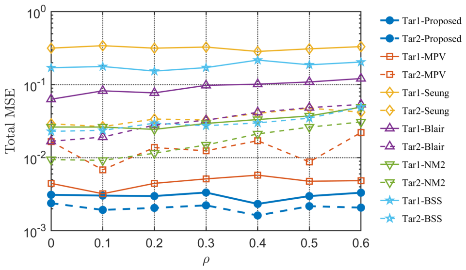
The core principle of the proposed cost function lies in exploiting the non-coherence between source waveforms—specifically, by achieving signal decoupling through the induced fluctuations in the monopulse angular measurement of the synthesized signal, which are driven by the asynchronous fluctuations of the complex echo envelopes. To evaluate the algorithm’s robustness in complex environments, such as partially coherent scenarios, the angular estimation performance among the compared methods is first investigated under two typical mechanisms for controlled waveform correlation. The first configuration (
Figure 10) isolates the effect of amplitude fluctuations on the correlation coefficient
, representing two targets moving at identical radial velocities but possessing distinct radar cross-section (RCS) amplitude scintillation. The second configuration (
Table 5) relies solely on inter-snapshot relative phase variations to adjust the correlation, corresponding to targets with stable RCS but exhibiting Doppler frequency disparities due to relative motion. This orthogonal experimental design facilitates a detailed analysis of the algorithm’s performance boundaries under different decorrelation mechanisms.
As observed in
Figure 10, the proposed method (blue curve) exhibits exceptional robustness across the entire range of
. Even when the correlation between the two source signals increases to 0.6, the angular MSE remains tightly locked within the
order, with the curve remaining nearly flat and showing no significant performance degradation. In contrast, the MPV method (orange curve) exhibits a slight upward trend in MSE as the correlation
grows, with its estimation error remaining consistently higher than that of the proposed method. Methods such as BSS (Blind Source Separation) and Blair/NM2 are even more drastically affected by waveform correlation. This is primarily because BSS-like methods rely heavily on the assumption of statistical independence. When the waveform correlation increases, the underlying assumptions of their mathematical models are violated, leading to deteriorated estimation results. These findings demonstrate that the proposed method possesses superior robustness against partial correlation induced by stochastic envelope amplitude fluctuations, effectively ensuring 3D imaging fidelity even when waveform independence is compromised.
As illustrated in
Table 5, the angular estimation MSE for nearly all algorithms manifests a significant upward trend as the correlation coefficient
increases. Notably, compared to the stochastic amplitude fluctuation scenario (
Figure 10), this constant-modulus case characterized by gradually evolving phases generally leads to higher estimation errors. For the proposed method, although the statistical correlation across snapshots is consistent with the amplitude-fluctuating scenario, the phase difference between the two source waveforms evolves linearly over time. This deterministic evolution pattern constrains the instantaneous volatility of the composite signal within each snapshot, thereby limiting the efficacy of signal decoupling based on the fluctuation-minimization criterion. The MPV method, which also exploits waveform non-coherence, similarly exhibits a performance degradation compared to the results in
Figure 10. The NM2 method exhibits a similar performance profile under both mechanisms of partial correlation, as its estimation error is primarily driven by model mismatch and remains largely insensitive to the specific physical origins of waveform correlation. Nevertheless, its MSE is consistently higher than that of the proposed method; this is because whether the correlation arises from amplitude fluctuations or phase variations, the underlying assumption of independent Rayleigh-distributed target amplitude fluctuations is fundamentally invalidated. Furthermore, while the Seung method is specifically tailored for constant-modulus sources, its robustness necessitates sufficient phase diversity between snapshots; the gradual nature of the phase evolution in this scenario provides insufficient variation, thereby adversely affecting its angular resolution accuracy.
In summary, the controlled waveform correlation experiments demonstrate that the proposed method consistently outperforms existing techniques under partially correlated conditions. However, to maintain high estimation accuracy when the partial correlation stems solely from deterministic phase variations (e.g., constant-modulus signals with Doppler-induced phase evolution), the correlation coefficient must remain relatively low. For example, using a 256-element square array with an approximate beamwidth of 6.35°, the proposed algorithm maintains a monopulse ratio MSE below 0.01 provided that the Doppler-induced correlation does not exceed 0.1. This translates to an angular root-mean-square error (RMSE) of roughly 0.45° [
25]—achieving an exceptional precision that is less than one-tenth of the beamwidth.
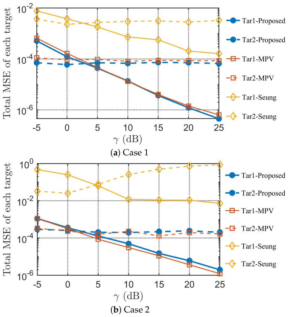
While the aforementioned orthogonal experiments have analyzed algorithmic performance under specific controlled correlation mechanisms, we now return to the primary focus of this study: scenarios where the two source waveforms are nearly completely non-coherent. To evaluate the robustness of the three top-performing methods identified thus far (Proposed, MPV, and Seung) across varying inter-source power ratios (
), we extend our analysis to more generalized non-coherent waveform models. Specifically, Case 1 features constant-modulus (CM) echoes with stochastic random phases, representing the coexistence of non-coherent co-channel interference and a target. Case 2 employs the Swerling II model, characterized by independent, stochastic complex envelope fluctuations, simulating two typical fast-fading targets. The comparative results are illustrated in
Figure 11.
By comparing Case 1 and Case 2 in
Figure 11, it is evident that the statistical properties of the signal envelope significantly impact angular accuracy. In Case 1 (CM), the stable signal power across snapshots provides a consistent effective SNR gain, resulting in low MSE for all methods. In contrast, for Case 2, the random fluctuations of the RCS lead to low instantaneous SNR in certain snapshots, causing a general rise in estimation errors across all algorithms. This observation aligns with the physical principles regarding the constraints imposed by stochastic fading on estimation precision in radar signal processing.
Under the current simulation parameters, the proposed method (blue curve) and the MPV method (orange curve) exhibit a high degree of consistency, with their curves nearly overlapping in both signal models. This indicates that at a relatively high SNR (30 dB) and with sufficient angular separation, both the polarimetric oblique projection optimization strategy (Proposed) and MPV possess excellent robustness against target power imbalance. However, the Seung method (yellow curve) suffers from severe performance degradation in the fluctuating environment of Case 2. This degradation aligns consistently with the results from the controlled correlation experiments, where the Seung method exhibited heightened vulnerability to inter-snapshot amplitude fluctuations. It further confirms that this approach struggles to accurately lock onto weak target positions in fast-fading environments.
In conclusion, comprehensive comparisons across diverse waveform characteristics reveal a fundamental insight: whether the sources are fully non-coherent or partially coherent, the specific physical mechanism driving the waveform correlation (e.g., amplitude scintillation versus phase progression) inherently dictates the resulting angular estimation performance. Consequently, algorithmic efficacy varies significantly depending on the underlying echo model. Nevertheless, amidst these waveform-induced variations, the proposed method consistently demonstrates the utmost robustness and the highest angular estimation precision among all evaluated techniques. This exceptional reliability establishes a solid foundation for subsequent high-fidelity 3D target imaging.
4.8. Impact of Polarimetric Diversity
Polarization diversity serves as a critical physical dimension for resolving non-coherent sources within the radar mainlobe. Consequently, we examine the limitations imposed by polarimetric feature disparity on multi-target resolution. Specifically, both sources are configured as purely linearly polarized targets by setting their polarimetric phase differences to zero (
). Subsequently, by fixing the auxiliary polarization angle of Target 2 at
and continuously varying
of Target 1, we obtain the curves of angular MSE as a function of the polarimetric disparity, as illustrated in
Figure 12.
As observed, when approaches , the MSE of both algorithms that exploit polarization diversity (Proposed and MPV) increases significantly. This performance saturation occurs because, as the targets’ polarization states become more similar, the polarimetric manifold of the mixed echoes undergoes degeneracy. This leads to enhanced ill-conditioning of the oblique projection matrix in the proposed method and the failure of the MPV method’s evaluation function. In contrast, the Seung method, which does not utilize polarization diversity, maintains relatively stable overall performance. However, in regions with substantial polarimetric disparity, its MSE is approximately one order of magnitude higher than that of the polarimetric-enhanced methods.
To theoretically comprehend the performance bounds under polarimetric degeneracy, it is crucial to analyze the conditioning of the OP matrix. In the 2D polarization space, the Jones vectors are normalized. The core inversion operation in the OP matrix
reduces to a scalar computation:
. For the linearly polarized targets simulated here (
), this scalar simplifies elegantly to
, where
represents the polarimetric angular disparity [
26].
This derivation reveals a fundamental theoretical boundary: the noise amplification factor during signal decoupling is directly proportional to
. As the polarimetric states converge (
), the OP matrix becomes increasingly ill-conditioned, and the projected noise power approaches infinity. Therefore, the minimum required polarization difference is not an absolute constant, but rather a dynamic threshold dependent on the ambient Signal-to-Noise Ratio (SNR). As visually confirmed in
Figure 12, under the current configuration of SNR = 30 dB, the algorithm maintains robust spatial resolution as long as
is greater than 10°. Once the disparity falls below this boundary, the drastically amplified noise overwhelms the target components, leading to a surge in estimation MSE.
Overall, the proposed method achieves the most favorable results. Compared to the MPV method, where the estimation error surges rapidly as the polarization states converge, the proposed approach demonstrates superior robustness against polarimetric similarity. These findings further validate the efficacy and rationality of utilizing both polarimetric oblique projection and angular fluctuation stability as the core components of our designed cost function.
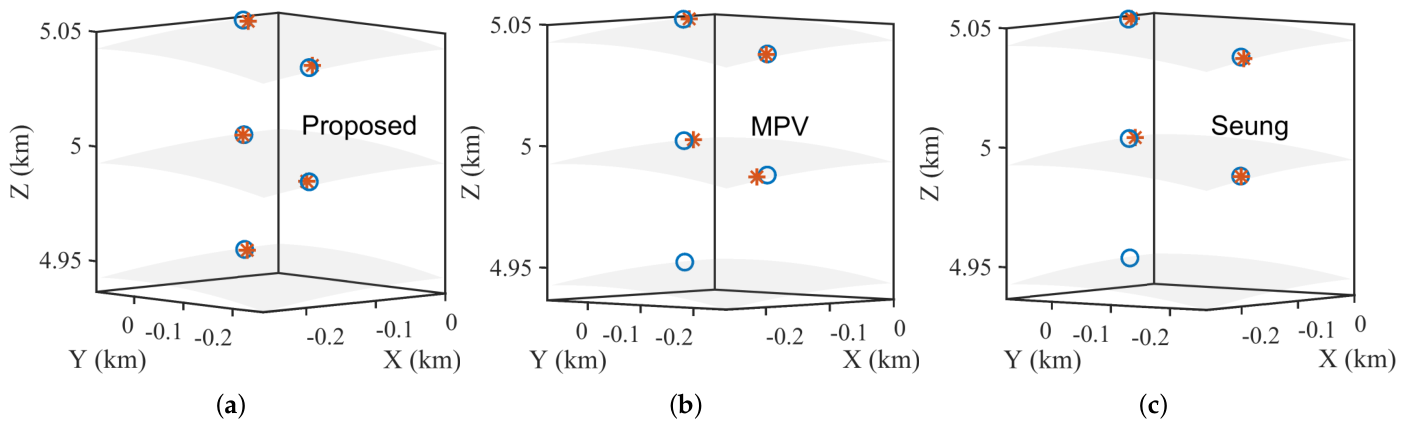
To intuitively evaluate the reconstruction fidelity in polarimetrically challenging scenarios,
Figure 13 presents the 3D imaging results when the auxiliary polarization angle difference is restricted to only 10°. For the proposed method, the estimated coordinates (blue circles) and ground-truth positions (red stars) exhibit nearly perfect overlap. This demonstrates that the algorithm can achieve high-fidelity 3D coordinate extraction even when the target discriminability in the polarimetric domain is relatively weak. In contrast, the MPV method suffers from significant positioning biases, with several estimated points deviating markedly from the ground truth. Meanwhile, the Seung method, although capturing the general spatial trend, exhibits visible estimation errors in specific range bins.
The experimental results suggest that the proposed framework possesses higher sensitivity to and more efficient utilization of polarimetric feature disparities. Even under the condition of weak polarimetric diversity, the algorithm maintains superior accuracy in 3D point-cloud reconstruction. More importantly, the baseline methods (MPV and Seung) fail to resolve targets correctly when only a single source is present, highlighting their reliance on prior target enumeration, which limits their practical utility. Conversely, the proposed method is fundamentally based on waveform separation. Whether the scene contains one or two sources, the optimized oblique projection ensures that the separated signal components consistently retain the correct spatial angular information. This set of simulations provides robust evidence for the application of the proposed method in robust anti-interference remote sensing and high-density civilian traffic monitoring.
5. Experimental Validation with Field-Measured Data
With the dense deployment of wireless infrastructure in coastal areas, radars tasked with maritime traffic management frequently encounter active radio frequency (RF) interference from nearby co-channel communication base stations or non-cooperative civilian radars. To validate the effectiveness of the proposed algorithm in complex co-channel overlapping scenarios involving non-coherent sources, we conducted an experimental verification using field-measured data.
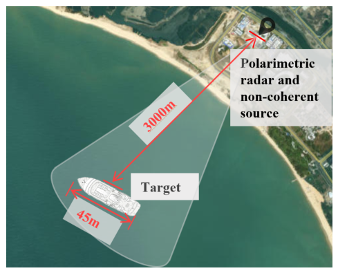
Figure 14 illustrates the experimental configuration. The campaign was carried out in a coastal environment, where a shore-based three-channel polarimetric radar was deployed on a high vantage point, alongside a stationary RF source simulating such non-cooperative co-channel emissions. The target under observation is a civilian vessel with a length of 45 m, situated approximately 3000 m from the radar. The detailed system parameters and specific configurations for the target and the interference are summarized in
Table 6.
Although the civilian vessel is a spatially distributed target, our method focuses on the high-precision estimation of its Equivalent Phase Center (EPC). In practical civilian applications—such as maritime traffic management, route guidance, or autonomous collision avoidance for radar-equipped vessels—acquiring the precise angular centroid of an obstacle is crucial and practically sufficient.
To correctly interpret the subsequent estimation accuracy, the acquisition method of the angular ground truth (represented by the red and blue stars in the subsequent figures) and the physical nature of this EPC must be clarified. The ground truth was not acquired via optical or GPS means; instead, it was independently established using the radar’s own high-precision monopulse measurements in a “clean” electromagnetic environment. Specifically, for the civilian vessel target, the reference coordinates were recorded just prior to the activation of the active co-channel interferer. Conversely, for the active interferer itself, the ground truth was determined by operating the radar in a passive reception mode (without transmitting) to locate the emission source, and the temporal mean of these measurements was adopted as the absolute reference.
Regarding the reference point on the ship, the reported ground truth does not correspond to the ship’s geometric centroid. During the experimental campaign, a trihedral corner reflector (with an edge length of 70 cm) was strategically deployed on the vessel. Given the radar’s 100 MHz bandwidth (providing a range resolution of roughly 1.5 m), the spatially extended ship is resolved across multiple range cells. By extracting the peak after pulse compression, the received data within the target cell is overwhelmingly dominated by the corner reflector, which effectively anchors the EPC and significantly suppresses severe structural angular glint.
However, due to residual scattering from the ship’s local structure and the potential influence of sea-surface multipath, the extracted reference angle is not the absolute geometric coordinate of the corner reflector alone. Rather, it represents a composite EPC formed by the dominant corner reflector superimposed with these environmental effects. To mitigate the detrimental impact of diffuse (non-coherent) multipath, we smoothed out the induced rapid angular fluctuations by extracting only a single stable angular snapshot per coherent processing interval (CPI). Furthermore, for specular multipath, because the physical deployment height of the reflector is relatively low, the angular divergence between the direct path and the multipath reflections is extremely small. From the radar’s macroscopic perspective, these components are highly clustered and can be reliably treated as composite echoes originating from the same spatial angle.
Therefore, we reiterate that while a microscopic electromagnetic analysis of structural glint and multipath fading is critical in target scattering modeling, it falls beyond the scope of this study. Our primary focus remains strictly on isolating this stable composite target EPC from severe non-coherent co-channel interference to provide robust coordinate support.
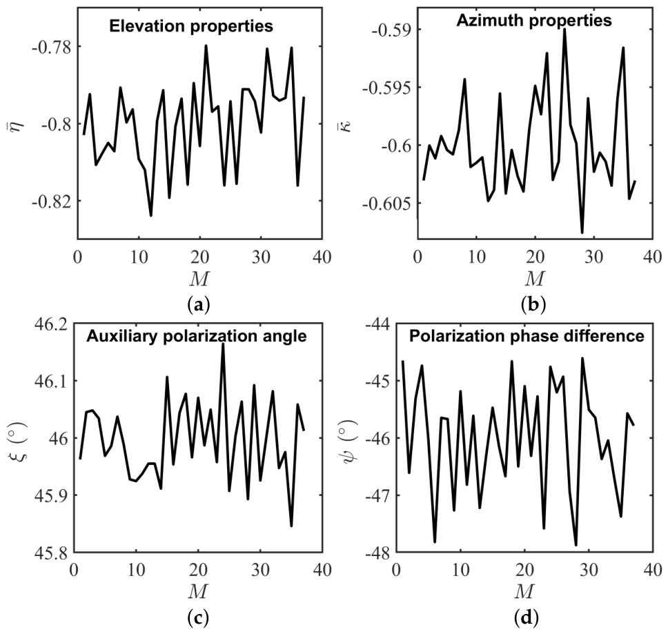
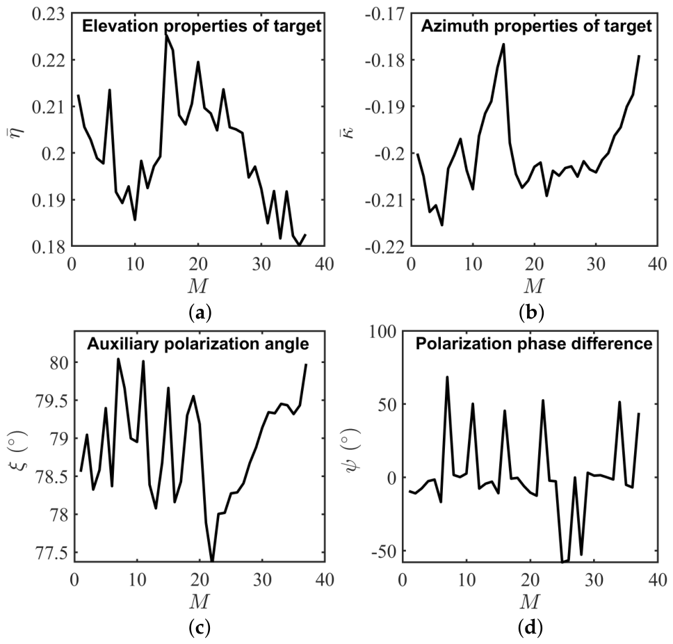
To empirically demonstrate the dynamic characteristics of the aforementioned ground-truth measurements,
Figure 15 and
Figure 16 illustrate the snapshot-to-snapshot variations of the isolated civilian vessel and the active interferer, respectively.
For the isolated ship echoes, the azimuthal and elevational monopulse ratios (
and
) in
Figure 15a,b reveal the inherent spatial instability of the target. Despite a relatively steady navigation state, subtle attitude variations (e.g., pitch and roll) induced by sea waves cause abrupt interference phase changes among residual scattering centers. This triggers a noticeable angular glint phenomenon, leading to rapid snapshot-to-snapshot drift of the EPC. However, as clearly observed from the results, the magnitude of these irregular angular fluctuations remains strictly bounded within a narrow margin. This bounded variance empirically justifies our previous assertion: from a macroscopic radar perspective, the composite echo can still be validly approximated as originating from a single point-like target.
In the polarimetric domain,
Figure 15c,d highlight a unique “Stable-Amplitude Random-Phase Scintillation” effect. The auxiliary polarization angle (
) fluctuates within a tight range of 77° to 80°, indicating that the power ratio between the vertical and horizontal polarization channels remains consistent during the observation. In stark contrast, the polarimetric phase difference (
) exhibits large-scale, pseudo-random jumps between −50° and 70°. This confirms that real-world extended targets possess highly complex, fast-fading polarimetric signatures that far exceed the complexity of idealized simulated models.
Conversely, the measurements of the active interferer operating in passive reception mode (
Figure 16) exhibit high parametric stationarity across both spatial angles and polarimetric states. Theoretically, the proposed oblique projection framework relies on the assumption that the polarimetric states of the sources remain stable over the short observation window. The intense polarimetric phase scintillation of the ship seemingly violates this strict assumption, making it physically challenging to define a single, absolutely accurate oblique projection operator for the target.
However, this highlights the inherent robustness of the proposed fluctuation-minimization criterion. Instead of relying on a fixed polarimetric prior, the optimization process is driven entirely by minimizing the spatial angular jitter of the decoupled components. Consequently, even in the presence of target polarimetric fluctuations, the algorithm adaptively converges to an “optimal equivalent” polarization state to enforce the most mathematically correct waveform separation possible. As will be explicitly demonstrated by the subsequent target-interference resolution results, this mechanism successfully minimizes the residual angular variance and achieves highly robust signal decoupling in non-ideal, real-world environments.
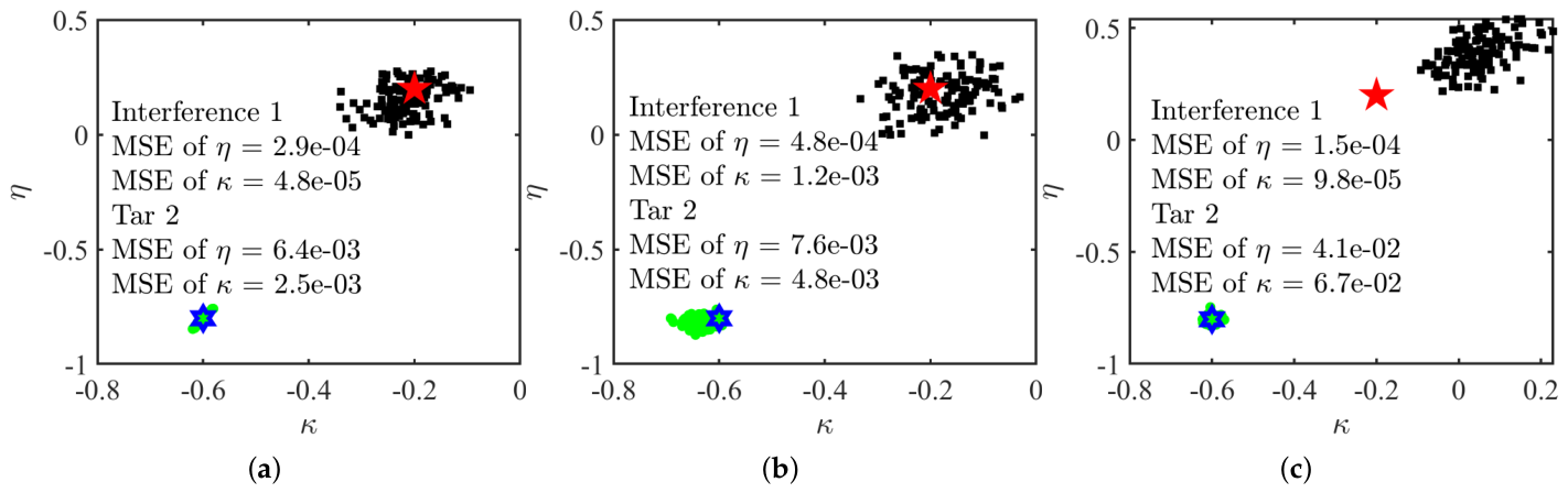
Based on the experimental configuration described previously, we further verify the resolution performance of the compared algorithms in a real-world complex electromagnetic environment. Statistical processing was conducted on 100 data segments. Each segment comprises sampling snapshots, where each snapshot corresponds to the sample extracted precisely at the peak position in the range-Doppler domain. By comparing the estimation results of the three top-performing algorithms—Proposed, MPV, and Seung—against the non-coherent interference and the civilian vessel target, we evaluate their practical effectiveness in engineering applications.
Figure 17a displays the processing results of the proposed method. It is evident that the estimated coordinates for the interferer (green dots) and the target (black dots) are tightly and accurately clustered around their respective ground truths (red and blue stars). This result provides robust evidence of the proposed algorithm’s superiority in real-world scenarios.
Figure 17b presents the results for the MPV method. Although MPV can roughly distinguish the target from the interference, its scatter points are significantly more diffuse than those of the proposed method. The underlying reason is that the precision of MPV relies on the stability of polarimetric parameters after target cancellation. However, as per our earlier analysis of the ship’s physical echo characteristics, the intrinsic polarimetric fluctuations of the source itself negatively impact the convergence of the parameter estimation process. Even if the cancellation is successful, these fluctuations persist. In contrast, the proposed method utilizes the angular-domain stability as the guiding metric for convergence and employs a joint 2D (azimuth-elevation) estimation strategy, leading to significantly higher robustness.
The worst performance is observed in the Seung method (
Figure 17c), where the estimated scatter points for the target (black) exhibit a pronounced bias relative to the ground truth (red star). This pronounced bias reveals the inherent limitations of the three-channel closed-form solution. Lacking the additional degrees of freedom provided by polarimetric diversity, its idealized statistical assumptions suffer from severe model mismatch when confronted with the highly dynamic envelope and phase scintillations of real-world extended targets. Consequently, it is entirely overwhelmed by the strong active emission, rendering it incapable of effective signal decoupling under such high ISR conditions.
In summary, the results from field-measured data processing directly demonstrate the superior performance of the proposed algorithm in resolving non-coherent sources in real-world scenarios. With a limited count of only 16 snapshots, the proposed method yields the most compact and accurate angular measurements, providing reliable technical support for high-resolution imaging in complex mainlobe jamming environments.
To intuitively demonstrate the spatial resolution and reconstruction capabilities of the proposed algorithm in practical complex scenarios, this section fuses the angular estimation results with radar range information to reconstruct the 3D point cloud of the observed scene.
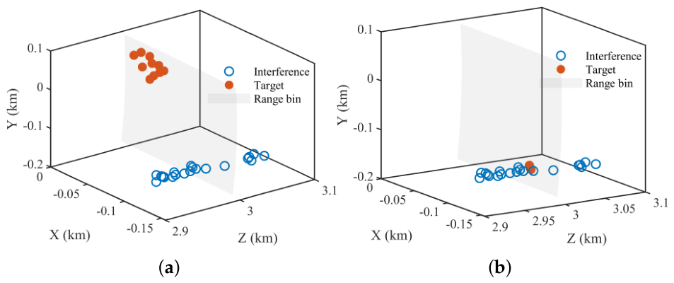
Figure 18 compares the 3D point-cloud reconstruction capabilities of the proposed framework against the conventional Direct Monopulse Ratio (DMR) method in a realistic co-channel interference scenario. Given that the proposed framework is universally applicable to both single-target and multi-target scenarios, we present the 3D imaging results of the sources near the target’s range gate. In the figure, the red solid dots represent the reconstruction results of 10 independent observations of the target within the current range cell, while the blue open circles represent the interference signals distributed across different range cells. The shaded region clearly delineates the physical range gate of the target.
As illustrated in
Figure 18a, the proposed method successfully achieves a precise spatial stripping of the target from the interference in 3D space. Although both the target (red) and the interferer (blue) are spatially overlapped within the radar mainlobe, the algorithm accurately extracts the target’s true angular parameters through the oblique projection decoupling operator. The reconstructed target points exhibit a high degree of focus (clustering) and are precisely located within the target’s designated range gate. Simultaneously, the interference signals are correctly reconstructed across their respective range cells, forming a clear and discriminable boundary in 3D space. This performance validates the algorithm’s capability to extract high-fidelity 3D geometric centroids even under intense interference-to-signal ratio (ISR) conditions.
In contrast,
Figure 18b reveals that the conventional DMR method entirely fails in this scenario. Due to the presence of strong non-coherent interference (ISR = 20 dB), the target’s red point cloud is strongly pulled by the interference signal, resulting in a massive positioning bias. The target is effectively “captured” and stacked near the spatial coordinates of the interferer. Such severe localization distortion causes the target to lose its spatial discriminability, rendering it incapable of providing effective coordinate support for subsequent tasks such as target identification or tracking.




 ,
,