


Highlights
What are the main findings?
- We proposed a novel interpretable CAXO hybrid model for ECC projection, achieving an OA of 90.01% and a Kappa of 87.11%, outperforming ARIMA-LSTM, ANN, and PLUS models.
- China’s ECC shows a persistent “high southeast, low northwest” spatial pattern and has improved continuously from 2000 to 2020.
- SHAP and LIME analyses reveal spatially heterogeneous driving mechanisms and critical thresholds across ECC levels.
- Multi-scenario projections indicate significant divergence in ECC patterns under three SSP-RCP pathways by 2030 and 2050.
What are the implications of the main findings?
- SHAP and LIME interpretability analyses identify NDVI, soil moisture and precipitation as core ECC drivers, with heterogeneous factor contributions across ECC levels, filling the gap of systematic interpretability in ECC projection models.
- The ECC evaluation system and CAXO model provide a scientific tool for ecological security early warning, and differentiated regional governance strategies can be formulated based on multi-scenario ECC projection results to promote sustainable development.
Abstract
Ecological carrying capacity (ECC) is a vital indicator for regional sustainable development, reflecting an ecosystem’s support for human activities while maintaining core functions. Research on ECC has largely focused on static assessment, while exploration of dynamic prediction has been relatively limited. This study constructed a comprehensive evaluation system using the AHP-EW model with multidimensional indicators and developed a CAXO hybrid model for multi-scenario ECC projection of China. ECC patterns were classified into five levels, with SHAP and LIME adopted to interpret ECC changes. The results show that China’s ECC exhibits a “high in the southeast and low in the northwest” spatial pattern and has improved continuously from 2000 to 2020, with the proportion of Level V areas increasing from 10.86% to 14.61%. Significant regional disparities exist, with more favorable ECC conditions east of the Hu Huanyong Line and poorer conditions in the west. The CAXO model achieves reliable performance (OA = 90.01%, Kappa = 87.11%) and outperforms traditional models. SHAP analysis identifies NDVI (2.17) as the most critical driving factor, followed by soil moisture (0.53) and precipitation (0.52), while LIME reveals heterogeneous factor contributions across ECC levels. Northwestern China faces severe ecological constraints (Level I: 53.96%), whereas eastern China exhibits the optimal ECC status (Level V: 70.07%). Multi-scenario projections to 2050 show that Level V areas will reach 28.22% under SSP1-2.6, Level III will account for 27.70% under SSP2-4.5, and Level I will rise to 22.44% under SSP5-8.5. The proposed ECC framework and CAXO model provide scientific support for ecological security early warning and sustainable development policy-making.
1. Introduction
As the world’s second-largest economy and most populous nation, China’s rapid industrialization and urbanization have significantly impacted its ecological carrying capacity (ECC) [1]. This impact primarily results from GDP growth, industrial development, and energy consumption [2]. The ongoing increase in nighttime illumination has led to changes in land use types and increased land use intensity [3]. However, these changes have led to greater resource depletion and environmental pollution due to reduced natural vegetation coverage. The impacts of global climate change are increasingly evident, including droughts, temperature fluctuations, and altered precipitation patterns [4]. These issues further trigger ecological problems such as vegetation degradation, declining soil moisture, and intensified erosion: eastern coastal regions face water scarcity and soil pollution [5], while central and western areas struggle with soil erosion and desertification [6]. These environmental challenges underscore the urgency of research on ECC to better coordinate human–land relations and achieve sustainable development.
Understanding where ECC is deteriorating, how it may evolve in the future, and what drives these changes is essential for formulating effective, region-specific ecological policies. Projecting ECC under alternative scenarios requires methods capable of capturing nonlinear ecosystem dynamics, integrating heterogeneous data sources, and producing interpretable outputs. Driven by AI advancements, ECC projection methodologies have evolved from traditional statistical models to intelligent, multi-technology integration approaches, enhancing predictive performance and spurring the application of advanced models like the ARIMA-LSTM and ANN in ECC research [7,8]. While each model possesses unique strengths, they also exhibit significant limitations. The ARIMA-LSTM model performs well in time series forecasting but requires high data stationarity, which complicates the capture of complex nonlinear relationships in ecosystems [9]. ANN models effectively handle multi-factor inputs, but their “black box” nature makes it difficult to interpret feature weights, thereby reducing their credibility for decision-making [10]. The PLUS model simulates land-use changes and indirectly reflects ecological benefits, yet it does not directly extract multi-factor synergistic driving mechanisms [11]. Moreover, existing models often encounter technical bottlenecks in parameter optimization, typically relying on manual adjustments [12]. The absence of systematic optimization mechanisms limits improvements in projection accuracy and stability.
Beyond predictive accuracy, the utility of ECC projections for policy depends on understanding why changes occur. Model-agnostic post hoc methods such as Shapley Additive Explanations (SHAP) and Local Interpretable Model-agnostic Explanations (LIME) have gained considerable traction in ecology in recent years [13,14]. By quantifying feature contributions and generating local surrogate models, these techniques effectively reveal the decision logic of black-box models [15]. Examples include analyzing vegetation dynamics’ nonlinear responses to climate factors or identifying key drivers [13]. In the context of ECC projection, however, such analyses remain rare. More critically, current efforts fail to integrate multi-scale explanations. SHAP’s global feature importance struggles with spatial heterogeneity [16], while LIME’s local explanations lack regional scalability [17]. This macro–micro disconnect hinders a comprehensive understanding of the mechanisms driving ECC [18]. Integrating interpretability directly into the projection framework would allow decision-makers to move beyond knowing where ECC will change to understanding the underlying drivers—a necessary step for designing targeted interventions.
However, existing models, such as ARIMA-LSTM, ANN, and PLUS, have certain limitations when applied to ECC projection. First, ARIMA-LSTM assumes linearity and cannot capture the nonlinear spatiotemporal dynamics of ECC. Second, ANN suffers from a black-box nature, meaning decision-makers cannot see how input factors contribute to predictions. Third, the PLUS model focuses on land use change but misses the synergies among multiple driving factors. In addition, manual parameter tuning across these models is inefficient, unstable, and prone to local optima.
To address these limitations, our proposed CAXO model incorporates several targeted improvements. To overcome the nonlinearity problem, the model uses a CNN–Transformer module, where CNN extracts local spatial features and self-attention captures long-range dependencies [19]. Theoretically, this hybrid design respects Tobler’s First Law of Geography via CNN and, through self-attention, does not assume input linearity, enabling it to model arbitrary nonlinear spatiotemporal dynamics [20]. To resolve the black-box issue, the model integrates SHAP and LIME: SHAP quantifies the contribution of each feature globally, while LIME explains individual predictions by building local surrogate models. SHAP is grounded in cooperative game theory, and LIME is based on local surrogate approximation—both are established theoretical frameworks for opening black-box models [21]. To fill the gap left by the PLUS model, the model employs XGBoost, which sequentially fits residuals and captures complex nonlinear interactions between natural and socioeconomic drivers through gradient boosting [22]. This gradient boosting framework is theoretically designed to model higher-order feature interactions that additive models like PLUS miss. Finally, to replace inefficient manual tuning, the model adopts the Osprey Optimization Algorithm (OOA), which performs a global search of the hyperparameter space by simulating how ospreys hunt for fish [23]. As a metaheuristic, OOA balances global exploration and local exploitation, theoretically avoiding the local optima trap of manual tuning.
This study addresses three questions grounded in China’s ecological realities: (1) What are the spatiotemporal patterns of ECC across China, and which regions experience the most persistent ecological pressure? (2) How will China’s ECC evolve by 2030 and 2050 under alternative development pathways, and what are the implications for regional ecological security? (3) Which factors dominate ECC dynamics, and how do their contributions vary across ecological contexts and ECC levels?
This study integrated multi-source data on climate, topography, soil, and socioeconomic factors to create a comprehensive ECC evaluation index for China. We used the AHP-EW combined weighting method to assess ECC from 2000 to 2020 and developed a CAXO model for multi-scenario simulations projecting ECC for 2030 and 2050. Additionally, SHAP and LIME models were applied to explain the projections, leading to tailored ecological conservation strategies. This study enhances the theoretical and methodological framework of ECC research by integrating intelligent models and mechanistic interpretation tools. It provides valuable scientific evidence and decision support for balancing regional development with human–land relationships and advancing ecological civilization through its assessment and projection outcomes.
2. Methods
2.1. The Workflow
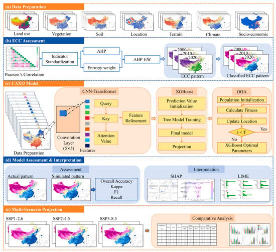
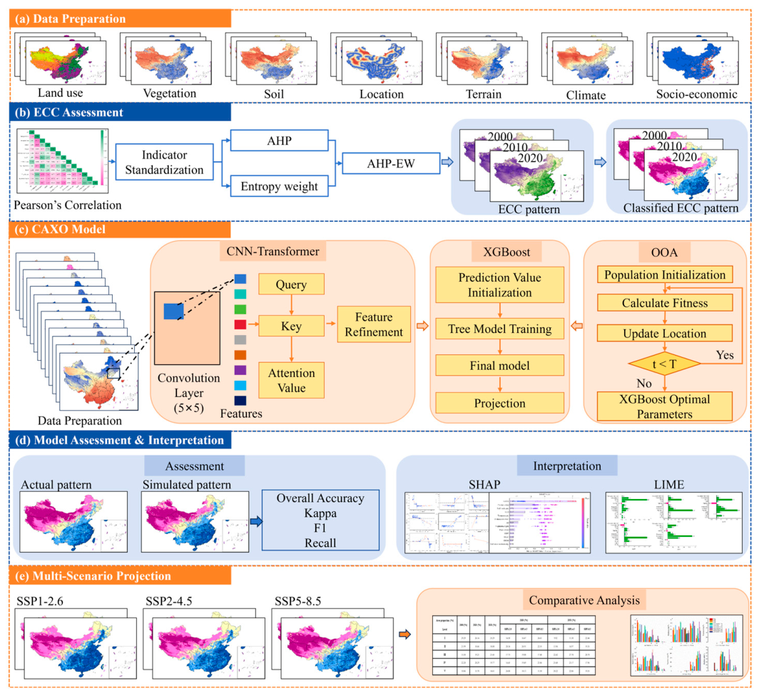
The workflow of this study comprises five components, as shown in Figure 1: (1) Data Preparation: To develop a comprehensive ECC evaluation system, we selected a diverse set of indicators from multiple domains, such as land use, vegetation, soil, location, terrain, climate, and socio-economic factors. (2) ECC Assessment: Initial indicators were refined by removing those exhibiting a Pearson correlation coefficient greater than 0.80 in order to reduce multicollinearity. Following this, the finalized indicators were standardized and integrated using AHP-EW weights to generate ECC evaluation results for 2000–2020. These results were then classified to identify spatiotemporal change patterns. (3) CAXO Model: The ECC assessment indicators and results served as input data for model training. Feature extraction was performed using a CNN–Transformer model. The extracted features were then input into the XGBoost model for training. We used the Osprey Optimization Algorithm (OOA) to optimize the XGBoost hyperparameters, which enhanced the model’s predictive accuracy. (4) Model Assessment and Interpretation: The predictive accuracy of the CAXO model concerning China’s ECC was rigorously assessed. Concurrently, interpretability analyses were conducted utilizing SHAP and LIME to elucidate the underlying factors influencing model projections. (5) Multi-Scenario Projection: We projected distribution patterns of ECC in China for 2030 and 2050 based on commonly used SSP scenarios and conducted relevant analyses. Based on the observed spatial and temporal dynamics, targeted recommendations for ecological conservation were formulated.
Figure 1.
The workflow for ECC assessment and ECC projection based on the CAXO model.
2.2. AHP-EW Model
For the ECC evaluation method, we adopted the AHP-EW model from previous research to assign weights to the indicators [24]. This method merges the Analytic Hierarchy Process (AHP) and Entropy Weighting (EW) to create a composite weighting model. It combines subjective judgments with objective data, overcoming the limitations of individual methods.
2.3. CAXO Model
The CAXO model is an integrated framework with three modules. It works as follows: The local spatial features of the data are first extracted using a Convolutional Neural Network (CNN). Subsequently, the self-attention mechanism of the Transformer is employed to uncover long-range spatio-temporal dependencies, thereby generating high-dimensional spatio-temporal fusion features. The osprey optimization algorithm (OOA) then optimizes the hyperparameters of the XGBoost model, which ultimately generates ECC projection results using the weighted features and optimized parameters. The model can be given by:
where denotes the predicted vector of ECC; represents the ensemble projection function derived from the XGBoost model; is the weight matrix of the core self-attention mechanism in the Transformer computed based on query, key, and value; is the local features extracted by a convolutional neural network from the spatiotemporal input indicator matrix, where denotes the number of samples, t denotes the historical time step, and denotes the number of indicators; and is the set of XGBoost hyperparameters optimized by OOA.
The CNN–Transformer model mitigates metric redundancy and addresses the challenge of capturing nonlinear relationships between metrics in traditional feature selection by extracting key features from raw indicators and assigning weights [25]. This module of the CNN–Transformer model uses a parallel single-indicator feature extractor and self-attention weight allocation to reveal deep features across metrics. It starts with batch normalization to address dimensional differences and data fluctuations. Then, multiple rounds of convolution and activation operations apply a sliding window for weighted summation, uncovering internal correlation features within each indicator [26]. The formula for this convolutional operation can be given by [27]:
where denotes the batch-normalized value of the jth metric at the ith sample for the tth time step; is the raw value of the jth metric at the ith sample for the tth time step; and are the learnable scaling and offset factors for batch normalization; is the mean of the jth metric; is the variance of the jth metric; and is a small constant (typically set to 10−5) to prevent division by zero. denotes the output of the jth feature of the ith sample after convolution at the tth time step; represents the ReLU activation function; denotes the convolution kernel size; is the batch-normalized value of the (j + k)th feature in the ith sample at the tth time step; is the weight at the kth position of the convolution kernel; and is the bias term of the convolution layer. The features of each indicator are compressed to a uniform dimension after several convolutions. These extracted features are then concatenated to form , serving as input for the self-attention mechanism.
The self-attention mechanism module allocates weights by assessing the importance of indicators [28]. The CNN’s feature matrix is mapped to three vector spaces, creating three attention matrices [29]. The similarity between these matrices is computed and normalized into weights using the function. Finally, a weighted sum of the value vectors is performed to produce a refined feature representation. The calculation can be given by:
where is the normalization function; is the query matrix, where is the number of samples and denotes the attention dimension; is the transpose of the key matrix; and is the scaling factor to prevent gradient saturation.
Since XGBoost model has numerous parameters and is prone to getting stuck in local optima [30], we chose the OOA for global hyperparameter optimization. The OOA simulates the hunting behavior of ospreys by initially generating a population within a specified hyperparameter range [31]. During exploration, it mimics the osprey’s foraging, evaluates fitness to assess solution quality, and updates positions based on prey distribution to discover new search areas [23]. During the capture phase, the algorithm mimics an osprey adjusting its position after catching prey, conducting a fine search to improve the current solution. After several iterations, it outputs the optimal hyperparameter combination , finalizing the parameter optimization for the XGBoost model. The formulation of this algorithm can be given by [32]:
where is the jth hyperparameter of the ith individual, , , L is the dimension of the hyperparameters; and are the minimum and maximum values of the jth hyperparameter; is a uniform random number in the interval [0, 1]; represents the set of XGBoost hyperparameters (including tree depth, learning rate, regularization coefficient, etc.); and denotes the cross-validation error rate of the model under hyperparameters . A smaller fitness value indicates a more optimal combination of hyperparameters. is the new position of the jth dimension of the ith osprey in the first search phase; is the position of the fish selected by the ith osprey in the jth dimension; is a random real number uniformly drawn from the interval [1,2]. is the new position of the jth dimension of the ith osprey in the second stage; is the current iteration number, which gradually reduces the search step size to enhance local exploitation.
XGBoost achieves ensemble projection through optimized hyperparameters, with its core mechanism being the iterative training of multiple decision trees [33]. This process transforms the weak projections of individual trees into strong projections through ensemble integration [34]. The model parameter configuration corresponds to . During projection, each decision tree maps the input weighted features to its corresponding leaf node and outputs the node’s weight, calculated using the formula [35]:
where is the projection value of the tth tree for the ith sample; is the weighted feature matrix; is the weight of the leaf node belonging to the ith sample in the tth tree; and is the leaf node index of the ith sample in the tth tree.
The projections from all trees are ultimately aggregated using a learning rate-weighted summation, with the formula being [36]:
where is the final predicted category for sample i; is the total number of trees after OOA optimization; is the projection result that maximizes the function value within the parentheses; and is the learning rate after OOA optimization.
The CAXO model was implemented using Python 3.9 with TensorFlow 2.12 and Keras for the CNN–Transformer module, XGBoost 1.7 for the ensemble learning module, and the Osprey Optimization Algorithm coded in Python.
2.4. Model Assessment and Interpretation
To assess the predictive accuracy of the CAXO model, we employed OA, Kappa, F1, and recall metrics to reflect projection precision. The formulas are as follows [37,38]:
where is the number of samples correctly simulated; is the total number of samples; is the number of ECC levels; denotes the correct number of the ith ECC level in the simulation results; and denote the number of samples of the ith ECC level in the actual and simulated results; represents the number of samples that are genuinely classified as the target ECC level but are misclassified by the model as a non-target level; and is the number of samples that are actually not in the target ECC level but were incorrectly predicted to belong to that level.
After training the XGBoost model, to gain a deeper understanding of the model’s projection logic, we conducted post hoc attribution analysis using two methods: SHAP and LIME [39].
The SHAP method fairly distributes the difference between model projection and baseline projection across input features by calculating the weighted average of the marginal contribution of a specific feature across all possible feature subsets [40]. This formula can be given by [41]:
where denotes the contribution value of feature to the model projection for the current sample ; is the feature for which the SHAP value is being computed; is the complete set of all features; is a subset of the feature set ; denotes the number of features in the subset ; denotes the total number of features in the entire feature set ; represents the conditional expectation function of the model’s projection for sample given the feature subset ; and represents the conditional expectation of the model’s projection when feature is added to .
The LIME method approximates the behavior of complex models by constructing locally interpretable models near specific projection points [21]. It first generates a set of perturbed samples within the neighborhood of the target samples. Perturbed samples are predicted using the original model, and their similarity to the target sample is measured with a similarity kernel function, which can be given by [42]:
where is the similarity kernel function; is the distance function between the original sample and the perturbed sample ; and is the hyperparameter controlling the kernel width, which determines the size of the local neighborhood. The larger the value of , the higher the weight assigned to samples farther from , and the larger the local range becomes.
The optimization problem involves finding a simple and interpretable model that closely approximates the complex model in locally weighted neighborhoods defined by , while maintaining sparsity for better interpretability. This optimization objective can be given by the following formulation [43]:
where is the solution to the optimization problem; is the locally interpretable proxy model; is the total number of perturbed samples; is the similarity weight for sample ; is the projection for sample by the CAXO model; is the projection value given by the interpretable model for perturbation sample ; and is the complexity penalty of model . The weight vector from this problem provides a local interpretation for sample , indicating the importance and influence direction of each feature on the projection.
Accuracy assessment metrics (OA, Kappa, F1, recall) were calculated using Scikit-learn 1.2. SHAP and LIME interpretability analyses were performed using the SHAP 0.41 and LIME 0.2 packages in Python.
2.5. Scenario Downscaling Methodology
The future scenario data—including LULC, precipitation, temperature, GDP, and population for 2030 and 2050—are aligned with three SSP-RCP scenarios: SSP1-2.6 (low emissions, sustainable development), SSP2-4.5 (medium emissions, middle of the road), and SSP5-8.5 (high emissions, fossil-fueled development). The coupling between each variable and the SSP-RCP scenarios is as follows.
The climate variables come from CMIP6 multi-model ensemble outputs and are bias-corrected using the delta downscaling method [44]. For each SSP-RCP scenario, monthly anomalies are computed between future periods (2021–2040, 2041–2070, 2071–2100) and the historical baseline (1991–2020). These anomalies are calculated as absolute differences for temperature and relative differences for precipitation. They are then resampled to 1 km resolution via cubic spline interpolation and applied to high-resolution historical observations. The magnitude of change varies by scenario. By 2100, the annual mean temperature over China increases by 0.64 °C to 5.83 °C, with SSP5-8.5 showing the strongest warming and SSP1-2.6 the weakest [44].
The population projections are generated using a random forest framework that incorporates SSP-consistent built-up land data [45]. The model captures nonlinear relationships between population distribution and predictors such as slope, distance to city centers, distance to roads, distance to water, and built-up land. A recursive approach extends the gridded projections from 2010 to 2100 at ten-year intervals, with national and global population totals constrained by SSP assumptions. The three scenarios reflect different population trajectories: SSP1 features low population that peaks mid-century and then declines; SSP2 shows moderate growth; and SSP5 exhibits high, continuous growth.
The GDP projections are obtained from a global gridded GDP dataset consistent with the SSPs [46]. This dataset provides 1 km resolution GDP projections in 2005 PPP USD from 2030 to 2100 at ten-year intervals under all five SSP scenarios. The projections are generated using the LitPop downscaling approach, which combines nighttime light images (NPP-VIIRS for future periods) and gridded population data (LandScan) to disaggregate national and subnational GDP projections. National GDP projections under each SSP are taken from the OECD SSP database, with growth rates varying by scenario: lowest under SSP1, moderate under SSP2, and highest under SSP5. For China, the projections account for the two-child policy and use provincial-level GDP projections from Li et al [45]. The LitPop approach achieves high accuracy at the provincial scale (R2 = 0.97) and county scale (R2 = 0.80–0.90) [46].
The LULC projections are derived from a global SSP-RCP consistent dataset at 1 km resolution [47]. The dataset is produced by coupling the Global Change Assessment Model (GCAM) with the Patch-generating Land Use Simulation (PLUS) model. GCAM simulates LULC demands at the water-basin level (235 basins globally) under different SSP-RCP scenarios, accounting for variations in climate and socio-economic factors. The PLUS model then downscales these basin-level demands to 1 km by simulating patch-level changes across six land classes: cropland, forest, grassland, urban, barren, and water. The three SSP scenarios yield distinct patterns: SSP1-2.6 preserves forests and limits urban expansion; SSP2-4.5 shows moderate changes; and SSP5-8.5 exhibits rapid urban expansion at the expense of farmland and grassland. The dataset achieves high simulation accuracy (Kappa = 0.94, OA = 0.97) [47].
3. Study Area and Data Sources
3.1. Study Area
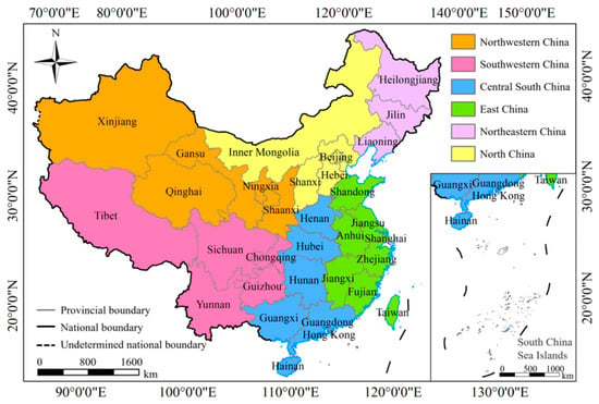
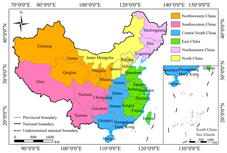
China is in eastern Asia along the western Pacific coast. The total land area is approximately 9.6 million square kilometers [48]. The region features three distinct terraces, including the Qinghai–Xizang Plateau, the Tarim Basin, and the Yangtze Plain. This varied terrain leads to diverse climatic zones, ranging from the humid monsoon areas in the southeast to arid regions in the northwest and the cold climate of the Qinghai–Xizang Plateau. From a comprehensive geographical perspective, China is usually divided into six major regions: North China, Northeast China, East China, Central South China, Southwest China, and Northwest China (Figure 2). Each region has unique characteristics regarding natural topography, climatic conditions, economic development, and cultural patterns, which together contribute to the overall diversity of China’s geographical environment.
Figure 2.
Overlay map of China’s provincial administrative divisions and geographical zones within the study area. Note that Figure 2 is based on the standard map (GS(2024)0650) of the Standard Map Service (bzdt.ch.mnr.gov.cn), and the base map has not been modified.
As the world’s second-largest economy and most populous nation, China is undergoing rapid industrialization and urbanization, with an urbanization rate now exceeding 66% [49]. Rapid urban development has created high-density economic zones but has also stressed the ecological environment. Coastal areas face issues like water scarcity and soil contamination, while central and western regions deal with soil erosion and desertification. The tension between economic development and environmental protection is growing increasingly evident. This study aims to develop a methodology to evaluate the ECC of various regions in China and predict future trends. The results will assist in creating targeted environmental protection policies and fostering a balance between economic and ecological development.
3.2. Datasets and Preprocessing
Table 1 summarizes data sources for ECC assessment and projection. Land use data were obtained from the China Multi-period Land Use Remote Sensing Monitoring Dataset (CNLUCC) [50]. MOD13A3 data were utilized to obtain annual average NDVI values to explore the relationship between ECC and vegetation [51]. Soil moisture data were obtained from the Global Daily Surface Soil Moisture dataset at 1 km resolution (2000–2020) released by the National Qinghai-Tibet Plateau Scientific Data Center [52]. Soil erosion data were sourced from the Scientific Data Bank—these data cover the years 2000, 2010, and 2020 and have a spatial resolution of 1000 m [53].
Table 1.
Data sources for ECC evaluation indicators.
Location data was sourced from the National Catalogue Service for Geographic Information to study river influence on ECC [54]. The DEM was obtained from NASA, and the slope was calculated using ArcMap10.8. Precipitation and temperature data came from historical records at the Resource and Environmental Science Data Center. AI was derived from NASA MOD16A2 [55]. Nighttime light data for 2000, 2010, and 2020 were acquired from DMSP-OLS and NPP-VIIRS [56,57]. GDP and population data for these years were provided by the Resource and Environment Science Data Center [58,59]. All MODIS data underwent reprojection and formatting using the MODIS Reprojection Tool (MRT).
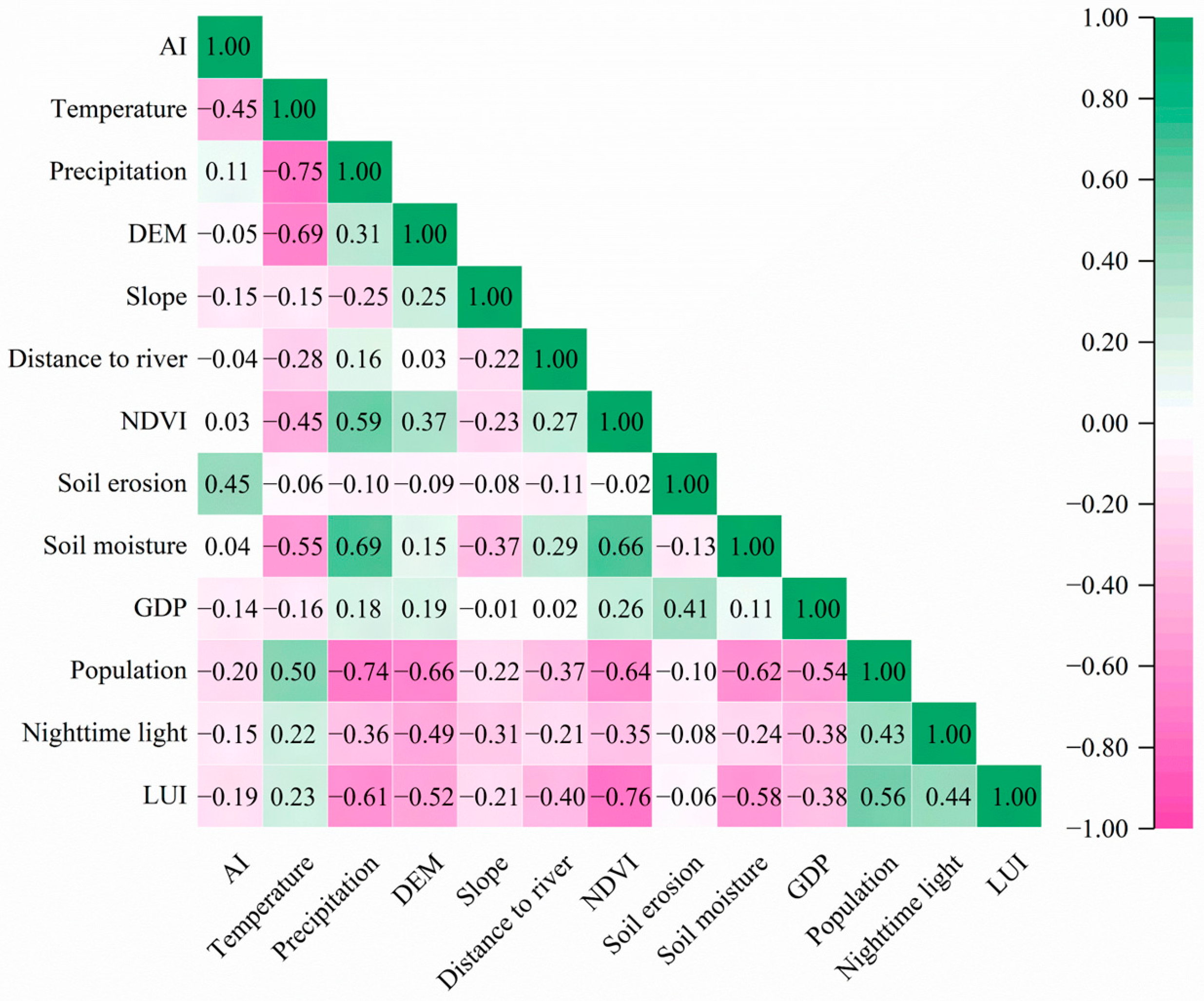
As shown in Figure 3, the correlation coefficients among the indicators are below 80%, indicating they are not highly correlated and independently represent ECC without information overlap [60]. It also demonstrates that the ECC evaluation indicator system constructed in this study exhibits good independence, which is capable of reflecting regional ECC from multiple dimensions and laying a foundation for the reliability of subsequent assessment results.
Figure 3.
Heatmap of Pearson correlation coefficients for screening ECC evaluation indicators.
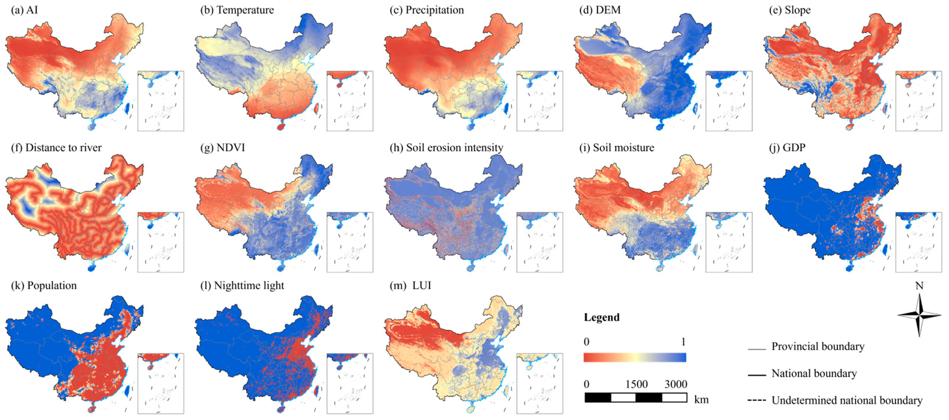
Figure 4 details the thirteen indicators selected for the ECC assessment, specifically including AI, temperature, precipitation, DEM, slope, distance to rivers, NDVI, soil erosion intensity, soil moisture, GDP, population, nighttime light, and LUI. Given the differing dimensional units and wide numerical ranges of these indicators, direct application in analysis risks scale interference. Therefore, all indicators underwent Min-Max normalization. This process effectively eliminated the impact of dimensional units and numerical ranges while preserving the original discrete characteristics of each indicator.
Figure 4.
Evaluation indicators for ECC.
4. Results
4.1. ECC Distribution Pattern for 2000–2020
The ECC evaluation indicators were normalized, and AHP-EW weights were calculated. The weighting results are shown in Table 2. Among these weights, the highest values were assigned to AI (0.16), precipitation (0.16), and NDVI (0.13), indicating that these three factors exert the greatest influence on ECC. GDP (0.09) and population (0.09) followed closely, with moderate influence on the ECC model; soil erosion intensity (0.01) had the lowest weight.
Table 2.
Weights of ECC evaluation indicators.
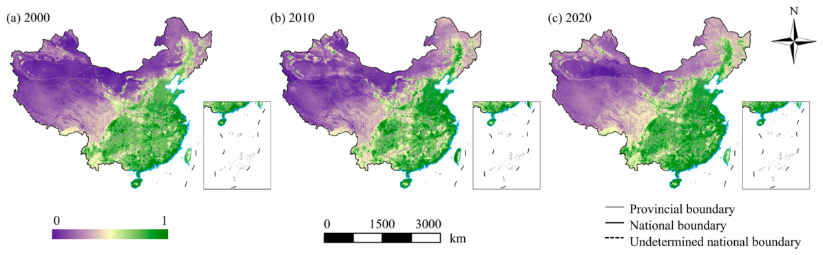
Through weighted calculations based on thirteen indicators, the ECC patterns for China in 2000, 2010, and 2020 were ultimately obtained (Figure 5). Overall, ECC values tend to be higher in southeastern China, while western regions exhibit lower ECC values. Combining the distribution evolution from 2000 (Figure 5a), 2010 (Figure 5b), and 2020 (Figure 5c), the extent and intensity of high-value areas showed an expanding trend, most notably in the northeast, while low-value areas exhibited a shrinking trend.
Figure 5.
ECC evaluation patterns of China in 2000, 2010, and 2020.
To more intuitively illustrate the interannual variations of ECC, we have categorized ECC values into five levels, using 0.2 as the interval. These levels correspond to poor, fair, medium, good, and excellent ECC conditions, respectively, as shown in Table 3.
Table 3.
ECC Criteria for Classification in China.
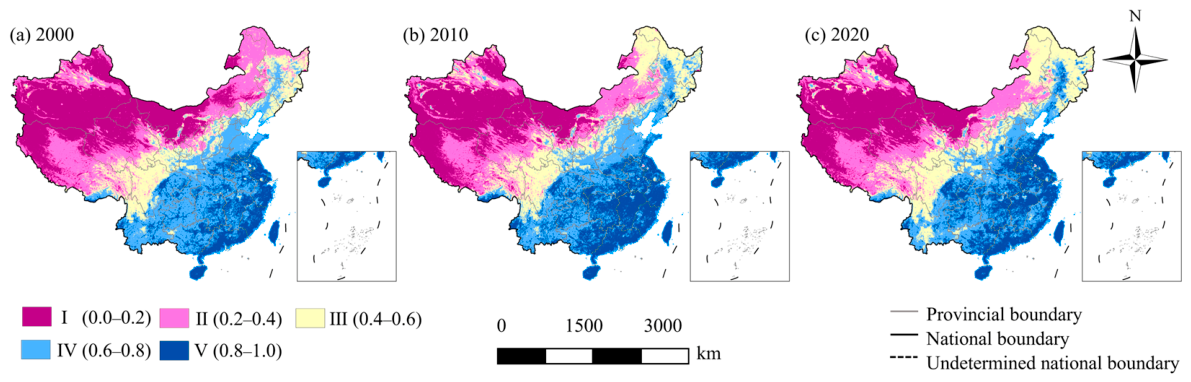
We used the reclassify tool in ArcMap to classify the ECC patterns, ultimately obtaining classified ECC patterns for China in 2000, 2010, and 2020. Figure 6 displays the five-level distribution maps of China’s ECC for these three years, revealing more pronounced distribution characteristics and trends compared to the ECC patterns (c.f. Figure 5). It is evident that the spatial patterns of ECC exhibit significant differences demarcated by the Hu Huanyong Line [61]: Level I and Level II (the most severe levels) are concentrated in the region west of the Hu Huanyong Line, Level III (moderate level) is primarily distributed around the Hu Huanyong Line, and Level V (best level) is concentrated in the region east of the Hu Huanyong Line.
Figure 6.
China’s ECC classified patterns in 2000, 2010, and 2020.
4.2. CAXO Model Training
To ensure the CAXO model accurately simulates and reproduces historical ECC patterns, calibration with optimal XGBoost parameters is required. Given the large number of parameters and complex tuning logic of XGBoost models, this experiment focuses on 10 core parameters for debugging. Corresponding value ranges are set for each parameter as boundary conditions for subsequent optimization, with specific parameters and ranges shown in Table 4.
Table 4.
XGBoost parameter ranges and final configuration.
During parameter optimization, the maximum number of iterations for the XGBoost model was preset to 1000. Additionally, to ensure optimal search performance of the OOA, experimental validation was conducted on the initial population size. Its value range was constrained to [200, 1600], evaluation results of model simulation accuracy under different initial population sizes are presented in Table 5. When the population size was 1200, the model achieved optimal performance, with an overall accuracy of 90.01%, a Kappa coefficient of 87.11%, an F1 score of 89.45%, and a recall rate of 89.14%. The final model parameters are also summarized in Table 4.
Table 5.
Accuracy of CAXO model’s simulation results under different population sizes.
4.3. Accuracy Assessment
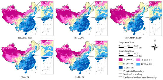
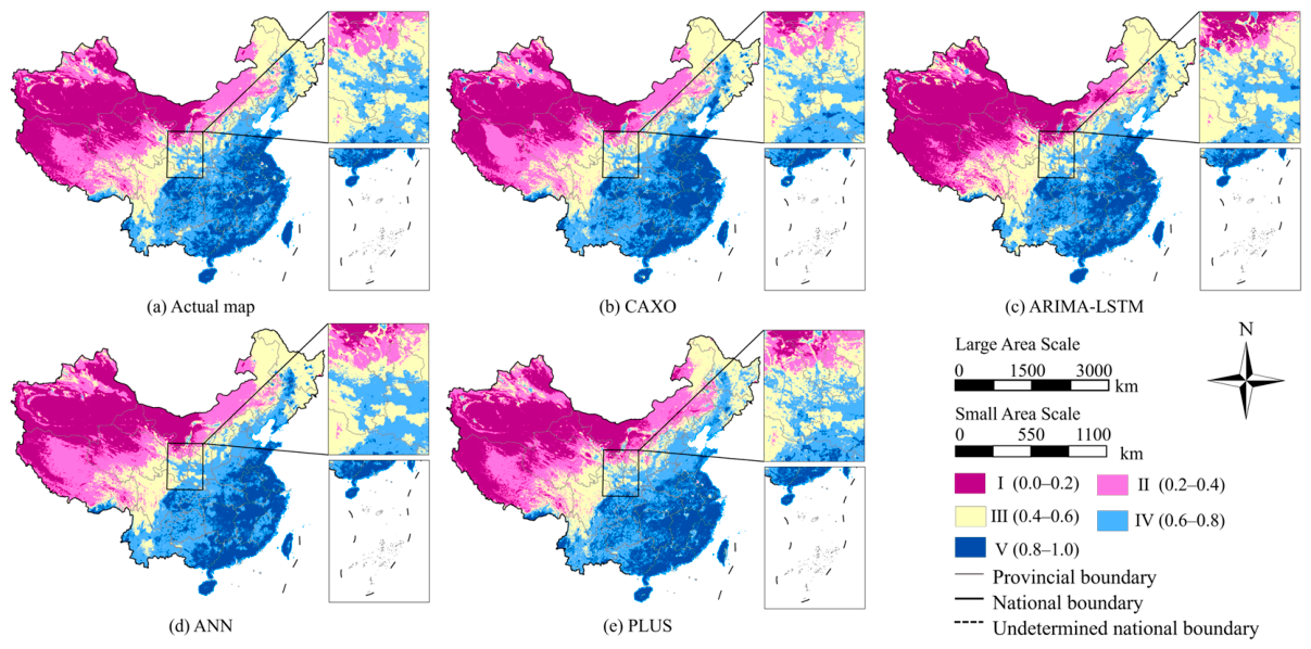
To more thoroughly validate the predictive accuracy of the CAXO model, we incorporated three established models from existing literature for comparative experiments. Specifically, the 2020 ECC patterns simulated by all four models were compared with the actual 2020 ECC patterns. The specific comparison results are shown in Figure 7.
Figure 7.
China’s ECC actual map and four model simulation maps in 2020.
Figure 7 shows that compared to the 2020 ECC actual map, the CAXO model simulated results (Figure 7b) more closely match the ECC actual map (Figure 7a). In the ARIMA-LSTM simulation map (Figure 7c), local enlargements reveal that the predicted range for level I ECC significantly exceeds the actual extent. Additionally, the edge contours of level III ECC differ from those on the ECC actual map, with a broader overall distribution. The ANN simulation map centers on level III ECC (Figure 7d), where its edge details appear relatively coarse, especially in smaller areas of the map. The PLUS model’s deviation primarily manifests in level V ECC (Figure 7e), where the predicted number far exceeds that on the ECC actual map.
Additionally, we evaluated the accuracy of these models, with results shown in Table 6. As indicated in the table, the CAXO model exhibits the highest simulation accuracy, followed by ARIMA-LSTM. We further compared CAXO with ARIMA-LSTM, which is the second most accurate model, and found CAXO achieved improvements across four core metrics. These metrics include 2.24% in OA, 2.22% in Kappa, 0.97% in F1 score, and 1.63% in Recall. This further demonstrates the CAXO model’s superior predictive accuracy and reliability in ECC pattern simulation. Although the numerical improvement in overall accuracy appears modest, Figure 7b clearly shows that the spatial distribution of each ECC level simulated by CAXO more closely resembles the actual ECC pattern than the other three models, an advantage that aggregate metrics alone cannot capture. Moreover, for practical applications such as ecological redline delineation, spatial coherence is often more important than marginal gains in overall accuracy.
Table 6.
Model’s accuracy assessment and improvement of CAXO over ARIMA-LSTM.
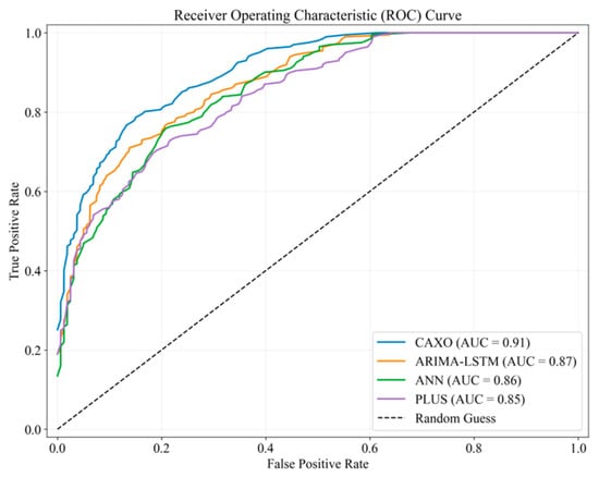
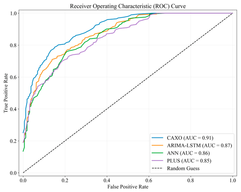
We further evaluated model performance from a discriminative ability perspective, with results presented via ROC (Receiver Operating Characteristic) curves in Figure 8. Among the four models, the CAXO model ranked first with an Area Under the Curve (AUC) of 0.91. Its ROC curve lies closest to the upper-left corner of the coordinate system, indicating the strongest ability to distinguish positive and negative samples. The ARIMA-LSTM (0.87) followed closely behind; the classification performance of the ANN (0.86) and the PLUS (0.85) decreased successively. In summary, the CAXO model achieves optimal classification accuracy and reliability in ECC pattern simulation and projection tasks.
Figure 8.
ROC curves for CAXO, ARIMA-LSTM, ANN, and PLUS models.
4.4. SHAP Global Feature Interpretation
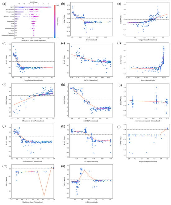
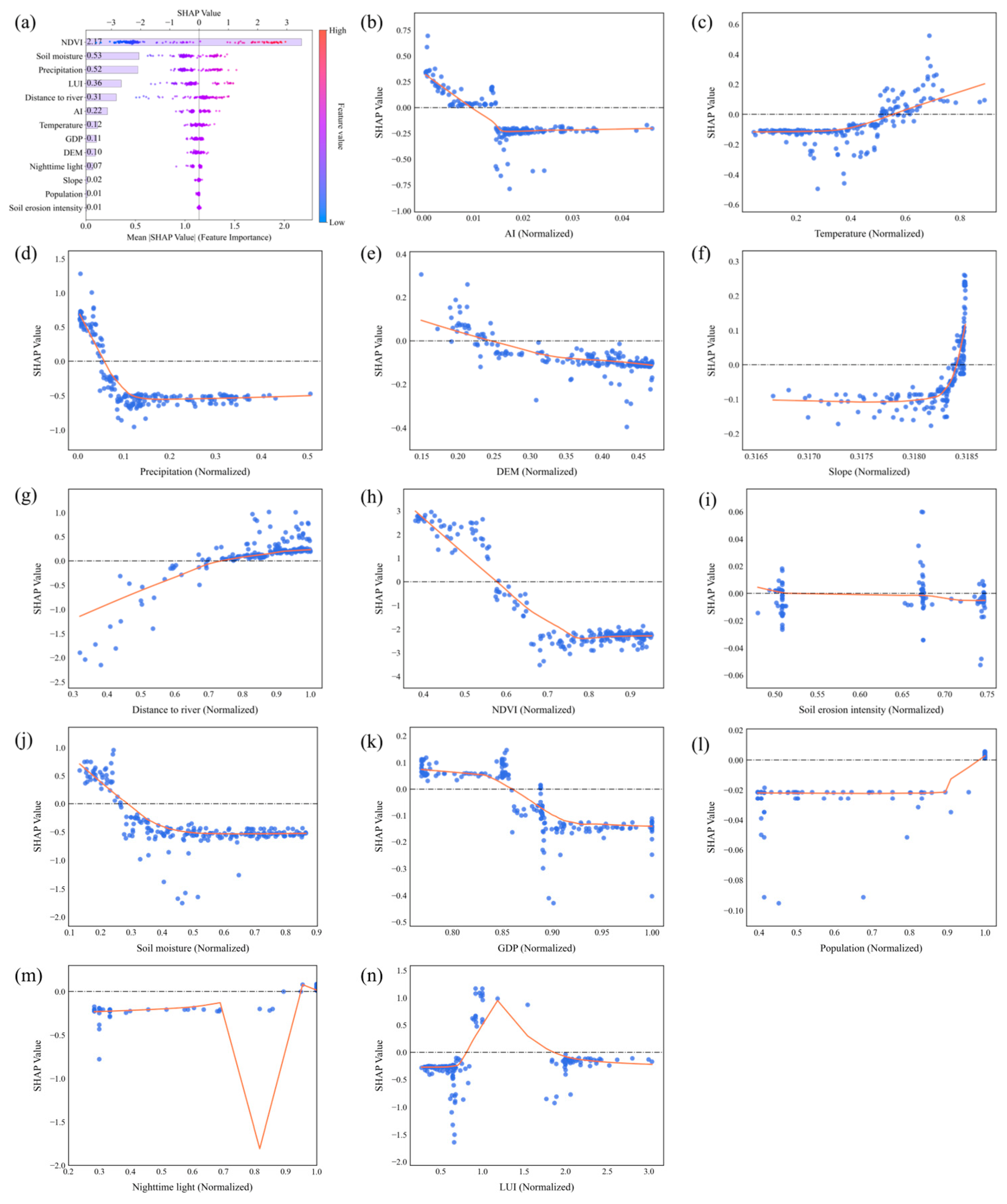
To investigate the feature importance and marginal contribution of CAXO model in ECC projection, this study employs the SHAP method for global interpretation. Figure 9a displays the feature importance ranking and summary overlay results, where NDVI (2.17), soil moisture (0.53), and precipitation (0.52) exert the most significant influence on model outputs. The higher SHAP mean values of these three features indicate that vegetation status and moisture conditions are the core factors determining ECC.
Figure 9.
SHAP feature importance and feature dependency plots for the CAXO model. (a) SHAP summary plot, where the horizontal axis represents the SHAP value, the color indicates the feature value (blue for low, red for high), and the bar on the right shows the feature importance; (b–n) SHAP dependence plots for each driving factor, where the horizontal axis is the normalized feature value, the vertical axis is the corresponding SHAP value, the orange line represents the trend of SHAP values with the feature value, and the dashed line indicates a SHAP value of zero.
The SHAP dependency analysis in Figure 9b–n reveals the complex nonlinear effects of various drivers on ECC. The declining trend of AI normalization values within the 0–0.01 range indicates drought constrains ECC, while rising temperatures exhibit a pronounced promoting effect. Precipitation exhibits a positive influence at low values, with diminishing marginal benefits beyond a threshold. A critical threshold occurs at slope values below 0.32, where human activity pressure induces negative effects; above this threshold, improved soil conservation shifts the impact to positive. Increasing distance from rivers significantly enhances ecological functions, reflecting gradient changes in human disturbance. NDVI shows a negative correlation with ECC, potentially because the relatively monotonous ecosystem structure in areas with high vegetation coverage leads to insufficient diversity and stability of their ecological service functions. Soil moisture turns negative beyond 0.30, suggesting root hypoxia in overly wet conditions. GDP growth shifts from promoting to inhibiting beyond a specific threshold, reflecting environmental pressures from economic expansion. Nighttime light promotes ecological function within the 0.20–0.70 range but declines significantly beyond 0.70, indicating the positive effects of moderate human activity. Land use intensity also exhibits an optimal range, where moderate development enhances ECC through resource optimization.
4.5. LIME Local Interpretation
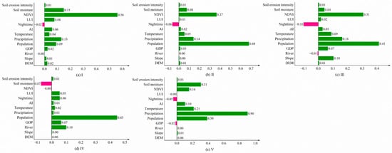
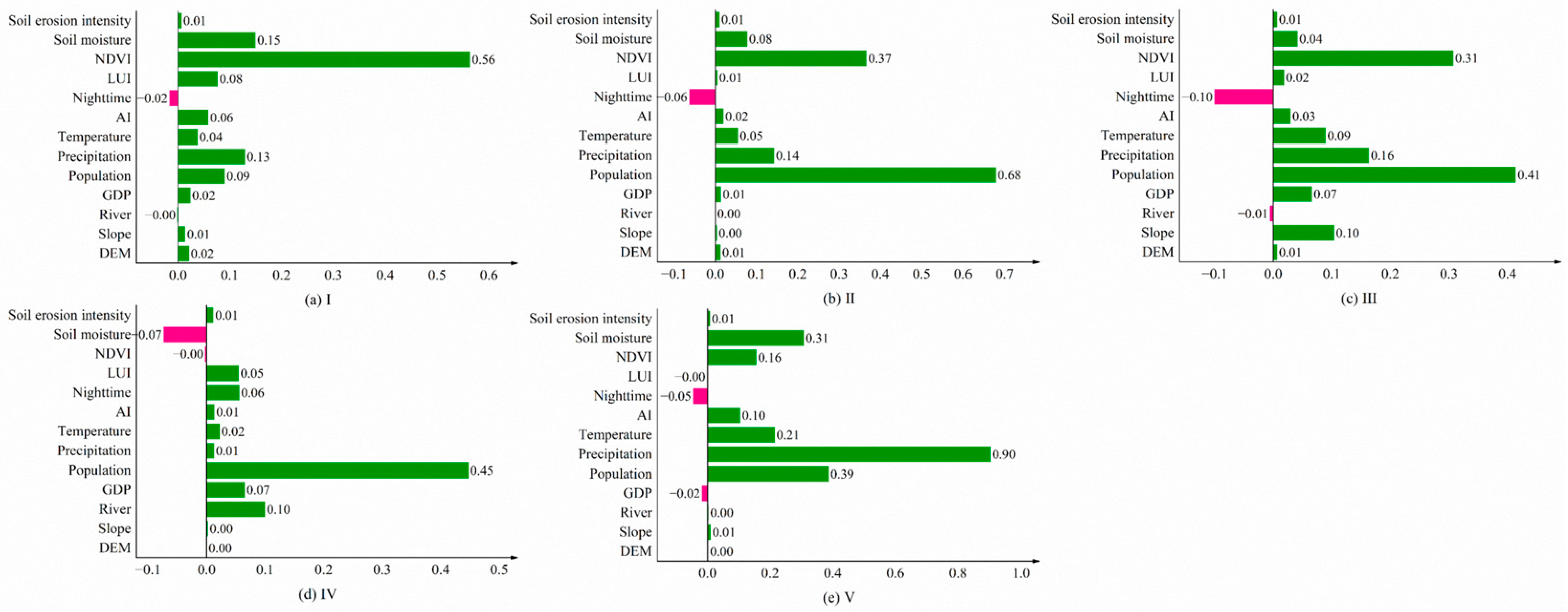
We employed the LIME method for interpretive analysis to analyze the predictive logic of the CAXO model for the five ECC levels from a local perspective. As shown in Figure 10, the contribution characteristics of different ECC levels exhibit significant differences, fundamentally reflecting the dynamic equilibrium between ecological supply capacity and human disturbance intensity.
Figure 10.
Feature importance of LIME under different ECC levels. Green bars indicate positive contributions to feature importance, while red bars indicate negative contributions.
Level I (Figure 10a) represents the minimal ecological carrying capacity, maintained solely by modest positive influences from NDVI (0.56) and soil moisture (0.15). This condition is characterized by high vulnerability, where even slight perturbations from nighttime light (−0.02) can disrupt this delicate balance. In level II (Figure 10b), population density (0.68) and NDVI (0.37) support ecological functions, but human resource consumption approaches its upper limit, with nighttime light pollution (−0.06) exacerbating ecological degradation. Level III (Figure 10c) relies on population (0.41), NDVI (0.31), and precipitation (0.16) for foundational support. Nighttime illumination (−0.10) and river distance (−0.01) begin to suppress carrying capacity, maintaining ecological conditions at a moderate level. Level IV (Figure 10d) maintains a high ECC level despite minor impacts on soil moisture (−0.07), as human activities remain within thresholds and river resources are efficiently utilized (river distance shows a positive contribution of 0.10). Level V (Figure 10e) achieves stable and healthy ECC through peak precipitation contributions (0.90) and positive effects from population (0.39) and soil moisture (0.31), coupled with minimal human disturbance (nighttime light: −0.05, GDP: −0.02).
Overall, as ECC levels increase, the dominant positive contributing factors gradually shift from NDVI and soil moisture to a state centered on precipitation and supported by multiple synergistic factors. Although the negative impacts of human disturbances (such as nighttime light and GDP) persist, their intensity diminishes relative to the increasingly robust ecological supply capacity. This fully confirms the pivotal role of the dynamic equilibrium between ecological supply and human activities in determining ECC levels.
4.6. Scenario Projection
Given the high accuracy of the CAXO projection model, we conducted multi-scenario projection of China’s ECC for 2030 and 2050 based on different scenarios from Shared Socioeconomic Pathways (SSP) coupled with Representative Concentration Pathways (RCP). The parameter standards for these SSP-RCP scenarios are provided in Supplementary Material S1. Specifically, SSP1-2.6 refers to low greenhouse gas emission pathways for sustainable development. SSP2-4.5 reflects balanced socioeconomic development with moderate emissions. SSP5-8.5 represents high-emission scenarios characterized by intensive fossil fuel consumption and rapid economic growth.
Table 7 shows a clear gradient of change across the three scenarios. SSP5-8.5, the high-emission pathway, leads to the most pronounced changes: temperature rises by 2.28 °C, GDP increases by 49.50 trillion USD, and urban land expands by 9.8%. In contrast, SSP1-2.6, the sustainable pathway, results in the smallest warming (1.30 °C) and the largest forest expansion (6.50%). SSP2-4.5 shows moderate changes across all variables, falling between the other two scenarios. The projected spatial distributions of ECC under the three scenarios are shown in Figure 11.
Table 7.
Statistical changes in key variables under three SSP-RCP scenarios (2020–2050) [44,45,46,47].
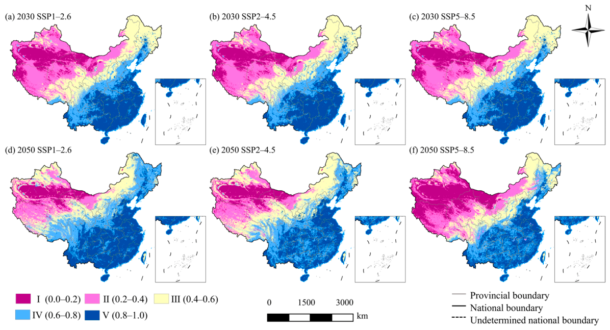
Figure 11.
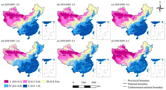
ECC patterns in China for 2030 and 2050 under three SSP-RCP scenarios based on CAXO model projection.
From 2030 to 2050, under the low-emission sustainable scenario SSP1-2.6 (Figure 11a,d), regions with high ECC (levels IV and V) significantly expand, particularly in North China and Northeast China, where ECC markedly improves by 2050. Under the medium-emission scenario SSP2-4.5 (Figure 11b,e), ECC shows limited improvement while regional disparities widen. Under the high-emission SSP5-8.5 scenario (Figure 11c,f), areas with low ECC (levels I and II) substantially expand, with severe ecological degradation occurring in Northwest China and North China by 2050. Concurrently, higher emissions and more extensive development lead to weaker ECC, with this disparity between scenarios becoming more pronounced by 2050 compared to 2030.
We conducted statistical analysis on historical and projected ECC data to understand ECC trends. Results are presented in Table 8. From a historical perspective (2000–2020), China’s ECC demonstrates an overall positive development trend, primarily reflected in the continuous reduction in low-level areas and the steady expansion of high-level areas. The proportions of ECC Level I and Level II areas decreased from 29.29% and 21.99% to 25.29% and 18.88%, respectively, indicating a gradual reduction in ecologically vulnerable zones. The proportion of Level V areas increased from 10.86% to 14.61%, demonstrating significant conservation achievements in ecologically sound regions. This shift primarily resulted from a series of national ecological conservation and restoration initiatives implemented during this period, coupled with reduced resource consumption driven by socioeconomic restructuring.
Table 8.
Statistics on the proportion of China’s ECC areas by level in 2000, 2010, 2020, and under three SSP-RCP Scenarios for 2030 and 2050.
For future multi-scenario projection, under the low-emission sustainable development pathway SSP1-2.6, the proportion of Level V regions is projected to increase to 28.22% by 2050, while Level I regions will decrease to 9.92%, highlighting the significant synergistic effects of low-carbon transition and ecological conservation. Under the high-emission SSP5-8.5 scenario, an extensive development model characterized by high-intensity resource consumption will intensify ecological pressures. By 2050, Level I areas are projected to account for 22.44%, with ecosystems facing degradation risks. Meanwhile, under the medium-emission SSP2-4.5 pathway, ecological conservation and restoration achievements remain relatively limited due to balanced social development and emission levels without breakthrough improvements.
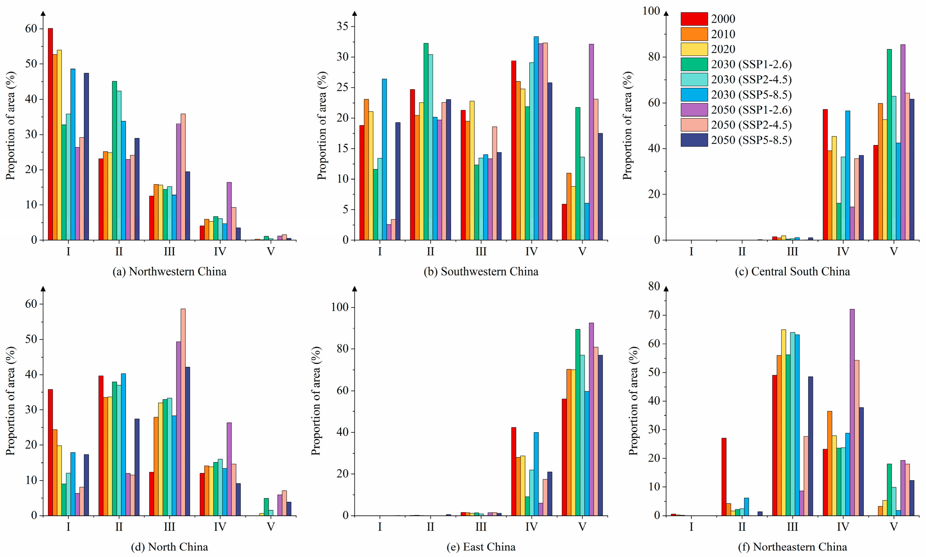
To investigate the spatiotemporal characteristics and scenario responses of ECC at the regional scale, we conducted a statistical analysis of the proportion of ECC area across six major regions in China: Northwestern China, Southwestern China, Central South China, North China, East China, and Northeastern China. The results are shown in Figure 12.
Figure 12.
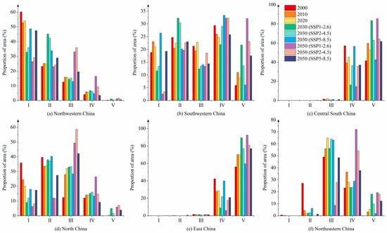
Area proportion of ECC levels under six geographical subdivisions in 2000, 2010, 2020, and under three SSP-RCP scenarios in 2030 and 2050.
Northwest China (Figure 11a) shows a drop in level I ECC area proportion from 60.15% (2000) to 53.96% (2020); projections will reach 26.35% (SSP1-2.6) and 47.47% (SSP5-8.5) by 2050, requiring prioritized ecological water security. Southwest China (Figure 11b) shows a rise in level I areas from 18.77% (2000) to 21.05% (2020), while level V will likely be boosted to 32.15% under SSP1-2.6, calling for geological hazard prevention. Central South China (Figure 11c) shows an increase in level V from 41.43% (2000) to 52.70% (2020) and will likely retain 61.65% under SSP5-8.5 by 2050, needing forest ecosystem protection. North China (Figure 11d) shows a decrease in level I from 35.88% (2000) to 19.81% (2020), and level I will be lowered to 6.31% under SSP1-2.6 by 2050, requiring groundwater remediation. East China (Figure 11e) shows a rise in level V from 55.97% (2000) to 70.07% (2020), and level V is projected to hit 92.65% under SSP1-2.6 by 2050. Northeast China (Figure 11f) shows a shift from dominant level III (49.07%, 2000) to medium–high levels (2020), and level IV will account for 72.14% under SSP1-2.6 by 2050 through forest conservation.
5. Discussions
5.1. Selection of ECC Projection Model
ECC is the outcome of long-term interaction between the supply capacity of natural ecosystems and the intensity of human disturbance. Its projection must address core challenges, including the heterogeneity of multi-source data, nonlinear relationships among factors, and spatiotemporal dynamic evolution. When dealing with complex systems, traditional single models often struggle to balance the efficiency of multi-factor integration simultaneously, the ability to identify critical information, and the stability of projection accuracy.
Traditional models such as ARIMA-LSTM and ANN operate on a pixel-wise basis, where each grid cell is predicted independently using only its own temporal trajectory [62]. This approach lacks awareness of surrounding neighborhood information. When adjacent pixels exhibit slight data variations due to original noise or interpolation errors, the model may assign them to different ECC levels, resulting in blurred boundaries and fragmented patches. As shown in Figure 7c, the ARIMA-LSTM prediction displays poorly defined Level III boundaries that differ markedly from the actual map. In Figure 7d, the ANN model produces scattered small patches for Levels III, IV, and V, failing to form coherent ecological zones. The CNN module in CAXO applies convolutional kernels over local windows, integrating neighborhood context during feature extraction [25,26]. This effectively smooths out data anomalies in individual pixels, yielding contiguous patches and clearly defined boundaries (Figure 7b).
ECC is driven by multiple interacting factors whose relative importance varies spatially and across ECC levels. Fixed-weight approaches cannot capture this context dependency. The self-attention mechanism in Transformer dynamically computes attention scores for each indicator based on the input data, allowing the model to emphasize water-related factors in arid zones and socioeconomic factors in urban clusters [19,63]. Meanwhile, SHAP analysis of the trained CAXO model (Figure 9) confirms that NDVI, soil moisture, and precipitation are the globally dominant drivers, while also revealing heterogeneous factor contributions across different ECC levels [40].
XGBoost contains numerous hyperparameters whose settings significantly affect predictive performance. Manual tuning is time-consuming and prone to suboptimal local minima [30]. The Osprey Optimization Algorithm mimics the hunting behavior of ospreys—global exploration followed by local exploitation—to efficiently search the hyperparameter space [64]. As shown in Table 5, OOA converged to an optimal configuration at a population size of 1200, achieving 90.01% overall accuracy. XGBoost employs a gradient-boosting framework that iteratively builds an ensemble of decision trees, with each new tree correcting the errors of its predecessors [65]. This mechanism handles mixed data types, resists overfitting, and captures nonlinear relationships among ECC drivers [14,22].
These four components form a coherent pipeline: CNN extracts local spatial features and mitigates the boundary blurring and patch fragmentation caused by pixel-wise prediction; Transformer assigns context-aware dynamic weights; OOA automatically optimizes model hyperparameters; and XGBoost generates the final ensemble prediction. This integration explains why CAXO not only achieves higher overall accuracy but also produces spatially coherent ECC maps with well-defined boundaries. Furthermore, the embedded SHAP and LIME interpretability modules transform CAXO from a purely predictive tool into a diagnostic one, capable of revealing the mechanistic drivers behind ECC dynamics.
5.2. Integration of Model Interpretability Methods
As machine learning models grow more complex in ecological forecasting, their “black box” nature poses a significant challenge. This characteristic stems from an inability to explain the mechanisms behind their projections, making it difficult to apply these advanced models in practical ecological management [66]. In this context, integrating interpretability methods becomes essential for developing ecological models that achieve both predictive accuracy and operational transparency.
SHAP provides a global perspective on model behavior, identifying key features and their directional influences [16]. Based on game theory, SHAP calculates each feature’s contribution to every projection and aggregates these effects across the dataset [67]. As shown in Figure 9a, this approach confirms NDVI, soil moisture, and precipitation as primary drivers of ECC in our CAXO model. More importantly, the dependency plots in Figure 9b–n reveal nonlinear relationships and threshold effects between these features and ECC projections. This allows us to understand not just which factors matter, but how they matter—specifically, how their effects change across different value ranges.
LIME complements this global view with local explanations. It constructs simple interpretable models that approximate the complex model’s behavior around specific instances [17]. Our analysis of five ECC levels (Figure 10) shows that feature contributions vary significantly across ecological contexts. For example, population density functions as a stressor in low-ECC areas but becomes supportive in high-ECC regions. This demonstrates our model’s ability to capture context-dependent relationships rather than simple linear effects.
The integration of SHAP and LIME creates a synergistic effect. SHAP offers a macro-view of feature importance, albeit potentially oversmoothed, while LIME provides a micro-view of decision logic for single instances, despite its localized scope [18]. By combining these top-down and bottom-up perspectives, this study enables mutual validation between the identification of core drivers and their mode of operation across hierarchical ECC levels. This synergy strengthens confidence in the model’s decision process and offers a rigorous methodological foundation for deriving ecological insight from predictive outputs. Therefore, the systematic integration of SHAP and LIME holds significant methodological value for modeling ECC and other complex environmental systems.
5.3. Suggestions
Based on this study of ECC, while some progress has been made, significant room for optimization remains. Based on research into ECC, while some progress has been made, there remains significant room for optimization. A unified ECC evaluation system struggles to accommodate regional ecological heterogeneity. Research indicates that while 13 universal indicators can characterize ECC from multiple dimensions, they cannot precisely match the core ecological constraints of different regions. Therefore, it is recommended to establish a hierarchical evaluation framework combining universal indicators with region-specific indicators. National unified core indicators such as NDVI and precipitation should be adopted to ensure comparability across regional ECC assessments. Simultaneously, differentiated indicators should be configured for distinct regional ecological baselines. Arid zones should prioritize assessments of water resource carrying capacity, land desertification, and soil salinization levels, while urban clusters should focus on urban green space coverage and heat island effect intensity. This approach reveals common characteristics of overall ECC at the macro level while precisely identifying core ecological issues in each region. Consequently, it provides more accurate scientific support for ecological conservation efforts, emphasizing differentiated guidance and region-specific policies.
For constructing the CAXO projection model, we introduced a feature attention mechanism to optimize weight allocation but failed to incorporate spatial context. This led the model to overlook water-related factors (e.g., soil moisture, precipitation) when processing arid region data and socioeconomic factors (e.g., nighttime light, GDP) when analyzing eastern urban clusters, ultimately compromising the accuracy of identifying ECC driving mechanisms across regions. We therefore recommend improving the model’s feature weight allocation logic by compressing CNN-extracted spatial feature maps into scene description vectors via global pooling and inputting these alongside original structured features into the attention network. This achieves dynamic binding between feature weights and spatial context. For instance, the system automatically elevates water-related feature weights when processing northwest data and emphasizes human activity-related features when analyzing urban clusters. This enhances the model’s adaptability to regional ecological characteristics, strengthens the scientific validity of dominant factor identification, and further improves ECC projection accuracy.
Based on the ECC projection results under different scenarios and the statistical analysis results of each region, the following ecological protection recommendations are proposed. At the regional governance level, implement differentiated protection strategies. In the northwest region, prioritize the development of water-saving irrigation technologies to enhance agricultural water use efficiency; in the southwest region, undertake karst landscape restoration and establish a geological hazard monitoring network; in North China, promote industrial water recycling and water-saving agriculture; and in Central South China, construct urban–rural ecological networks to mitigate the urban heat island effect through green space development and ventilation corridor planning. At the policy assurance level, establish an industry access system based on carrying capacity assessments. Implement development restrictions in ecologically fragile areas while encouraging ecological industries in stable regions. Governments should integrate ECC indicators into performance evaluations to shift from reactive governance to proactive prevention and control. This new management mechanism provides institutional safeguards for achieving harmonious coexistence between humanity and nature.
6. Conclusions
We assessed ECC using the AHP-EW model and conducted multi-scenario projections using the CAXO model. Based on the ECC assessment, we observed a distinct ECC spatial distribution pattern of “high in the southeast, low in the northwest” for China from 2000 to 2020. The overall ecological condition for China improved, with areas classified as level V increasing from 10.86% to 14.61%. The CAXO model demonstrated 90.01% accuracy in ECC projections, significantly outperforming traditional models. Key factors influencing ECC projections include NDVI, precipitation, and soil moisture, with human activities showing a pronounced threshold effect. Projections for 2050 indicate that under the sustainable SSP1-2.6 pathway, high-capacity regions could rise to 28.22%, whereas under the high-emission SSP5-8.5 pathway, low-capacity areas could increase to 22.44%.
This study confirms the positive trend in China’s ECC while underscoring how development pathways impact ecosystems. It highlights the need for green transformation and tailored ecological governance to achieve sustainable development.
Supplementary Materials
The following supporting information can be downloaded at: https://www.mdpi.com/article/10.3390/rs18111690/s1. Table S1: Key parameter standards for SSP-RCP scenarios. SSP-RCP scenario definitions and key parameter standards used in this study. The Shared Socioeconomic Pathways (SSP) coupled with Representative Concentration Pathways (RCP) follow the standard definitions from the Intergovernmental Panel on Climate Change (IPCC) Sixth Assessment Report (AR6) [68].
Author Contributions
Conceptualization and methodology, X.T. and F.L.; formal analysis, data curation, and writing—original draft, F.L.; writing—review and editing, X.T.; visualization, F.L. and J.F.; supervision, X.T.; project administration and funding acquisition, X.T. All authors have read and agreed to the published version of the manuscript.
Funding
This research was funded by the National Natural Science Foundation of China (Grant No. 42561065) and the Natural Science Foundation of Xinjiang Uygur Autonomous Region (Grant No. 2023D01C31).
Data Availability Statement
The data presented in this study are available upon reasonable request, to be provided by the corresponding author.
Acknowledgments
We would like to thank all those who indirectly supported this study through their contributions to the field of ecology and environmental science.
Conflicts of Interest
The authors declare that they have no known competing financial interests.
References
- Xiong, J.; Wang, X.; Zhao, D.; Wang, J. Spatiotemporal evolution for early warning of ecological carrying capacity during the urbanization process in the Dongting Lake area, China. Ecol. Inform. 2023, 75, 102071. [Google Scholar] [CrossRef] [Scilit]
- Zhu, Y.H.; Chen, M.S.; Pan, M.Y.; Ren, Z.Y. Beyond funding: How income inequality shapes international clean energy finance’s influence on ecological carrying capacity in 114 developing countries. J. Environ. Manag. 2025, 393, 127045. [Google Scholar] [CrossRef] [Scilit]
- Gemitzi, A. Predicting land cover changes using a CA Markov model under different shared socioeconomic pathways in Greece. Giscience Remote Sens. 2021, 58, 425–441. [Google Scholar] [CrossRef] [Scilit]
- Yuan, S.; Liu, Y.; Liu, Y.; Zhang, K.; Li, Y.; Enwer, R.; Li, Y.; Hu, Q. Spatiotemporal variations of surface albedo in Central Asia and its influencing factors and confirmatory path analysis during the 21st century. Int. J. Appl. Earth Obs. Geoinf. 2024, 134, 104233. [Google Scholar] [CrossRef] [Scilit]
- Tang, Z.; Wu, Z.; Jia, X.; Liu, X.; Pei, X.; Liu, Z.; Xiong, X.; Li, J.; Liu, X.; Wu, C.; et al. Nationwide occurrence of emerging benzophenone, benzotriazole, salicylate and triazine ultraviolet filters in coastal sediment of China: Spatial distribution, source and ecological risk. Environ. Res. 2025, 287, 123140. [Google Scholar] [CrossRef] [Scilit]
- Duo, L.; Wang, J.; Zhang, F.; Xia, Y.; Xiao, S.; He, B.-J. Assessing the Spatiotemporal Evolution and Drivers of Ecological Environment Quality Using an Enhanced Remote Sensing Ecological Index in Lanzhou City, China. Remote Sens. 2023, 15, 4704. [Google Scholar] [CrossRef] [Scilit]
- Hartley, T. Is carrying capacity useful for integrating humans into Earth system models? On the purposes and limits of modelling. Ecol. Model. 2025, 508, 111232. [Google Scholar] [CrossRef] [Scilit]
- Paz, A.; Lauber, T.; Crowther, T.W.; van den Hoogen, J. Improving access and use of climate projections for ecological research through the use of a new Python tool. Ecography 2024, 2024, e07186. [Google Scholar] [CrossRef] [Scilit]
- Xu, P. Prediction of Per Capita Ecological Carrying Capacity Based on ARIMA-LSTM in Tourism Ecological Footprint Big Data. Sci. Program. 2022, 2022, 6012998. [Google Scholar] [CrossRef] [Scilit]
- Zhang, Z.; Jiang, W.; Xiao, Z.; Ling, Z.; Sun, J.; Song, J.; Li, X. Optimal simulation of future restoration and protection spatial for mangroves and assessment of disaster prevention and mitigation functions with SDG13.1. J. Clean. Prod. 2025, 516, 145784. [Google Scholar] [CrossRef] [Scilit]
- Ji, W.; Wang, Z.; Zhang, H.; Zhang, B.; Yang, F.; Yu, Z.; Li, H.; He, M.; Lv, H.; Feng, Z. Carbon storage change, driving mechanism, and scenario prediction in Beijing-Tianjin-Hebei region for regional carbon neutral target: From history to future. Sci. Total Environ. 2025, 993, 180028. [Google Scholar] [CrossRef] [Scilit]
- Damdin, B.; Lantuu, U.; Avirmed, B.; Bayaraa, B.; Natsagdorj, E. Predicting fodder crop yield in semi-arid Mongolia using Landsat data: A multivariate analysis approach. Can. J. Remote Sens. 2025, 51, 2564877. [Google Scholar] [CrossRef] [Scilit]
- Schiller, J.; Stiller, S.; Ryo, M. Artificial intelligence in environmental and Earth system sciences: Explainability and trustworthiness. Artif. Intell. Rev. 2025, 58, 316. [Google Scholar] [CrossRef] [Scilit]
- Liu, Y.H.; She, J.J.; Wang, L.; Li, Z.J.; Guo, Z.H. Decoding urban flood resilience in the Henan section of the Yellow River Basin: Insights from an XGBoost-SHAP analysis. J. Environ. Manag. 2025, 394, 127632. [Google Scholar] [CrossRef] [Scilit] [PubMed]
- Ganie, S.M.; Pramanik, P.K.D.; Zhao, Z. Lifestyle data-based multiclass obesity prediction with interpretable ensemble models incorporating SHAP and LIME analysis. Sci. Rep. 2025, 15, 36916. [Google Scholar] [CrossRef] [Scilit]
- Afzali, S.A.E.; Shayanfar, M.A.; Ghanooni-Bagha, M.; Golafshani, E.; Ngo, T. The use of machine learning techniques to investigate the properties of metakaolin-based geopolymer concrete. J. Clean. Prod. 2024, 446, 141305. [Google Scholar] [CrossRef] [Scilit]
- Saadatfar, H.; Kiani-Zadegan, Z.; Ghahremani-Nezhad, B. US-LIME: Increasing fidelity in LIME using uncertainty sampling on tabular data. Neurocomputing 2024, 597, 127969. [Google Scholar] [CrossRef] [Scilit]
- Schulte, L.; Ledel, B.; Herbold, S. Studying the explanations for the automated prediction of bug and non-bug issues using LIME and SHAP. Empir. Softw. Eng. 2024, 29, 93. [Google Scholar] [CrossRef] [Scilit]
- Hasan, H.; Garcia, M.A.; Rashwan, H.; Puig, D. CoHAtNet: An integrated convolutional-transformer architecture with hybrid self-attention for end-to-end camera localization. Image Vis. Comput. 2025, 162, 105674. [Google Scholar] [CrossRef] [Scilit]
- Kim, S.; Jung, J.; Lee, K.J. A Real-Time Sparsity-Aware 3D-CNN Processor for Mobile Hand Gesture Recognition. IEEE Trans. Circuits Syst. I-Regul. Pap. 2024, 71, 3695–3707. [Google Scholar] [CrossRef] [Scilit]
- Devanathan, B.; Varshitha, K.J.; Kumar, L.P.; Lakshmanan, S.A.; Prakash, N.K. Explainable AI Framework Using XGBoost With SHAP and LIME for Multi-Scale Household Energy Forecasting. IEEE Access 2025, 13, 149750–149764. [Google Scholar] [CrossRef] [Scilit]
- Khan, S.; Juvigny-Khenafou, N.P.D.; Dalu, T.; Milham, P.J.; Hamid, Y.; Eltohamy, K.M.; Ullah, H.; Amiri, B.J.; Chen, H.; Wu, N. The influence of pH and temperature on benthic chlorophyll-a: Insights from SHAP-XGBoost and random forest models. Ecol. Inform. 2025, 91, 103355. [Google Scholar] [CrossRef] [Scilit]
- Alkhonaini, M.A.; Aljaffan, N.; Said, Y.; Alsamri, J.; Nemri, N.; Obayya, M.; Alzubaidi, A.A.; Alsariera, Y.A.; Alnfiai, M.M. Leveraging osprey optimization algorithm with deep ensemble learning for cybersecurity in CPS environment. Ain Shams Eng. J. 2025, 16, 103612. [Google Scholar] [CrossRef] [Scilit]
- Tang, X.; Liu, F.; Hu, X.; Feng, J. Assessment of Ecological Carrying Capacity and Spatiotemporal Evolution Analysis for Arid Areas Based on the AHP-EW Model: A Case Study of Urumqi, China. Land 2025, 14, 1143. [Google Scholar] [CrossRef] [Scilit]
- Liang, J.; Gao, Y. Lightweight memory-driven self-attention for hyperspectral image classification with CNN-transformer cross-feature fusion. Neurocomputing 2025, 651, 130998. [Google Scholar] [CrossRef] [Scilit]
- Nanni, L.; Lumini, A.; Barcellona, L.; Ghidoni, S. Convolutional neural networks and vision transformers for Plankton Classification. Ecol. Inform. 2025, 90, 103272. [Google Scholar] [CrossRef] [Scilit]
- Widneh, M.A.; Alemu, A.A.; Getie, D.D. Exploring Batch Normalization’s Impact on Dense Layers of Multiclass and Multilabel Classifiers. Int. J. Intell. Syst. 2025, 2025, 1466655. [Google Scholar] [CrossRef] [Scilit]
- Priyadharshini, S.; Bhoopalan, R.; Manikandan, D.; Ramaswamy, K. A successive framework for brain tumor interpretation using Yolo variants. Sci. Rep. 2025, 15, 27973. [Google Scholar] [CrossRef] [Scilit]
- Rahman, S.; Motiur Rahman, M.; Faezipour, M.; Rastgaar, M.; Ridelman, E.; Klein, J.D.; Angst, B.A.; Shanti, C.M. Enhancing Burn Severity Assessment With Deep Learning: A Comparative Analysis and Computational Efficiency Evaluation. Ieee Access 2024, 12, 147249–147268. [Google Scholar] [CrossRef] [Scilit]
- Ruggeri, D.; Vidacs, L. Advancing Wheat Single-Nucleotide Polymorphism Data Analysis with Explainable Deep Learning Models. Appl. Artif. Intell. 2025, 39, 2565169. [Google Scholar] [CrossRef] [Scilit]
- Al Duhayyim, M. Internet of things enabled indoor activity monitoring for visually impaired people with hybrid deep learning and optimized algorithms for enhanced safety. Sci. Rep. 2025, 15, 35438. [Google Scholar] [CrossRef] [Scilit] [PubMed]
- Khamies, M.; Fathy, A.; Hashem, M.; Alnuman, H.; Ali, H.H. A new methodology for optimal penetration of multiple type distributed generators based on large-scale unbalanced power distribution network. Eng. Sci. Technol.-Int. J.-Jestech 2025, 70, 102183. [Google Scholar] [CrossRef] [Scilit]
- Li, C.; Guo, S.; Huang, Q.; Mu, H.; Yuan, B.; Xia, Z.; Fang, H.; Zhang, W.; Tang, P.; Du, P. Dynamic monitoring of fine-grained ecological vulnerability in dryland urban agglomeration integrating novel remote sensing index and explainable machine learning. Giscience Remote Sens. 2025, 62, 2528302. [Google Scholar] [CrossRef] [Scilit]
- Nzabonantuma, L.; Nduwayezu, G.; Naghibi, A.; Nilsson, E.; Wali, U.G.; Larson, M. Flood susceptibility mapping in the Nyabarongo Catchment, Rwanda, based on data analysis and modeling. Geomat. Nat. Hazards Risk 2025, 16, 2556987. [Google Scholar] [CrossRef] [Scilit]
- Razavi-Termeh, S.V.; Sadeghi-Niaraki, A.; Ali, F.; Pirasteh, S.; Choi, S.-M. Particulate matter pollution prone-areas mapping using an enhanced explainable ensemble meta-algorithm. Int. J. Digit. Earth 2025, 18, 2557511. [Google Scholar] [CrossRef]
- Alwathaf, Y.; Al-Areeq, A.M.; Al-Masnay, Y.A.; Al-Aizari, A.R.; Al-Areeq, N.M. Enhancing flood susceptibility mapping in Sana’a, Yemen with random forest and eXtreme gradient boosting algorithms. Geocarto Int. 2025, 40, 2482707. [Google Scholar] [CrossRef] [Scilit]
- Faouzi, E.; Arioua, A.; Namous, M.; Barakat, A.; Mosaid, H.; Ismaili, M.; Eloudi, H.; Houmma, I.H. Spatial mapping of hydrologic soil groups using machine learning in the Mediterranean region. Catena 2023, 232, 107364. [Google Scholar] [CrossRef] [Scilit]
- Gui, S.; Li, J.; Chen, G.; Zhao, J.; Tang, B.; Li, L. Identification of Abandoned Cropland and Global-Local Driving Mechanism Analysis via Multi-Source Remote Sensing Data and Multi-Objective Optimization. Remote Sens. 2025, 17, 3086. [Google Scholar] [CrossRef] [Scilit]
- Ahmed, I.; Brahmacharimayum, A.; Ali, R.H.; Khan, T.A.; Ahmad, M.O. Explainable AI for Depression Detection and Severity Classification From Activity Data: Development and Evaluation Study of an Interpretable Framework. JMIR Ment. Health 2025, 12, e72038. [Google Scholar] [CrossRef] [Scilit]
- Zhang, J.Y.; Ma, X.L.; Zhang, J.L.; Sun, D.L.; Zhou, X.Z.; Mi, C.L.; Wen, H.J. Insights into geospatial heterogeneity of landslide susceptibility based on the SHAP-XGBoost model. J. Environ. Manag. 2023, 332, 117357. [Google Scholar] [CrossRef] [Scilit]
- Hamedianfar, A.; Maanavilja, L.; Sutinen, H. Evaluating ensemble machine learning and feature optimization for mapping peatland vegetation using UAS-derived data. Int. J. Appl. Earth Obs. Geoinf. 2025, 144, 104901. [Google Scholar] [CrossRef] [Scilit]
- Alabi, R.O.; Elmusrati, M.; Leivo, I.; Almangush, A.; Maekitie, A.A. Machine learning explainability in nasopharyngeal cancer survival using LIME and SHAP. Sci. Rep. 2023, 13, 8984. [Google Scholar] [CrossRef] [Scilit]
- Marin Diaz, G. A Fuzzy-XAI Framework for Customer Segmentation and Risk Detection: Integrating RFM, 2-Tuple Modeling, and Strategic Scoring. Mathematics 2025, 13, 2141. [Google Scholar] [CrossRef] [Scilit]
- Hu, X.; Shi, S.; Zhou, B.; Ni, J. A 1 km monthly dataset of historical and future climate changes over China. Sci. Data 2025, 12, 436. [Google Scholar] [CrossRef] [Scilit] [PubMed]
- Li, M.; Zhou, B.-B.; Gao, M.; Chen, Y.; Hao, M.; Hu, G.; Li, X. Spatiotemporal dynamics of global population and heat exposure (2020–2100): Based on improved SSP-consistent population projections. Environ. Res. Lett. 2022, 17, 094007. [Google Scholar] [CrossRef] [Scilit]
- Wang, T.; Sun, F. Global gridded GDP data set consistent with the shared socioeconomic pathways. Sci. Data 2022, 9, 221. [Google Scholar] [CrossRef] [Scilit]
- Zhang, T.; Cheng, C.; Wu, X. Mapping the spatial heterogeneity of global land use and land cover from 2020 to 2100 at a 1 km resolution. Sci. Data 2023, 10, 748. [Google Scholar] [CrossRef] [Scilit] [PubMed]
- Huang, X.; He, Y.; Xu, H.; Shen, Y.; Pan, X.; Wu, J.; Chen, K. Association between sociodemographic status and the T2DM-related risks in China: Implication for reducing T2DM disease burden. Front. Public Health 2024, 11, 1297203. [Google Scholar] [CrossRef] [Scilit]
- Fan, J.; Wang, J.; Qiu, J.; Li, N. Stage effects of energy consumption and carbon emissions in the process of urbanization: Evidence from 30 provinces in China. Energy 2023, 276, 127655. [Google Scholar] [CrossRef] [Scilit]
- Yang, J.; Huang, X. The 30 m annual land cover dataset and its dynamics in China from 1990 to 2019. Earth Syst. Sci. Data 2021, 13, 3907–3925. [Google Scholar] [CrossRef] [Scilit]
- Didan, K. MOD13A3 MODIS/Terra Vegetation Indices Monthly L3 Global 1km SIN Grid V006; NASA Land Processes Distributed Active Archive Center: Sioux Falls, SD, USA, 2015. [Google Scholar] [CrossRef] [Scilit]
- Zheng, C.; Jia, L.; Zhao, T. A 21-year dataset (2000–2020) of gap-free global daily surface soil moisture at 1-km grid resolution. Sci. Data 2023, 10, 139. [Google Scholar] [CrossRef] [Scilit]
- Yan, J.; Wang, S.; Feng, J.; He, H.; Wang, L.; Sun, Z.; Zheng, C. New 30-m resolution dataset reveals declining soil erosion with regional increases across Chinese mainland (1990–2022). Remote Sens. Environ. 2025, 323, 114681. [Google Scholar] [CrossRef] [Scilit]
- National Catalogue Service for Geographic Information. 1:1,000,000 Public Version of Fundamental Geographic Information Data (2021). 2021. Available online: https://www.webmap.cn/commres.do?method=result100W (accessed on 14 November 2025).
- Running, S.M.; Mu, Q.; Zhao, M. MODIS/Terra Net Evapotranspiration 8-Day L4 Global 1km SIN Grid V006; NASA Land Processes Distributed Active Archive Center: Sioux Falls, SD, USA, 2017. [Google Scholar] [CrossRef]
- Ghosh, T.; Baugh, K.E.; Elvidge, C.D.; Zhizhin, M.; Poyda, A.; Hsu, F.-C. Extending the DMSP Nighttime Lights Time Series beyond 2013. Remote Sens. 2021, 13, 5004. [Google Scholar] [CrossRef] [Scilit]
- Elvidge, C.D.D.; Hsu, F.C.; Zhizhin, M.; Ghosh, T.; Sparks, T. Statistical moments of VIIRS night-time lights. Int. J. Remote Sens. 2024, 45, 7778–7802. [Google Scholar] [CrossRef] [Scilit]
- Xu, X.L. China GDP Spatial Distribution Kilometer Grid Dataset; Resource and Environment Science Data Registration and Publishing System, Institute of Geographic Sciences and Natural Resources Research, Chinese Academy of Sciences: Beijing, China, 2017. [Google Scholar] [CrossRef]
- Xu, X.L. China Population Spatial Distribution Kilometer Grid Dataset; Resource and Environment Science Data Registration and Publishing System, Institute of Geographic Sciences and Natural Resources Research, Chinese Academy of Sciences: Beijing, China, 2017. [Google Scholar] [CrossRef]
- Wu, X.; Huang, X. Screening of urban environmental vulnerability indicators based on coefficient of variation and anti-image correlation matrix method. Ecol. Indic. 2023, 150, 110196. [Google Scholar] [CrossRef] [Scilit]
- Ma, Z.; Xiao, H.; Li, J.; Chen, H.; Chen, W. Study on how the digital economy affects urban carbon emissions. Renew. Sustain. Energy Rev. 2025, 207, 114910. [Google Scholar] [CrossRef] [Scilit]
- Mahmud, A.; Noor, S.H.N.S.H.; Musa, K.I.; Hamzah, F.M.; Yudin, Z.M.; Kamaruddin, N.; Madawana, A.M.; Nawi, M.A.A. Hybrid ARIMA-LSTM for COVID-19 forecasting: A comparative AI modeling study. PeerJ Comput. Sci. 2025, 11, e3195. [Google Scholar] [CrossRef] [Scilit]
- Sa, J.; Ryu, J.; Kim, H. ECTFormer: An efficient Conv-Transformer model design for image recognition. Pattern Recognit. 2025, 159, 111092. [Google Scholar] [CrossRef] [Scilit]
- Hasanien, H.M.; Alsaleh, I.; Alassaf, A. Impact of electric vehicles and wave energy systems on OPF of power networks using hybrid Osprey-PSO approach. Energy 2024, 308, 132818. [Google Scholar] [CrossRef] [Scilit]
- Saghir, A.; Basit, R.; Lal, H.; Amjad, A.; Abdulfattah, O.; Shahbaz, K.M.; Tag, E.E.; Amin, N.M. The Deep Learning ResNet101 and Ensemble XGBoost Algorithm with Hyperparameters Optimization Accurately Predict the Lung Cancer. Appl. Artif. Intell. 2023, 37, 2166222. [Google Scholar] [CrossRef] [Scilit]
- Bello, M.; Napoles, G.; Concepcion, L.; Bello, R.; Mesejo, P.; Cordon, O. REPROT: Explaining the predictions of complex deep learning architectures for object detection through reducts of an image. Inf. Sci. 2024, 654, 119851. [Google Scholar] [CrossRef] [Scilit]
- Chung, C.-W.; Chou, S.-C.; Kao, C.-M.; Chen, Y.-J.; Hsiao, T.-H.; Chen, Y.-M. Application of machine learning algorithm for the prediction of lupus nephritis using SNP data, polygenic risk score, and electronic health record. Health Inform. J. 2025, 31, 14604582251363510. [Google Scholar] [CrossRef] [Scilit] [PubMed]
- Bongaarts, J. IPCC, 2023: Climate Change 2023: Synthesis Report. Contribution of Working Groups I, II and III to the Sixth Assessment Report of the Intergovernmental Panel on Climate Change; IPCC: Geneva, Switzerland, 2024. [Google Scholar] [CrossRef] [Scilit]

Disclaimer/Publisher’s Note: The statements, opinions and data contained in all publications are solely those of the individual author(s) and contributor(s) and not of MDPI and/or the editor(s). MDPI and/or the editor(s) disclaim responsibility for any injury to people or property resulting from any ideas, methods, instructions or products referred to in the content. |
© 2026 by the authors. Licensee MDPI, Basel, Switzerland. This article is an open access article distributed under the terms and conditions of the Creative Commons Attribution (CC BY) license.