A UAV Hyperspectral Inversion Framework for Mapping Soil Heavy Metals Based on Spectral Harmonization, Weighted Ensemble Learning, and Environmental Variable Integration

Highlights

What are the main findings?

• An interpretable UAV–laboratory synergistic framework integrating spectral harmonization, weighted ensemble learning, and environmental covariates successfully mapped soil Cd and Pb in an open-pit mining area, achieving the best predictive performance (R² = 0.85).
• SHAP and Grad-CAM analyses showed that Cd prediction was mainly associated with the 440–580 nm range and pH–SOM interactions, whereas Pb prediction was dominated by the 720–740 nm range and SOM–SMC coupling.

What are the implications of the main findings?

• The framework demonstrates that UAV hyperspectral inversion, when combined with spectral transfer correction and stable ensemble learning, can provide reliable and interpretable monitoring of soil heavy metals in complex mining environments.
• By linking UAV spectral observations with model-derived spectral responses and environmental associations through explainable AI, this study provides a practical and interpretable framework for Cd and Pb mapping, balancing predictive accuracy, model stability, and mechanistic interpretability.

Abstract

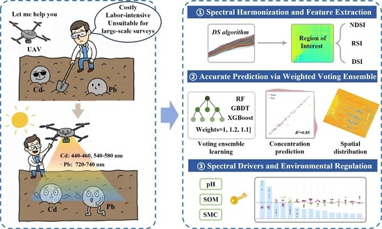
Accurate identification of HMs contamination in mine tailings is essential for understanding pollution and supporting remediation. However, conventional laboratory monitoring is labor-intensive, time-consuming, and spatially discontinuous, while UAV hyperspectral inversion is limited by spectral inconsistency, unstable performance under small-sample conditions, and insufficient interpretability. Here, we developed an interpretable UAV–laboratory synergistic framework for Cd and Pb mapping in the Yitong open-pit mine. Forty site-level soil samples, composited from 200 subsamples, were linked with UAV hyperspectral observations. Direct Standardization was used to harmonize UAV and laboratory spectra. A weighted voting ensemble (RF, GBDT, and XGBoost) achieved the best performance (R² = 0.85), outperforming the individual models and showing slightly higher stability than CNN (R² = 0.84). Environmental covariates (pH, SOM, SMC) revealed distinct metal-specific prediction patterns: Cd was mainly associated with pH–SOM interactions, whereas Pb was more strongly associated with SOM–SMC coupling. SHAP and Grad-CAM identified sensitive spectral regions, with Cd linked to the 440–580 nm range and Pb to the 720–740 nm range. Overall, this study provides an integrated framework that combines spectral transfer correction, stable multi-model inversion, and mechanism-oriented interpretability for HMs monitoring in complex mining environments.

1. Introduction

Soil contamination by heavy metals (HMs) has become a major environmental concern, particularly in regions affected by intensive mineral exploitation. In mining areas, long-term extraction, ore beneficiation, and tailings disposal can lead to the accumulation, mobilization, and redistribution of toxic elements such as Cd and Pb [1,2]. Because of their persistence, mobility, and bioaccumulative nature, these contaminants pose serious threats to ecosystem quality and human health, while also complicating post-mining restoration and environmental management [3,4]. Accurate characterization of HM contamination patterns is therefore essential for understanding pollution processes, identifying priority areas for remediation, and supporting effective management of mining-affected environments.

Conventional monitoring of soil HMs typically relies on geostatistical interpolation methods (e.g., Kriging) based on sparse field sampling and laboratory chemical analysis. Although these approaches provide high analytical accuracy, they are costly, labor-intensive, time-consuming, and spatially discontinuous, making them unsuitable for the large-scale and high-frequency assessments required for effective environmental management [5]. Hyperspectral remote sensing offers a promising alternative by integrating spatial and spectral information and capturing subtle spectral responses associated with interactions between HMs and soil constituents such as minerals and organic matter [6]. Satellite and airborne platforms have shown potential for regional-scale monitoring [7], but their coarse spatial resolution and fixed revisit cycles often fail to resolve the fine-scale heterogeneity typical of mining landscapes [8,9]. In contrast, UAV-mounted hyperspectral sensors provide centimeter-level spatial resolution, high operational flexibility, and on-demand data acquisition. These advantages allow UAVs to bridge the gap between point-based field measurements and broad-scale remote observations, enabling better characterization of spatially heterogeneous contamination in mining environments [10].

Despite these advantages, the practical application of UAV-based remote sensing is severely hindered by “signal-to-noise” challenges. Unlike controlled laboratory environments, field spectra acquired by UAVs are inevitably compromised by complex environmental interferences, including soil moisture heterogeneity, variable illumination geometry, atmospheric path radiance, and sensor noise [11,12]. These perturbations often mask the weak spectral responses characteristic of trace HMs, leading to poor model generalization and instability. Consequently, transforming noisy field spectra into “quasi-laboratory” quality data that reflects intrinsic soil properties remains a critical bottleneck. The Direct Standardization (DS) algorithm, a spectral transfer technique widely used in chemometrics, theoretically allows for the mathematical reconstruction of spectral information by establishing a transfer matrix between “slave” (UAV) and “master” (lab) instruments [13]. Although DS and related spectral-transfer methods have been applied to harmonize laboratory, field, satellite, and UAV spectra for soil-property estimation [14,15], their efficacy in harmonizing UAV hyperspectral imagery with laboratory ASD spectra in complex open-pit mining scenarios remains under-explored and warrants rigorous empirical validation.

However, translating the spatial advantages of UAV hyperspectral imagery into reliable soil HM inversion remains methodologically challenging. Recent studies have demonstrated the feasibility of integrating UAV hyperspectral imagery with spectral calibration and machine learning inversion for soil heavy-metal mapping in mining areas [16]. Nevertheless, under small-sample and high-dimensional spectral conditions, single models often struggle to capture complex nonlinear relationships [17], while existing ensemble studies mainly emphasize accuracy rather than prediction stability and learner complementarity [18]. In addition, although soil heavy-metal spectra are strongly influenced by environmental covariates such as pH, soil organic matter (SOM), and soil moisture content (SMC), previous studies have rarely examined their coupled effects on inversion performance explicitly [19,20]. Deep learning models such as convolutional neural networks (CNNs) offer strong feature extraction capabilities, but their decision-making processes often remain insufficiently interpretable in terms of physical and geochemical significance [21,22]. Therefore, the key challenge is not merely to confirm the feasibility of UAV-based heavy-metal prediction, but to develop an inversion framework that integrates accuracy, stability, and interpretability.

To address these technical and methodological gaps, this study develops a UAV–laboratory synergistic framework for soil heavy-metal inversion in complex mining environments. The aim is to improve the accuracy, robustness, and interpretability of HMs assessment and to provide a basis for targeted remediation and environmental management. The specific objectives are to: (1) apply the DS algorithm to achieve spectral data assimilation between UAV imagery and laboratory standards, constructing a high-fidelity feature dataset; (2) evaluate optimal machine learning base models to construct a weighted voting ensemble model, benchmarking it against a CNN to assess performance across accuracy and stability dimensions; (3) assess the effects of pH, SOM, and SMC on HMs prediction under different covariate coupling scenarios; and (4) interpret the spectral and environmental drivers of HMs inversion using SHAP and Grad-CAM.

2. Materials and Methods

2.1. Study Area

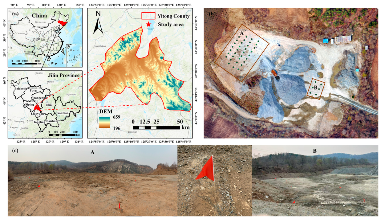
The study was conducted in a typical open-pit mining area in Yitong County, Jilin Province, China (Figure 1a). Located in the transitional area between the Changbai Mountains and the Songliao Plain, the region is characterized by gently undulating hilly terrain (Detailed environmental background information, including climate conditions, soil type, geological setting, and dominant land-cover characteristics, is provided in Appendix A.1).

Mining and mineral processing have long been the dominant economic activities in Yitong County, with the local industrial structure relying heavily on mineral resource exploitation that plays a critical role in regional economic development and local fiscal revenue. Similar to many mining cities in China, this prolonged dependence on resource extraction has imposed substantial environmental pressure [23], manifested by widespread exposed tailings and abandoned open pits resulting from decades of intensive mining activities (Figure 1b). Due to the lack of effective surface cover or containment measures, heavy metals in the tailings have been mobilized through rainfall leaching and surface runoff, subsequently accumulating in surrounding low-lying areas and forming a typical “source-sink” pollution pattern. To fully capture these pollution characteristics, the study area was divided into two sub-areas (Area A and Area B) (Figure 1c) with distinct micro-geomorphological features, covered by a sampling grid.

2.2. Data Acquisition: Synchronous Air-Ground Observation

Soil samples were collected in April 2025. Considering the spatial heterogeneity and pollution-source characteristics of the study area, a stratified sampling strategy was adopted. Area A (Figure 1b) contained the main exposed tailings, abandoned pits, and strongly disturbed mining surfaces, showing greater microtopographic and spectral heterogeneity. In contrast, Area B (Figure 1c) was a relatively smaller low-lying receiving area with more continuous surface conditions. A total of 40 sampling sites were distributed across the study area, including 34 sites in Area A and 6 sites in Area B. Surface soil (0–20 cm) was collected using a five-point sampling pattern [15,24], with one central point and four surrounding points located 1 m from the center. Thus, a total of 200 within-site subsamples were collected from 40 predefined sampling sites. The five subsamples within each site were composited to generate one representative site-level sample, resulting in 40 independent samples for laboratory analysis, UAV spectral matching, and subsequent modeling. Soil samples were air-dried, ground, sieved (100-mesh), and homogenized. Prior to analysis, the samples were digested using a hydrochloric–nitric–perchloric acid mixture, and heavy-metal concentrations (Zn, Cr, Cd, Pb, Ni) were determined via Inductively Coupled Plasma Atomic Emission Spectrometry (ICP-AES) [25].

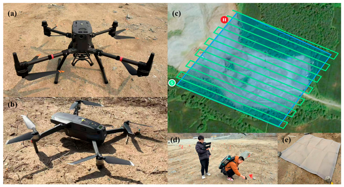
To ensure data consistency, the airborne campaign was conducted synchronously with ground sampling. A DJI M350 RTK quadrotor UAV, equipped with a Pika L hyperspectral camera, was deployed at a flight altitude of 100 m. The sensor acquired hyperspectral imagery spanning the 400–1000 nm range with a spectral resolution of 2.1 nm, providing detailed spectral signatures of the surface. Detailed sensor specifications and flight parameters are listed in Appendix A,

Table A1. Main technical details of hyperspectral camera and UAV.

Main Technical Details	Data
Spectral range	400–1000 nm
Spectral resolution	2.1 nm
Spectral channels	561
Spatial channels	900
Maximum frame rate	249 fps
Scanning frequency	320,000 points/s
UAV type	DJI M350 RTK

and

Table A2. Main technical details of flight parameters.

Main Flight Parameters	Data
Flight height	100 m
Flight speed	5 m/s
Time interval	1 ms
Field of view	17.6°
Side overlap	75%
Forward overlap	80%

. Prior to the mission, radiometric calibration was performed using a standard white reference panel placed within the study area to ensure spectral accuracy (Appendix A Figure A1e) [26]. The flight path was planned according to terrain characteristics (Appendix A Figure A1c), and the mission was executed under stable atmospheric conditions with a forward overlap exceeding 75% to guarantee seamless image stitching.

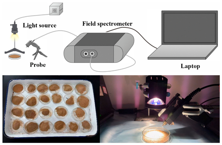
Given that in situ UAV imagery is susceptible to external perturbations—such as soil moisture heterogeneity, illumination variations, and atmospheric scattering—which can induce spectral distortion and mask intrinsic soil properties, laboratory measurements were conducted to establish a high-fidelity spectral baseline [27]. The reflectance spectra of all processed soil samples were acquired using an ASD FieldSpec3 portable spectroradiometer Analytical Spectral Devices, Inc, Boulder, CO, USA) in a controlled darkroom environment (Appendix A, Figure A2). This controlled setting eliminates environmental noise, ensuring the reliability of the “master” spectra used for subsequent calibration [28]. Detailed measurement protocols are outlined in Appendix A.2 of Appendix A.

2.3. Spectral Processing and Feature Engineering

2.3.1. UAV Image Preprocessing and Spectrum Extraction

The raw hyperspectral imagery was first subjected to geometric correction and cropping using MegaCube software (v2.7.0, IRIS, Inc., Beijing, China). Radiometric calibration was then performed using the Spectral on white reference panel to convert the raw image signal into relative reflectance. To ensure sub-meter spatial consistency, precise georeferencing was performed in ArcGIS 10.6, aided by high-resolution orthophotos. The processed image strips were subsequently mosaicked in ENVI (version 5.6, L3Harris Geospatial, Broomfield, CO, USA), where a 3 × 3 mean filter was applied to suppress pixel-level high-frequency sensor noise and enhance spatial continuity while providing mild spatial smoothing that preserves local surface heterogeneity at the sampling scale. Finally, pixel-level reflectance spectra corresponding to the 40 site-level sampling locations were extracted to form the spectral dataset used for subsequent spectral transfer and modeling.

2.3.2. Spectral Scale Transfer via Direct Standardization (DS)

UAV-acquired spectra were converted to relative reflectance through Spectral on white-reference calibration, which reduced radiometric inconsistencies and minimized part of the environmental noise. Nevertheless, residual discrepancies relative to laboratory reference measurements may still remain due to illumination geometry, atmospheric conditions, sensor characteristics, soil moisture, and observation-scale differences. To mitigate these discrepancies and assimilate the field spectra, the Direct Standardization (DS) algorithm was employed. DS functions by establishing a linear transfer matrix that maps the “slave” spectra (UAV-based, $X_{UAV}$) to the “master” spectra (Lab-based, $X_{Lab}$) at corresponding wavelengths. The correction is mathematically expressed as:

$$X_{Lab}=X_{UAV}B+E$$

(1)

where B is the transfer matrix describing the systematic deviations between UAV spectra and laboratory spectra, and E represents the residual matrix. Once the matrix B is obtained, the spectra of all soil pixels across the UAV image can be corrected to better approximate the laboratory measurements using:

$$X_{UAV}^{\prime }=X_{UAV}B$$

(2)

To ensure the robustness of the transfer model, the Kennard–Stone (KS) algorithm was utilized to construct transfer sets with varying sample sizes [3]. The Spectral Angle Mapper (SAM) was then employed to quantify the similarity between the corrected UAV spectra and the laboratory ground truth [29]; the transfer set yielding the minimum spectral angle was ultimately selected as the optimal capacity for constructing the final transformation matrix.

$$\alpha =\arccos \left({\displaystyle \frac{{\displaystyle \sum _{i=1}^n{L}_i{F}_i}}{\sqrt{{\displaystyle \sum _{i=1}^n{L}_i^2}}\sqrt{{\displaystyle \sum _{i=1}^n{F}_i^2}}}}\right)$$

(3)

where $L_i$ and $F_i$ denote the reflectance values of laboratory and UAV spectra at wavelength i, respectively, and n is the total number of spectral channels. A smaller spectral angle indicates a higher degree of similarity between the two spectra.

Accordingly, the transfer set corresponding to the minimum spectral angle was adopted as the optimal configuration for constructing the final DS transformation matrix.

2.3.3. Advanced Preprocessing and Feature Selection

To enhance spectral feature separability and suppress residual noise that could affect subsequent feature extraction and model development, eight commonly used preprocessing methods were systematically compared using the DS-corrected UAV spectra. These methods included first derivative (FD), second derivative (SD), multiplicative scatter correction (MSC), autoscale standardization, standard normal variate (SNV), Savitzky–Golay smoothing (SG), normalization, and mean centering. This series of operations is critical for effectively minimizing instrument background noise and baseline drift, while simultaneously mitigating spectral scattering distortions induced by uneven soil particle distribution and inconsistent grain sizes [30].

To extract spectral features highly sensitive to soil heavy-metal concentrations from the DS-corrected UAV imagery, three robust spectral indices were constructed spanning the effective wavelength range of 450–950 nm: Difference Spectral Index (DSI), Ratio Spectral Index (RSI), and Normalized Difference Spectral Index (NDSI). These indices function by mathematically amplifying the contrast between spectral bands through normalization, differencing, or ratioing, thereby enhancing the perceptibility of signal variations induced by soil properties [31]. Crucially, an exhaustive computation of all possible two-band combinations ($R_i$, $R_j$) was performed to generate high-dimensional spectral index matrices (Regions of Interest). These matrices served as the comprehensive feature pool for the subsequent extraction of sensitive bands. The indices are calculated as follows:

$$DSI=R_i/R_j$$

(4)

$$RSI=R_i-R_j$$

(5)

$$NDSI=\left(R_i-R_j\right)/\left(R_i+R_j\right)$$

(6)

where i and j denote the band numbers, $R_i$ and $R_j$ represent the corresponding spectral reflectance values. The above spectral index calculation and feature screening were conducted using the preprocessed DS-corrected spectral libraries selected based on their spectral similarity with the laboratory ASD spectra, and the retained sensitive spectral features were used as input variables for subsequent predictive model construction.

2.4. Predicting Model for Soil Pollution by Heavy Metals

2.4.1. Machine Learning Baseline Models

To comprehensively evaluate the applicability of distinct algorithmic strategies in estimating soil heavy-metal concentrations, eight baseline models were established, covering a diverse spectrum of mathematical paradigms. Specifically, the model suite included Ridge Regression (RR) representing linear approaches, k-Nearest Neighbors (KNN) for distance-based learning, Support Vector Machine (SVM) for kernel methods, Back Propagation Neural Network (BPNN), and a series of ensemble tree algorithms comprising Random Forest (RF), Gradient Boosting Decision Tree (GBDT), Extreme Gradient Boosting (XGBoost), and CatBoost. This extensive selection was designed to fully capture the complex, potential nonlinear mapping relationships between hyperspectral features and soil element concentrations [32]. To ensure rigorous comparability, all models were trained and validated using an identical dataset partitioning scheme. By systematically benchmarking the prediction accuracy and stability of these algorithms, this study identifies the most robust candidates to serve as base learners for the subsequent voting ensemble framework.

2.4.2. Voting Ensemble Model

To address the potential shortcomings of individual machine learning models—such as error propagation, structural biases, and sensitivity to random data splitting—this study developed a voting-based ensemble model. The goal was to improve the stability and generalization of predictions by integrating complementary learning algorithms. The modeling procedure is outlined below:

(1) Data preparation and partitioning.

Before constructing the voting ensemble, the selected spectral variables, including sensitive reflectance bands and spectral index features derived from the preprocessed DS-corrected spectra, were organized into an input feature matrix, while the measured heavy-metal concentrations were defined as the target vector. To ensure reproducibility and fair comparisons across models, the dataset was divided into a training set (70%) and a test set (30%) using a fixed random seed. Before data partitioning, the five subsamples within each sampling site had been composited into one representative site-level sample; therefore, the 40 site-level samples were used as the independent units for model training and validation. Considering the small sample size and the potential sensitivity of model performance to data partitioning, the 70/30 train–test split was also repeated using 1000 different random seeds [33], and the corresponding test-set R² values were recorded to assess model stability and partition sensitivity. Given the limited number of independent site-level samples, this repeated-split strategy was used to evaluate internal model stability within the current dataset, rather than to demonstrate strong external generalizability. This partitioning provided a consistent basis for comparing model performance under the present sampling conditions. This partitioning ensures sufficient data for training while maintaining an unbiased and stable evaluation on the test set.

(2) Construction of base learners and parameter initialization.

The voting ensemble is composed of several base learners that are structurally complementary. Following an extensive evaluation of eight candidate regression models with varying random seeds, the three models that exhibited the highest predictive accuracy and stability were selected as base learners. Each model was then assigned a set of hyperparameters tailored to its specific algorithmic characteristics. For models not inherently compatible with the scikit-learn interface, custom wrappers were developed to standardize the fit, predict, and parameter management functions, ensuring seamless integration and consistent training of all base learners within the voting framework [34].

(3) Development of the weighted soft-voting mechanism.

The ensemble employs a weighted soft-voting strategy, where the final prediction is derived from the weighted average of the predictions made by each base learner [35]:

$${\widehat{y}}_{Voting}={\displaystyle \sum _{i=1}^m{w}_i{\widehat{y}}_i}$$

(7)

where ${\widehat{y}}_i$ is the prediction of the i-th base learner, $w_i>0$ is its assigned weight.

The weights were empirically determined based on the individual performance of each model: models with superior accuracy and stability were given higher weights, while models with more moderate performance received baseline weights. This weighting approach maximizes the complementary strengths of the base learners, effectively mitigating prediction bias and random fluctuations. As a result, the ensemble predictor exhibits enhanced robustness and generalization capabilities compared with any single model.

(4) Model training, prediction, and performance evaluation.

During the training phase, all base learners were simultaneously fitted, and the voting mechanism generated the final integrated prediction. After training, the model was used to generate predictions for both the training and test sets. Performance was assessed using the following evaluation metrics: the coefficient of determination (R²) and root mean square error (RMSE). These metrics collectively assess both the model’s fitting ability and its generalization performance in real-world scenarios.

2.4.3. Convolutional Neural Network (CNN)

In contrast to traditional machine learning and tree-based ensemble methods, deep learning was introduced to exploit its unique advantages in remote sensing inversion. Specifically, the CNN was constructed to leverage its end-to-end learning capabilities, allowing for the automatic extraction of hierarchical spectral features through local perception and weight sharing [36]. This architecture is particularly effective in capturing local spectral patterns—such as specific absorption peaks—and global contextual information simultaneously, overcoming the reliance on manually engineered features inherent in traditional approaches. To ensure a rigorous and fair comparison between the two modeling paradigms, the CNN framework adopted the identical training–testing partition strategy and data standardization protocols as the voting method, utilizing the same random seed settings. By unifying the data source and evaluation metrics, this study systematically benchmarks whether the deep feature representation capability of CNN offers a statistically significant advantage over the ensemble logic in the context of small-sample soil spectral inversion. The detailed CNN architecture and training configuration are summarized in Appendix A,

Table A3. CNN architecture and training configuration.

Category	Component	Configuration
Input	Input data	Standardized spectral features
Input	Input shape	samples × 1 × spectral bands
Convolution block 1	Conv1D	32 filters, kernel size = 5, stride = 1, padding = 0
Convolution block 1	Batch normalization	BatchNorm1D, 32 channels
Convolution block 1	Activation	ReLU
Convolution block 1	Pooling	MaxPool1D, kernel size = 2, stride = 2
Convolution block 2	Conv1D	64 filters, kernel size = 3, stride = 1, padding = 0
Convolution block 2	Batch normalization	BatchNorm1D, 64 channels
Convolution block 2	Activation	ReLU
Convolution block 2	Pooling	MaxPool1D, kernel size = 2, stride = 2
Convolution block 3	Conv1D	128 filters, kernel size = 3, stride = 1, padding = 0
Convolution block 3	Batch normalization	BatchNorm1D, 128 channels
Convolution block 3	Activation	ReLU
Convolution block 3	Pooling	MaxPool1D, kernel size = 2, stride = 2
Fully connected layer	Flatten	Flattened convolutional features
Fully connected layer	Dense layer 1	128 neurons, ReLU
Regularization	Dropout 1	Dropout rate = 0.3
Fully connected layer	Dense layer 2	64 neurons, ReLU
Regularization	Dropout 2	Dropout rate = 0.2
Output	Regression output	1 neuron, linear output
Loss function	MSE	Mean squared error
Optimizer	Adam	Learning rate = 1 × 10−3
Regularization	Weight decay	1 × 10−4
Batch size	Mini-batch size	16
Training epochs	Maximum epochs	100
Learning-rate scheduler	ReduceLROnPlateau	patience = 5, factor = 0.5
Early stopping	Criterion	Stop if validation loss does not improve for 15 consecutive epochs

.

2.5. Multi-Scenario Inversion Modeling

While advanced algorithms can minimize computational errors, the mobility, speciation, and spectral response of heavy metals are influenced by soil geochemistry [37]. Models relying solely on spectral data often fail to capture the mechanistic variations related to heterogeneous soil environments, leading to reduced robustness. It is well established that key physicochemical properties—specifically soil pH, SOM, and SMC—critically regulate processes such as adsorption, complexation, precipitation, and dissolution, thereby modulating the bioavailability and spectral observability of heavy metals [38]. Consequently, incorporating these attributes is essential for characterizing how environmental conditions modulate heavy-metal behavior.

To quantify these environmental controls, this study established a multi-scenario inversion framework. The selected spectral features derived from the DS-corrected and preprocessed UAV hyperspectral reflectance spectra served as primary predictors, while pH, SOM, and SMC were integrated as environmental covariates. Seven experimental scenarios were designed to systematically decouple the individual and synergistic effects of these factors: three single-covariate scenarios (Spectra coupled with pH, SOM, or SMC individually), three dual-covariate scenarios (Spectra coupled with pH + SOM, pH + SMC, or SOM + SMC), and one full-covariate scenario (Spectra + pH + SOM + SMC). This stepwise inclusion strategy enables a quantitative assessment of how specific physicochemical properties enhance or suppress inversion accuracy, providing a solid foundation for interpreting the source-sink mechanisms of pollution and environmental regulation.

2.6. Explainable AI Framework

2.6.1. SHapley Additive Explanation (SHAP)

Although the multi-scenario modeling framework significantly enhances the environmental adaptability of predictions, ensemble learning models inherently suffer from a “black-box” nature, characterized by opaque decision-making processes and difficulties in explicitly identifying feature contributions. These challenges are particularly pronounced when heterogeneous variables—specifically spectral information and soil physicochemical properties—are modeled jointly, as their complex, nonlinear interactions make it nearly impossible to infer the internal response mechanisms solely from model outputs. To systematically elucidate these feature-response patterns and quantify the driving effects of key variables within the voting model, this study introduced the SHapley Additive exPlanations (SHAP) method [39]. Grounded in cooperative game theory, SHAP computes the marginal contribution of each feature across all possible combinations, thereby enabling a consistent assessment of feature importance at both global and local scales [40].

Specifically, global SHAP bar plots were constructed to rank the overall contributions of spectral features versus soil physicochemical parameters across different scenarios. Furthermore, SHAP dependence plots were generated to reveal marginal response trends and identify potential nonlinear threshold effects, while SHAP interaction heatmaps were employed to visualize and quantify the pairwise coupling strength among features. Collectively, these analyses establish a systematic and quantitative framework for deciphering the prediction mechanisms of the voting model under varying soil environmental conditions.

2.6.2. Grad-CAM-Based Interpretation of Convolutional Feature Responses

Although the CNN model exhibits exceptional nonlinear fitting capacity for heavy-metal inversion, its deep convolutional architecture remains essentially a “black box” [41], impeding the elucidation of how specific spectral regions contribute to final predictions. Within stacked convolutional layers, the feature extraction pathways, the attention patterns of convolutional kernels, and the correspondence between local spectral structures and decision outcomes are obscured, which limits the scientific interpretability of the model and restricts the understanding of wavelength-dependent sensitivity [42]. To demystify these internal response mechanisms, this study employed Gradient-weighted Class Activation Mapping (Grad-CAM) to visualize the feature-attention behavior of the CNN model [43]. Functionally, Grad-CAM computes the gradients of the model output with respect to the feature maps of a target convolutional layer, utilizing these gradients as weights to aggregate the maps into a final activation heatmap that highlights the spectral regions most influential to the model’s decision-making [44]. Specifically, the analysis was conducted in three stages: first, activation heatmaps were generated to identify the precise wavelength intervals emphasized by the CNN under different scenarios; second, the activation intensities of different convolutional kernels were compared to assess their relative roles in feature extraction; and third, the identified activation hotspots were aligned with the original spectral curves to examine how attention patterns diverge between samples with high and low heavy-metal concentrations. These visualizations significantly enhance the transparency of the deep learning model, providing critical evidence for identifying sensitive spectral regions and verifying the physical consistency of the spectral–heavy metal relationships embedded within the network.

2.7. Evaluation of Model Performance

To comprehensively assess the prediction performance and internal validation stability of the developed models, multiple standardized evaluation metrics were utilized, primarily the Coefficient of Determination (R²) and the Root Mean Square Error (RMSE) [45]. The metrics are calculated as follows:

$$R^2=1-{\displaystyle \frac{{\displaystyle {\sum }_i^N{\left(y_i-\widehat{y_i}\right)}^2}}{{\displaystyle {\sum }_{i=1}^N{\left(y_i-\overline{y}\right)}^2}}}$$

(8)

$$RMSE=\sqrt{{\displaystyle \frac{1}{N}}{\displaystyle \sum _{i=1}^N{\left(y_i-\widehat{y_i}\right)}^2}}$$

(9)

Here, $y_i$ denotes the true values of the target variable, $\widehat{y_i}$ represents the predicted values, and $\overline{y}$ is the mean of the true values. $i,2,\cdot \cdot \cdot ,N$, where N is the number of observations. R² serves as a metric to evaluate the accuracy of predictions generated by the ML model. R² ranges from 0 to 1, indicating suboptimal predictive capability and ideal correspondence between the input and target variables, respectively. RMSE quantifies the model’s prediction error, with greater sensitivity to large deviations.

2.8. Workflow

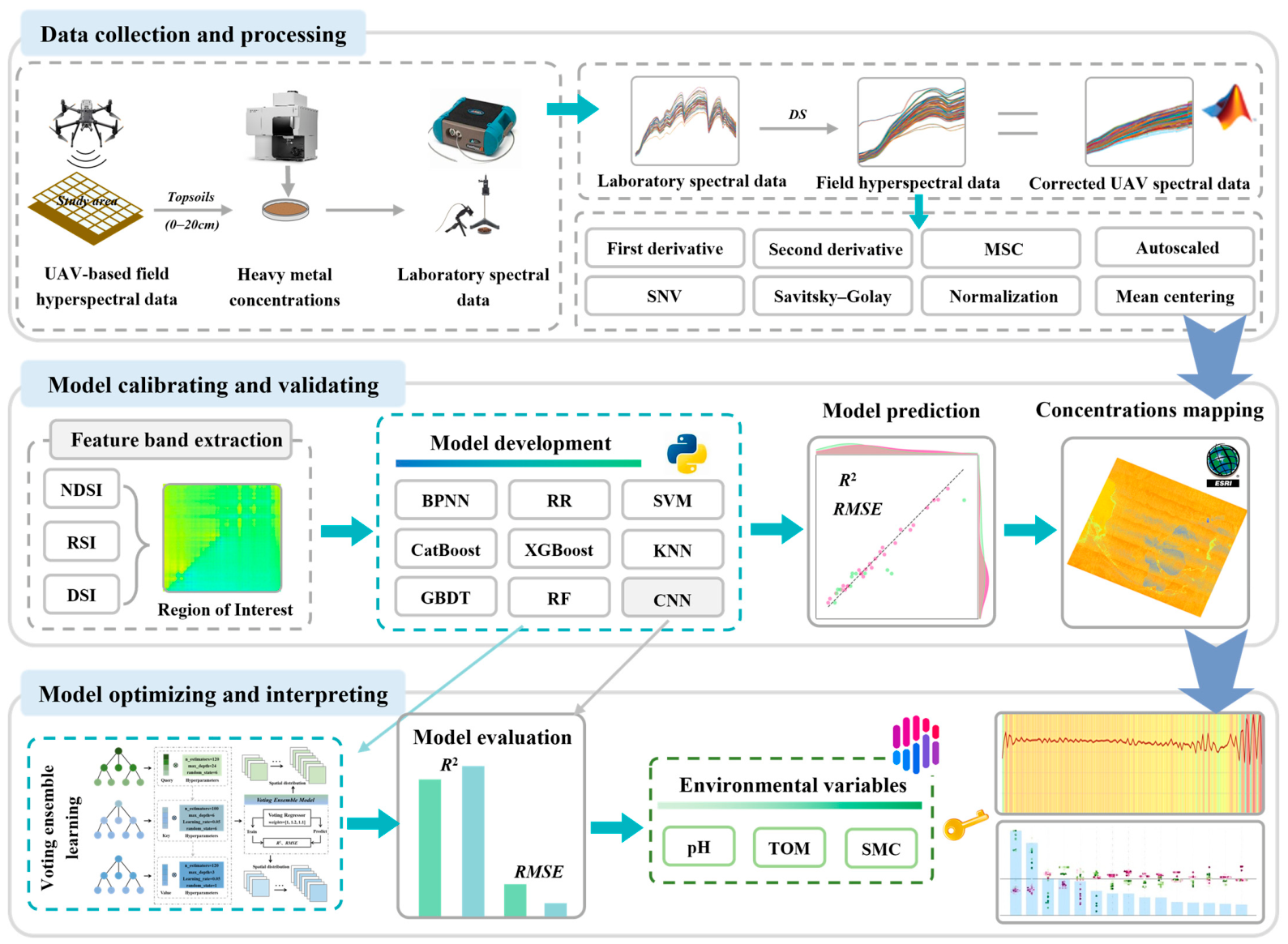
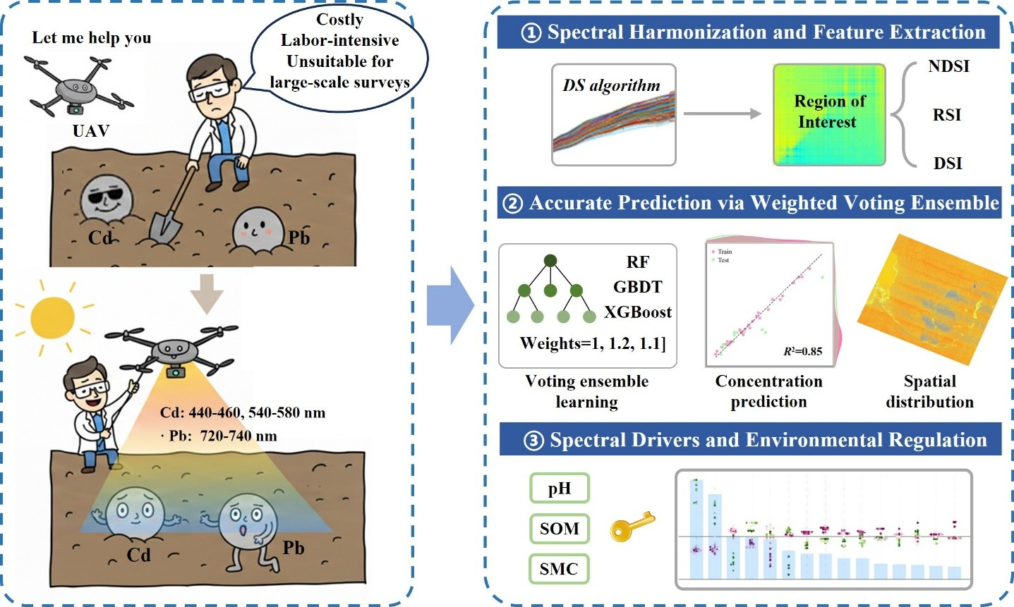
The overall methodological framework of this study is illustrated in Figure 2 and proceeds through three integrated stages. The first stage, data acquisition and preprocessing, involved acquiring hyperspectral imagery of surface soils using a UAV sensor, in coordination with ground sampling and field survey layouts. Soil samples were analyzed in the laboratory using an ASD FieldSpec3 portable spectroradiometer (Analytical Spectral Devices, Inc, Boulder, CO, USA) to obtain high-precision spectral curves, while heavy-metal concentrations were determined via ICP-AES. To mitigate spectral distortions caused by soil moisture, illumination variability, and other uncertain environmental factors, the DS algorithm was employed to calibrate the UAV field spectra against laboratory standards. Subsequently, eight preprocessing techniques were applied to the corrected spectra to generate a high-quality feature set for modeling.

The second stage, model construction and validation, focused on feature engineering and baseline algorithm benchmarking. After spectral standardization, multiple spectral indices—including DSI, RSI, and NDSI—were calculated to identify optimal wavelength combinations. Eight baseline machine learning models were then constructed using a unified training–testing split to ensure comparability. Model performance was rigorously evaluated using R² and RMSE, enabling the selection of the best-performing models for predicting heavy-metal concentrations and generating spatial distribution maps.

The third stage, model optimization and interpretation, advanced the framework by developing a voting ensemble model based on the integrated outputs of individual learners, which was systematically compared against a deep learning CNN model to assess stability across paradigms. To examine the influence of environmental conditions, soil pH, SOM, and SMC were incorporated as covariates to construct seven modeling scenarios. Based on these predictions, the SHAP method was employed to quantify feature contributions and interactions at both global and local scales, while Grad-CAM was applied to the CNN model to visualize convolutional activation patterns and reveal deep-level feature extraction mechanisms. This final phase aimed to identify sensitive spectral bands and response patterns, providing meaningful insights into pollution mechanisms and enhancing the physical interpretability of the inversion models.

3. Results and Discussion

3.1. Descriptive Statistics of the Heavy Metals Content

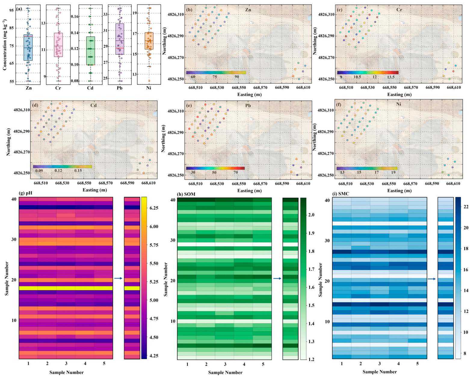
The descriptive statistics for in situ heavy-metal concentrations are visualized in Figure 3a. The mean concentrations of Zn, Cr, Cd, Pb, and Ni were 74.00, 11.29, 0.12, 29.73, and 16.29 mg·kg⁻¹, respectively. To further determine whether the measured concentrations differed significantly from the geochemical background values of Jilin Province, one-sample t-tests were performed for each metal. As shown in Figure 3a, the dark solid lines denote mean values and the red dashed lines represent the geochemical background of Jilin Province; distinct pollution patterns are evident. Cd was higher than the provincial background level, with an average concentration reaching 1.19 times the background value (t = 5.615, p < 0.001). Pb was slightly higher than its background value, with an average concentration reaching 1.03 times the provincial background level (t = 2.388, p = 0.0219). These statistical results indicate that Cd and Pb were the main elements showing enrichment relative to the local soil background. This accumulation is primarily attributed to the open-air storage of tailings, where fine-grained residues—characterized by large specific surface areas and abundant adsorption sites—act as effective carriers for these metals [46]. Furthermore, the absence of containment measures facilitates the mobilization of weakly bound and acid-soluble Cd and Pb via atmospheric deposition and rainfall leaching, resulting in localized hotspots [47,48]. In contrast, the mean concentrations of Zn, Cr, and Ni remained below their respective background thresholds and were significantly lower than the corresponding background values according to the one-sample t-tests (p < 0.001), suggesting no obvious enrichment relative to the provincial background (hence, no background reference lines are plotted for them).

The spatial distribution patterns of the five metals are depicted in Figure 3b–f, where color gradients indicate concentration levels and red contours highlight areas exceeding background limits. Spatially, elevated concentrations of Cd and Pb are not confined to the tailings deposition area (Area A) but extend significantly into Area B. This pattern suggests a source-to-sink migration pathway, where contaminants accumulated near the tailings have migrated downslope, forming a trans-regional dispersion plume [49,50]. Conversely, Zn, Cr, and Ni exhibit relatively stable spatial heterogeneity. Zn shows only sporadic high values associated with local mineral fragments, Cr displays a uniform distribution with minimal variance, and Ni presents a moderate gradient lacking distinct hotspots. These observations confirm that, unlike Cd and Pb, the distribution of Zn, Cr, and Ni is predominantly geogenic and less influenced by mining activities.

Additionally, the spatial characteristics of soil physicochemical properties—pH, SOM, and SMC—were analyzed across 200 within-site subsampling points (Figure 3g–i, left panels). These properties exhibited strong local spatial autocorrelation, evidenced by the high similarity in values among adjacent points within the same sampling site. To ensure consistency among laboratory heavy-metal measurements, UAV-extracted spectral features, and environmental covariates, and to reduce pseudo-replication caused by treating highly correlated within-site subsamples as independent observations, a spatial aggregation strategy was implemented. As shown in the “mean-value heatmaps” on the right side of Figure 3g–i, averaging the five subsamples within each predefined sampling site effectively preserved the underlying spatial structure while smoothing local fluctuations. This grouping approach ensures that the resulting 40 representative datasets retain the fundamental numerical and spatial characteristics of the original environmental field, providing robust input variables for subsequent modeling.

3.2. Characteristics of Soil Spectral Reflectance

3.2.1. Spectroscopic Calibration via Direct Standardization

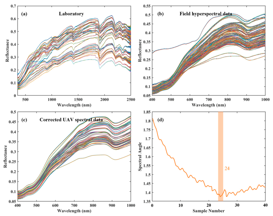
Field-acquired UAV spectra are inevitably affected by environmental factors such as fluctuating illumination, soil moisture heterogeneity, and atmospheric scattering. To recover high-fidelity surface reflectance, the direct standardization (DS) algorithm was applied to calibrate UAV imagery against high-precision laboratory ASD measurements. As shown in Figure A3 of Appendix A, laboratory spectra exhibited smooth and distinct curves with reflectance ranging from 0.10 to 0.55 and characteristic absorption features near 550, 1400, and 1900 nm (Appendix A Figure A3a), whereas the raw UAV spectra showed attenuated signals (reflectance ~0.05–0.40) and greater spectral fluctuations, particularly in the 700–900 nm region (Appendix A Figure A3b) reflecting the combined influence of field measurement conditions and soil-surface heterogeneity. After DS correction, the UAV spectra were better aligned with the laboratory reference spectra, with reflectance values increasing by approximately 5–15% in the visible–NIR range (450–900 nm), spectral fluctuations reduced, and diagnostic absorption features realigned with the laboratory reference spectra (Appendix A Figure A3c). To optimize the calibration model, the spectral angle mapper was used to determine the ideal transfer set size, and the mean spectral angle decreased sharply from 1.80 to 1.45 before stabilizing at approximately 24 samples; therefore, a transfer set of 24 samples was selected to construct the transformation matrix, ensuring the highest spectral similarity between corrected UAV data and laboratory spectra (Appendix A Figure A3d).

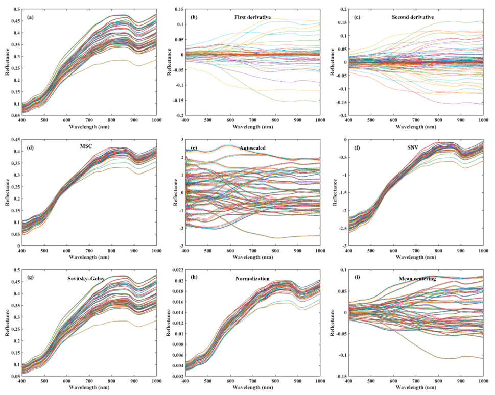
Based on the DS-corrected spectra, eight preprocessing techniques were further evaluated to enhance spectral discrimination and reduce residual noise that could affect feature extraction and model performance. Detailed results are presented in Appendix A.3, Figure A4b–i and

Table A4. Comparison of spectral preprocessing methods based on reflectance-curve characteristics.

Method	Curve Smoothness	Inter-Sample Dispersion	Shape Preservation	Main Effect	Selection
FD	High oscillation	Moderate	Low	Enhances local variation but amplifies noise	No
SD	Very high oscillation	Moderate	Low	Strongly enhances subtle features but amplifies high-frequency noise	No
MSC	Low	Low	High	Reduces scattering and improves curve consistency	Yes
Autoscale	Moderate	High	Moderate	Standardizes bands but may exaggerate local variation	No
SNV	Low	Low	High	Suppresses scattering noise and reduces dispersion	Yes
SG	Lowest	Moderate	High	Smooths spikes and high-frequency noise	Yes
Normalization	Low	Low	Moderate	Compresses dynamic range	No
Mean centering	Moderate	Moderate	Moderate	Enhances relative variation but retains noise	No

. Among these methods, MSC and SNV (Appendix A Figure A4d,f) effectively reduced scattering effects across the full spectral range and improved the consistency among spectral curves [51,52], while SG smoothing (Appendix A Figure A4g) substantially suppressed spectral spikes and high-frequency oscillations, producing smoother and more continuous reflectance profiles [53]. After comprehensive evaluation of spectral fluctuation reduction, feature enhancement, curve consistency, and preservation of original spectral information, the MSC-, SNV-, and SG-processed spectra were selected for subsequent feature band identification.

3.2.2. Spectral Preprocessing and Feature Band Selection

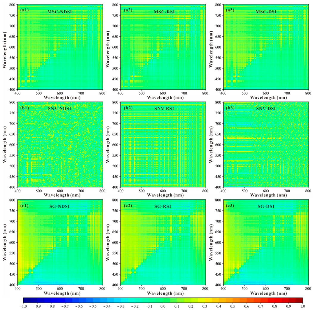
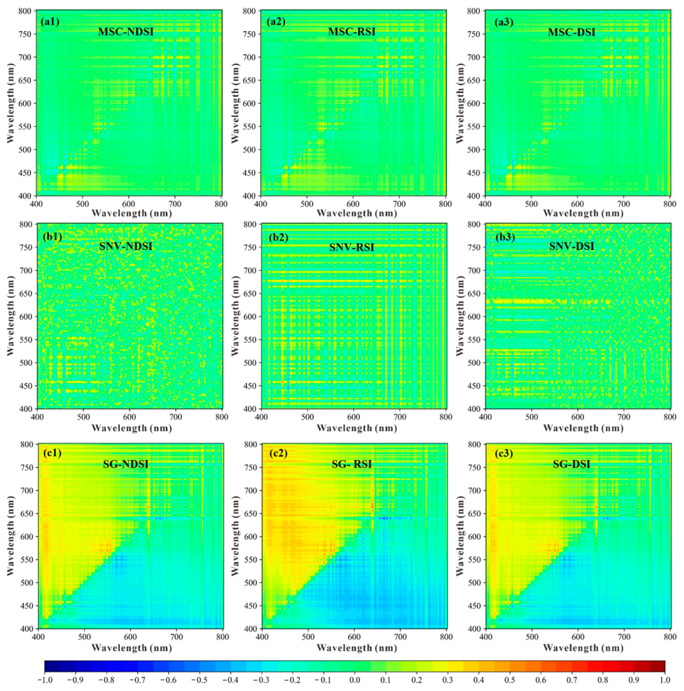
Using these three preprocessing methods, region of interest (ROI) correlation coefficient matrices was generated to extract characteristic bands related to Cd concentration for three spectral indices (NDSI, RSI, and DSI). The two-dimensional correlation patterns (Figure 4(a1–c3)) show that MSC and SNV preprocessing yield relatively uniform strip-like gradients, whereas SG preprocessing produces more distinct block-like clusters of high-correlation regions. Colors predominantly distributed within the blue–orange range indicate strong spectral responses associated with Cd. A threshold of |r| > 0.5 was applied for initial screening to extract band combinations exhibiting strong indicative capacity [54].

After preliminary screening, candidate band combinations were ranked based on correlation magnitude. Several combinations demonstrate strong associations with Cd concentration. Among them, SG-processed NDSI (449 nm, 457 nm), DSI (449 nm, 457 nm), and RSI (557 nm, 570 nm) exhibit the highest correlation coefficients (0.65, 0.63, and 0.61, respectively), all exceeding 0.6. These highly responsive bands are primarily located in the blue region (450–500 nm) and green region (550–600 nm), which correspond to key absorption features of iron oxides, organic matter, and clay minerals [55]. Reflectance variations within these regions are largely driven by changes in Fe³⁺ content, aluminosilicates, and soil organic matter—components closely linked to Cd adsorption and complexation processes [56]. Thus, these wavelengths serve as effective indirect indicators of Cd enrichment. Spatial consistency across preprocessing methods further validates the reliability of these bands. Considering correlation strength, spatial distribution, and the superior smoothing performance of SG filtering, the SG-derived high-correlation band combinations were selected as the final spectral features for Cd inversion modeling.

The same feature extraction workflow was applied to identify characteristic spectral bands associated with Pb concentration. The correlation coefficient matrices for Pb (Appendix A Figure A5(a1–c3)) reveal patterns distinct from those of Cd. Pb-sensitive high-correlation regions occur predominantly within the red to red-edge region (650–750 nm) and partly within the green region (580–620 nm). SG preprocessing again yields the most coherent and concentrated correlation clusters. Applying the |r| > 0.5 threshold and ranking candidate band pairs shows that Pb exhibits its strongest spectral response in the red-edge domain. Specifically, NDSI (640 nm, 665 nm), RSI (640 nm, 665 nm), and DSI (640 nm, 665 nm) achieve correlation coefficients of 0.72, 0.80, and 0.72, respectively—substantially higher than other band combinations. The red-edge region is highly sensitive to changes in soil biochemical and microstructural properties. Pb enrichment—via adsorption, accumulation, or surface complexation—modifies soil matrix components, thereby amplifying indirect spectral responses within this region [57]. Based on correlation magnitude, spatial coherence, and preprocessing stability, the SG-derived red-edge band combinations were selected as the optimal spectral features for Pb inversion modeling.

3.3. Model Performance Evaluation

3.3.1. Preliminary Performance Screening of Machine Learning Models

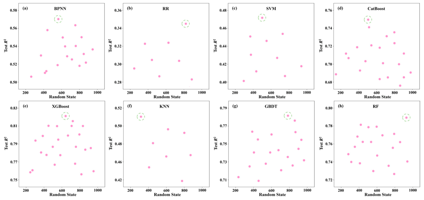
To systematically assess the suitability of different machine learning techniques for heavy-metal concentration inversion, eight models—BPNN, RR, SVM, CatBoost, XGBoost, KNN, GBDT, and RF—were constructed and evaluated. Given that random data partitioning can markedly affect model training outcomes and generalization ability, each model was trained using 1000 random seeds, and the corresponding test-set coefficients of determination (Test R²) were recorded to characterize the sensitivity of model performance to data splits. The repeated partitions were used to describe the overall stability of each model across different data splits, rather than to determine the final result from the single split with the highest Test R². Therefore, model performance was interpreted based on the distributional characteristics of Test R² across repeated partitions.

As illustrated in Figure A6 of Appendix A, substantial differences were observed among the models in both the number of valid random seeds and the associated prediction accuracy. The overall performance of BPNN (Appendix A Figure A6a), RR (Appendix A Figure A6b), SVM (Appendix A Figure A6c), and KNN (Appendix A Figure A6f) was relatively poor, with their maximum Test R² reaching only 0.57, 0.35, 0.47, and 0.51, respectively. The majority of Test R² values for these models clustered below 0.50, indicating strong dependence on data partitioning and limited generalization capability—insufficient to support reliable heavy-metal inversion [58].

In contrast, CatBoost (Appendix A Figure A6d), XGBoost (Appendix A Figure A6e), GBDT (Appendix A Figure A6g), and RF (Appendix A Figure A6h) demonstrated much higher predictive stability. Their upper-range Test R² values all exceeded 0.75, and a large proportion of random seeds resulted in Test R² values consistently distributed within the 0.70–0.80 range. This indicates that tree-based ensemble frameworks offer greater robustness to variations in data partitioning and superior predictive capability. Similar performance patterns were observed for Pb, reinforcing the conclusion that ensemble models provide more reliable inversion performance for both heavy metals. These four models were therefore selected as the most suitable candidates for subsequent prediction and inversion analyses.

3.3.2. Evaluation of Heavy-Metal Concentration Prediction

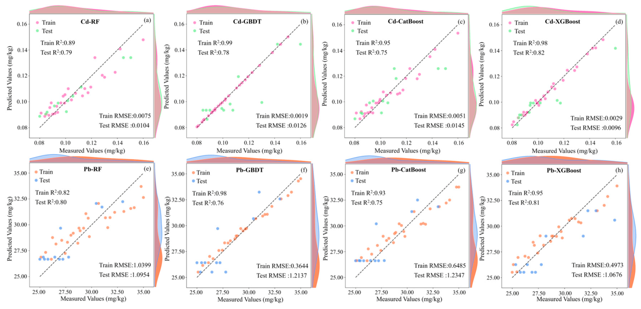
Using a fixed representative data split for visualization and model comparison, the predictive performance of the four best-performing algorithms—CatBoost, XGBoost, GBDT, and RF—was further assessed by comparing measured and predicted concentrations of Cd and Pb (Figure 5). For Cd (Figure 5a–d), XGBoost (Figure 5d) achieved the highest predictive accuracy, with a Test R² of 0.82 and prediction points tightly concentrated around the 1:1 line. CatBoost (Figure 5c) showed slightly inferior performance, with test points displaying broader dispersion. RF (Figure 5a) and GBDT (Figure 5b) produced comparable Test R² values of 0.78 and 0.79 but exhibited mild systematic deviations—especially in the low-concentration interval—suggesting remaining instability. All four models yielded very high training R² values (0.89–0.99), considerably higher than their test-set performance, indicating persistent overfitting despite optimization of random seeds [59].

For Pb (Figure 5e–h), despite a wider concentration range and more pronounced spectral heterogeneity, the models maintained strong predictive capability with Test R² values ranging from 0.75 to 0.81. RF (Figure 5e) and XGBoost (Figure 5h) again performed the best, underscoring the robustness of tree-based algorithms across different heavy metals and spectral conditions.

Although model performance improved significantly, two primary limitations remain: (1) Prediction accuracy remains capped. None of the models exceeded a Test R² of 0.85, which restricts their suitability for high-precision inversion applications. (2) Sensitivity to local data distributions persists. CatBoost exhibited notable deviations at both low and high concentrations, suggesting that existing models insufficiently capture the complex nonlinear relationships between spectral features and heavy-metal concentrations. To further enhance accuracy, mitigate overfitting, and better learn multiscale nonlinear spectral–concentration relationships, integrating ensemble strategies or adopting deep learning architectures is necessary.

3.3.3. Comparison of Ensemble and CNN Models and Mapping of Heavy-Metal Concentrations

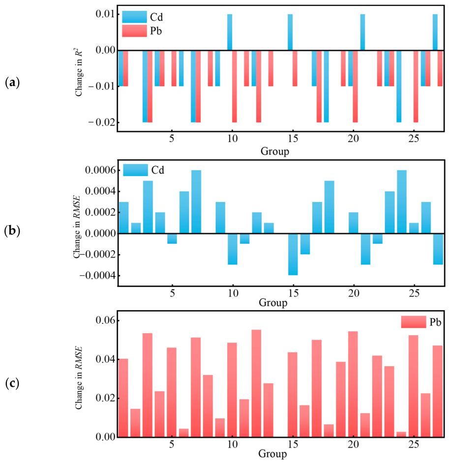
To improve prediction stability and reduce dependence on single-model performance, a voting ensemble model was built by integrating RF, GBDT, and XGBoost, leveraging their complementary strengths in feature interpretation, nonlinear learning, and decision boundary delineation [60,61]. Based on the performance variability observed during training and testing, differential weights (RF: 1.0, GBDT: 1.2, XGBoost: 1.1) were assigned, and a soft-voting strategy was implemented for weighted fusion. To further evaluate the sensitivity of the voting ensemble to weight settings, the baseline weights of RF, GBDT, and XGBoost were perturbed by ±20%, resulting in 27 weight combinations. The corresponding Test R² and RMSE values were then compared to evaluate the influence of ensemble-weight variation on model performance (Figure A7). In parallel, a CNN model was developed using spectral reflectance combinations as input, allowing the multi-layer convolutional architecture to extract hierarchical local–global joint features. This enabled a comparative evaluation of ensemble learning and deep learning in modeling heavy-metal spectral responses.

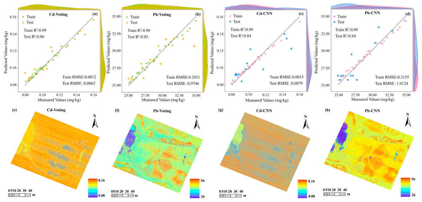
As shown in Figure 6a–d, both the voting and CNN models achieved considerable improvements over the base models. The voting model demonstrated stable R² values of 0.85–0.86, while the CNN model achieved 0.84. Although both surpassed the highest base-model accuracy (approximately 0.82), the difference between the voting and CNN models was small; therefore, the slightly higher R² of the voting model should be interpreted as a marginal numerical advantage. Prediction points for the voting model (Figure 6a,b) closely followed the 1:1 line across all concentration ranges, indicating relatively stable error control. In contrast, the CNN model, while maintaining strong overall fitting performance, showed greater dispersion in medium to high concentration intervals (Figure 6c,d). This suggests that under constraints of limited sample size and modest spectral dimensionality, the CNN model may be more sensitive to local concentration variability and data partitioning.

After model performance evaluation, both optimal models were used to generate spatially continuous Cd and Pb distribution maps (Figure 6e–h). The voting model produced smooth gradients and high spatial coherence (Figure 6e,f), making it suitable for interpreting large-scale pollution patterns. In contrast, CNN-generated maps (Figure 6g,h) displayed enhanced local texture features and stronger spatial heterogeneity. For example, CNN detected fine-scale variations in low-concentration Cd regions (Figure 6g), generating fragmented high-value patches. For Pb (Figure 6h), multiple discrete high-concentration hotspots were identified, which corresponded well with bare land, stockpiles, and areas of human disturbance. This demonstrates CNN’s heightened sensitivity to fine-grained surface features and its capacity to capture localized pollution anomalies [62].

In summary, the voting ensemble model showed a slight numerical advantage and relatively stable error distribution, benefiting from the complementary strengths of multiple learning mechanisms. Conversely, CNN excels at capturing subtle spatial variations, detecting hotspots, and characterizing local heterogeneity. Together, the two approaches offer a multi-scale inversion framework—from broad pollutant gradients to localized anomaly detection—supporting more comprehensive heavy-metal pollution assessment.

3.4. Spatial Analysis and Model Interpretation in Black Box Systems

3.4.1. Effects of Different Environmental Covariates on Model Accuracy

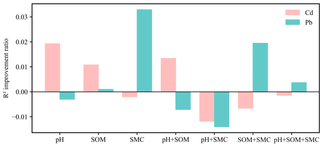
Since the voting model established in Section 3.3.3 achieved the best overall predictive performance among all tested models, it was used as the reference model for the subsequent environmental–covariate coupling analysis. Based on the multi-scenario input framework established in Section 2.5, this study systematically evaluated how pH, SOM, SMC, and their combinations influence model prediction accuracy, where pH, SOM, and SMC represent the mean values of the five subsamples within each sampling site. Figure 7 presents the R² improvement under different input scenarios relative to the voting baseline. Pink bars represent Cd and green bars represent Pb. Positive values indicate accuracy enhancement relative to the voting baseline, whereas negative values reflect performance degradation following the introduction of environmental variables.

For Cd, adding pH or SOM in single-variable scenarios resulted in notable accuracy gains, each increasing R² by more than 0.01. In contrast, SMC produced a slight negative effect, indicating that Cd’s spectral behavior is more strongly associated with soil acidity/alkalinity and organic matter, whereas its dependence on moisture is comparatively weak. In multi-factor scenarios, the combination of pH + SOM continued to provide meaningful improvements (R² increase ≈ 0.02). However, both pH + SMC and SOM + SMC yielded performance declines, with pH + SMC showing the strongest negative impact (R² reduction > 0.01). This suggests that moisture input weakens the beneficial regulatory effects of pH or SOM, implying a compensatory interaction among covariates [63]. The three-factor combination (pH + SOM + SMC) did not produce synergistic enhancement. Instead, it slightly decreased prediction accuracy, indicating that simultaneous integration of all variables introduces complex inter-variable interference rather than complementary information.

For Pb, the single-variable patterns differed substantially from those of Cd. The addition of pH produced a negative effect (R² decrease ≈ 0.01), suggesting that Pb’s spectral–concentration relationship does not benefit from pH variation and that pH may introduce additional noise. SOM contributed only a marginal improvement (<0.01). By contrast, SMC yielded the largest positive effect among all single variables, increasing R² by more than 0.03. This highlights the central role of soil moisture in influencing Pb mobility, solubility partitioning, and pore-water redistribution in soils [64]. In multi-factor scenarios, pH + SOM and pH + SMC produced negative effects, with pH + SMC again showing strong attenuation (>0.01), indicating that pH disrupts the strong positive influence of moisture. Conversely, SOM + SMC generated the greatest positive gain (R² increase > 0.02), suggesting that Pb exhibits clearer adsorption–desorption behavior under coupled moisture–organic matter conditions. These complementary interactions enhance the model’s ability to capture Pb fixation and migration processes. Although the three-factor combination (pH + SOM + SMC) also improved prediction accuracy, the magnitude was lower than that of SOM + SMC alone, indicating that pH does not provide additional useful information for Pb and may weaken the stable synergy already formed between SOM and SMC.

Overall, the environmental covariate effects reflect a pattern of “dominant single-factor influence with partial attenuation in multi-factor conditions.” Cd prediction is strongly regulated by pH and SOM, whereas Pb prediction is most sensitive to moisture, forming two distinct environmental response modes. Furthermore, the findings demonstrate that adding more covariates does not necessarily improve performance; in some cases, multi-factor combinations introduce redundant or conflicting information, reducing accuracy and underscoring the complex nonlinear interactions among soil physicochemical attributes in spectral inversion modeling.

3.4.2. Screening of Characteristic Variables Based on SHAP

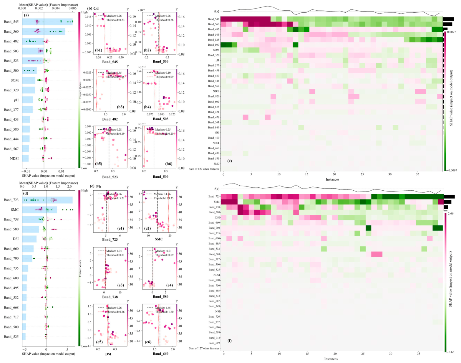
SHAP analysis was applied to spectral bands, environmental covariates, and spectral indices to identify model-derived feature contributions and potential associations underlying the voting model’s predictions. The analysis was conducted at three levels: global feature contribution (Figure 8a,d), feature response patterns (Figure 8b,e), and feature–feature interaction structures (Figure 8c,f). It should be noted that SHAP values provide model-based interpretability rather than direct evidence of causality; therefore, the following interpretations should be regarded as potential associations between input variables and model predictions.

Global SHAP bar plots (Figure 8a,d) summarize the top 15 contributing variables for Cd and Pb. Mean absolute SHAP values quantify each feature’s overall influence on model output, bar length indicates relative importance, and the colored scatter points reflect the direction and distribution of contributions across samples. For Cd (Figure 8a), spectral variables constituted the majority of key contributors. Eleven of the top fifteen features were spectral bands, with Band_545, Band_560, Band_482, and Band_503 ranking among the most influential. These wavelengths fall within the blue–green region (450–650 nm), which may be associated with organic matter and clay mineral absorption features related to Cd variation. Among local environmental factors, SOM and pH contributed substantially more than SMC, aligning with Section 3.4.1, and suggesting that acidity–organic matter conditions may provide useful auxiliary information for Cd prediction. Overall, Cd prediction followed a “spectra-dominated with pH/SOM enhancement” contribution pattern.

For Pb (Figure 8d), the feature importance structure differed markedly. SMC was the only environmental variable among the top contributors, yet its SHAP magnitude surpassed most visible–near-infrared bands, consistent with its strong model contribution observed in Section 3.4.1. Spectrally, Pb showed higher SHAP magnitudes than Cd but with a more dispersed pattern. Sensitive wavelengths for Pb were mainly concentrated in the red-edge range (650–750 nm), such as Band_723 and Band_738. These bands displayed strong but mixed positive–negative contributions across samples, suggesting greater sensitivity of Pb prediction to micro-environmental variability and potentially contributing to the relatively lower Pb prediction accuracy compared with Cd.

Dependence plots (Figure 8b,e) highlight typical model response patterns. For Cd, key bands such as Band_545 and Band_560 exhibited smooth monotonic relationships: higher reflectance generally corresponded to stronger positive SHAP contributions. SOM and pH likewise showed relatively stable, monotonic trends. In contrast, Pb responses were more irregular. For SMC, SHAP values frequently switched direction within the same magnitude range, exhibiting strong vertical dispersion. Key indices and red-edge bands such as Band_723 and Band_738 also displayed alternating positive–negative clusters, suggesting that Pb prediction may be more sensitive to localized environmental variability and less directionally stable than Cd prediction.

SHAP interaction heatmaps (Figure 8c,f) further illustrate differences in feature contribution structures across samples [65]. Cd exhibited relatively highly coherent patterns: core bands showed continuous gradients of increasing contribution from low to high concentrations, forming stable, directionally consistent blocks. This suggests that Cd prediction may be associated with more consistent spectral–environmental response patterns across the dataset. In contrast, Pb’s SHAP patterns were fragmented, with SMC and red-edge bands frequently oscillating between positive and negative contributions across adjacent samples. This suggests that Pb prediction may be more affected by micro-environmental heterogeneity, resulting in a weaker and less stable global response pattern.

3.4.3. Grad-CAM-Based Visualization of CNN Spectral Attention and Deep Feature Responses

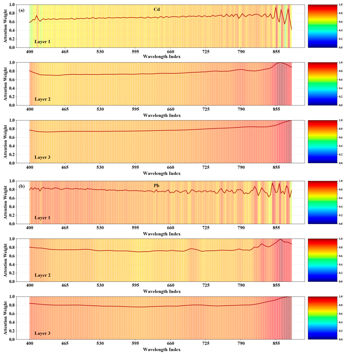
To further clarify the model-level spectral response patterns of the CNN model in heavy-metal inversion, Grad-CAM visualization was employed to analyze spectral attention distributions across convolutional layers [66]. Considering the relatively small site-level sample size, the Grad-CAM results were interpreted as qualitative evidence of CNN attention. Figure 9 shows the activation patterns for Cd and Pb across the 400–900 nm spectral range. For Cd (Figure 9a), the CNN consistently emphasized three key intervals: 440–480 nm, 540–580 nm, and 840–900 nm. This multi-segment activation pattern in the visible region, combined with near-infrared signal enhancement, suggests that the CNN integrate spectral information from multiple regions to support Cd prediction. For Pb (Figure 9b), the CNN exhibited a relatively focused attention structure. The strongest and most stable activation occurred within the 700–760 nm red-edge region and was observed across different convolutional layers. This indicates that Pb detection is primarily governed by small reflectance shifts and slope variations in the red-edge, which encode key information about Pb-induced modifications to soil microstructure. The 850–900 nm interval displayed only moderate auxiliary activation, suggesting that although the CNN incorporates structural cues from this region, the red-edge appeared to be an important spectral region in this dataset for Pb discrimination.

3.5. Identification of Heavy-Metal-Sensitive Wavelengths via Multi-Model Sensitivity Analysis

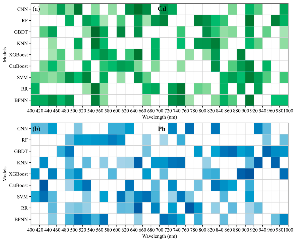
To further validate the physical interpretability of the inversion models, this section presents a comprehensive analysis of the key sensitive wavelengths identified by various models to pinpoint the primary spectral regions that respond to Cd and Pb concentrations. Figure 10 illustrates the sensitivity distributions of nine models across the 400–1000 nm wavelength range. The sensitive bands were determined based on both the frequency with which specific wavelengths were selected by the models and the intensity of their response (represented by color depth).

For Cd (Figure 10a), the models show pronounced sensitivity in the ranges of 440–460 nm, 540–580 nm, 820–860 nm, and 900–920 nm. Among these, the 540–580 nm region stands out as the most consistent and stable Cd-sensitive area across the models, with a continuous cluster of deep-colored blocks. This suggests that this band is a key spectral region for Cd prediction, particularly due to its strong association with the absorption features of organic matter and clay minerals in the blue–green region. These indirect spectral signals serve as significant indicators of Cd variation. For Pb (Figure 10b), the primary sensitive intervals are concentrated in 480–540 nm, 720–740 nm, and 900–920 nm. Notably, the 720–740 nm red-edge region exhibits a continuous deep-colored response across models, indicating its strongest sensitivity to Pb and the highest consistency among models. This finding reinforces the notion that the red-edge region is the most critical spectral area for capturing Pb-related variations [67]. Subtle reflectance transitions in this region, induced by Pb enrichment, allow models to extract more stable and pronounced Pb-related spectral features.

The key sensitive wavelengths for both Cd and Pb identified through multi-model sensitivity analysis show strong agreement with the characteristic bands derived from spectral index analysis in Section 3.2.2. This further validates the robustness of the proposed band-screening workflow. The combination of spectral-index-based prescreening and model sensitivity analysis proves to be an effective strategy for reliably extracting representative spectral features. This approach not only supports accurate inversion of soil heavy-metal concentrations but also lays a solid methodological foundation for subsequent feature reduction, model optimization, and cross-regional generalization. Beyond improving heavy-metal inversion accuracy, the established framework offers a scalable and transferable pathway for expanding spectral diagnostics to other heavy metals and critical soil physicochemical properties. This opens up substantial potential for advancing regional soil environmental monitoring, pollution risk assessment, and precision remediation strategies.

3.6. Limitations and Future Prospects

While this study provides valuable insights, several limitations remain that warrant further investigation. First, the spatial extent of the study area is relatively limited, with sampling sites concentrated in regions with higher levels of contamination. This may introduce spatial bias in the predictions, limiting the generalizability of the model. In addition, all soil samples and UAV hyperspectral images were collected during a single sampling period in April 2025, which limits the ability of the current dataset to capture seasonal variations in soil moisture, vegetation cover, illumination conditions, and heavy-metal mobility. Future research should expand sampling efforts to cover areas with varying pollution intensities and surface conditions and include multi-temporal observations across different seasons to enhance the model’s robustness and applicability. Meanwhile, in terms of model comparison, this study mainly evaluated representative machine learning, ensemble learning, and CNN models, while more recent advanced architectures were not included. Future studies should further compare the proposed framework with newer models using larger datasets to more comprehensively assess its relative performance. Future integration of three-dimensional hyperspectral LiDAR techniques may enable more precise characterization of surface structure and spectral information, thereby further improving the accuracy of soil heavy-metal estimation [68].

4. Conclusions

This study developed a rapid and interpretable UAV–laboratory synergistic framework for fine-scale mapping of soil heavy metals in mining environments. By applying the DS algorithm, field-induced spectral interference was effectively reduced, enabling reliable harmonization between UAV-acquired spectra and laboratory references. The weighted voting ensemble (RF–GBDT–XGBoost) achieved the best predictive performance (R² = 0.85), outperforming the individual single models and showing slightly higher stability than the CNN (R² = 0.84). While the ensemble model was more suitable for robust regional estimation, the CNN showed advantages in identifying localized hotspots, indicating complementary strengths for different monitoring purposes. Multi-scenario analysis and explainable AI (SHAP and Grad-CAM) further revealed distinct spectral–environmental associations in HMs prediction. Cd was mainly associated with blue–green bands (440–580 nm) and pH–SOM-related information, whereas Pb was dominated by red-edge bands (720–740 nm) and more strongly linked to SOM–SMC coupling. These results support the physical and geochemical consistency of the proposed framework. Overall, this study provides a site-specific UAV–laboratory synergistic approach for high-resolution HMs monitoring, mechanism-informed assessment, and targeted remediation in complex mining environments. Future work should further evaluate the framework across different soil types, mining settings and sampling seasons.

References

1. Yu, J.A.; Chen, Z.; Gao, W.H.; He, S.; Xiao, D.; Fan, W.; Huo, M.X.; Wahyunanto, A.N. Global trends and prospects in research on heavy metal pollution at contaminated sites. J. Environ. Manag. 2025, 383, 125402. [Google Scholar] [CrossRef]
2. Wei, Y.J.; Zheng, N.; An, Q.R.; Chen, C.C.; Pan, J.M.; Wang, S.; Peng, L.Y.; Qin, Y.F. Cr(VI) stress-driven enrichment of rhizosphere microbial functions and metabolic regulation synergistically reduce chromium bioavailability. J. Hazard. Mater. 2026, 501, 140786. [Google Scholar] [CrossRef]
3. Zhang, B.; Guo, B.; Zou, B.; Wei, W.; Lei, Y.Z.; Li, T.Q. Retrieving soil heavy metals concentrations based on GaoFen-5 hyperspectral satellite image at an opencast coal mine, Inner Mongolia, China. Environ. Pollut. 2022, 300, 118981. [Google Scholar] [CrossRef]
4. Li, Y.; Wang, S.; Gao, W.; He, L.; Xi, J.; Huo, Y.; Fan, W.; Lyu, T.; Huo, M. In-situ triboelectric nanogenerator for energy self-cycling electrochemical systems in wastewater treatment. Water Res. 2025, 289, 124916. [Google Scholar] [CrossRef]
5. Yang, H.R.; Huang, K.; Zhang, K.; Weng, Q.; Zhang, H.; Wang, F. Predicting Heavy metal adsorption on soil with machine learning and mapping global distribution of soil adsorption capacities. Environ. Sci. Technol. 2021, 55, 14316–14328. [Google Scholar] [CrossRef] [PubMed]
6. Chen, C.; Wang, Y.C.; Zhang, Y.X.; Zhao, Z.K.; Feng, H. Remote Sensing Hyperspectral Image Super-Resolution via Multidomain Spatial Information and Multiscale Spectral Information Fusion. IEEE Trans. Geosci. Remote Sens. 2024, 62, 5515216. [Google Scholar] [CrossRef]
7. Bai, J.; Huang, H.G.; He, B.B.; Ma, L.F.; Gao, S.A.; Peng, S.F.; Yang, X.B.; Hao, Y.S.; Dong, Y.B.; Bi, K.Y.; et al. The first large-footprint hyperspectral LiDAR model to attempt to reveal forest chlorophyll distribution heterogeneity from vertically layered spectral perspective utilizing 3D radiative transfer modeling. Int. J. Appl. Earth Obs. Geoinf. 2026, 146, 105060. [Google Scholar] [CrossRef]
8. Zakeri, F.; Mariethoz, G. A review of geostatistical simulation models applied to satellite remote sensing: Methods and applications. Remote Sens. Environ. 2021, 259, 112381. [Google Scholar] [CrossRef]
9. Wang, D.; Cao, L.Q.; Du, Y.H.; Xiong, H.Y.; Ye, F.W.; Zhong, Y.F. Toward noise-resilient retrieval of land surface temperature and emissivity using airborne thermal infrared hyperspectral imagery. ISPRS J. Photogramm. 2026, 231, 532–551. [Google Scholar] [CrossRef]
10. Zhang, S.; Zhao, G. A harmonious satellite-unmanned aerial vehicle-ground measurement inversion method for monitoring salinity in coastal saline soil. Remote Sens. 2019, 11, 1700. [Google Scholar] [CrossRef]
11. Meng, X.T.; Bao, Y.L.; Liu, J.G.; Liu, H.J.; Zhang, X.L.; Zhang, Y.; Wang, P.; Tang, H.T.; Kong, F.C. Regional soil organic carbon prediction model based on a discrete wavelet analysis of hyperspectral satellite data. Int. J. Appl. Earth Obs. 2020, 89, 102111. [Google Scholar] [CrossRef]
12. Lu, J.S.; Qi, Q.M.; Zheng, G.J.; Eitel, J.U.H.; Zhang, Q.Y.; Zhang, J.Y.; Chen, S.M.; Zhang, F.; Fang, W.M.; Guan, Z.Y.; et al. High-Throughput Field Phenotyping Using Unmanned Aerial Vehicles (UAVs) for Rapid Estimation of Photosynthetic Traits. Plant Phenomics 2025, 7, 100045. [Google Scholar] [CrossRef]
13. Ji, W.; Rossel, R.A.V.; Shi, Z. Improved estimates of organic carbon using proximally sensed vis-NIR spectra corrected by piecewise direct standardization. Eur. J. Soil. Sci. 2015, 66, 670–678. [Google Scholar] [CrossRef]
14. Song, Q.; Gao, X.H.; Song, Y.T.; Li, L.Q.; Chen, Z.; Li, R.X.; Zhang, H.; Cai, S.J. Estimation and mapping of soil texture content based on unmanned aerial vehicle hyperspectral imaging. Sci. Rep. 2023, 13, 14097. [Google Scholar] [CrossRef]
15. Feng, Y.; Wang, J.L.; Tang, Y.L. Estimation and inversion of soil heavy metal arsenic (As) based on UAV hyperspectral platform. Microchem. J. 2024, 207, 112027. [Google Scholar] [CrossRef]
16. He, Y.F.; Cai, X.M.; Dong, S.H.; Wang, S.L.; Li, C.B.; He, F. Estimation of spatial distribution of heavy metals in soils of mining areas based on ensemble learning and multi-source environmental variables: Application of LGGWR model. J. Hazard. Mater. 2026, 501, 140684. [Google Scholar] [CrossRef]
17. Chen, Y.N.; Shi, W.Y.; Aihemaitijiang, G.; Zhang, F.; Zhang, J.Q.; Zhang, Y.C.; Pan, D.Q.; Li, J.Y. Hyperspectral inversion of heavy metal content in farmland soil under conservation tillage of black soils. Sci. Rep. 2025, 15, 354. [Google Scholar] [CrossRef]
18. Tan, K.; Wang, H.M.; Chen, L.H.; Du, Q.; Du, P.J.; Pan, C.C. Estimation of the spatial distribution of heavy metal in agricultural soils using airborne hyperspectral imaging and random forest. J. Hazard. Mater. 2020, 382, 120987. [Google Scholar] [CrossRef]
19. Shen, L.Z.; Gao, M.F.; Yan, J.W.; Li, Z.L.; Leng, P.; Yang, Q.; Duan, S.B. Hyperspectral Estimation of Soil Organic Matter Content using Different Spectral Preprocessing Techniques and PLSR Method. Remote Sens. 2020, 12, 1206. [Google Scholar] [CrossRef]
20. Sun, W.C.; Liu, S.; Zhang, X.; Li, Y. Estimation of soil organic matter content using selected spectral subset of hyperspectral data. Geoderma 2022, 409, 115653. [Google Scholar] [CrossRef]
21. Guo, X.C.; Qiu, Q.M.; Nettleton, D.; Schnable, P.S. High-Throughput Field Plant Phenotyping: A Self-Supervised Sequential CNN Method to Segment Overlapping Plants. Remote Sens. 2023, 5, 0052. [Google Scholar] [CrossRef]
22. Kakogeorgiou, I.; Karantzalos, K.G. HEvaluating explainable artificial intelligence methods for multi-label deep learning classification tasks in remote sensing. Int. J. Appl. Earth Obs. 2021, 103, 102520. [Google Scholar]
23. Gu, K.K.; Qi, H.D.; Li, G.N.; Wang, H.Q. Nonlinear impact of block spatial form on carbon pollution synergies in mining cities—An integrated analysis based on GWRF and SHAP. Sustain. Cities Soc. 2026, 136, 107057. [Google Scholar] [CrossRef]
24. Gan, W.X.; Zhang, Y.X.; Xu, J.Y.; Yang, R.Q.; Xiao, A.N.; Hu, X.D. Spatial Distribution of Soil Heavy Metal Concentrations in Road-Neighboring s Using UAV-Based Hyperspectral Remote Sensing and GIS Technology. Sustainability 2023, 15, 10043. [Google Scholar] [CrossRef]
25. Chen, Z.; Wang, S.; Xu, J.; He, L.; Liu, Q.; Wang, Y. Assessment and machine learning prediction of heavy metals fate in mining farmland assisted by Positive Matrix Factorization. J. Environ. Manag. 2024, 350, 119587. [Google Scholar] [CrossRef] [PubMed]
26. Zhou, X.T.; Liu, C.; Xue, Y.; Akbar, A.; Jia, S.J.; Zhou, Y.; Zeng, D.D. Radiometric calibration of a large-array commodity CMOS multispectral camera for UAV-borne remote sensing. Int. J. Appl. Earth Obs. 2022, 112, 102968. [Google Scholar] [CrossRef]
27. Tan, K.; Niu, C.; Jia, X.P.; Ou, D.P.; Chen, Y.; Lei, S.G. Complete and accurate data correction for seamless mosaicking of airborne hyperspectral images: A case study at a mining site in Inner Mongolia, China. ISPRS J. Photogramm. Remote Sens. 2020, 165, 1–15. [Google Scholar] [CrossRef]
28. Gholizadeh, A.; Saberioon, M.; Eyal, B.D.; Rossel, R.A.V.; Boruvka, L. Modelling potentially toxic elements in forest soils with viseNIR spectra and learning algorithms. Environ. Pollut. 2020, 267, 115574. [Google Scholar] [CrossRef] [PubMed]
29. Hong, Y.S.; Yu, L.; Chen, Y.Y.; Liu, Y.F.; Liu, Y.; Cheng, H. Prediction of Soil Organic Matter by VIS–NIR Spectroscopy Using Normalized Soil Moisture Index as a Proxy of Soil Moisture. Remote Sens. 2018, 10, 28. [Google Scholar] [CrossRef]
30. Ma, X.M.; Wang, J.L.; Zhou, K.F.; Zhang, W.Q.; Chen, A.P. Uncertainty in soil elemental prediction using machine learning and hyperspectral remote sensing. J. Hazard. Mater. 2025, 494, 138502. [Google Scholar] [CrossRef]
31. Ryu, J.H.; Oh, D.; Cho, J. Simple method for extracting the seasonal signals of photochemical reflectance index and normalized difference vegetation index measured using a spectral reflectance sensor. J. Integr. Agric. 2021, 20, 1969–1986. [Google Scholar] [CrossRef]
32. Shi, T.R.; Zhang, J.R.; Shen, W.J.; Wang, J.; Li, X.Y. Machine learning can identify the sources of heavy metals in agricultural soil: A case study in northern Guangdong Province, China. Ecotoxicol. Environ. Saf. 2022, 245, 114107. [Google Scholar] [CrossRef]
33. Asteris, P.G.; Nguyen, Q.H.; Vu, T.H.; Tran, L.T. Interpretable Machine Learning Model for Evaluating Flexural Strength of Ultra HighPerformance Concrete. Int. J. Transp. Sci. Technol. 2025, 6, 215–242. [Google Scholar] [CrossRef]
34. Zhang, W.Y.; Yang, D.Q.; Zhang, S. A new hybrid ensemble model with voting-based outlier detection and balanced sampling for credit scoring. Expert Syst. Appl. 2021, 174, 114744. [Google Scholar] [CrossRef]
35. Choi, J.; Lim, K.J.; Ji, B.J. Robust imputation method with context-aware voting ensemble model for management of water-quality data. Water Res. 2023, 243, 120369. [Google Scholar] [CrossRef]
36. Haruna, Y.; Qin, S.Y.; Chukkol, A.H.A.; Yusuf, A.A.; Bello, I.; Lawan, A. Exploring the synergies of hybrid convolutional neural network and Vision Transformer architectures for computer vision: A survey. Eng. Appl. Artif. Intell. 2025, 144, 110057. [Google Scholar] [CrossRef]
37. Zhao, X.; Zhao, D.; Wang, J.; Triantafilis, J. Soil organic carbon (SOC) prediction in Australian sugarcane fields using Vis–NIR spectroscopy with different model setting approaches. Geoderma Reg. 2022, 30, e00566. [Google Scholar] [CrossRef]
38. Liao, Y.; Dong, L.B.; Li, A.; Lv, W.W.; Wu, J.Z.; Zhang, H.L.; Bai, R.H.; Liu, Y.L.; Li, J.W.; Shangguan, Z.P.; et al. Soil physicochemical properties and crusts regulate the soil infiltration capacity after land-use conversions from farmlands in semiarid areas. J. Hydrol. 2023, 626, 130283. [Google Scholar] [CrossRef]
39. Wang, S.; Zhou, Y.; You, X.; Wang, B.; Du, L. Quantification of the antagonistic and synergistic effects of Pb2+, Cu2+, and Zn2+ bioaccumulation by living Bacillus subtilis biomass using XGBoost and SHAP. J. Hazard. Mater. 2023, 446, 130635. [Google Scholar] [CrossRef]
40. Brentan, B.M.; Menapace, A.; Oberascher, M.; Herrera, M.; Sitzenfrei, R. Enhancing explainable AI with graph signal processing: Applications in water distribution systems. Water Res. 2025, 285, 124022. [Google Scholar] [CrossRef] [PubMed]
41. Szandała, T. Unlocking the black box of CNNs: Visualising the decision-making process with PRISM. Inform. Sci. 2023, 642, 119162. [Google Scholar] [CrossRef]
42. Togawa, S.; Jin, K. Examination of the Relationship between Feature Extraction by Kernels and CNN Performance. In Proceedings of the IEEE International Symposium on Circuits and Systems (ISCAS), Singapore, 19–22 May 2024; pp. 1–5. [Google Scholar]
43. Xiang, X.; Guo, S.L.; Cui, Z.; Wang, L.; Xu, C.Y. Improving flood forecast accuracy based on explainable convolutional neural network by Grad-CAM method. J. Hydrol. 2024, 642, 131867. [Google Scholar] [CrossRef]
44. Selvaraju, R.R.; Cogswell, M.; Das, A.; Vedantam, R.; Parikh, D.; Batra, D. Grad-CAM: Visual Explanations from Deep Networks via Gradient-Based Localization. In Proceedings of the 2017 IEEE International Conference on Computer Vision (ICCV); IEEE: New York, NY, USA, 2017. [Google Scholar]
45. Mao, Y.C.; Liu, J.; Cao, W.; Ding, R.B.; Fu, Y.H.; Zhao, Z.G. Research on the quantitative inversion model of heavy metals in soda saline land based on visible-near-infrared spectroscopy. Infrared Phys. Technol. 2021, 112, 103602. [Google Scholar] [CrossRef]
46. Ge, J.; Wang, H.X.; Lin, J.Y.; Tian, S.K.; Zhao, J.Q.; Lin, X.Y.; Lu, L.L. Nickel tolerance, translocation and accumulation in a Cd/Zn co-hyperaccumulator plant Sedum alfredii. J. Hazard. Mater. 2020, 398, 123074. [Google Scholar] [CrossRef]
47. Su, C.X.; Rana, N.M.; Evans, S.G.; Wang, B.J.; Zhang, S.A. Tailings storage facilities in China: Historical failure incidents, existing status, and database-driven quantitative risk assessment. Int. J. Disaster Risk Reduct. 2024, 114, 104973. [Google Scholar] [CrossRef]
48. Fan, T.T.; Li, C.B.; Gao, J.; Zhou, D.M.; Alves, M.E.; Wang, Y.J. Wien effect of Cd/Zn on soil clay fraction and their interaction. Geochem. Trans. 2018, 19, 5. [Google Scholar] [CrossRef]
49. Geng, Y.C.; Wang, J.L.; Zhou, P.P.; Zhao, B.J.; Chen, Q.Y.; Qin, H.J.; Wang, Z.C.; Li, D.H. Vertical migration and transformation of metal(loid)s in surface layers of tailings ponds driven by induced biocrusts: Emphasizing arsenic and zinc dynamics. J. Hazard. Mater. 2025, 499, 140100. [Google Scholar] [CrossRef] [PubMed]
50. Luo, M.F.; Zhang, H.; Guo, J.h.; Zhao, J.; Feng, C.; Yin, J.L.; Xu, C.; Du, Y.; Liu, Y.; Lai, B. Proton vs. Electron: The Dual Role of Redox-Inactive Metal Ions in Permanganate Oxidation Kinetics. Environ. Sci. Technol. 2024, 40, 18041–18051. [Google Scholar] [CrossRef] [PubMed]
51. Han, C.; Lu, J.; Chen, S.; Xu, X.; Wang, Z.; Pei, Z.; Zhang, Y.; Li, F. Estimation of heavy metal(loid) contents in agricultural soil of the Suzi River Basin using optimal spectral indices. Sustainability 2021, 13, 12088. [Google Scholar] [CrossRef]
52. Zhang, S.; Shen, Q.; Nie, C.; Huang, Y.; Wang, J.; Hu, Q.; Ding, X.; Zhou, Y.; Chen, Y. Hyperspectral inversion of heavy metal content in reclaimed soil from a mining wasteland based on different spectral transformation and modeling methods. Spectrochim. Acta Pt. A-Mol. Biomol. Spectrosc. 2019, 211, 393–400. [Google Scholar] [CrossRef]
53. Cheng, H.; Shen, R.; Chen, Y.; Wan, Q.; Shi, T.; Wang, J.; Wan, Y.; Hong, Y.; Li, X. Estimating heavy metal concentrations in suburban soils with reflectance spectroscopy. Geoderma 2019, 336, 59–67. [Google Scholar] [CrossRef]
54. Che, S.A.; Du, G.Y.; Zhong, X.F.; Mo, Z.L.; Wang, Z.D.; Mao, Y.X. Quantification of Photosynthetic Pigments in Neopyropia yezoensis Using Hyperspectral Imagery. Plant Phenomics 2023, 5, 0012. [Google Scholar] [CrossRef] [PubMed]
55. Hong, Y.; Chen, S.; Liu, Y.; Zhang, Y.; Yu, L.; Chen, Y.; Liu, Y. Combination of fractional order derivative and memory-based learning algorithm to improve the estimation accuracy of soil organic matter by visible and near-infrared spectroscopy. Catena 2019, 174, 104–116. [Google Scholar] [CrossRef]
56. Terra, F.S.; Viscarra, R.A.; Demattê, J.A.M. Spectral fusion by Outer Product Analysis (OPA) to improve predictions of soil organic C. Geoderma 2019, 335, 35–46. [Google Scholar] [CrossRef]
57. Liu, X.; Ju, Y.W.; Mandzhieva, S.; Pinskii, D.; Minkina, T.; Rajput, V.D.; Roane, T.; Huang, S.Q.; Li, Y.P.; Ma, L.Q.; et al. Sporadic Pb accumulation by plants: Influence of soil biogeochemistry, microbial community and physiological mechanisms. J. Hazard. Mater. 2023, 444, 130391. [Google Scholar] [CrossRef]
58. MacKinnon, J.G.; Nielsen, M.; Webb, M.D. Testing for the appropriate level of clustering in linear regression models. J. Econom. 2023, 235, 2027–2056. [Google Scholar] [CrossRef]
59. Luan, J.; Zhang, C.L.; Xu, B.D.; Xue, Y.; Ren, Y.P. The predictive performances of random forest models with limited sample size and different species traits. Fish. Res. 2020, 227, 105534. [Google Scholar] [CrossRef]
60. Hong, Y.; Chen, Y.; Shen, R.; Chen, S.; Xu, G.; Cheng, H.; Guo, L.; Wei, Z.; Yang, J.; Liu, Y.; et al. Diagnosis of cadmium contamination in urban and suburban soils using visible-to-near-infrared spectroscopy. Environ. Pollut. 2021, 291, 118128. [Google Scholar] [CrossRef]
61. Sun, Y.; Chen, S.; Dai, S.; Li, D.; Jiang, H.; Jia, K. Coupled retrieval of heavy metal nickel concentration in agricultural soil from spaceborne hyperspectral imagery. J. Hazard. Mater. 2023, 446, 130722. [Google Scholar] [CrossRef]
62. Xie, Q.; Zhou, D.; Tang, R.; Feng, H. A Deep CNN-Based Detection Method for Multi-Scale Fine-Grained Objects in Remote Sensing Images. IEEE Access 2024, 12, 15622–15630. [Google Scholar] [CrossRef]
63. Khosravi, V.; Ardejani, F.D.; Yousefi, S.; Aryafar, A. Monitoring soil lead and zinc contents via combination of spectroscopy with extreme learning machine and other data mining methods. Geoderma 2018, 318, 29–41. [Google Scholar] [CrossRef]
64. Wekumbura, C.; Hettiarachchi, G.M.; Hargrove, W.; Ma, Q.; Newville, M.; Lanzirotti, A.; Sobin, C. Mitigating lead bioaccessibility in metal(loid)s contaminated alkaline soils using soil amendments: Evaluating efficacy using in vitro bioaccessibility, sequential extraction, and synchrotron techniques. J. Hazard. Mater. 2025, 497, 139742. [Google Scholar] [CrossRef]
65. Zhang, C.; Zhu, J.Y.; Mai, W.J.; Chen, Z.G.; Xie, Y.; Fu, S.; Xia, D.; Cai, C.; Zheng, W.B.; Liu, J.X.; et al. Satellite Remote Sensing-Implemented Nontargeted Screening of Emerging Contaminant Fingerprints in a River-to-Ocean Continuum through Interpretable Machine Learning: The Pivotal Intermediary Role of Dissolved Organic Matter. Environ. Sci. Technol. 2025, 59, 8714–8726. [Google Scholar] [CrossRef]
66. Shi, G.Y.; Wu, H.P.; Luo, S.H.; Lu, X.Y.; Ren, B.; Zhang, Q.; Lin, W.Q.; Chen, R.Y.; Guo, P.; Chen, H.B.; et al. 1D Gradient-Weighted Class Activation Mapping, Visualizing Decision Process of Convolutional Neural Network-Based Models in Spectroscopy Analysis. Environ. Sci. Technol. 2023, 95, 9959–9966. [Google Scholar] [CrossRef]
67. Yu, K.; Geel, M.V.; Ceulemans, T.; Geerts, W.; Ramos, M.M.; Serafim, C.; Sousa, N.; Castro, P.M.L.; Kastendeuch, P.; Najjar, G.; et al. Vegetation reflectance spectroscopy for biomonitoring of heavy metal. Environ. Pollut. 2018, 243, 1912–1922. [Google Scholar] [CrossRef]
68. Bai, J.; Niu, Z.; Wang, L. A theoretical demonstration on the independence of distance and incidence angle effects for small-footprint hyperspectral LiDAR: Basic physical concepts. Remote Sens. Environ. 2024, 315, 114452. [Google Scholar] [CrossRef]
Figure 1. Location and field conditions of the study area. (a) The study area in Yitong County, Jilin Province, Northeast China. (b) UAV orthophoto of the exposed open-pit tailings site and delineated sampling sub- areas A and B. (c) Field photographs of the two sampling sub-areas and systematic sampling layout used for investigating the spatial distribution of heavy-metal contamination.
Remotesensing 18 01687 g001
Figure 2. Workflow of the UAV–laboratory integrated hyperspectral inversion framework for soil heavy-metal prediction. The overall workflow consists of three major stages: (1) Data collection and processing, (2) Model calibrating and validating, and (3) Model optimizing and interpreting.
Remotesensing 18 01687 g002
Figure 3. Spatial distribution and descriptive statistics of heavy metals and soil physicochemical properties in the study area. (a) Boxplots showing the statistical characteristics of Zn, Cr, Cd, Pb, and Ni, where the deep-colored solid lines indicate the mean values and the red horizontal lines (where present) represent the geochemical background values of Jilin Province. (bf) Spatial distribution maps of each heavy metal, in which the color of each scatter point reflects its concentration and the red curves highlight sampling locations with values exceeding the provincial background levels. (gi) Heatmaps of the original 200 soil samples and the aggregated 40-sample averages for pH, SOM, and SMC.
Remotesensing 18 01687 g003
Figure 4. Two-dimensional correlation coefficient matrices between Cd concentration and spectral indices under different preprocessing methods. (a1a3) MSC-preprocessed spectra combined with NDSI, RSI, and DSI; (b1b3) SNV-preprocessed spectra combined with NDSI, RSI, and DSI; (c1c3) SG-preprocessed spectra combined with NDSI, RSI, and DSI.
Remotesensing 18 01687 g004
Figure 5. Comparison of the prediction performance of four machine learning models for Cd and Pb concentration estimation. (ad) Prediction scatterplots of RF, GBDT, CatBoost, and XGBoost for Cd, where pink points represent the training set and green points represent the testing set. (eh) Corresponding prediction scatterplots for Pb, with orange points denoting the training set and blue points denoting the testing set. The dashed line indicates the 1:1 reference line, and the marginal density curves illustrate the distribution patterns of measured and predicted values.
Remotesensing 18 01687 g005
Figure 6. Comparison of the prediction accuracy and spatial distribution results obtained by the voting and CNN models for Cd and Pb estimation. (a,b) Prediction scatterplots of the voting model for Cd and Pb, where green points represent the training set and orange points represent the testing set. (c,d) Prediction scatterplots of the CNN model for Cd and Pb, where pink points represent the training set and purple points represent the testing set. (e,f) Spatial distribution maps of Cd and Pb generated by the voting model. (g,h) Spatial distribution maps of Cd and Pb generated by the CNN model. The color bars denote concentration levels (mg/kg).
Remotesensing 18 01687 g006
Figure 7. Comparison of model performance improvements across different environmental covariate scenarios. R2 changes for Cd and Pb under seven input scenarios relative to the voting baseline, where pink bars represent Cd and green bars represent Pb.
Remotesensing 18 01687 g007
Figure 8. SHAP-based interpretation of the voting model for Cd and Pb prediction. (a,d) Global feature importance rankings showing the mean absolute SHAP values and contribution directions of spectral bands and environmental covariates. (b,e) Feature dependence plots, where (b1b6) and (e1e6) represent the top six contributing features for Cd and Pb, respectively, illustrating how SHAP values vary with feature magnitudes and indicating their response trends. (c,f) SHAP interaction heatmaps depicting the feature contribution structures and inter-feature interaction effects for Cd and Pb across samples.
Remotesensing 18 01687 g008
Figure 9. Grad-CAM-derived spectral attention distributions of the CNN for Cd (a) and Pb (b) across the 400–900 nm range. Each curve represents the normalized attention weights of a given convolutional layer, while the background colormap indicates the relative activation intensity (warmer colors denote stronger responses).
Remotesensing 18 01687 g009
Figure 10. Model-derived (CNN, RF, GBDT, KNN, XGBoost, CatBoost, SVM, RR, BPNN) sensitivity distributions of Cd (a) and Pb (b) across the 400–1000 nm spectral range. Each square represents the sensitivity intensity of a given model to a specific wavelength, where darker colors indicate stronger model responses.
Remotesensing 18 01687 g010
Disclaimer/Publisher’s Note: The statements, opinions and data contained in all publications are solely those of the individual author(s) and contributor(s) and not of MDPI and/or the editor(s). MDPI and/or the editor(s) disclaim responsibility for any injury to people or property resulting from any ideas, methods, instructions or products referred to in the content.