Adaptive Sliding-Window Filtering for GNSS SPP-Aided Orbit Determination in Earth–Moon Space

Highlights

What are the main findings?

• The proposed $C/N_0$-driven dynamic sliding-window strategy substantially improves GNSS SPP-aided orbit determination in Earth–Moon space over the conventional tightly coupled solution.
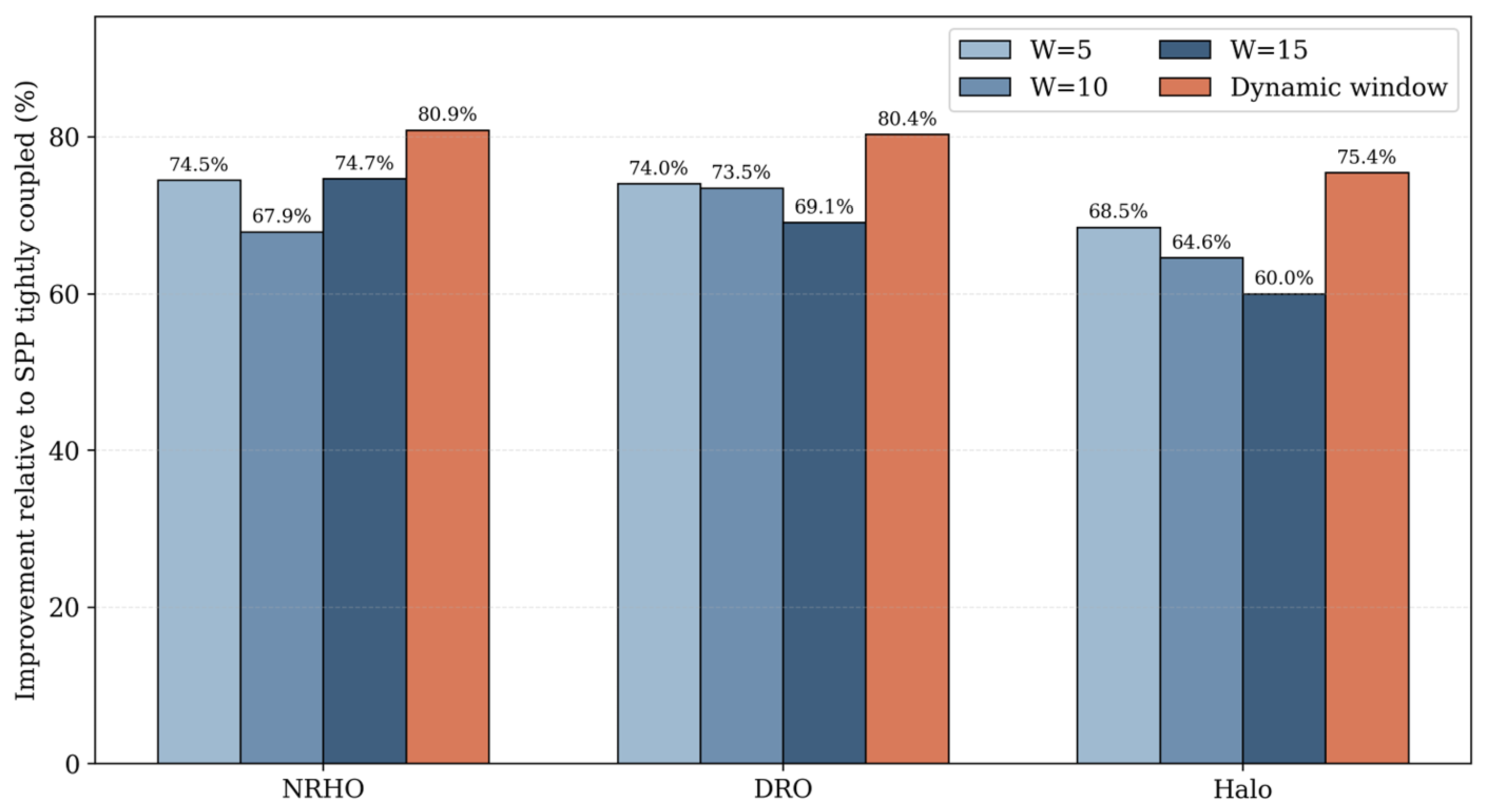
• For NRHO, DRO, and Halo trajectories, the method reduces the 3D RMS position error by 80.9%, 80.4%, and 75.4%, respectively, and provides the best overall balance among fixed- and dynamic-window schemes.

What are the implications of the main findings?

• Dynamic window regulation improves both long-arc stability and post-outage recovery, making adaptive covariance tuning a practical enhancement for autonomous cislunar navigation.
• The method is promising for future Earth–Moon missions operating under weak, intermittent, and time-varying GNSS observation conditions.

Abstract

Orbit determination in Earth–Moon space is challenged by dynamic-model mismatch and unstable GNSS observation conditions, especially under weak and intermittent signals. To address this issue, this paper proposes a GNSS single-point positioning (SPP)-aided orbit determination method based on adaptive sliding-window filtering. A tightly coupled framework is constructed by integrating orbital dynamics propagation with SPP pseudo-range observations, allowing propagation errors to be corrected in real time through measurement updates. To enhance adaptability under time-varying observation conditions, a dynamic sliding-window strategy is introduced, in which the observation-noise covariance is adjusted according to carrier-to-noise ratio ($C/N_0$) variations. Simulations for three representative Earth–Moon trajectories, including a near-rectilinear halo orbit (NRHO), a distant retrograde orbit (DRO), and a Halo orbit, show that the proposed method significantly outperforms the conventional tightly coupled solution. The three-dimensional RMS position error is reduced from 6.65 m to 1.27 m for NRHO, from 6.57 m to 1.27 m for DRO, and from 5.91 m to 1.44 m for Halo, corresponding to improvements of 80.9%, 80.4%, and 75.4%, respectively. Under a simulated 200-epoch GNSS interruption in the Halo case, the method also improves outage robustness and post-recovery performance, reducing the three-dimensional RMS error by 23.2% in the interruption-centered interval and by 26.1% over the full arc.

1. Introduction

With the sustained expansion of cislunar exploration and lunar mission planning, Earth–Moon space has become a key operational domain for transportation, science, and long-duration infrastructure deployment [1,2,3]. Representative mission concepts involving transfer trajectories, libration-point operations, and near-lunar orbits require spacecraft to maintain reliable orbit knowledge over long arcs and across rapidly changing dynamical regimes [1,4,5]. Under these conditions, real-time and autonomous orbit determination is increasingly important for navigation, guidance, and mission safety [6].

Dynamic orbit propagation remains the basic tool for spacecraft state prediction, but its long-arc accuracy in Earth–Moon space is limited by force-model mismatch, sensitivity to observational geometry, and phase-dependent nonlinear dynamics [5,7,8,9]. In practical cislunar applications, modeling errors associated with multi-body perturbations, orbit-maintenance dynamics, and numerical integration are gradually mapped into the propagated state and may lead to significant prediction drift if no external measurement correction is available [1,8,9]. Therefore, dynamic propagation alone is generally insufficient for robust autonomous orbit determination in Earth–Moon space.

Recent studies have shown that GNSS signals can still provide useful navigation information in cislunar and lunar environments, despite weak power levels and limited visibility compared with near-Earth operations [10,11,12]. At the same time, autonomous orbit-determination architectures for lunar and cislunar missions are being actively investigated using radio navigation, inter-satellite links, and multi-sensor fusion strategies [4,13,14]. These developments indicate that GNSS-assisted orbit determination is becoming a realistic option for future Earth–Moon missions, especially when onboard estimation must complement or partially replace continuous ground support.

A major challenge, however, is that the GNSS observation environment in Earth–Moon space is strongly time-varying. Weak signals, intermittent visibility, and changing geometric conditions can cause large fluctuations in measurement quality, making fixed-noise Kalman filtering difficult to maintain in both accuracy and consistency. To address similar issues, adaptive covariance-tuning and robust filtering strategies have been widely studied, including adaptive noise adjustment, adaptive cubature and extended Kalman filtering, smoothing-based covariance estimation, and classified adaptive factors [15,16,17,18,19,20,21,22,23,24]. In GNSS-related applications, Wang et al. developed an adaptive Kalman filter based on integer ambiguity validation for moving-base RTK [25], Jin et al. proposed an adaptive Kalman filtering framework based on an autoregressive predictive model [26], and Gao et al. applied a Helmert variance component estimation based adaptive Kalman filter in multi-GNSS PPP/INS tightly coupled integration [27]. In addition, fading-factor-based Kalman filtering has been applied in different GNSS-related navigation scenarios, including GPS/INS integrated navigation, GNSS pseudorange fault detection, and SINS/GNSS adaptive robust filtering, to enhance filter responsiveness under model mismatch, dynamic changes, or abnormal observations [28,29,30,31]. In parallel, $C/N_0$ has been shown to be an effective indicator for stochastic modeling in degraded GNSS environments [32,33,34], while sliding-window strategies provide a practical means for local statistical adaptation [35,36,37,38].

Despite these advances, most existing studies mainly focus on near-Earth GNSS positioning, integrated navigation, or general adaptive filtering problems, while the specific observation characteristics of Earth–Moon space have not been sufficiently considered. In cislunar scenarios, the received GNSS signals may come from the main-lobe edge or side-lobe regions, and their quality can vary rapidly with spacecraft–GNSS geometry and propagation distance. Therefore, a fixed observation-noise model or a fixed sliding-window length may be insufficient to balance responsiveness and robustness under such time-varying conditions.

To address this problem, this paper develops an adaptive sliding-window filtering method for GNSS SPP-aided orbit determination in Earth–Moon space. The method embeds SPP pseudo-range updates into a tightly coupled dynamic-estimation framework and uses the temporal variation in $C/N_0$ to regulate the effective window length for covariance adaptation. Sigmoid-based mapping is introduced to realize continuous window adjustment, so as to better balance responsiveness to abrupt observation-quality changes and robustness against short-term noise fluctuations. The main objective is to improve the adaptability of the tightly coupled filter under weak, intermittent, and time-varying GNSS observation conditions in Earth–Moon space. The remainder of this paper is organized as follows. Section 2.1 introduces the SPP-based tightly coupled model. Section 2.2 presents the adaptive sliding-window strategy and the dynamic window regulation mechanism. Section 3 reports the simulation setup and comparative results. Finally, Section 4 summarizes the conclusions and future work.

2. Materials and Methods

2.1. SPP-Based Tightly Coupled Dynamic Estimation Model

In conventional orbit determination, tightly coupled filtering combines dynamic orbit propagation with single-point positioning (SPP) observations to achieve continuous state estimation. The basic idea is to propagate the spacecraft state using the dynamic model and then use SPP pseudo-range observations to correct the predicted state, thereby suppressing the long-term divergence caused by cumulative propagation errors.

However, in Earth–Moon space, the observation quality may vary significantly due to weak signal strength, intermittent visibility, and changing observation geometry. To improve the robustness of the tightly coupled framework under such conditions, the proposed method incorporates an adaptive sliding-window strategy into the conventional filtering formulation. The detailed adaptive mechanism is presented in Section 3, while this section focuses on the state-space model used for dynamic propagation and SPP observation update.

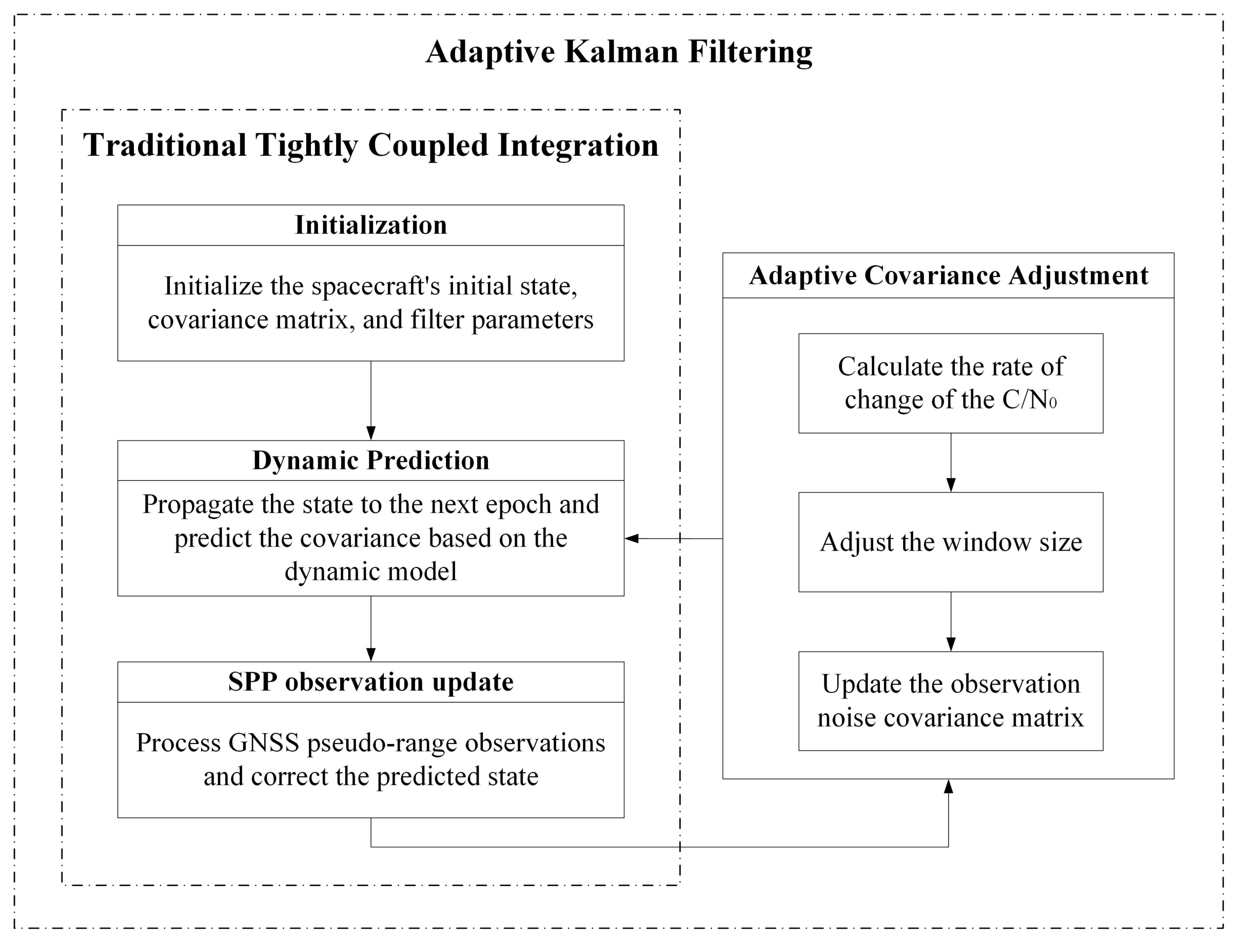
The overall framework consists of four steps: initialization, dynamic prediction, SPP observation update, and adaptive covariance adjustment. Figure 1 illustrates the overall tightly coupled adaptive filtering framework used in this study.

2.1.1. State Transition Model

In the tightly coupled framework, the spacecraft state is propagated by the orbital dynamic model and then corrected using SPP pseudo-range observations. Such measurement-aided state estimation has been widely adopted in integrated navigation and autonomous orbit-determination studies [11,39,40]. The continuous-time state model can be written as

$$\dot{X}(t)=F(X(t),t)+G(t)w(t)$$

(1)

where $X={\left[\begin{array}{cc}{r}^T& v^T\end{array}\right]}^T$ denotes the spacecraft state vector, including position $r$ and velocity $v$; $F(·)$ denotes the nonlinear orbital dynamic model; $G(t)$ is the process-noise distribution matrix; and $w(t)$ is the zero-mean Gaussian process noise. In this formulation, the filter state consists of the spacecraft position and velocity. The acceleration is not introduced as an independent state variable, because it is determined by the force model and is used only to propagate the position and velocity through the equations of motion. This is the standard state representation in dynamic orbit determination and avoids introducing additional weakly observable parameters under limited GNSS geometry.

For Earth–Moon orbit propagation, high-precision ephemeris support and accurate modeling of the Earth–Moon dynamical environment are required to represent the motion of the Moon and other perturbing bodies [1,8,41]. In this study, DE ephemerides are used, and the positions and velocities of celestial bodies are obtained by Chebyshev interpolation as

$$Loc={\displaystyle {\sum }_{m=m1}^{m2}{T}_{m\prime }(t)C_m}$$

(2)

$$Vel={\displaystyle {\sum }_{m=m1}^{m2}T{\prime }_{m\prime }(t)C_m}$$

(3)

$Loc$ is the interpolated position result; $Vel$ is the interpolated velocity result; $m1$ and $m2$ are the start and end positions of the corresponding coordinate data of the celestial body in a sub-block of the ephemeris; $m\prime =\left(m-m1\right)$; $T_{m\prime }\left(t\right)$ is the corresponding Chebyshev polynomial; is the first derivative of the corresponding Chebyshev polynomial; $C_m$ is the data at position $m$; and $t$ is the normalized time corresponding to the solution time in the sub-block.

The interpolated positions and velocities obtained from (2) and (3) are then used to construct the equations of motion of the spacecraft in the geocentric inertial frame. Accordingly, the spacecraft equations of motion in the geocentric inertial frame can be expressed as

$$\ddot{r}=-{\displaystyle \frac{{\mu }_E}{r_p^3}}r+{\mu }_M({\displaystyle \frac{r_{MP}}{r_{MP}^3}}-{\displaystyle \frac{r_M}{r_M^3}})+{\displaystyle \sum _{i=1}^s{\mu }_i}({\displaystyle \frac{r_{iP}}{r_{iP}^3}}-{\displaystyle \frac{r_i}{r_i^3}})$$

(4)

where $r$, $r_M$ and $r_i$ denote the position vectors of the spacecraft, the moon, and the i-th perturbing body, respectively; ${\mu }_E$, ${\mu }_M$ and ${\mu }_i$ denote the gravitational parameters of the Earth, the Moon, and the i-th perturbing body, respectively.

For compactness, the relative position vectors used in (4) are defined as

$$r_{MP}=r_M-r$$

(5)

$$r_{iP}=r_i-r$$

(6)

By linearizing the nonlinear dynamic model in (1) around the reference trajectory, the continuous-time error-state model can be written as

$$X_k={\Phi }_{k|k-1}{X}_{k-1}+{\Gamma }_{k-1}{w}_{k-1}$$

(7)

where ${\Phi }_{k|k-1}$ denotes the state-transition-related system matrix in linearized form, and ${\Gamma }_{k-1}$ denotes the process-noise mapping matrix after linearization.

For the linearized system, the state transition matrix is defined as the sensitivity of the state with respect to the initial condition [8]:

$$\Phi (t,t_0)={\displaystyle \frac{\partial X(t)}{\partial X(t_0)}}$$

(8)

The state transition matrix satisfies the following variational equation:

$$\left\{\begin{array}{l}\dot{\Phi }(t,t_0)=A(t)\Phi (t,t_0)\\ \Phi (t_0,t_0)=I\end{array}\right.$$

(9)

where $A(t)={\displaystyle \frac{\partial F(X(t),t)}{\partial x}}$ is the Jacobian matrix of the nonlinear dynamic model with respect to the state variables, and $x$ represent the small differences in the Taylor expansion.

By integrating the variational equation over one sampling interval, the continuous-time model can be converted into the discrete-time transition used in Kalman prediction:

$${\Phi }_{k|k-1}=\Phi (t_k,t_{k-1})$$

(10)

The corresponding system matrix and its discrete transition form are expressed as

$$A=\left[\begin{array}{cc}{\displaystyle \frac{\partial \overrightarrow{v}}{\partial \overrightarrow{r}}}& {\displaystyle \frac{\partial \overrightarrow{v}}{\partial \overrightarrow{v}}}\\ {\displaystyle \frac{\partial \overrightarrow{a}}{\partial \overrightarrow{r}}}& {\displaystyle \frac{\partial \overrightarrow{a}}{\partial \overrightarrow{v}}}\end{array}\right]=\left[\begin{array}{cc}0& I\\ {\displaystyle \frac{\partial \overrightarrow{a}}{\partial \overrightarrow{r}}}& {\displaystyle \frac{\partial \overrightarrow{a}}{\partial \overrightarrow{v}}}\end{array}\right]$$

(11)

$$\Phi \left(t,t_0\right)=\left[\begin{array}{cc}{\displaystyle \frac{\partial \overrightarrow{r}}{\partial {\overrightarrow{r}}_0}}& {\displaystyle \frac{\partial \overrightarrow{r}}{\partial {\overrightarrow{v}}_0}}\\ {\displaystyle \frac{\partial \overrightarrow{v}}{\partial {\overrightarrow{r}}_0}}& {\displaystyle \frac{\partial \overrightarrow{v}}{\partial {\overrightarrow{v}}_0}}\end{array}\right]$$

(12)

Once the initial state and the initial state transition matrix are specified, the state transition matrix at each epoch can be obtained by integrating the variational equation together with the dynamic model. This matrix is then used in the prediction step of the tightly coupled filter [8,42].

2.1.2. Measurement Model

Let $Z_k\in {ℝ}^m$ denote the pseudo-range observation vector formed by the $m$ visible GNSS satellites at epoch. The nonlinear measurement model can then be written as [11,39]

$$Z_k=h(X_k)+n_k$$

(13)

where $Z_k={\left[{\rho }_1,{\rho }_2,\cdots ,{\rho }_n\right]}_k^T$ is the pseudo-range observation vector, $X_k$ is the propagated orbital state, $h\left(X_k\right)$ is the nonlinear geometric measurement function, and $n_k$ is the measurement noise vector.

For the i-th observed GNSS satellite, the pseudo-range observation equation can be expressed as [10,12]

$${\tilde{\rho }}_i=\sqrt{{(x^i-x)}^2+{(y^i-y)}^2+{(z^i-z)}^2}+c\delta t+{\epsilon }_i$$

(14)

where ${\tilde{\rho }}_i$ denotes the pseudo-range observation/model value for the i-th GNSS satellite, $c$ is the speed of light, $\delta t$ denotes the receiver clock offset term, and ${\epsilon }_i$ represents the lumped residual error, including remaining unmodeled measurement effects.

For Kalman filtering, the nonlinear pseudo-range model is linearized about the predicted state, leading to the following residual observation equation [10,39]:

$$Z_k=H_k\Delta x_k+n_k$$

(15)

where $Z_k$ denotes the observation residual vector and $\Delta x_k$ denotes the state correction vector.

The position- and velocity-related part of the observation matrix is composed of the partial derivatives of the pseudo-range with respect to the propagated orbital state:

$$H_k=\left[{\displaystyle \frac{\partial h}{\partial r}},0_{n\times 3}\right]$$

(16)

${\displaystyle \frac{\partial h}{\partial r}}$ is the partial derivative of the pseudo-range measurement function with respect to the spacecraft position. Assuming that the approximate spacecraft coordinates are $x^0$, $y^0$ and $z^0$, the geometric range can be written as

$$\left\{\begin{array}{l}\Delta x=x-x^0\\ \Delta y=y-y^0\\ \Delta z=z-z^0\end{array}\right.$$

(17)

A first-order Taylor expansion of (14) around the predicted state gives

$${\tilde{\rho }}_i={\rho }_i^0+{\displaystyle \frac{x^0-x^i}{{\rho }_i^0}}\Delta x+{\displaystyle \frac{y^0-y^i}{{\rho }_i^0}}\Delta y+{\displaystyle \frac{z^0-z^i}{{\rho }_i^0}}\Delta z+c\delta t+{\epsilon }_i$$

(18)

Accordingly, the observation row corresponding to the i-th satellite can be obtained from (16) as

$$\left[{\displaystyle \frac{x^0-x^i}{{\rho }_i^0}},{\displaystyle \frac{y^0-y^i}{{\rho }_i^0}},{\displaystyle \frac{z^0-z^i}{{\rho }_i^0}}\right]$$

(19)

By stacking the position-related observation rows of all visible satellites, the position part of the observation matrix is obtained. With the receiver clock offset estimated as an epoch-wise nuisance parameter, the complete observation matrix used in the measurement update can be expressed as

$$H_k=\left[\begin{array}{cccc}{\displaystyle \frac{x^0-x^i}{{\rho }_i^0}}& {\displaystyle \frac{y^0-y^i}{{\rho }_i^0}}& {\displaystyle \frac{z^0-z^i}{{\rho }_i^0}}& \begin{array}{cccc}0& 0& 0& 1\end{array}\end{array}\right]$$

(20)

In this matrix, the first three columns correspond to the position correction, the next three columns correspond to the velocity correction, and the last column corresponds to the epoch-wise receiver clock term $c\delta t$. After the measurement update, only the position and velocity corrections are fed back to the propagated orbital state, while the clock estimate is not carried forward to the next prediction step.

2.2. Adaptive Sliding-Window Filtering Strategy

In Earth–Moon space, the orbital-state evolution and the measurement uncertainty may vary significantly under different dynamical environments [1]. In particular, during the Earth–Moon transfer phase [2,7], the spacecraft is subjected to stronger dynamical variation and model mismatch, which may accelerate the growth of propagation errors and increase the demand for rapid filter adaptation. By contrast, during the lunar-orbit phase [4,5,14], the orbital motion is relatively more regular, and the observation conditions may become comparatively stable for certain orbital arcs. These phase-dependent characteristics indicate that filtering with fixed statistical parameters is generally insufficient for robust orbit determination in Earth–Moon space. Therefore, an adaptive sliding-window strategy is introduced in this section. Before presenting the implementation details, the error propagation characteristics and the mechanism of the proposed method are first analyzed.

2.2.1. Error Propagation Characteristics and Mechanism of the Proposed Method

In Earth–Moon space, orbit determination based solely on dynamic propagation is highly susceptible to long-term error accumulation. This is mainly caused by the combined effect of multi-body perturbations, model simplifications, and numerical integration errors.

To describe the accumulation of propagation errors, let the true state and the estimated state at epoch $k$ be denoted by ${\tilde{X}}_k$ and ${\widehat{X}}_k$, respectively. The estimation error is defined as

$$e_k={\tilde{X}}_k-{\widehat{X}}_k$$

(21)

According to the linearized state transition model, the propagation of the estimation error can be written as

$$e_{k+1}^{-}={\Phi }_k{e}_k^{+}+{\mathrm{\Gamma }}_k{w}_k+d_k$$

(22)

where ${\Phi }_k$ is the state transition matrix, ${\mathrm{\Gamma }}_k$ is the discrete process-noise mapping matrix, $w_k$ is the process noise, and $d_k$ represents the mismatch caused by unmodeled or inaccurately modeled perturbations. In the Earth–Moon environment, $d_k$ is no longer a negligible term, because the spacecraft is simultaneously affected by Earth gravity, lunar gravity, third-body perturbations, solar radiation pressure, and orbit-phase-dependent nonlinear dynamics. As the propagation arc extends, these error sources are continuously mapped into the state domain through the transition matrix, leading to gradual growth of the prediction error.

The measurement update suppresses this accumulation by introducing GNSS pseudo-range observations. Using the linearized observation model in (15), the posterior estimation error after the update can be written as

$$e_k^{+}=\left(I-K_k{H}_k\right)e_k^{-}-K_k{n}_k$$

(23)

where $K_k$ is the Kalman gain and $n_k$ is the measurement noise.

Equation (23) indicates that the posterior estimation error is jointly affected by the Kalman gain and the measurement noise. Since the Kalman gain is determined by both the predicted covariance and the observation-noise covariance, the characterization of $R_k$ directly affects the balance between dynamic prediction and measurement correction.

If $R_k$ is underestimated, noisy observations may be assigned excessive weight, which can amplify local oscillations and even lead to filtering instability. Conversely, if $R_k$ is overestimated, the filter relies too heavily on dynamic propagation, and the accumulated prediction error cannot be corrected in time. Therefore, an appropriate description of the observation-noise statistics is essential for maintaining both estimation accuracy and filter consistency.

This issue is particularly prominent in Earth–Moon space. Due to weak signal strength, changing observation geometry, and occasional signal blockage, the quality of GNSS pseudo-range observations may vary significantly over time. Under such conditions, a fixed observation-noise covariance or a fixed smoothing scale is generally insufficient to provide a proper balance between responsiveness to newly available measurements and suppression of short-term noise. As a result, a fixed-covariance or fixed-window strategy may perform well in some orbital segments but become suboptimal in others.

To address this problem, the proposed method introduces a dynamic sliding-window mechanism for adaptive covariance estimation. Its key idea is to use the temporal variation in $C/N_0$ as an indicator of observation-quality change and to regulate the effective statistical support length accordingly. When the signal-strength variation is large, the window length is reduced so that the covariance estimate becomes more responsive to newly degraded or restored observations. When the observation environment is relatively stable, the window length is increased to improve statistical stability and suppress random fluctuations in the covariance estimate.

From this perspective, the contribution of the proposed strategy lies not in changing the basic state-space model of the tightly coupled filter, but in improving how observation uncertainty is characterized during the update stage under time-varying GNSS conditions. By making the observation-noise adaptation more consistent with the actual signal-quality variation, the method is intended to better balance measurement correction against dynamic propagation and thereby mitigate long-arc error accumulation in Earth–Moon orbit determination.

2.2.2. Adaptive Kalman Filter with Sliding Window

The sliding window technique is an important method in the field of time-series analysis [36]. Its core idea is to set a window with a limited length and slide it sequentially along the data series, such that only the data within the current window are used for local statistical analysis and computational processing. In this way, the method can not only suppress the disturbance of random fluctuations, but also retain sensitivity to local variations in the data.

For Kalman filtering, the sliding window technique is particularly suitable for adaptive statistical estimation [18,35]. Rather than directly smoothing the observations themselves, the sliding window is used here to extract the recent statistical characteristics of the filtering process, so that the filter parameters can better match the current observation environment. Since only the most recent data within the window are involved, this strategy can effectively reduce the impact of outdated information while improving the filter’s responsiveness to short-term changes in signal quality [36]. This characteristic makes the sliding window technique especially effective in complex signal environments [37,38].

In the updating step of Kalman filtering [19,20,21], the gain matrix is of paramount importance and represents the trade-off between the level of confidence in the predicted and measured values:

$$K_k=P_{k|k-1}{H}_k^T{(H_k{P}_{k|k-1}{H}_k^T+R_k)}^{-1}$$

(24)

where $P_{k|k-1}={\Phi }_k{P}_{k-1|k-1}{\Phi }_k^T+Q_k$ is the predicted covariance matrix, $Q_k$ is the process-noise covariance matrix, $H_k$ is the observation matrix, and $R_k$ is the observation-noise covariance matrix. Since the Kalman gain is jointly determined by the predicted covariance and the observation-noise covariance, adaptive regulation of $R_k$ provides an effective way to control the relative weighting between prediction and measurement.

In the conventional sliding-window scheme, the observation-noise covariance at epoch $k$ is estimated from the sample covariance of the recent innovation sequence within a window of length $W$ as

$$R_k={\displaystyle \frac{1}{W-1}}{\displaystyle \sum _{i=1}^W(Z_{k-i+1}-H_k{\widehat{X}}_{k|k-1}){(Z_{k-i+1}-H_k{\widehat{X}}_{k|k-1})}^T}$$

(25)

$W$ is the window size, and the value of $W$ needs to take into account the statistical estimation accuracy and real-time requirements. A smaller $W$ makes the filter more sensitive to changes in new data, while a larger $W$ helps to smooth out the effect of random noise.

2.2.3. Dynamic Adjustment of Window Size

In Earth–Moon space, the GNSS signal quality is closely related to the spacecraft–GNSS satellite geometry and the transmit antenna pattern. Compared with near-Earth users, Earth–Moon spacecraft may receive signals from the main-lobe edge or even side-lobe regions of GNSS transmitting antennas [11,43,44]. The transmitter off-boresight angle affects the antenna gain and equivalent isotropically radiated power (EIRP), while the long transmission distance introduces significant free-space propagation loss. In a simplified link-budget form, the received carrier-to-noise-density ratio ($C/N_0$) can be expressed as

$$C/N_0=\mathrm{EIRP}\left(\theta \right)+G_r-L_{fs}(d)-10{\log }_{10}\left(k_B{T}_{sys}\right)$$

(26)

where $\theta$ is the transmitter off-boresight angle, $\mathrm{EIRP}\left(\theta \right)$ is the angle-dependent equivalent isotropically radiated power, $G_r$ is the receiver antenna gain, $L_{fs}(d)$ is the free-space path loss related to the spacecraft–GNSS satellite distance $d$, $k_B$ is the Boltzmann constant, and $T_{sys}$ is the receiver system noise temperature.

This relationship indicates that $C/N_0$ varies with both the off-boresight emission condition and the transmission distance. Therefore, its temporal variation reflects changes in GNSS observation quality and can serve as a direct input for adaptive window-length regulation. In a conventional sliding-window approach, the window size is usually fixed. However, in Earth–Moon space, the received GNSS signal quality may change rapidly with time. A short window improves responsiveness but may lead to unstable covariance estimation, whereas a long window improves smoothing but may reduce the ability to track rapid signal-quality variations. Therefore, the sliding-window size should be dynamically adjusted [37,38].

Under the complex dynamical environment and nonstationary signal propagation conditions in Earth–Moon space, it is necessary to establish a dynamic mapping between the sliding-window length $W$ and the temporal variation of $C/N_0$. Therefore, this study proposes an adaptive dynamic-window strategy based on the rate of change in signal strength. Considering that the satellite observation geometry differs across orbital phases, such as Earth–Moon transfer and circumlunar orbit phases, and that the variation rate of the received $C/N_0$ is also related to these geometry changes [8,11], the sliding-window size can be dynamically adjusted according to the rate of change of $C/N_0$ [32,33].

The first step is to set an allowable range for the window length $W$:

$$W\in \left[W_{\min },W_{\max }\right]$$

(27)

where $W_{\min }$ and $W_{\max }$ denote the preset minimum and maximum window sizes, respectively, ensuring that $W$ remains within a reasonable range during dynamic adjustment. This constraint prevents the window from becoming excessively small and causing unstable covariance estimation or excessively large and reducing the adaptability of the method.

Then, the rate of change in the signal strength is obtained, which in this paper is calculated using the carrier-to-noise ratio:

$$de{l}_{signal}^k=C/N_0^k-C/N_0^{k-1}$$

(28)

$C/N_0^k$ is the carrier-to-noise ratio of $k$ at the moment of solving, and its difference $de{l}_{signal}^k$ effectively reflects the instantaneous change in signal strength between neighboring calendar elements, which provides a quantitative basis for the adaptive adjustment of the window size $W$.

Finally, the value of $W$ is negatively correlated with $de{l}_{signal}^k$, i.e., the larger the rate of change, the smaller $W$, thereby enabling a faster response to changes in observation conditions. To realize this relationship, a sigmoid function [45] is introduced:

$$s={\displaystyle \frac{1}{1+e^{-\alpha (\beta -\gamma )}}}$$

(29)

The coefficient $\alpha$ controls sensitivity. When $\alpha >0$, there is a positive correlation; when $\alpha <0$, there is a negative correlation. $\gamma$ controls the horizontal position of the sigmoid curve and corresponds to the value of $\beta$ at which the output $s$ equals 0.5.

When using this formula, let $\beta$ be the root mean square of $de{l}_{signal}^k$ at the calculation time $k$,

$$\beta =\sqrt{{\displaystyle \frac{1}{W}}{\displaystyle \sum _{i=0}^{W-1}{(de{l}_{signal}^{k-i})}^2}}$$

(30)

In the equation, $de{l}_{signal}^{k-i}$ represents the difference in the signal-to-noise ratio at the $k-i$-th time step, and $W$ represents the window size before dynamic adjustment at the $k$-th time step, i.e., the calculation of $\beta$ at the $k$-th time step uses the window size at the $k-1$-th time step.

After obtaining $\beta$, it is substituted into Equation (29). By setting α to a negative value, a negative correlation between $W$ and $\beta$ is established, thereby enabling dynamic adjustment of the window size at each epoch:

$$W=W_{\min }+(W_{\max }-W_{\min })\cdot s$$

(31)

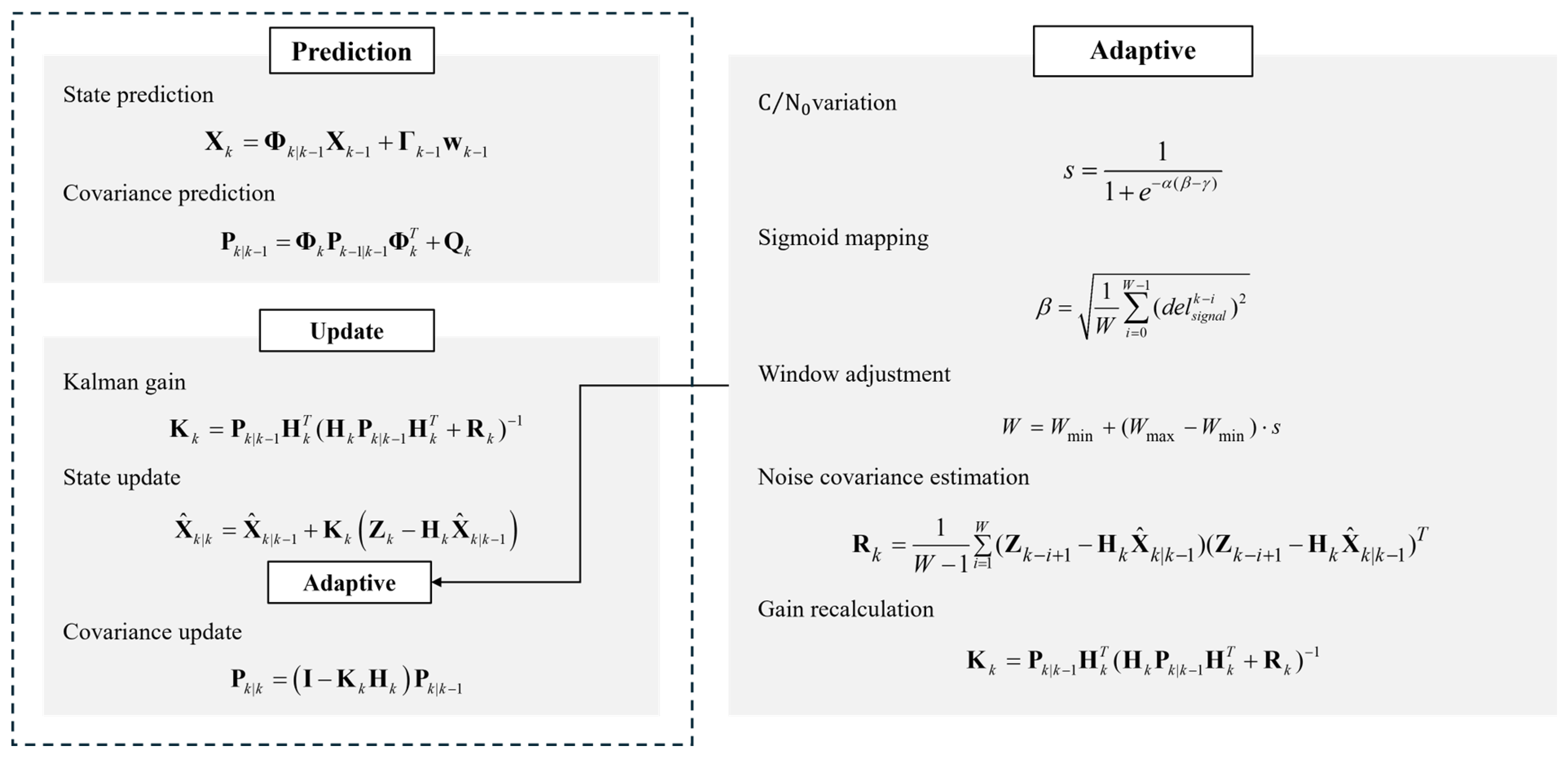
The algorithm flowchart for this paper is shown in Figure 2. For traditional Kalman filter tight combinations, there are only two steps: prediction and update. In the prediction phase, the current state estimate is derived using the state estimate from the previous time step and the control input. In the update phase, the state estimate obtained in the prediction phase is updated by incorporating the current observation data, resulting in a more accurate state estimate. For the update step, this paper introduces an adaptive step after calculating $K_k$ and ${\widehat{X}}_{k|k}$, using a dynamic sliding window method to adaptively update the $R_k$ and $K_k$ matrices for the next time step’s prediction and update, thereby improving the algorithm’s accuracy.

3. Results

3.1. Simulation Scenario and GNSS Observation Characteristics

3.1.1. Simulation Scenario Settings

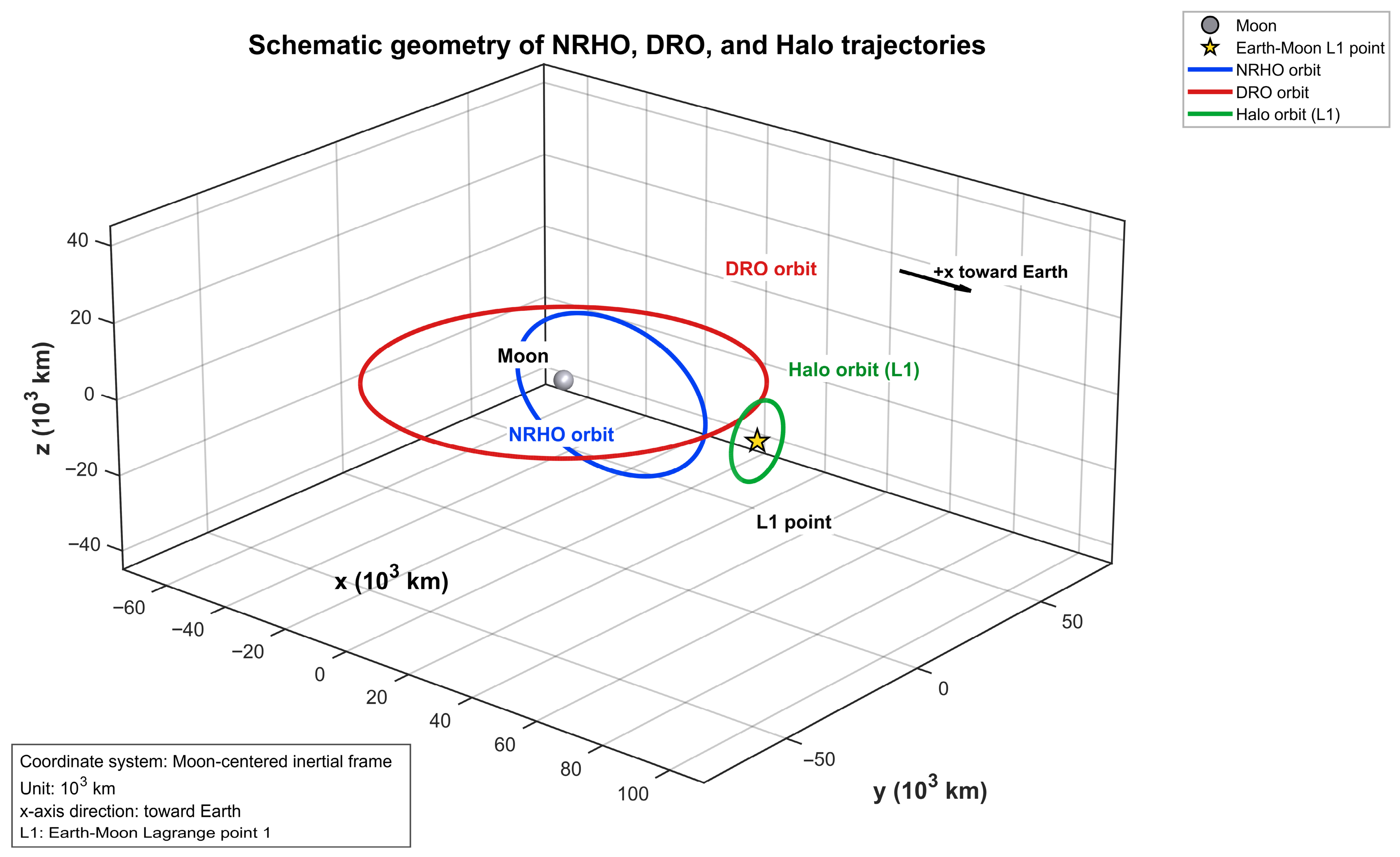
Figure 3 shows the schematic geometry of the three representative trajectories in a Moon-centered inertial frame [1,3,5]. The positive x-axis approximately points toward Earth, and the coordinate unit is 10³ km. In this representation, the DRO surrounds the Moon with a relatively large spatial scale, the NRHO is located in the near-lunar region with a pronounced three-dimensional geometry, and the Halo orbit is located near the Earth–Moon L1 point along the Earth-facing direction. This schematic view is used to illustrate the relative geometric relationship among the three trajectories considered in the simulation.

The total duration of each simulation arc is 20 days, with a sampling interval of 600 s. The initial position error is set to 500 m, the initial velocity error is set to 0.01 m/s, and the nominal pseudo-range observation error is set to 5 m. These settings are chosen to be broadly consistent with representative cislunar navigation and orbit-determination studies [10,11,46]. The orbital dynamics are propagated in the geocentric inertial frame, while the simulation results and error statistics are expressed in the Earth-centered, Earth-fixed (ECEF) frame. During the simulation, pure dynamic propagation is used as a reference baseline, while the main comparative analysis focuses on the conventional SPP tightly coupled solution and four adaptive schemes with fixed window sizes of 5, 10, and 15, and a dynamically adjusted window size, respectively.

3.1.2. GNSS Visibility, DOP, and $C/N_0$ Characteristics

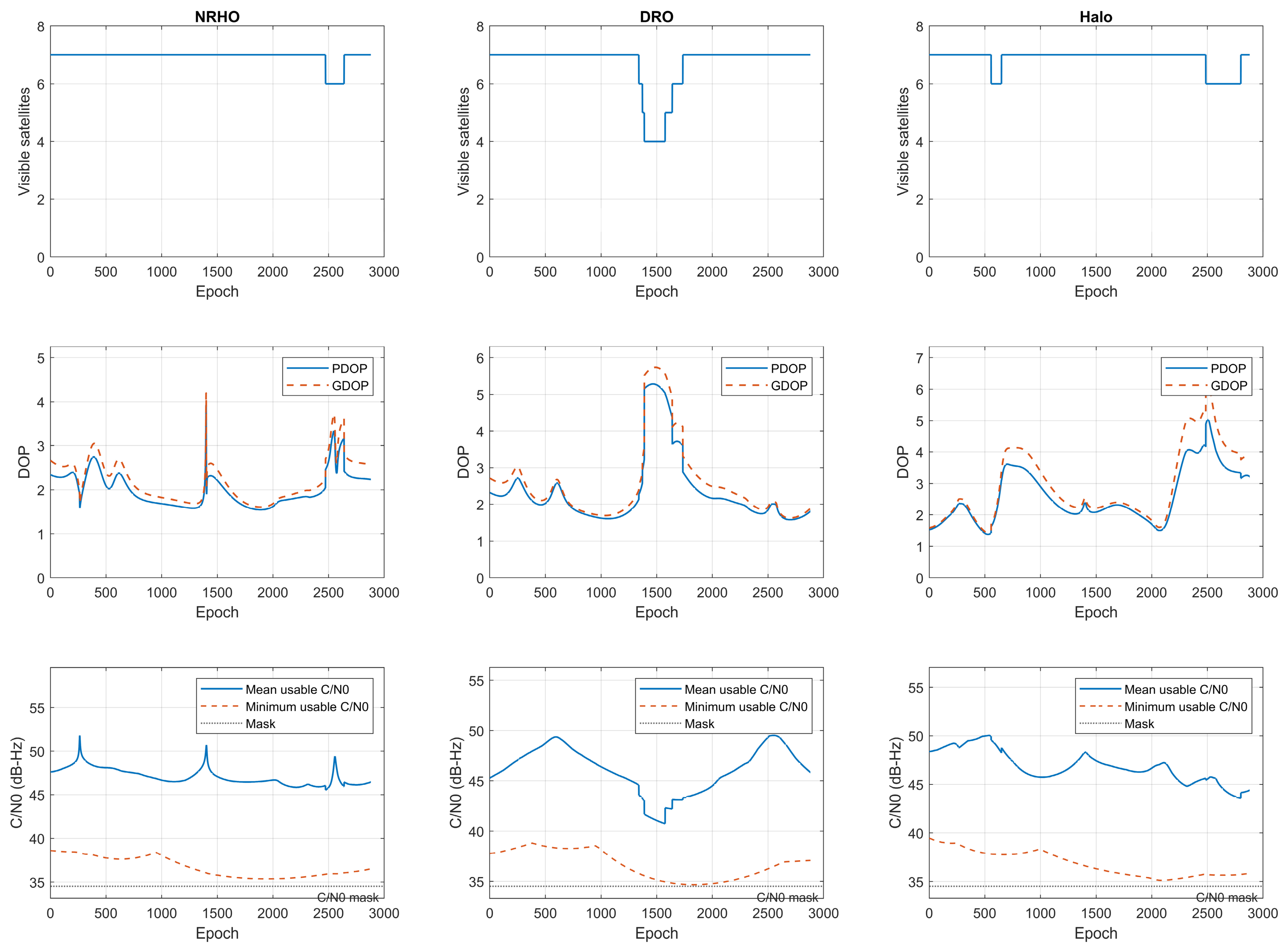
Before evaluating the orbit-determination performance, the GNSS observation conditions of the three representative trajectories were analyzed using satellite visibility, dilution of precision (DOP), and equivalent $C/N_0$. Since the simulated trajectory files do not contain measured $C/N_0$ values, an equivalent $C/N_0$ indicator was generated using a simplified geometry-dependent link-quality model. In this model, the signal quality is affected by the inter-spacecraft distance and the transmitter off-boresight angle. A link was counted as usable only when the equivalent $C/N_0$ exceeded the adopted threshold and the off-boresight angle was within the allowable range. This analysis provides a simplified but physically interpretable description of time-varying GNSS signal availability in Earth–Moon space.

Figure 4 shows the GNSS visibility, DOP, and equivalent $C/N_0$ characteristics for the NRHO, DRO, and Halo trajectories. The three trajectories generally maintain about seven usable observation links, although short-term visibility reductions occur in several local intervals, especially for the DRO trajectory around epochs 1400–1700. The DOP variations are consistent with the visibility changes: The position dilution of precision (PDOP) and geometric dilution of precision (GDOP) increase when the number of usable links decreases or the observation geometry becomes less favorable. For the Halo trajectory, several local fluctuations can also be observed in the DOP and equivalent $C/N_0$ series, indicating that its observation geometry and signal quality are not constant over the simulation arc. The mean usable $C/N_0$ remains above the adopted threshold for all three trajectories, while the minimum usable $C/N_0$ stays closer to the threshold and varies with time. These results indicate that the Earth–Moon GNSS observation environment is usable over most epochs but remains time-varying in both geometry and signal quality.

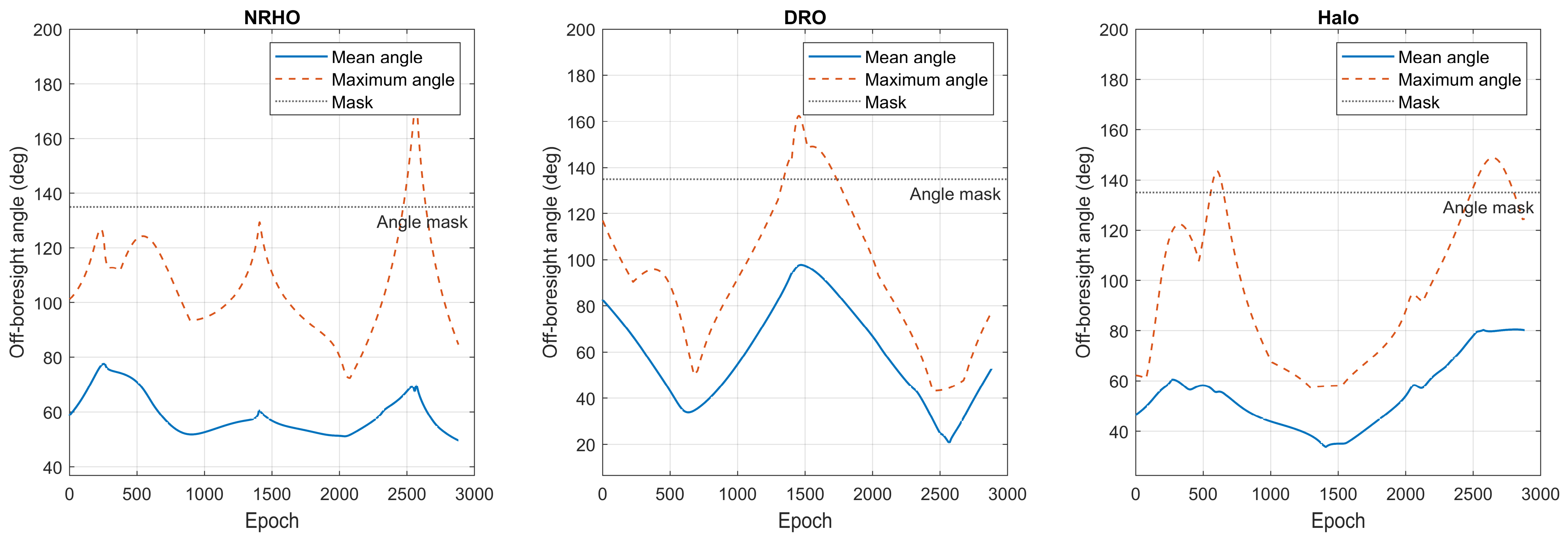
To further explain the signal-quality variation, Figure 5 shows the transmitter off-boresight angle characteristics. The intervals with reduced visibility and increased DOP generally correspond to periods when the maximum off-boresight angle approaches or exceeds the angular mask, such as the local degradation intervals of the NRHO, DRO, and Halo trajectories. This indicates that the changes in usable satellite number and equivalent $C/N_0$ are closely related to the spacecraft–satellite geometry and antenna-pattern-related emission conditions.

Overall, the visibility, DOP, equivalent $C/N_0$, and off-boresight-angle results show that the GNSS observation environment in Earth–Moon space is practically usable but clearly time-varying. The local visibility reductions, DOP increases, and $C/N_0$ fluctuations indicate that a fixed-window strategy may be insufficient to balance stability and responsiveness. These results further support the use of $C/N_0$ variation as the input for the proposed adaptive sliding-window regulation strategy.

3.2. Error Analysis Under Various Trajectories

3.2.1. Position Error Comparison

To evaluate the proposed method, orbit-determination experiments were conducted for three representative Earth–Moon trajectories. Since the methodological contribution of this work lies in improving the conventional tightly coupled framework through adaptive window regulation, the following analysis focuses primarily on the comparison between the proposed dynamic-window method, the fixed-window adaptive schemes, and the conventional SPP tightly coupled solution.

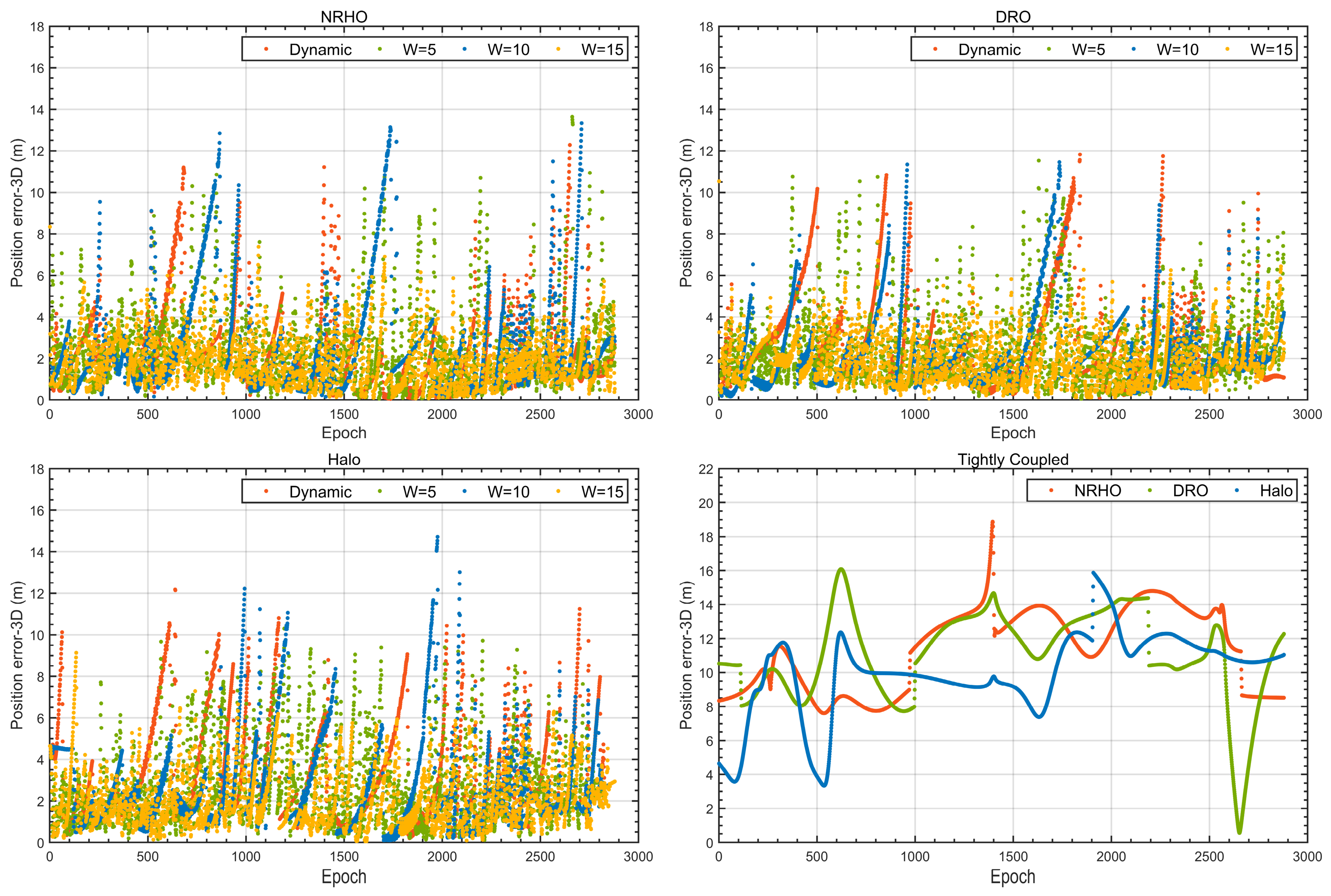
As shown in Figure 6, the conventional tightly coupled method already constrains the position error effectively by introducing SPP observations into the dynamic propagation process. However, its performance remains limited by fixed statistical parameters, which cannot fully accommodate the time-varying observation quality in Earth–Moon space. In contrast, the adaptive sliding-window schemes maintain the position error within a lower range and produce smoother error evolution over the full propagation arc. Among them, the dynamic-window method provides the most stable behavior, indicating that adaptive covariance adjustment improves the balance between dynamic prediction and measurement correction under time-varying observation conditions.

Compared with the conventional tightly coupled method, the adaptive sliding-window schemes consistently yield lower position errors and smoother error evolution over the full propagation arc. This confirms that, beyond the basic benefit of measurement-aided correction, adaptive regulation of the observation-noise statistics further enhances the capability of the filter to suppress long-term error accumulation.

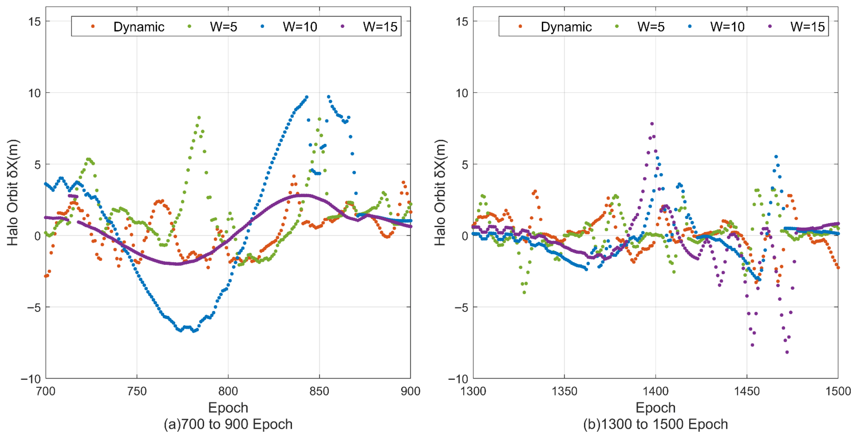
Figure 7 further illustrates the effect of window length on local error behavior by taking the x-direction error of the Halo orbit as an example. In different ephemeris intervals, the fixed-window schemes exhibit different advantages and disadvantages. For example, during epochs 700–900, the errors with W = 5 and W = 10 are noticeably larger than those with W = 15 and the dynamic window, whereas during epochs 1300–1500, the errors with W = 10 and W = 15 become larger, while W = 5 and the dynamic window perform better. These results indicate that no single fixed window can maintain optimal performance over all orbital phases. By contrast, the dynamic-window scheme provides consistently lower errors in both intervals, demonstrating its superior adaptability to phase-dependent changes in dynamics and observation quality.

Overall, the dynamic-window adaptive method achieves the best position-estimation performance among all compared schemes for NRHO, DRO, and Halo orbits. It not only suppresses long-term error accumulation but also reduces local fluctuation amplitudes in characteristic orbital segments.

3.2.2. Velocity Error Comparison

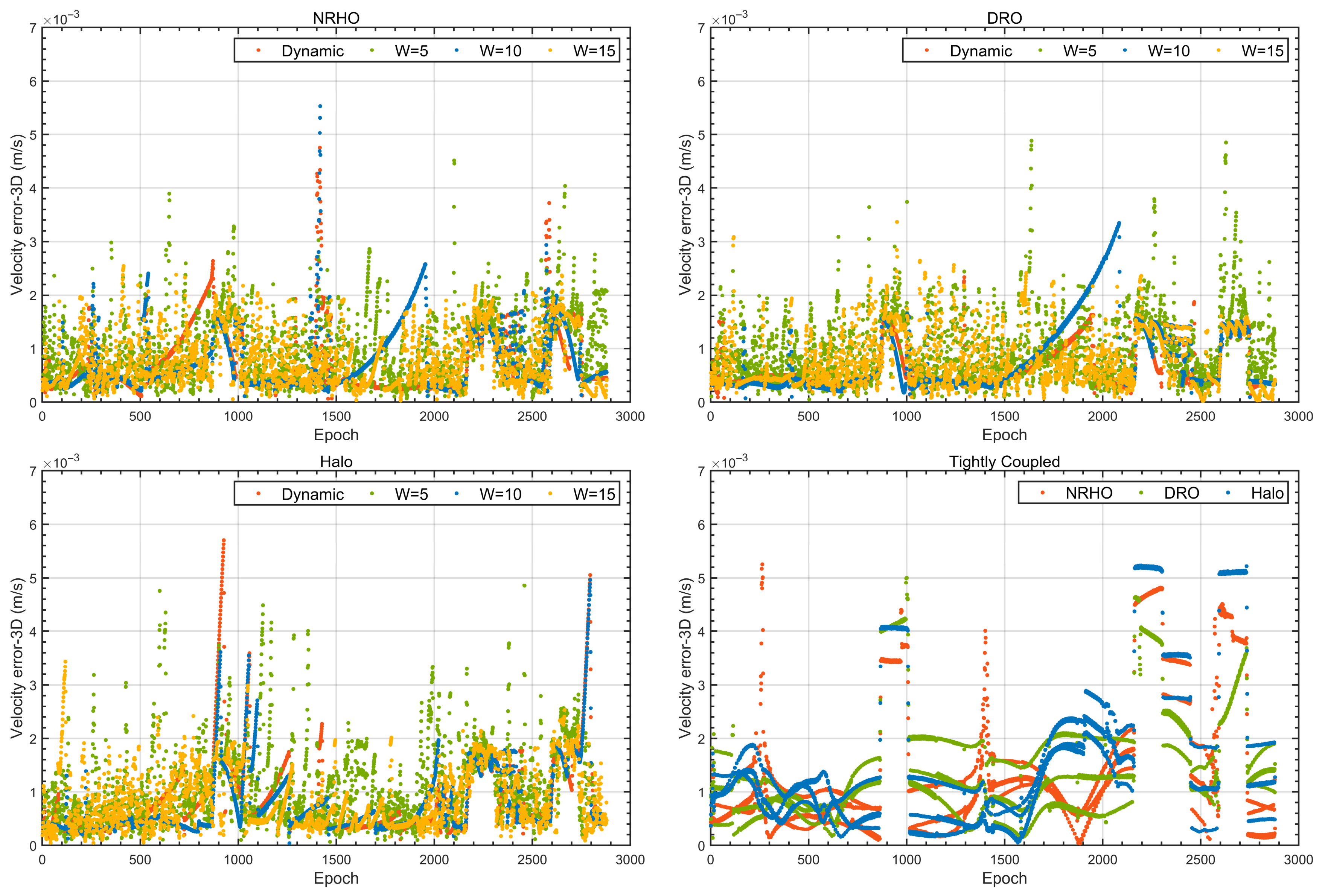
Figure 8 compares the velocity errors of different methods for the three representative Earth–Moon trajectories. The conventional SPP tightly coupled method can already maintain the velocity error at the 10⁻³–10⁻² m/s level, indicating that measurement updates are effective in constraining velocity estimation. However, its error curves still contain noticeable high-frequency oscillations, especially in orbital segments where the observation quality or model mismatch changes rapidly.

The adaptive schemes further improve the velocity-estimation performance by mitigating these oscillations. Compared with the conventional tightly coupled method, the fixed-window adaptive methods produce smoother velocity-error curves and generally lower error amplitudes. Nevertheless, their performance still depends on the selected window length. A short window improves responsiveness but may amplify local fluctuations, whereas a long window enhances smoothing at the cost of slower adaptation to abrupt changes.

Among all schemes, the dynamic-window method provides the most balanced performance. Its velocity error remains at the lowest overall level across the three orbit types, while the corresponding curves are smoother and less oscillatory than those of the comparison methods. This result is consistent with the position-error analysis and confirms that adaptive window adjustment is beneficial not only for position correction but also for the stabilization of velocity estimation.

3.3. RMS Comparison of Positioning Errors

3.3.1. Overall RMS Comparison Among Different Orbits

To quantify the differences among the compared methods more clearly, the RMS values of the position errors are further calculated. Since all adaptive schemes are developed on top of the conventional SPP tightly coupled framework, the following discussion emphasizes the improvement of each adaptive method relative to the conventional tightly coupled solution rather than to pure dynamic propagation.

As shown in

Table 1. RMS position errors for the NRHO.

Resolution Method	Position Error RMS/m
	X	Y	Z
Conventional SPP tightly coupled	6.05	5.96	7.94
W = 5	1.94	1.78	1.37
W = 10	2.32	2.32	1.78
W = 15	1.91	1.96	1.09
Dynamic window	1.43	1.40	0.97

, for the NRHO case, the conventional SPP tightly coupled method yields RMS position errors of 6.05 m, 5.96 m, and 7.94 m in the X, Y, and Z directions, respectively. The dynamic-window method reduces these values to 1.43 m, 1.400 m, and 0.97 m, corresponding to reductions of 76.4%, 76.5%, and 87.8%, respectively. In terms of the three-dimensional RMS position error, the value is reduced from 6.65 m for the conventional tightly coupled solution to 1.27 m for the dynamic-window solution, representing an overall improvement of 80.9%. Compared with the fixed-window adaptive schemes, the dynamic-window method also provides the most balanced performance among the three axes, indicating that it can better reconcile responsiveness and statistical stability under varying observation conditions.

A similar trend can be observed for the DRO case in

Table 2. RMS position errors for the DRO.

Resolution Method	Position Error RMS/m
	X	Y	Z
Conventional SPP tightly coupled	6.57	6.56	6.58
W = 5	1.70	1.75	1.66
W = 10	2.10	2.08	0.63
W = 15	2.35	2.30	1.24
Dynamic window	1.40	1.48	0.93

. The conventional SPP tightly coupled solution gives RMS errors of 6.57 m, 6.56 m, and 6.58 m in the X, Y, and Z directions, respectively, whereas the dynamic-window method reduces them to 1.40 m, 1.48 m, and 0.93 m. These correspond to reductions of 78.8%, 77.5%, and 85.8%, respectively. The three-dimensional RMS position error is reduced from 6.57 m to 1.27 m, giving an overall improvement of 80.4%. Although one fixed-window scheme may perform slightly better in an individual component, the dynamic-window method again provides the best overall balance across the three axes, which confirms its stronger adaptability under the DRO trajectory.

As shown in

Table 3. RMS position errors for the Halo orbit.

Resolution Method	Position Error RMS/m
	X	Y	Z
Conventional SPP tightly coupled	6.24	6.30	5.18
W = 5	2.18	2.08	1.18
W = 10	2.42	2.30	1.44
W = 15	2.81	2.82	1.02
Dynamic window	1.57	1.64	1.09

, for the Halo orbit, the conventional SPP tightly coupled method yields RMS errors of 6.24 m, 6.30 m, and 5.18 m in the X, Y, and Z directions, respectively. The corresponding values for the dynamic-window method are 1.57 m, 1.64 m, and 1.09 m, which correspond to reductions of 74.8%, 73.9%, and 79.0%. The three-dimensional RMS position error decreases from 5.91 m to 1.44 m, corresponding to an overall improvement of 75.4%. Although certain fixed-window schemes are competitive in individual directions, the dynamic-window method still provides the most balanced overall solution, indicating that its advantage is maintained under different orbital geometries.

Taken together, the RMS results for NRHO, DRO, and Halo orbits consistently show that the proposed dynamic-window strategy significantly improves upon the conventional tightly coupled solution. Relative to the conventional SPP tightly coupled method, the three-dimensional RMS position error is reduced by 80.9% for NRHO, 80.4% for DRO, and 75.4% for Halo. Figure 9 summarizes the relative gains of the fixed-window and dynamic-window schemes and shows that the dynamic-window method consistently provides the largest overall improvement across all three representative trajectories. This pattern indicates that the proposed $C/N_0$-driven dynamic window regulation enables the observation-noise adaptation to better track actual signal-quality variation, thereby providing a more effective correction mechanism for suppressing long-arc error accumulation than fixed-window schemes.

3.3.2. Comparison with Representative Adaptive Filtering Methods

To further evaluate the proposed method against a representative adaptive filtering strategy, a fading Kalman filter (FADE-KF) was added as an additional benchmark. FADE-KF improves filter responsiveness by inflating the predicted covariance through a fading factor. For a fair comparison, the conventional SPP tightly coupled solution, FADE-KF, and the proposed dynamic-window method were tested using the same dynamic model, measurement model, initial error settings, and nominal observation-noise conditions. The RMS position errors in the X, Y, and Z directions are summarized in

Table 4. RMS position error comparison with FADE-KF for the NRHO, DRO, and Halo orbits.

Trajectory	Resolution Method	Position Error RMS/m
		X	Y	Z
NRHO	Conventional SPP tightly coupled	6.05	5.96	7.94
	FADE-KF	6.84	7.23	7.25
	Dynamic window	1.43	1.40	0.97
DRO	Conventional SPP tightly coupled	6.57	6.56	6.58
	FADE-KF	8.90	8.65	7.04
	Dynamic window	1.40	1.48	0.93
Halo	Conventional SPP tightly coupled	6.24	6.30	5.18
	FADE-KF	8.43	8.85	5.46
	Dynamic window	1.57	1.64	1.09

.

As shown in Table 4, FADE-KF does not consistently outperform the conventional SPP tightly coupled solution. Its RMS errors are slightly larger than those of the conventional solution for most trajectories and position components. This is mainly because FADE-KF improves filter responsiveness by inflating the predicted covariance, which increases the influence of current observations. Under weak and time-varying Earth–Moon GNSS observation conditions, however, this mechanism may also increase the sensitivity of the filter to noisy pseudo-range updates.

By contrast, the proposed dynamic-window method still achieves lower RMS errors than both the conventional solution and FADE-KF. This result further indicates that the $C/N_0$-driven dynamic-window regulation provides a more targeted adaptation to time-varying signal quality than general covariance inflation.

3.4. Sensitivity Analysis of Dynamic-Window Parameters

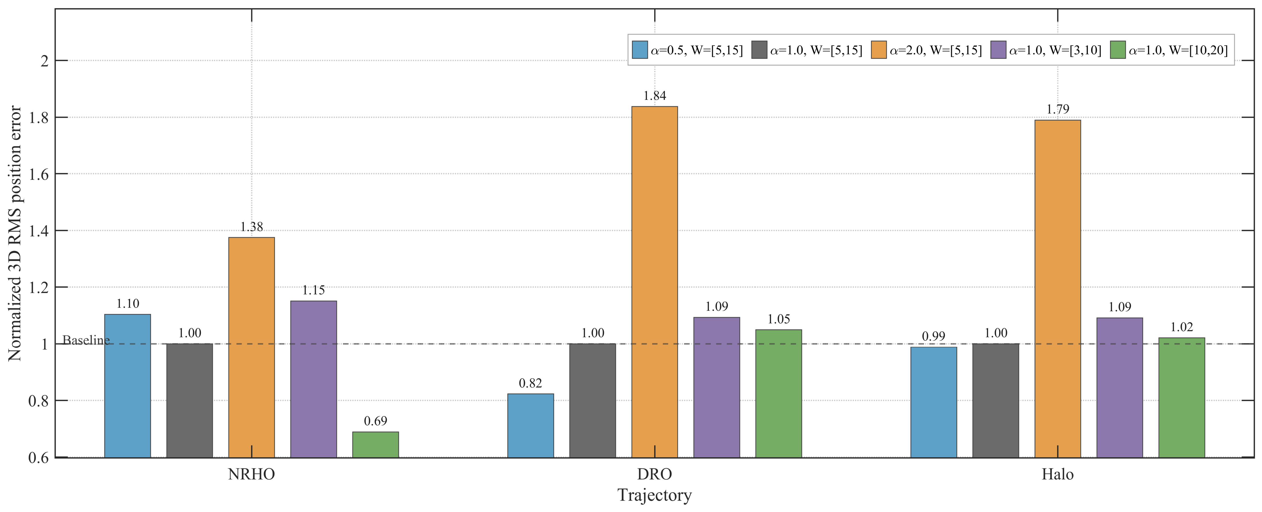
To evaluate the influence of the key parameters in the dynamic-window regulation strategy, a normalized sensitivity analysis was conducted for the sigmoid sensitivity coefficient α and the allowable window-length range. The adopted setting, α = 1.0 and W = [5, 15], was selected as a stable and competitive configuration based on preliminary tests, and was kept unchanged for all three trajectories in the comparative experiments. For each trajectory, the 3D RMS position error obtained under each parameter setting was normalized by the corresponding result of α = 1.0 and W = [5, 15]. The normalized results are shown in Figure 10.

As shown in Figure 10, the estimation performance is affected by both α and the window-length range. For the sensitivity coefficient, increasing α to 2.0 leads to a clear increase in the normalized error for all three trajectories. The increase is particularly evident for the DRO and Halo trajectories, where the normalized errors reach 1.84 and 1.79, respectively. This indicates that an excessively large sensitivity coefficient may make the window adjustment too responsive to local signal variations, resulting in less stable covariance estimation. By contrast, reducing α to 0.5 produces different effects for different trajectories. The normalized error slightly increases for NRHO, decreases for DRO, and remains close to the baseline for Halo, indicating that a smaller sensitivity coefficient does not provide a consistent improvement across all trajectory types.

The influence of the window-length range also varies among the three trajectories. For NRHO, the longer window range W = [10, 20] gives the lowest normalized error, suggesting that stronger smoothing is beneficial for this trajectory. For DRO and Halo, however, the same window range only produces limited improvement or remains close to the baseline. The shorter range W = [3, 10] results in normalized errors larger than 1.0 for all three trajectories, indicating that an overly short covariance-estimation window may reduce statistical stability.

Overall, the sensitivity analysis shows that the parameter influence is trajectory-dependent. No single alternative setting provides consistent improvement for all three trajectories. The adopted setting α = 1.0 and W = [5, 15] therefore provides a balanced configuration for the NRHO, DRO, and Halo cases, while maintaining stable performance under moderate parameter variations.

3.5. Error and Recovery Under SPP Signal Loss

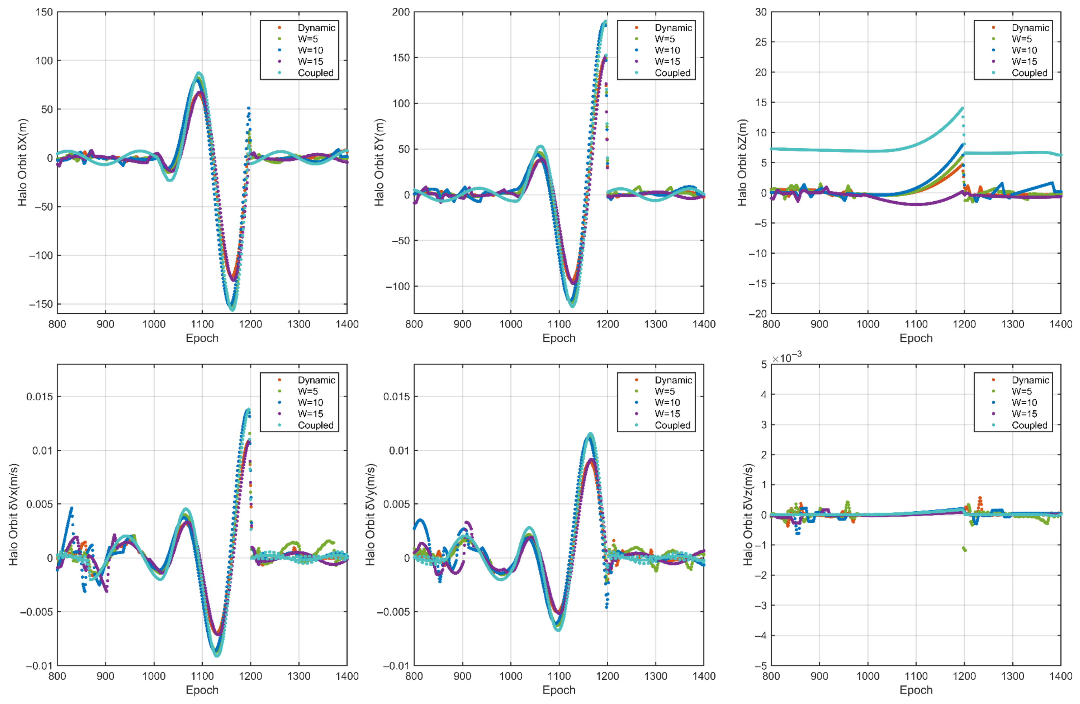
To evaluate the prediction performance during observation outages and the recovery capability after signal restoration, a complete SPP interruption lasting 200 epochs was introduced into the Halo-orbit simulation, from epoch 1000 to epoch 1200. During this interval, all methods relied solely on dynamic propagation without measurement updates. Figure 11 shows the position and velocity errors of the compared methods under this interruption scenario.

As shown in Figure 11, the errors of all methods increase during the interruption interval, but the growth rates differ substantially. The conventional tightly coupled method and the adaptive schemes with short fixed windows exhibit relatively larger divergence, whereas the W = 15 and dynamic-window schemes maintain smaller errors throughout the outage. This indicates that a larger effective smoothing scale is advantageous for suppressing error growth when the filter temporarily operates in a prediction-dominated mode.

After signal restoration at epoch 1200, all adaptive schemes recover faster than the conventional tightly coupled solution. Among them, the dynamic-window method exhibits the fastest re-convergence, with the error returning to the pre-interruption level within a shorter interval. This behavior indicates that dynamic window regulation improves not only outage suppression but also the ability of the filter to rapidly readapt to restored observations.

To quantify these differences more clearly, RMS values of the position errors were further computed for both the interruption-centered interval and the full simulation arc.

Table 5. RMS position errors for the Halo orbit in the interruption-centered interval (Epoch 800–1400).

Resolution Method	Position Error RMS/m
	X	Y	Z
Conventional SPP tightly coupled	43.63	47.12	7.66
W = 5	42.03	46.13	1.36
W = 10	41.87	47.64	1.83
W = 15	34.60	35.79	0.92
Dynamic window	33.61	36.56	1.04

and

Table 6. RMS position errors for the Halo orbit over the full arc under signal interruption.

Resolution Method	Position Error RMS/m
	X	Y	Z
Conventional SPP tightly coupled	20.72	22.07	5.42
W = 5	19.27	21.12	1.26
W = 10	19.22	21.84	1.23
W = 15	15.93	16.48	0.97
Dynamic window	15.38	16.73	0.85

summarize the corresponding results for epochs 800–1400 and for all epochs, respectively.

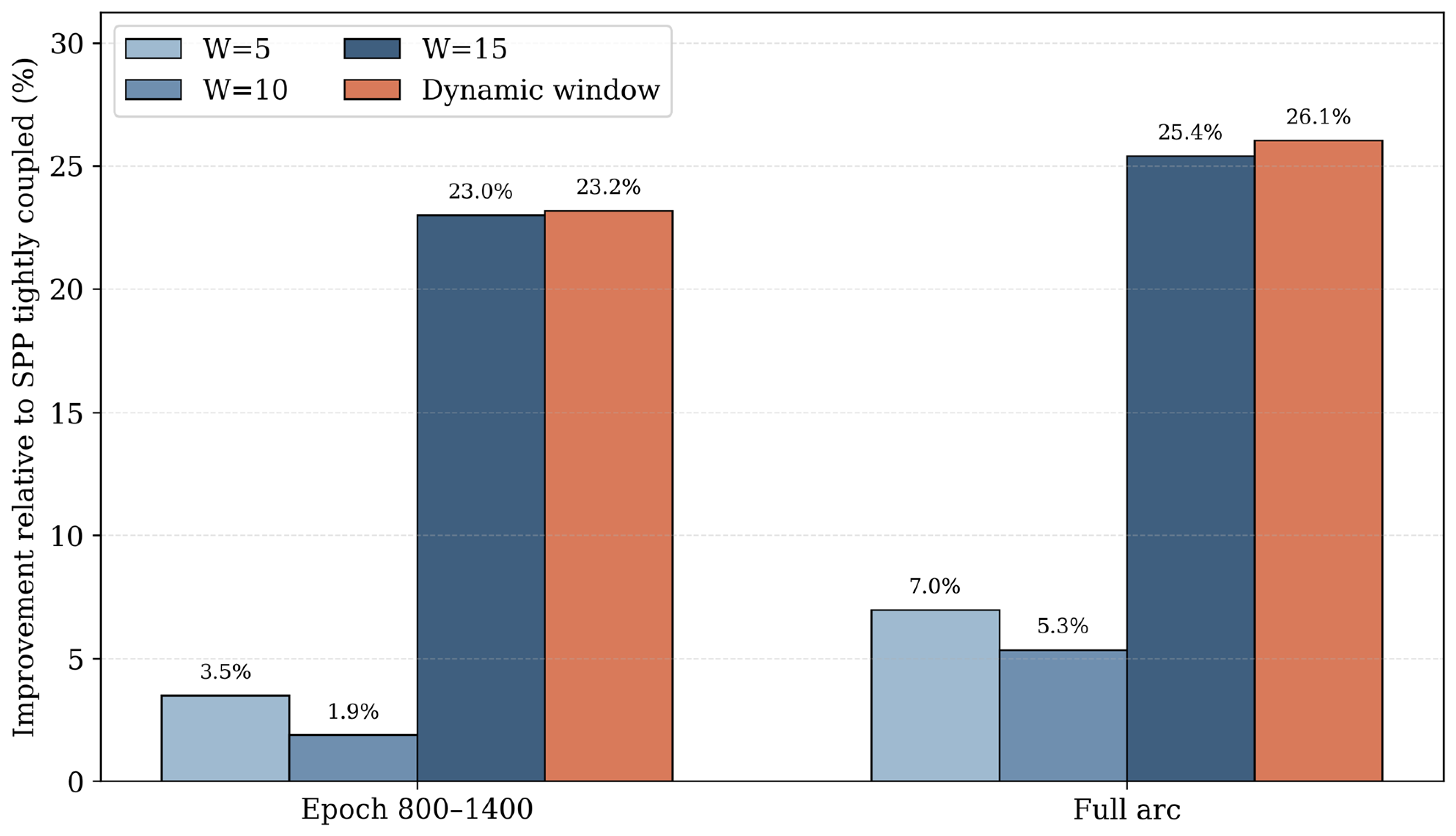
As shown in Table 5, within the interruption-centered interval, the conventional SPP tightly coupled method yields RMS position errors of 43.63 m, 47.12 m, and 7.66 m in the X, Y, and Z directions, respectively. The dynamic-window method reduces these values to 33.61 m, 36.56 m, and 1.04 m, corresponding to reductions of 23.0%, 22.4%, and 86.4%, respectively. In terms of the three-dimensional RMS position error, the value decreases from 32.80 m to 23.74 m, which corresponds to an overall improvement of 23.2%.

Among the fixed-window methods, W = 15 performs better than W = 5 and W = 10, indicating that stronger smoothing is advantageous in the presence of outage-induced error growth. The dynamic-window method achieves the lowest RMS values in the X and Y directions while maintaining vertical accuracy close to that of W = 15. This suggests that adaptive window adjustment can preserve the stability advantage of a relatively large window while retaining greater flexibility under changing conditions.

Table 6 presents the full-arc RMS statistics and therefore reflects the overall estimation quality over the entire simulation period rather than only the local behavior around the interruption interval. The conventional SPP tightly coupled method yields RMS position errors of 20.72 m, 22.07 m, and 5.42 m in the X, Y, and Z directions, whereas the dynamic-window method reduces them to 15.38 m, 16.73 m, and 0.85 m. These correspond to reductions of 25.8%, 24.2%, and 84.2%, respectively. The three-dimensional RMS position error decreases from 16.071 m to 10.989 m, corresponding to an overall improvement of 26.1%.

Figure 12 summarizes the relative reduction in the 3D RMS position error under the simulated signal-interruption scenario. Unlike the nominal-observation case, the short-window schemes provide only limited improvement during the interruption-centered interval, whereas the W = 15 and dynamic-window schemes achieve substantially larger gains. Over the full arc, the dynamic-window method again provides the largest overall improvement, indicating that it not only suppresses error growth during observation loss but also maintains better long-term consistency after signal recovery. Overall, relative to the conventional tightly coupled solution, the proposed method reduces the three-dimensional RMS position error by 23.2% in the interruption-centered interval and by 26.1% over the full arc.

4. Conclusions

This paper investigated GNSS SPP-aided orbit determination in Earth–Moon space within a tightly coupled Kalman filtering framework. To improve robustness under weak, intermittent, and time-varying observation conditions, a dynamic sliding-window strategy was introduced to adaptively regulate the observation-noise statistics during filtering. Rather than modifying the basic state-space formulation of the tightly coupled filter, the proposed method improves the characterization of observation uncertainty during the update stage through $C/N_0$-driven adjustment of the effective window length.

Simulation experiments were carried out for three representative cislunar trajectories, namely NRHO, DRO, and Halo orbits. The supplementary analysis of GNSS visibility, DOP, and signal-quality characteristics further confirmed that the observation geometry and received signal quality vary significantly among different cislunar trajectories, which supports the need for adaptive observation-noise regulation. Relative to the conventional SPP tightly coupled solution, the proposed dynamic-window method reduced the three-dimensional RMS position error from 6.65 m to 1.27 m for NRHO, from 6.57 m to 1.27 m for DRO, and from 5.91 m to 1.44 m for Halo, corresponding to overall improvements of 80.9%, 80.4%, and 75.4%, respectively. In the individual X, Y, and Z components, the corresponding error reductions were generally in the range of 74–88%, indicating that the proposed method maintained strong and balanced performance under different orbital geometries.

The comparison with representative adaptive filtering methods showed that the proposed dynamic-window strategy achieved more balanced accuracy and robustness under time-varying GNSS observation conditions. In addition, the sensitivity analysis of the dynamic-window parameters indicated that the selected parameter configuration provides a reasonable trade-off between smoothing stability and responsiveness to signal-quality variations.

Under a simulated 200-epoch GNSS signal interruption in the Halo-orbit case, the proposed method also showed stronger robustness than the conventional tightly coupled method. The three-dimensional RMS position error was reduced by 23.2% in the interruption-centered interval and by 26.1% over the full arc, while faster post-outage re-convergence was also observed. These results demonstrate that the proposed strategy improves not only nominal orbit-determination accuracy but also outage resilience and recovery capability under degraded observation conditions.

Overall, the main contribution of this work is to demonstrate that dynamic window regulation can further and significantly improve the conventional tightly coupled orbit-determination framework under time-varying GNSS observation conditions in Earth–Moon space. Future work will focus on validation under more realistic cislunar observation scenarios, improved perturbation modeling, and integration with additional navigation information sources, such as inter-satellite links and ground-based tracking data.

References

1. Folta, D.C.; Pavlak, T.A.; Haapala, A.F.; Howell, K.C.; Woodard, M.A. Earth-Moon libration point orbit stationkeeping: Theory, modeling, and operations. Acta Astronaut. 2014, 94, 421–433. [Google Scholar] [CrossRef]
2. Zhang, Z.; Hou, X. Transfer orbits to the Earth-Moon triangular libration points. Adv. Space Res. 2015, 55, 2899–2913. [Google Scholar] [CrossRef]
3. Farquhar, R.W.; Dunham, D.W.; Guo, Y.; McAdams, J.V. Utilization of libration points for human exploration in the Sun-Earth-Moon system and beyond. Acta Astronaut. 2004, 55, 687–700. [Google Scholar] [CrossRef]
4. Sesta, A.; Durante, D.; Boscagli, G.; Cappuccio, P.; di Benedetto, M.; di Stefano, I.; Plumaris, M.K.; Racioppa, P.; Iess, L.; Giordano, P.; et al. ATLAS: Orbit Determination and Time Transfer for a Lunar Radio Navigation System. Navig. J. Inst. Navig. 2025, 72, navi.701. [Google Scholar] [CrossRef]
5. Hou, X.; Liu, L.; Tang, J. Station-keeping of small amplitude motions around the collinear libration point in the real Earth-Moon system. Adv. Space Res. 2011, 47, 1127–1134. [Google Scholar] [CrossRef]
6. Tan, B.; Yuan, Y.; Ai, Q.; Zha, J. Real-Time Multi-GNSS Precise Orbit Determination Based on the Hourly Updated Ultra-Rapid Orbit Prediction Method. Remote Sens. 2022, 14, 4412. [Google Scholar] [CrossRef]
7. Gao, Y.; Wang, Z.; Zhang, Y. Low thrust Earth–Moon transfer trajectories via lunar capture set. Astrophys. Space Sci. 2019, 364, 219. [Google Scholar] [CrossRef]
8. Mcelreath, J.; Majji, M. Lunar Orbit Determination Sensitivity Analysis with Reference to Observational Geometry. J. Astronaut. Sci. 2023, 70, 39. [Google Scholar] [CrossRef]
9. Kulkarni, J.E.; Campbell, M.E.; Dullerud, G.E. Stabilization of Spacecraft Flight in Halo Orbits: An Hinfty Approach. IEEE Trans. Control Syst. Technol. 2006, 14, 572–578. [Google Scholar] [CrossRef]
10. Vouch, O.; Morichi, L.; Zocca, S.; Minetto, A.; Dovis, F. GNSS Precise Point Positioning in Cislunar Space: A Study on Regularized Least Squares and Availability. In Proceedings of the 2025 IEEE/ION Position, Location and Navigation Symposium (PLANS), Salt Lake City, UT, USA, 28 April 2025; IEEE: New York, NY, USA, 2025; pp. 1014–1025. [Google Scholar]
11. Wang, D.; Xu, T.; Li, M.; Shi, Y. Navigation performance analysis of Earth–Moon spacecraft using GNSS, INS, and star tracker. Satell. Navig. 2024, 5, 16. [Google Scholar] [CrossRef]
12. Iiyama, K.; Bhamidipati, S.; Gao, G. Precise Positioning and Timekeeping in a Lunar Orbit via Terrestrial GPS Time-Differenced Carrier-Phase Measurements. Navig. J. Inst. Navig. 2024, 71, navi.635. [Google Scholar] [CrossRef]
13. He, B.; Xu, T.; Wang, D.; Liu, Y. Autonomous Orbit Determination for Lunar Navigation Constellation Using Low Earth Orbit Satellites. Adv. Space Res. 2026, 77, 6659–6674. [Google Scholar] [CrossRef]
14. Chen, S.; Li, S.; Pu, J.; Xu, Y.; Wang, W. Autonomous Orbit Determination of LLO Satellite Using DRO-LLO Links and Lunar Laser Ranging. Aerospace 2025, 12, 576. [Google Scholar] [CrossRef]
15. Akhlaghi, S.; Zhou, N.; Huang, Z. Adaptive Adjustment of Noise Covariance in Kalman Filter for Dynamic State Estimation. In Proceedings of the 2017 IEEE Power & Energy Society General Meeting, Chicago, IL, USA, 16–20 July 2017; pp. 1–5. [Google Scholar]
16. Ge, Q.; Ma, Z.; Li, J.; Yang, Q.; Lu, Z.; Li, H. Adaptive cubature Kalman filter with the estimation of correlation between multiplicative noise and additive measurement noise. Chin. J. Aeronaut. 2022, 35, 40–52. [Google Scholar] [CrossRef]
17. Wang, Z.; Hou, X.; Dan, Z.; Fang, K. Adaptive Kalman filter based on integer ambiguity validation in moving base RTK. GPS Solut. 2023, 27, 34. [Google Scholar] [CrossRef]
18. Kruse, T.; Griebel, T.; Graichen, K. Adaptive Kalman Filtering: Measurement and Process Noise Covariance Estimation Using Kalman Smoothing. IEEE Access 2025, 13, 11863–11875. [Google Scholar] [CrossRef]
19. Erkec, T.Y.; Hajiyev, C. Estimation of the Relative States of Satellite Formation Flights Using the Adaptive Extended Kalman Filter. Gyroscopy Navig. 2023, 14, 154–165. [Google Scholar] [CrossRef]
20. Kang, C.H.; Kim, S.Y.; Park, C.G. Global navigation satellite system interference tracking and mitigation based on an adaptive fading Kalman filter. IET Radar Sonar Navig. 2015, 9, 1030–1039. [Google Scholar] [CrossRef]
21. Huang, G.; Zhang, Q. Real-time estimation of satellite clock offset using adaptively robust Kalman filter with classified adaptive factors. GPS Solut. 2012, 16, 531–539. [Google Scholar] [CrossRef]
22. Cheng, S.; Cheng, J.; Zang, N.; Zhang, Z.; Chen, S. A Sequential Student’s t-Based Robust Kalman Filter for Multi-GNSS PPP/INS Tightly Coupled Model in the Urban Environment. Remote Sens. 2022, 14, 5878. [Google Scholar] [CrossRef]
23. Wang, D.; Zhang, H. A Multi-Step Pseudo-Measurement Adaptive Kalman Filter Based on Filtering Performance Evaluation and Its Application in the INS/GNSS Navigation System. Remote Sens. 2024, 16, 926. [Google Scholar] [CrossRef]
24. Jiao, H.; Tao, X.; Chen, L.; Zhou, X.; Ju, Z. GNSS/5G Joint Position Based on Weighted Robust Iterative Kalman Filter. Remote Sens. 2024, 16, 1009. [Google Scholar] [CrossRef]
25. Wang, R.; Becker, D.; Hobiger, T. Stochastic Modeling with Robust Kalman Filter for Real-Time Kinematic GPS Single-Frequency Positioning. GPS Solut. 2023, 27, 153. [Google Scholar] [CrossRef]
26. Jin, B.; Guo, J.; He, D.; Guo, W. Adaptive Kalman Filtering Based on Optimal Autoregressive Predictive Model. GPS Solut. 2017, 21, 307–317. [Google Scholar] [CrossRef]
27. Gao, Z.; Shen, W.; Zhang, H.; Ge, M.; Niu, X. Application of Helmert Variance Component Based Adaptive Kalman Filter in Multi-GNSS PPP/INS Tightly Coupled Integration. Remote Sens. 2016, 8, 553. [Google Scholar] [CrossRef]
28. Jiang, C.; Zhang, S.-B.; Zhang, Q.-Z. Adaptive Estimation of Multiple Fading Factors for GPS/INS Integrated Navigation Systems. Sensors 2017, 17, 1254. [Google Scholar] [CrossRef]
29. Kim, S.Y.; Kang, C.H.; Park, C.G. Analysis of the Fading Factor of an Adaptive Fading Kalman Filter under Ramp GNSS Fault Conditions. Trans. Jpn. Soc. Aeronaut. Space Sci. 2018, 61, 191–200. [Google Scholar] [CrossRef]
30. Chen, Z.; Liu, Y.; Liu, S.; Wang, S.; Yang, L. An Improved Fading Factor-Based Adaptive Robust Filtering Algorithm for SINS/GNSS Integration with Dynamic Disturbance Suppression. Remote Sens. 2025, 17, 1449. [Google Scholar] [CrossRef]
31. Wang, Q.; Liu, J.; Jiang, J.; Pang, X.; Ge, Z. Application of Improved Fault Detection and Robust Adaptive Algorithm in GNSS/INS Integrated Navigation. Remote Sens. 2025, 17, 804. [Google Scholar] [CrossRef]
32. Li, Z.; Tao, J.; Guo, J.; Jiang, Y.; Zhao, Q. A Realistic Stochastic Model Considering the Multipath Effects Based on C/N0 for GNSS Positioning in Harsh Environments. IEEE Trans. Instrum. Meas. 2026, 75, 8502215. [Google Scholar] [CrossRef]
33. Dai, W.; Qi, Q.; Yu, W.; Cai, C.; Zheng, B.; Pan, J. A Robust Stochastic Model for GNSS Real-Time Kinematic Positioning in Challenging Environments via Combining Elevation-Angle, C/N0, and PLD. Adv. Space Res. 2025, 76, 6847–6862. [Google Scholar] [CrossRef]
34. Tian, Y.; Xiao, G.; Guo, R.; Zhao, D.; Zhang, L.; Xin, J.; Guo, J.; Han, Y.; Du, X.; He, D.; et al. A Comprehensive Signal Quality Assessment for BDS/Galileo/GPS Satellites and Signals. Remote Sens. 2024, 16, 2277. [Google Scholar] [CrossRef]
35. Huang, Y.; Zhu, F.; Jia, G.; Zhang, Y. A Slide Window Variational Adaptive Kalman Filter. IEEE Trans. Circuits Syst. II Express Briefs 2020, 67, 3552–3556. [Google Scholar] [CrossRef]
36. Wang, Z.; Wang, Y.; Gao, C.; Wang, F.; Lin, T.; Chen, Y. An adaptive sliding window for anomaly detection of time series in wireless sensor networks. Wirel. Netw. 2022, 28, 393–411. [Google Scholar] [CrossRef]
37. Chen, Q.; Ni, Z.; Zhu, X.; Xia, P. Differential privacy histogram publishing method based on dynamic sliding window. Front. Comput. Sci. 2023, 17, 174809. [Google Scholar] [CrossRef]
38. Nair, S.G.S.; Balakrishnan, R. Mitigating false alarms using accumulator rule and dynamic sliding window in wireless body area. CSI Trans. ICT 2018, 6, 203–208. [Google Scholar] [CrossRef]
39. Li, Z.; Gao, J.; Wang, J.; Yao, Y. PPP/INS tightly coupled navigation using adaptive federated filter. GPS Solut. 2017, 21, 137–148. [Google Scholar] [CrossRef]
40. Vila, G.C.; Gao, G. Sensor Fusion for Autonomous Orbit Determination and Time Synchronization in Lunar Orbit. In Proceedings of the 2025 IEEE Aerospace Conference, Big Sky, MT, USA, 1–8 March 2025. [Google Scholar]
41. Huang, Y.; Yang, P.; Li, P.; Fan, M.; Huang, Y.; Zhang, Z.; Hong, X. Lunar Orbit VLBI Modeling and Application for Orbit Determination of Deep Space Probes. Sci. Sin. Phys. Mech. Astron. 2025, 55, 269513. [Google Scholar] [CrossRef]
42. Aravkin, A.; Burke, J.V.; Ljung, L.; Lozano, A.; Pillonetto, G. Generalized Kalman Smoothing: Modeling and Algorithms. Automatica 2017, 86, 63–86. [Google Scholar] [CrossRef]
43. Song, Y.-J.; Kwon, K.-H.; Won, J.-H. Comprehensive Analysis of Acquisition Time for a Multi-Constellation and Multi-Frequency GNSS Receiver at GEO Altitude. Navig. J. Inst. Navig. 2025, 72, navi.694. [Google Scholar] [CrossRef]
44. Menzione, F.; Paonni, M. 3D Galileo Reference Antenna Pattern for Space Service Volume Applications. Sensors 2024, 24, 2220. [Google Scholar] [CrossRef] [PubMed]
45. Dombi, J.; Jonas, T. The Generalized Sigmoid Function and Its Connection with Logical Operators. Int. J. Approx. Reason. 2022, 143, 121–138. [Google Scholar] [CrossRef]
46. Luo, P.; Song, Y.-Z.; Yang, J.; Hu, X.; Tang, C.; Li, K.; Wu, Q. A Preliminary Result for Centralized Autonomous Orbit Determination of Gnss Constellation and Lunar Satellite Based on Inter-Satellite Link Measurements. GPS Solut. 2024, 28, 173. [Google Scholar] [CrossRef]
Figure 1. Overall framework of the proposed adaptive tightly coupled filtering method.
Remotesensing 18 01646 g001
Figure 2. Algorithm flowchart of the proposed method.
Remotesensing 18 01646 g002
Figure 3. Schematic geometry of the NRHO, DRO, and Halo trajectories relative to the Moon, Earth–Moon L1 point, and Earth direction.
Remotesensing 18 01646 g003
Figure 4. GNSS visibility, DOP, and equivalent C / N 0 characteristics for the NRHO, DRO, and Halo trajectories.
Remotesensing 18 01646 g004
Figure 5. Transmitter off-boresight angle characteristics for the NRHO, DRO, and Halo trajectories.
Remotesensing 18 01646 g005
Figure 6. Comparison of 3D position error for NRHO, DRO, and Halo trajectories using the dynamic-window method, fixed-window methods with W = 5, 10, and 15, and the conventional tightly coupled method.
Remotesensing 18 01646 g006
Figure 7. Position Error of the Halo orbit at selected epochs.
Remotesensing 18 01646 g007
Figure 8. Comparison of 3D velocity error for NRHO, DRO, and Halo trajectories using the dynamic-window method, fixed-window methods with W = 5, 10, and 15, and the conventional tightly coupled method.
Remotesensing 18 01646 g008
Figure 9. 3D RMS position error reduction for NRHO, DRO, and Halo trajectories.
Remotesensing 18 01646 g009
Figure 10. Normalized sensitivity analysis of dynamic-window parameters for NRHO, DRO, and Halo trajectories.
Remotesensing 18 01646 g010
Figure 11. Comparison of position and velocity errors before and after the Halo-orbit signal interruption using the dynamic-window method, fixed-window methods with W = 5, 10, and 15, and the conventional tightly coupled method.
Remotesensing 18 01646 g011
Figure 12. Relative reduction in 3D RMS position error under signal interruption.
Remotesensing 18 01646 g012