Article

Impact Mechanisms and Regulation Pathways of Cropland Fragmentation in Jilin Province from the Perspective of Multifunctionality

College of Earth Sciences, Jilin University, Changchun 130061, China
*
Author to whom correspondence should be addressed.
Remote Sens. 2026, 18(10), 1617; https://doi.org/10.3390/rs18101617
Submission received: 20 March 2026 / Revised: 14 May 2026 / Accepted: 15 May 2026 / Published: 18 May 2026

Highlights

What are the main findings?
  • A nonlinear relationship between cropland fragmentation and both production and ecological functions is identified using a restricted cubic spline model.
  • Based on these thresholds, three functional zones were demarcated, and land use patterns for 2030 were simulated under multiple scenarios using the PLUS model.
What are the implications of the main findings?
  • The identified thresholds provide a scientific basis for delineating functional zones to balance food production and ecological conservation.
  • Differentiated regulation strategies should be adopted for the eastern, central, and western regions to support sustainable land use planning.

Abstract

Elucidating the mechanisms by which cropland fragmentation impacts production and ecological functions is critical for ensuring food security and ecological sustainability. Using Jilin Province as a case study, this research develops a cropland fragmentation evaluation framework based on landscape pattern indices. A restricted cubic spline model is employed to quantify nonlinear relationships and identify critical thresholds between fragmentation and both production and ecological functions. Furthermore, the PLUS model is utilized to simulate land-use patterns for 2030 under three scenarios: natural development, cropland protection, and ecological protection. The primary findings are as follows: (1) From 2000 to 2023, cropland fragmentation displayed pronounced spatial heterogeneity. Fragmentation was consistently high in the eastern mountainous areas and showed significant spatial clustering; the central region maintained relatively contiguous cropland, while the western region exhibited marked spatial variability. (2) Cropland fragmentation exhibits a nonlinear negative correlation with production functions, wherein the marginal negative impact attenuates beyond a threshold of 0.340. Conversely, its association with ecological functions follows a U-shaped trajectory, with a critical inflection point at 0.363 marking a directional shift in the fragmentation–ecology nexus. (3) Based on these nonlinear thresholds, the study area was delineated into production-ecology synergy zones, dysfunctional sensitive zones, and ecosystem landscape trade-off zones. Specifically, the central agricultural core is characterized by functional synergy; the ecologically fragile western zone resides near the nadir of the U-shaped curve, rendering its balance between production and ecological functions highly vulnerable to shifts in development intensity; and the eastern ecological barrier zone manifests a distinct trade-off prioritizing ecological functions. (4) Multi-scenario simulations reveal that the natural development scenario exacerbates the expansion risk of dysfunctional sensitive zones. While the cropland protection scenario enhances production capacity, it concurrently introduces risks of ecological instability. Conversely, the ecological protection scenario effectively steers sensitive zones toward ecological recovery. Consequently, we propose a differentiated spatial regulation strategy: prioritizing land consolidation in the central region, integrating ecological restoration with capacity enhancement in the west, and sustaining ecological barriers in the east, thereby fostering sustainable regional development.

1. Introduction

Cropland is fundamental to human survival and development, supporting over 90% of global food production [1] while providing essential ecosystem services such as soil and water conservation, climate regulation, and biodiversity maintenance [2]. Consequently, maintaining cropland quantity, enhancing its quality, and optimizing its spatial pattern are core imperatives for safeguarding national food security and promoting sustainable agricultural development [3]. However, global cropland resources face increasing pressures, particularly in developing nations undergoing rapid socioeconomic transitions. Among these challenges, cropland fragmentation—a pervasive landscape ecological process—has become a major constraint on the sustainable utilization of land resources [4].
Cropland fragmentation refers to the process and state in which large, contiguous agricultural lands are subdivided into smaller, irregularly shaped, and spatially dispersed patches due to natural barriers or human disturbances [5,6]. It is important to note that fragmentation is not solely a physical phenomenon. From a property rights perspective, some studies define fragmentation as the spatial dispersion of farmers’ land management rights [7,8]. However, this study focuses specifically on the spatial patterns and functional impacts of physical cropland fragmentation. Physical cropland fragmentation exerts multifaceted effects on agricultural production and environmental sustainability [7,9,10,11]. From a production standpoint, while moderate fragmentation may enhance land-use flexibility and production diversification, potentially benefiting certain yields [7,12], excessive fragmentation reduces parcel connectivity. This constrains the application of agricultural mechanization and advanced technologies, undermines economies of scale, and consequently reduces technical efficiency while inflating production costs [13,14]. From an ecological perspective, altering the spatial configuration of land parcels can exacerbate agricultural non-point source pollution risks, threatening watershed security and ecosystem health [15], while also driving declines in soil fertility and carbon sequestration capacity [16,17,18]. Conversely, fragmentation may also increase landscape heterogeneity, which can locally support biodiversity and generate certain ecological benefits [19,20].
In recent years, landscape ecology has increasingly emphasized the multifunctionality of agricultural landscapes and their inherent trade-off mechanisms. Integrating land-sparing and land-sharing strategies has proven effective in maintaining biodiversity and multiple ecosystem services [21]. Furthermore, quantitative studies in European agricultural landscapes demonstrate that concurrently optimizing landscape composition and configuration is an efficient pathway to synergistically enhance crop yields and ecological functions [22]. Similar studies in China have revealed pronounced spatial heterogeneity and trade-offs between production and ecological functions [23,24,25]. Additionally, socioeconomically driven fragmentation has been shown to improve production accessibility while concurrently degrading ecological performance [26,27]. Despite these insights, the quantitative mechanisms by which cropland fragmentation triggers directional shifts in functional trade-offs via threshold effects remain underexplored. This knowledge gap constitutes a critical bottleneck impeding the refined, multifunctional management of cropland.
Furthermore, existing literature predominantly focuses on identifying the driving factors and typologies of cropland fragmentation [28,29,30,31], leaving the nonlinear, quantitative relationships between fragmentation, crop yield, and regional ecological conditions insufficiently addressed. Moreover, studies projecting future trajectories of cropland fragmentation and its impacts under diverse land-use scenarios remain scarce. Amid rapid urbanization and land-use transitions [32,33], fragmentation continues to exert complex, interrelated impacts on both grain output [34] and ecological integrity [35], thereby challenging the realization of national food security and ecological civilization goals [36]. Consequently, systematically quantifying these functional impacts and simulating their future evolutionary trajectories under varying scenarios is essential. Such efforts are vital for advancing agricultural modernization, facilitating moderate-scale operations, and informing spatial planning that harmonizes food and ecological security.
Jilin Province holds the dual responsibility of stabilizing national grain supplies and safeguarding regional ecological security. However, the province faces severe demographic constraints, notably rural depopulation and agricultural labor shortages, making the transition to large-scale agricultural management an urgent necessity [37,38]. Despite possessing a high degree of agricultural mechanization, pervasive cropland fragmentation impedes the maneuverability of large machinery and inflates operational costs, severely constraining gains in production efficiency [39,40]. Consequently, cropland fragmentation in this region transcends mere spatial discontinuity; it has evolved into a critical bottleneck restricting the coordinated development of the human–land–machinery system.
Addressing these critical gaps, this study selects Jilin Province as a case study, employing a 15 km grid as the primary analytical unit. Building upon the spatial characterization of cropland fragmentation, we quantify its nonlinear relationships and threshold effects concerning production and ecological functions. Furthermore, we simulate multi-scenario land-use evolution trajectories up to 2030. By integrating these nonlinear thresholds, we delineate spatial regulation zones and propose targeted optimization strategies. Ultimately, this research provides a robust scientific foundation for cropland protection and spatial optimization in Jilin Province and comparable agricultural regions globally, offering significant theoretical and practical insights for synergistically safeguarding food and ecological security.

2. Materials and Methods

2.1. Study Area

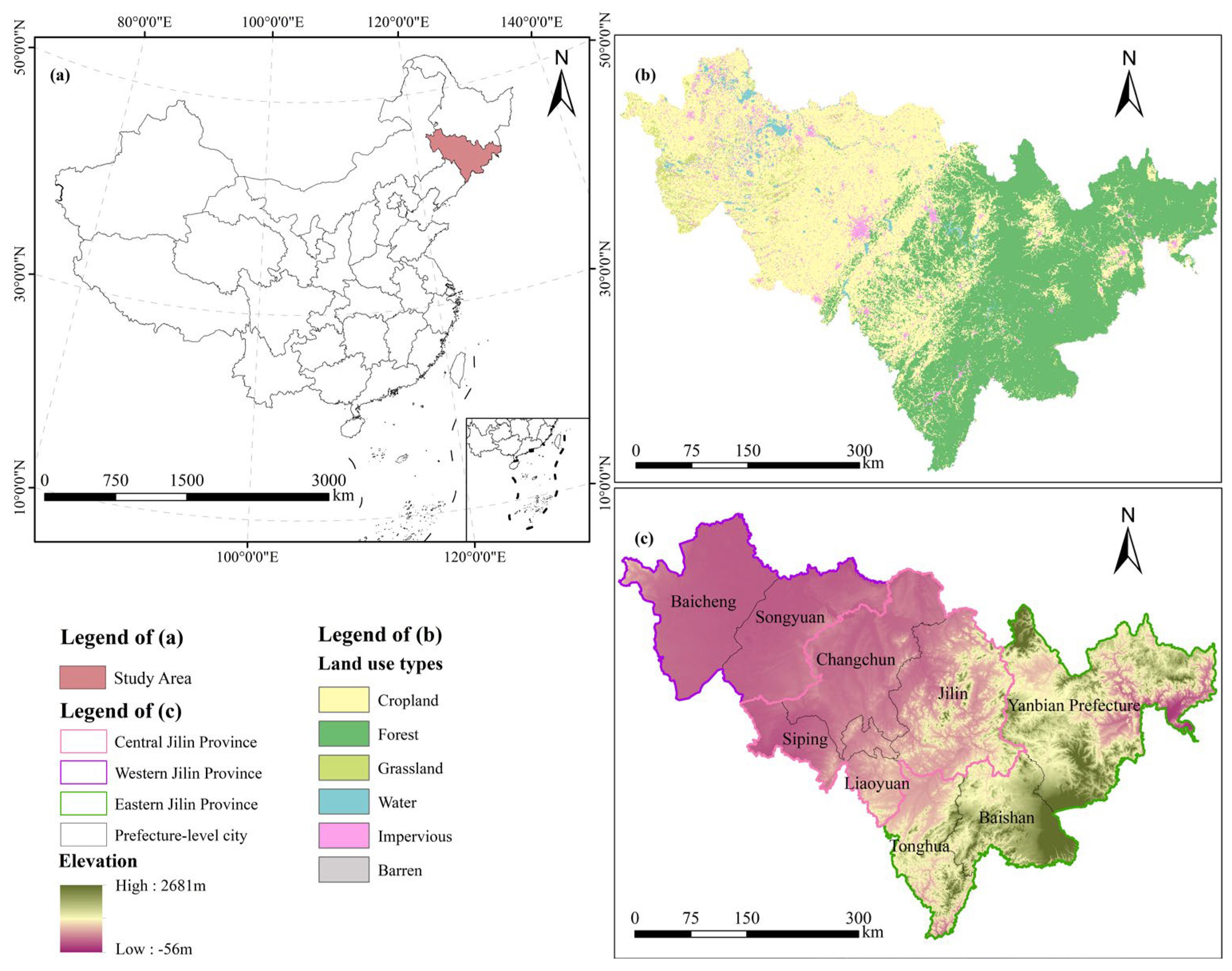
Situated in the central region of Northeast China and the geographical core of Northeast Asia, Jilin Province spans from 121°38′ to 131°19′E and 40°50′ to 46°19′N. Covering a total area of 187,400 km2, the region exhibits a distinct elevation gradient, sloping from higher elevations in the southeast to lower elevations in the northwest. This gradient delineates three primary geomorphic zones: the eastern mountains and hills, the central alluvial plains, and the western grasslands and wetlands (Figure 1).
As a vital national grain-producing base, Jilin Province plays a strategic role in safeguarding China’s food security. The province possesses extensive cropland endowed with fertile black soil and is globally recognized as lying within the Golden Corn Belt and Golden Rice Belt, with annual grain production consistently exceeding 40 million tons. Spatially, agricultural utilization exhibits significant heterogeneity. The flat and fertile central Songnen Plain serves as the primary area of high-quality, contiguous cropland, acting as the core zone for modern agriculture and large-scale operations. Conversely, the eastern Changbai Mountain region features complex topography and steep slopes, resulting in highly scattered cropland distribution. Meanwhile, the western region, situated within a farming-pastoral ecotone, has a fragile ecological environment where cropland is highly susceptible to wind erosion. This distinct spatial pattern of land utilization, shaped by the interplay of natural conditions and human activities, makes Jilin Province an ideal case study for investigating the nexus between cropland fragmentation and both production and ecological functions.

2.2. Data Sources

The data sources are listed in Table 1. Using ArcGIS 10.8 software, global and national datasets were projected and clipped to extract those specific to Jilin Province, producing data with a precision of 1000 m.

2.3. Methods

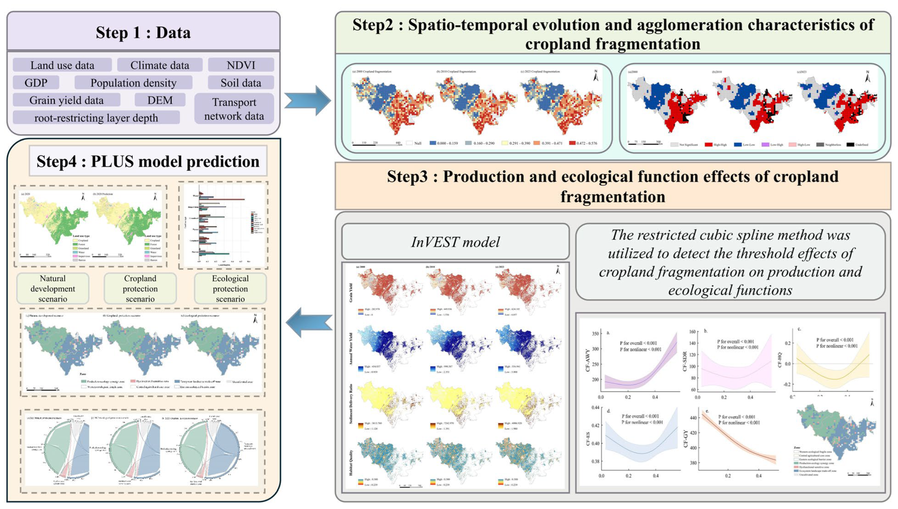
Building upon the analysis of the spatiotemporal dynamics and spatial clustering characteristics of cropland fragmentation in Jilin Province, this study quantifies its nonlinear effects on production and ecological functions. To accurately project future landscape configurations, the PLUS model is employed to simulate multiple land-use scenarios for 2030. Furthermore, informed by these nonlinear relationships, spatial zoning is delineated, and targeted regulatory strategies are proposed (Figure 2).

2.3.1. Quantitative Evaluation of Cropland Fragmentation

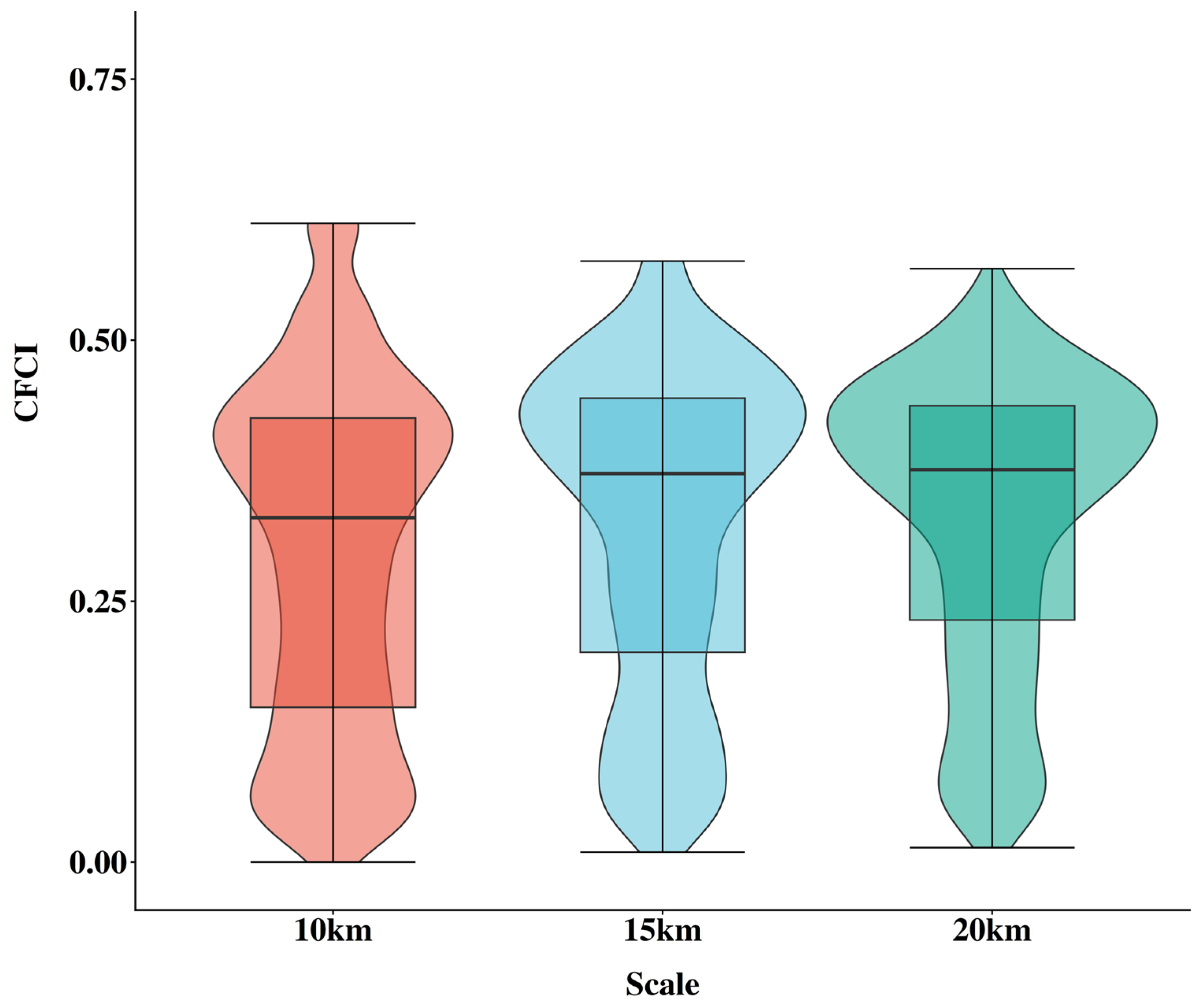
Regarding the analytical unit, provincial-scale fragmentation research typically employs grid scales ranging from 10 km to 20 km [42,43]. In this study, multi-scale sensitivity tests were conducted (Table A1, Figure A1 and Figure A2). The results indicated that at a 10 km scale, several grid units yielded a composite fragmentation index of zero, demonstrating an inability to effectively differentiate gradient variations within low-fragmentation areas. Conversely, a 20 km grid proved excessively coarse, risking the obscuration of localized landscape heterogeneity. Consequently, a 15 km grid was selected as the optimal analytical scale. The cropland landscape pattern indices within each grid were calculated, and the CRITIC method was used for weight assignment.
  • Indicator selection
(1)
NP (Number of Patches) serves as a direct indicator for landscape fragmentation levels, with higher values implying greater patch dispersion and increased fragmentation.
N P = N
N denotes the total count of patches belonging to a specific landscape category within the research region.
(2)
PD (Patch Density) quantifies the density of cropland patches per unit area; higher values indicate a greater degree of segmentation and more severe fragmentation.
P D = N A × 10,000 × 100
N represents the total patch count, while A stands for the total area of the study region (unit: m2).
(3)
AWMSI (Area-Weighted Mean Shape Index): When A W M S I equals 1, all patches are square; larger values indicate more irregular patch shapes.
A W M S I = i = 1 n 0.25 P i A i × A i i = 1 n A i
P i denotes the perimeter for patch i ;   A i represents the area for patch i ; and n is the total patch number.
(4)
SPLIT (Splitting Index) reflects the degree of spatial separation; larger values indicate more dispersed patch distribution and poorer landscape connectivity. When the landscape consists of a single patch, S P L I T = 1
S P L I T = A 2 i = 1 n A i 2
A is the total area of the study region; A i is the area of the i -th patch.
(5)
ED (Edge Density) indicates the total edge length normalized by unit area; larger values indicate more frequent exchanges of matter and energy between the landscape and external environments, and higher fragmentation.
E D = i = 1 n P i A × 10,000
P i refers to the perimeter of the i-th patch; A signifies the total landscape area (unit: m2).
(6)
AREA_MN (Mean Patch Area) indicates the average size of patches; lower values typically signal more severe fragmentation.
A R E A _ M N = i = 1 n A i N
A i is the area of the i -th patch; N represents the total quantity of patches.
(7)
COHESION (Patch Cohesion Index) evaluates landscape connectivity on a scale from 0 to 100. Higher scores suggest superior connectivity and reduced fragmentation.
C O H E S I O N = 1 i = 1 n P i i = 1 n P i A i × 1 1 Z 1 × 100
P i denotes the perimeter of patch i ; A i is the patch area; and Z corresponds to the total grid count in the study zone.
The constructed indicator system and weight assignments are shown in Table 2.
2.
Empowerment approach
The CRITIC method, first proposed by Diakoulaki et al. [44], utilizes the objective attributes of indicator data, considering the variability of indices, and measures correlations based on contrast intensity and indicator conflict to determine objective weights. The steps used to calculate it are as follows:
Step 1: Calculation of weight coefficients. Utilizing the results derived from the preceding steps, the specific weight coefficient for every individual indicator is calculated as follows:
P i j = X i j X imin / X imax X imin   Positive   Standardization Y imax Y i j / Y imax Y imin   Negative   Standardization
where P i j is the normalized dimensionless data, and X i j and Y i j are the landscape pattern metrics requiring forward or reverse standardization. Simultaneously, X i m i n and Y i m i n represent the lowest figures following forward or reverse normalization, and X imax and Y imax are the corresponding maximum values.
Step 2: Calculation of correlation coefficients. The product-moment variance method is applied to compute the interrelationship coefficients between the evaluation indicators.
r i j = m i j m i j P i j P i j m i j m i j 2 P i j P i j 2
In this equation, r i j represents the correlation coefficient, and m i j takes values X i j or Y i j . Additionally, m i j and P i j refer to the respective means.
Step 3: Determination of indicator conflict. The variability of the evaluation indicators is characterized using the standard deviation σ i .
C i = σ i j = 1 n 1 r i j
The variable n represents the total count of indicators sharing identical characteristics.
Step 4: Determination of weight coefficients. Based on the calculations from the previous steps, the weight coefficient for each indicator is finally determined.
W i = C i / j = 1 n C i
In Equation (11), W i represents the specific weighting factor assigned to the i-th indicator.
3.
Comprehensive calculation
To quantify the extent of cropland fragmentation, a composite index (CFCI) was calculated for every grid unit using the equation presented below:
C F C I = i = 1 m P i j W i
In the equation above, CFCI refers to the composite index measuring cultivated land fragmentation; Pij stands for the standardized value corresponding to the i-th index, while Wi signifies the weight allocated to that specific index.

2.3.2. Spatial Autocorrelation Analysis of Cropland Fragmentation

This study utilizes spatial autocorrelation analysis [45,46,47], incorporating both global and local spatial autocorrelation evaluations [48,49]. The Global Moran’s I index is utilized to quantify the overall spatial distribution characteristics, with values ranging from −1 to 1, indicating the degree of spatial aggregation or dispersion across the study area. Subsequently, Local Moran’s I is applied to identify localized spatial clusters and outliers. The spatial clustering patterns and interactions between grid units are visualized through LISA maps [50]. Spatial analysis was conducted using GeoDa 1.22. The formulas used next are outlined below:
Global   Moran s I = i n j i n w i j x i x ¯ x j x ¯ S 2 i n j i n w i j
Local   Moran s I = x i x ¯ S 2 j i n w i j x j x ¯
S 2 = 1 n i n x i x ¯ 2
x ¯ = 1 n i n x i
where n is the number of patches within the study area, xi and xj are the comprehensive indices of cropland fragmentation for the i-th and j-th patches, respectively; wij is the spatial weight matrix, and S2 and x ¯ are the variance and mean of the comprehensive indices of cropland fragmentation for all patches in the study area, respectively.

2.3.3. Quantitative Evaluation of the Relationship Between Cropland Production and Ecological Functions with Cropland Fragmentation

  • Evaluation of production and ecological functions
(1)
Production function evaluation
NDVI is adopted as a proxy for grain yield estimation. NDVI serves as a robust metric of vegetation vigor and exhibits a significant positive correlation with crop yield, a relationship with demonstrated applicability across diverse crop types and geographical regions [51,52,53,54]. Furthermore, this correlation has been rigorously validated within the black soil region of Northeast China [55,56]. Although this approach does not explicitly disaggregate the effects of crop type, management intensity, or soil fertility, NDVI integrates these factors through canopy response, and in Jilin Province’s relatively homogeneous cropping system, this approach preserves the spatial rank structure of grain productivity that underpins the RCS threshold analysis. The formula is expressed as follows:
G Y i = G s u m × N D V I i N D V I s u m
where G Y i is the grain production of cropland grid i (t/km2); G s u m is the total grain production of the study area (t); N D V I i is the normalized difference vegetation index of the i-th cropland grid; N D V I s u m is the sum of the normalized vegetation index for cropland in the study area.
(2)
Ecological function evaluation
InVEST empowers us to evaluate quantifiable trade-offs regarding alternative management strategies [57,58]. It also pinpoints locations where natural capital investment fosters human development alongside conservation [59]. This study selects annual water yield, sediment delivery ratio, and habitat quality for ecological function evaluation in the study area (Table A2 and Table A3).
  • Annual water yield
Annual water yield is an important water supply service. The specific formula for calculating it is
Y ( x ) = 1 A E T ( X ) P ( X ) P ( x )
where Y ( x ) is the annual water yield of the grid; P ( X ) is the annual precipitation of the grid; and A E T ( X ) is the annual actual evapotranspiration of the grid.
b.
Sediment delivery ratio
The sediment delivery ratio regulates the reduction in soil erosion caused by water erosion. The specific formula for calculating it is
S C i S = R K L S U S L E = R × K × L S × 1 C × P
where S C i S refers to the amount of soil retention ( t h m 2 a 1 ), RKLS indicates the amount of potential soil erosion ( t h m 2 a 1 ), and USLE represents the amount of actual soil erosion ( t h m 2 a 1 ). The basic data required includes the rainfall erosivity factor R, soil erodibility factor K, vegetation cover and crop management factor C, soil conservation practice factor P, and topographic slope factor LS.
c.
Habitat quality
The specific formula for calculating habitat quality is
Q x j = H j ( 1 D x j z D x j z + K z )
Q x j = r = 1 R   y = 1 Y r   W r   r = 1 R   W r r y i r x y β x S j r
In these equations, Qxj represents the habitat quality for grid x within land use type j, while Dxj denotes the total threat level. K and Z are scaling constants, and Hj refers to the habitat suitability of land use type j. R identifies the stress factor, with Yr indicating the number of grids occupied by this factor. The weight assigned to the threat factor (ranging from 0 to 1) is given by Wr. Additionally, ry is the stress value for grid y, and irxy quantifies the impact of this stress from grid y on grid x. Finally, βx represents the accessibility of grid x, and Sjr defines the sensitivity of the habitat type to the specific stress factor.
2.
Correlation relationship
The restricted cubic spline (RCS) is a nonlinear fitting method often used for modeling smooth nonlinear relationships between independent and dependent variables [60].
The RCS also offers additional advantages in realization and interpretation [61]. The transformation with k knots replaces the original covariate x with k-1 new variables, and the initial variable among the newly generated ones invariably corresponds to the original covariate x. For example, a logistic regression model that includes an RCS transformation of x has the following form:
l o g odds = β 0 + β 1 s p 1 ( x ) + β 2 s p 2 ( x )
where s p 1 ( x ) is the original covariate x , and s p 2 ( x ) is a complex function of the original variable and the knot locations.

2.3.4. Scenario Simulation and Prediction of Cropland Fragmentation Patterns

The PLUS model [62] is a grid-based cellular automata (CA) model suitable for simulating patch-scale land use change.
Randomly extracting expansion areas of land use types in two periods as training samples, combined with a random forest algorithm, explores the relationship between land use type expansion and driving factors.
The CARS model is a scenario-driven simulation framework that primarily predicts regional land use distribution patterns by constraining the development probability of various land use types. Driving factors incorporate natural, accessibility, and socio-economic dimensions, following established practice in CA-based land-use simulation [63]. Parameter values follow the developer’s recommended defaults and recent applications [64,65,66].

3. Results

3.1. Temporal and Spatial Evolution of Cropland Fragmentation

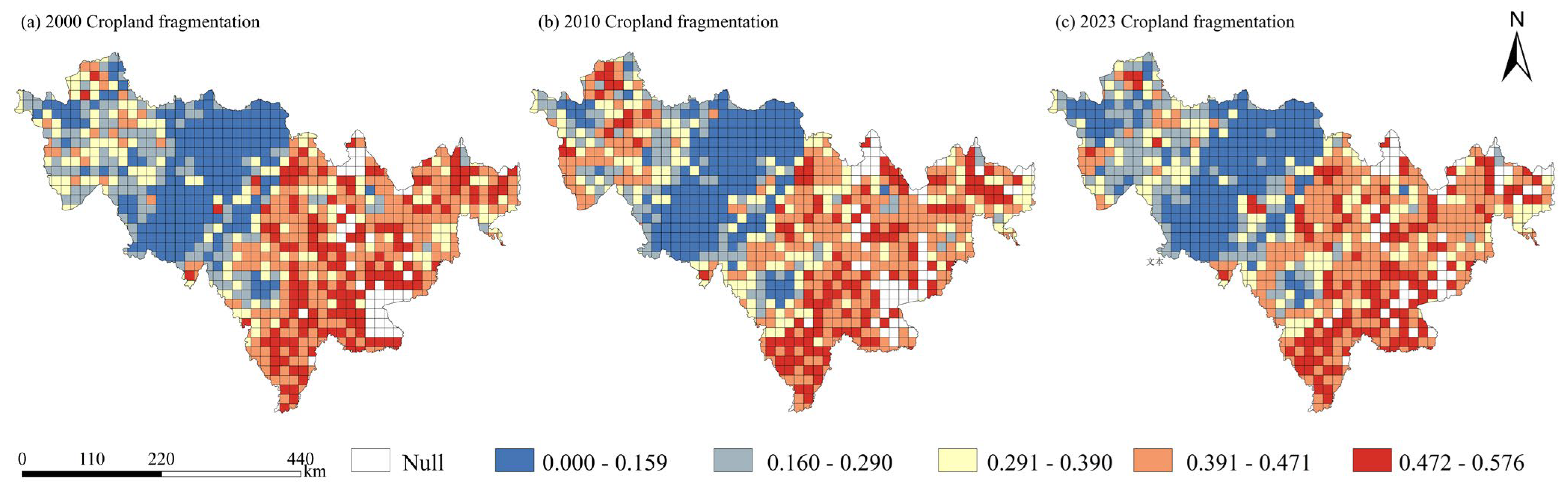
The comprehensive indices of cropland fragmentation for the years 2000, 2010, and 2023 in the study area are shown in Figure 3. From a temporal perspective, the mean Cropland Fragmentation Composite Index (CFCI) in Jilin Province increased from 0.321 in 2000 to 0.331 in 2010, representing an increase of approximately 3.1%. This trend reflects the intensification of fragmentation driven by rapid urbanization and infrastructure expansion. However, from 2010 to 2023, the mean CFCI declined to 0.324, a 2.1% reduction relative to 2010. This reversal suggests that high-standard farmland construction and land consolidation initiatives have effectively mitigated localized fragmentation. In terms of spatial differentiation, the relative regional patterns remained largely stable over the past two decades, although the intensity of fluctuations varied significantly across regions. The central Songnen Plain consistently maintained a low-fragmentation state with minimal fluctuations, benefiting from inherently contiguous cropland and high levels of agricultural mechanization. Conversely, the eastern mountainous regions, constrained by rugged topography and naturally dispersed parcels, have long exhibited persistent high fragmentation with limited mitigation. The western ecologically vulnerable zones demonstrated pronounced temporal volatility, particularly in the Baicheng region, where intense transitions underscore the dual sensitivity of land use to both policy-driven adjustments and natural environmental fluctuations. In summary, the spatiotemporal trajectory of cropland fragmentation in Jilin Province is not a simple linear progression but a complex, nonlinear response to the synergistic interplay of biophysical constraints and phased anthropogenic interventions.

3.2. Spatial Aggregation Characteristics of Cropland Fragmentation

As shown in Table 3, cropland fragmentation presents significant spatial variation, identified through four relationship patterns: HH, LL, HL, and LH. The HH and LL types characterize spatial agglomeration, referring to clusters of similar values (high–high or low–low). Conversely, HL and LH denote spatial outliers, describing specific areas where high values are surrounded by low values (HL) or low values by high values (LH).
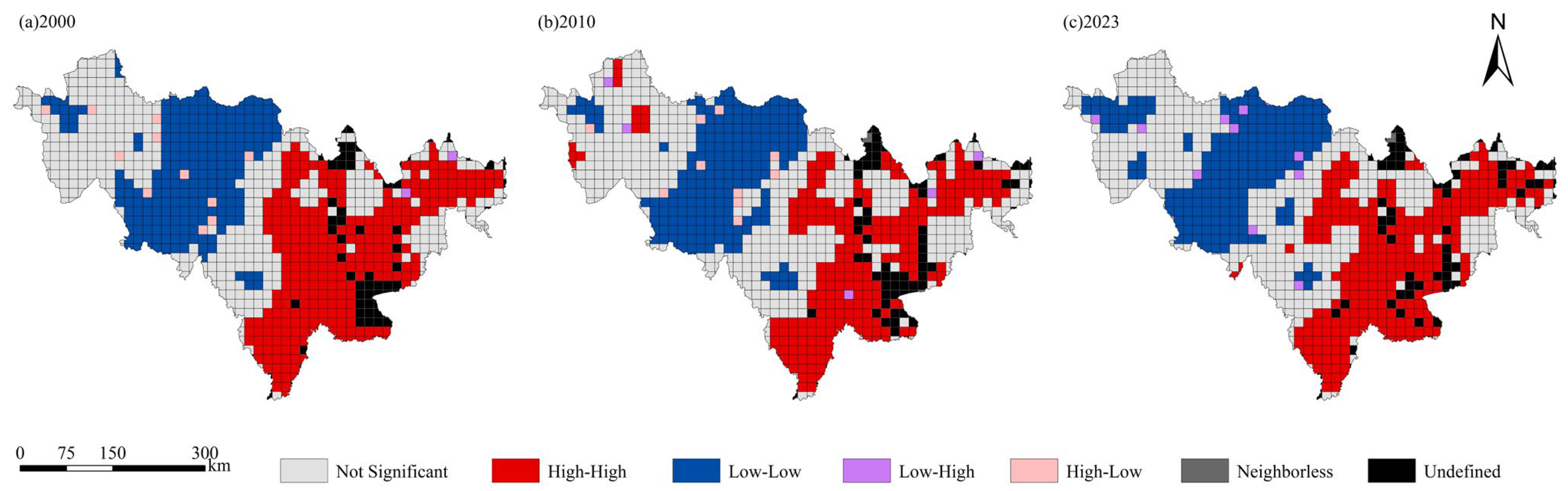
Spatial autocorrelation analysis reveals that cropland fragmentation in Jilin Province exhibits significant spatial heterogeneity and pronounced clustering characteristics. Spatially, a distinct structural pattern emerged: elevated fragmentation in the east, contiguous cropland in the central core, and mixed spatial associations in the west (Figure 4). The HH spatial clusters were primarily concentrated in the eastern mountainous regions, exhibiting an initial spatial contraction followed by subsequent expansion throughout the study period. Conversely, the central region maintained stable LL clusters, constituting a persistent cold spot of fragmentation. The spatial clustering pattern in the western region experienced continuous restructuring, transitioning from a predominantly LL pattern with scattered HL clusters, through a mix of HH and LL, to the current coexistence of LL and LH clusters. This spatial restructuring was driven by the shifting dominance of anthropogenic and ecological drivers across different stages. In the early stage, traditional farming dominated, resulting in generally low fragmentation and stable LL clusters interspersed with isolated HL outliers. Subsequently, ecological conversion programs, such as returning cropland to forest and grassland, and infrastructure expansion exacerbated local fragmentation, generating HH clusters. In the later stage, while sustained land consolidation facilitated the recovery of low-fragmentation patches (LL), intensifying urbanization pressures forged an LH pattern, wherein contiguous cropland became spatially constrained by highly fragmented surroundings.
Moreover, HL and LH spatial outliers were relatively dispersed across the province. The gradual transition of HL clusters to LH clusters further underscores the intensifying pressure and spatial restructuring of cropland driven by urbanization.

3.3. Production and Ecological Function Effects of Cropland Fragmentation

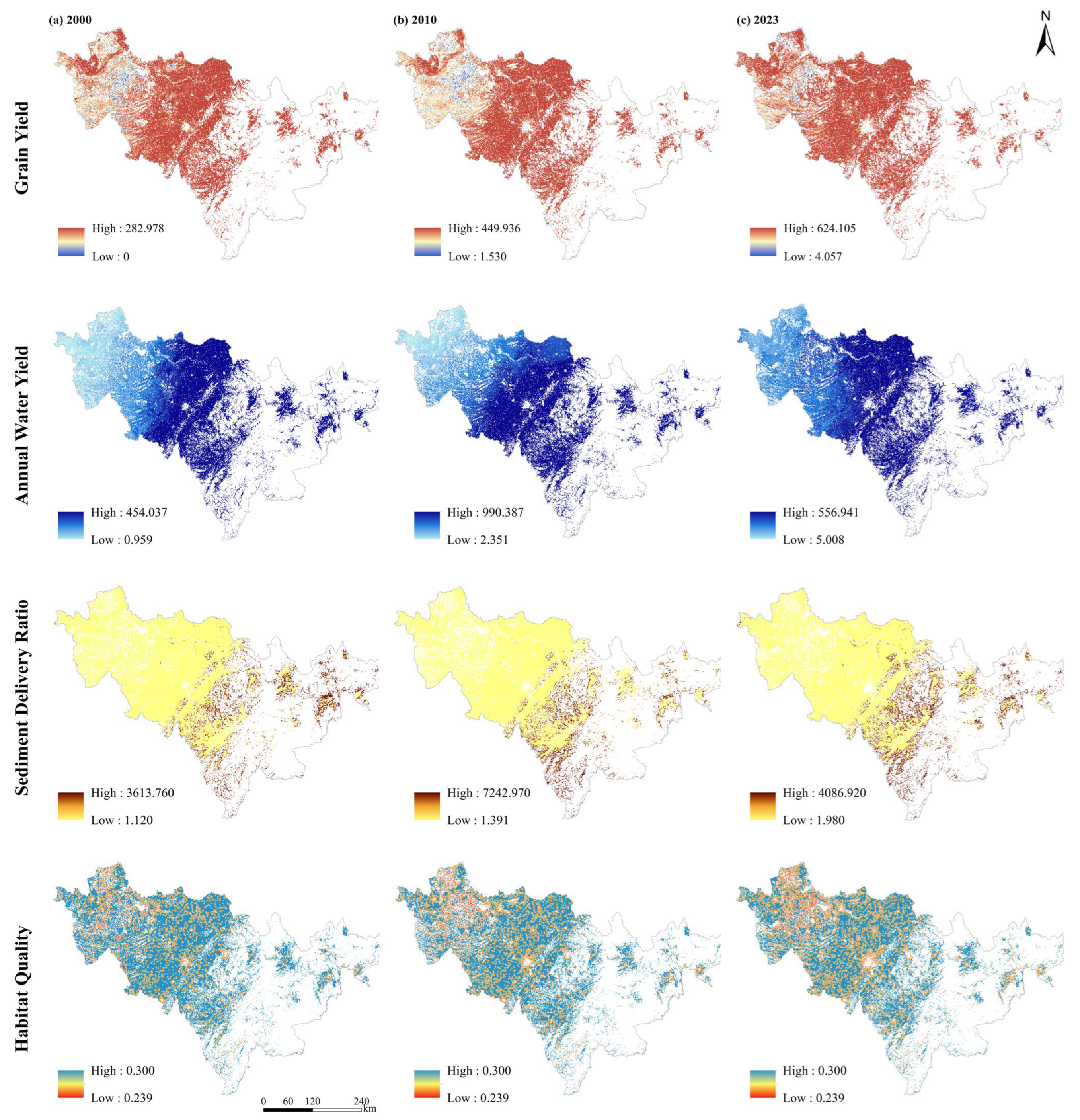
Following the quantification of production and ecological functions from 2000 to 2023, cropland extents were extracted using a spatial mask to specifically analyze their correlation with fragmentation (Figure 5). Temporally, grain yield exhibited a continuous upward trajectory, surging by 219.12% over the study period. Regional precipitation, a key ecological proxy, demonstrated an inverted U-shaped trend, with the spatial center of peak values migrating from Yanbian Prefecture in the east to Liaoyuan City in the south-central region. Soil retention capacity remained generally low, with elevated values exhibiting a dispersed pattern, primarily concentrated within Jilin and Tonghua cities. Habitat quality manifested a highly interspersed spatial mosaic. High-value patches were predominantly concentrated in the central region, whereas the western region experienced degradation. Concurrently, the spatial extent of low-value zones progressively expanded, while habitat quality in the eastern region remained relatively stable.
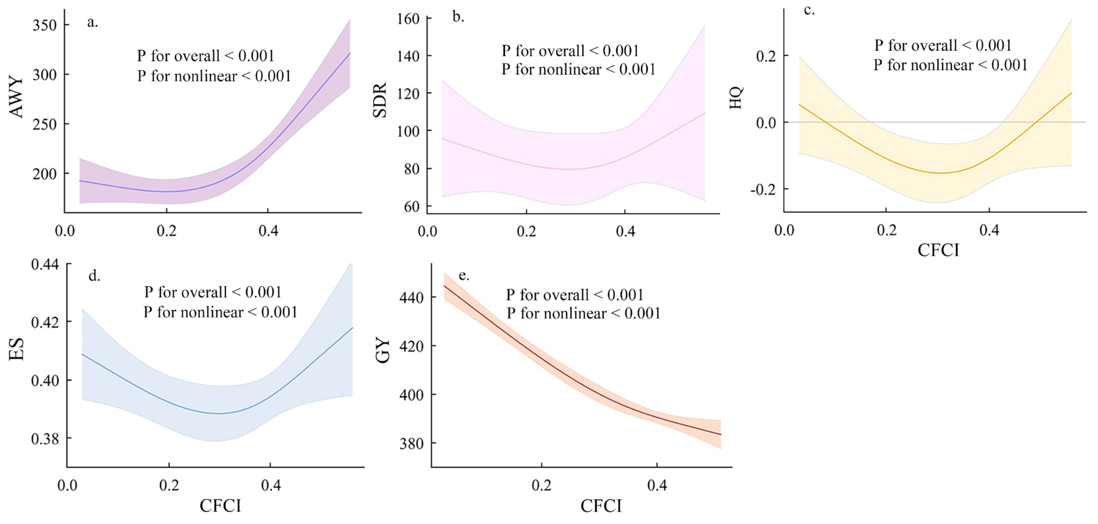
RCS models (Table 4) were employed to quantitatively evaluate the relationship between the CFCI and both production and ecological functions. This approach enables the precise identification of critical inflection points, clarifying the thresholds at which fragmentation triggers directional shifts in functional performance. Due to insufficient variability in the original data on habitat quality, a Z-score standardization was applied.
The RCS results indicate highly significant nonlinear relationships between cropland fragmentation and both production and ecological functions. The overall significance of all constructed models, as well as the significance of the nonlinear terms, was highly robust (p < 0.001). These findings provide statistical evidence for the complex, threshold-dependent interaction mechanisms through which spatial fragmentation governs the multifunctionality of cropland.
Specifically (Figure 6), grain yield exhibits a continuous decline with intensifying fragmentation and shows no evident rebound. This highlights the persistent negative impact of spatial fragmentation on agricultural output, indicating that maintaining contiguous cropland and large-scale operations remains pivotal for ensuring food security. Conversely, ecological indicators, including annual water yield, sediment delivery ratio, and habitat quality, all exhibit a distinct U-shaped response. These ecological functions deteriorate initially, reaching a nadir at a critical CFCI threshold of 0.363, beyond which they gradually recover as fragmentation further intensifies. Mechanistically, during the intermediate stages of fragmentation, habitat loss and the disruption of ecological corridors lead to the nadir of ecological performance. However, as fragmentation becomes severe, it often triggers the implementation of ecological engineering and restoration programs, such as afforestation and grassland recovery, in highly fragmented regions, which significantly enhance water retention and soil conservation capabilities. Furthermore, the increased structural complexity in these highly fragmented landscapes can elevate surface roughness, thereby decelerating surface runoff. Consequently, the overarching U-shaped trajectory of the ecosystem emerges from these complex socio-ecological trade-offs.
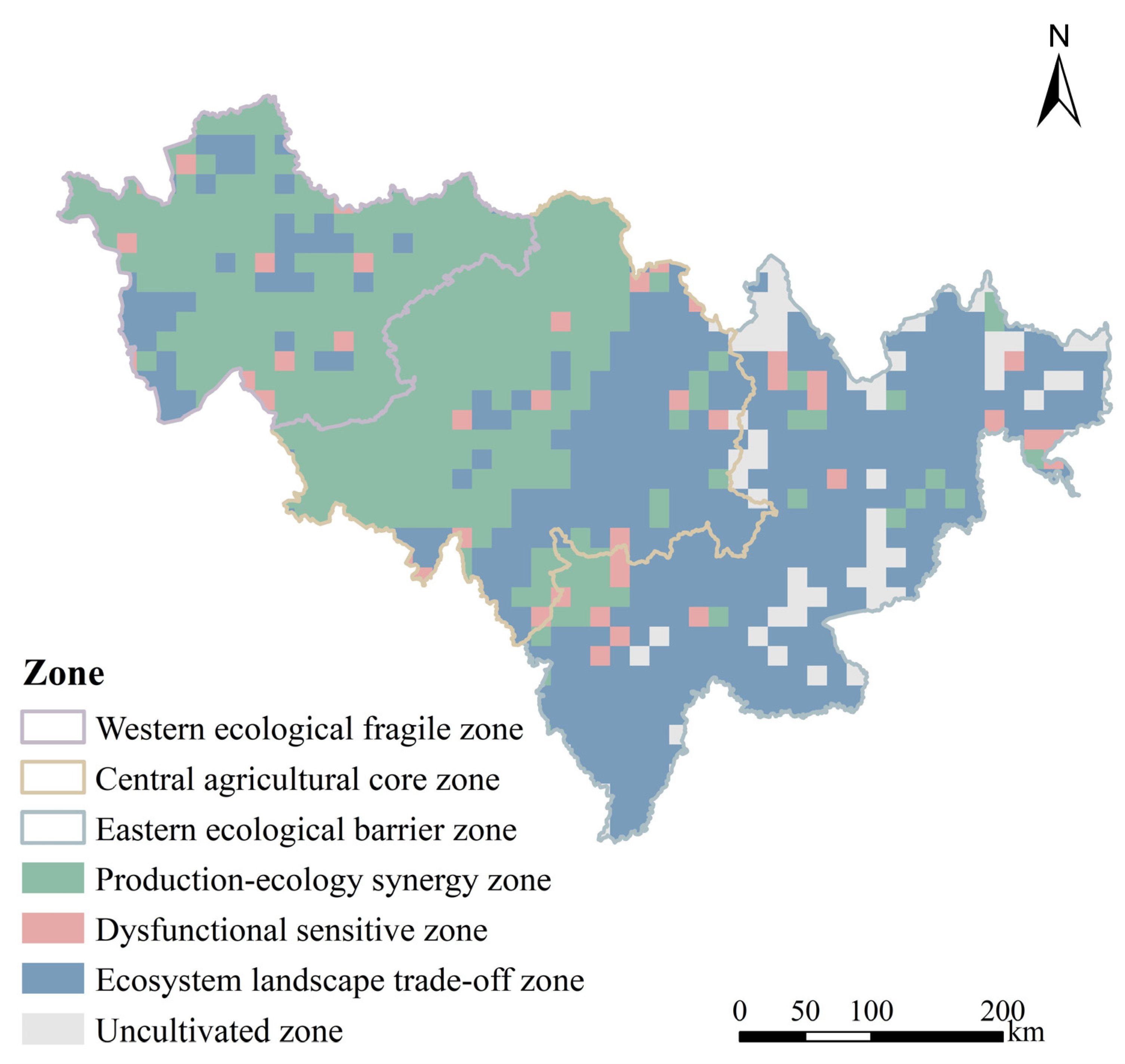
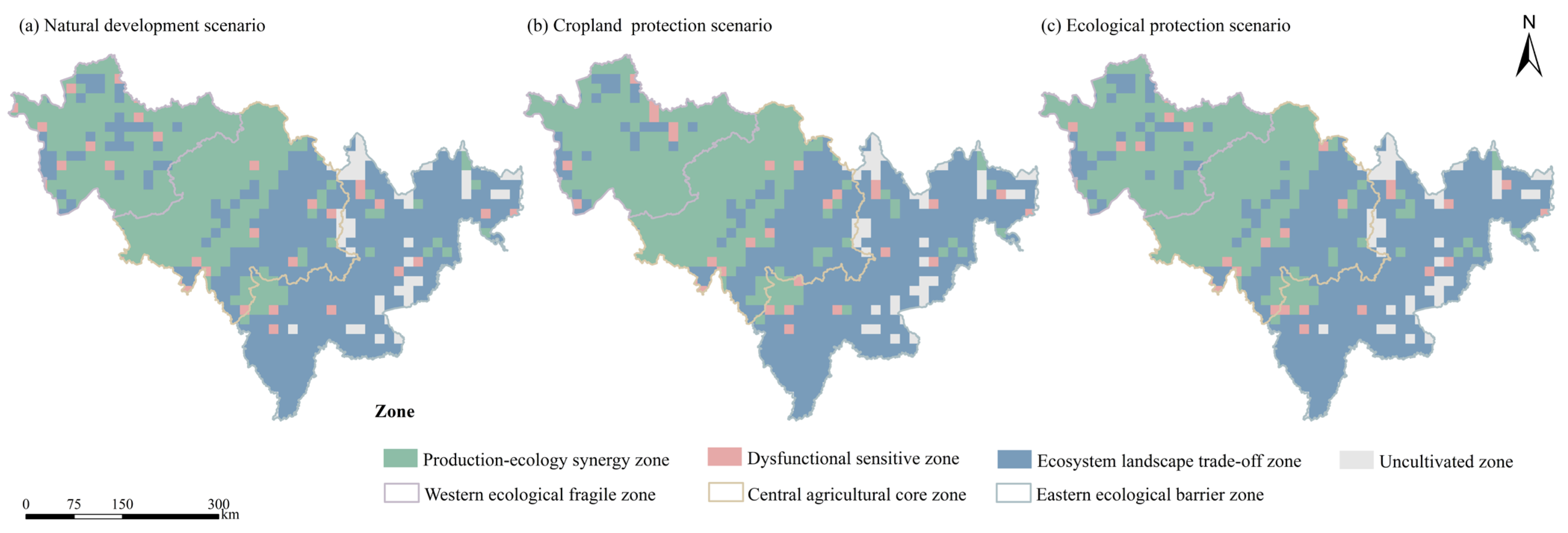
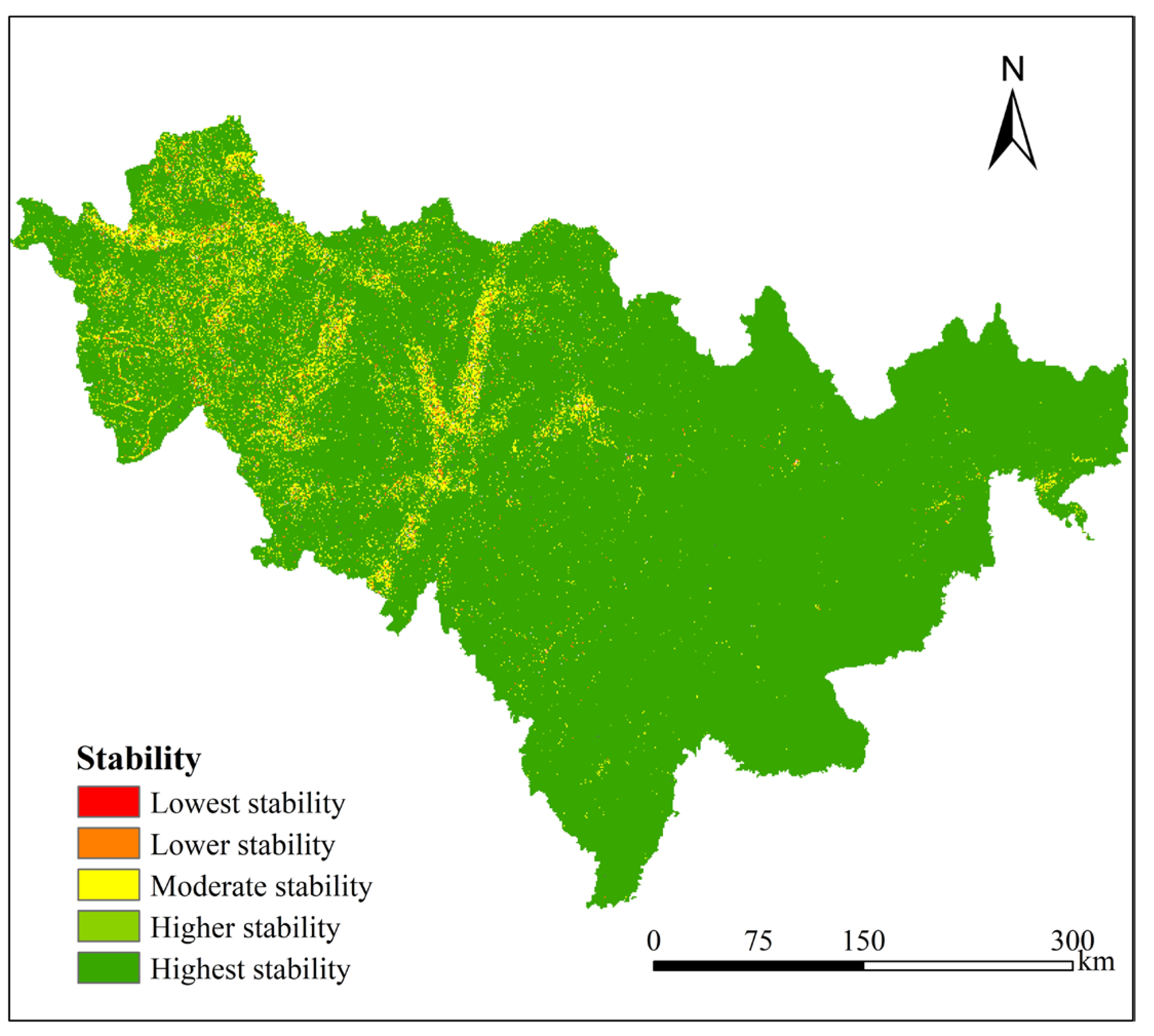
Based on the identified nonlinear thresholds, the spatial domain is delineated into three distinct regulatory typologies (Figure 7): Production–ecology Synergy Zones (CFCI < 0.340), dysfunctional sensitive zones (0.340 ≤ CFCI ≤ 0.363), and ecosystem landscape trade-off zones (CFCI > 0.363). The central plain region is overwhelmingly dominated by production–ecology synergy zones, with dysfunctional sensitive zones appearing only sporadically. Ecosystem landscape trade-off zones are patchily embedded within the low mountains and hills along the southeastern periphery. The robust synergy between production and ecological functions in this area establishes it as an optimal agricultural stabilization zone. In the western ecologically fragile region, all three functional typologies coexist, with dysfunctional sensitive zones constituting a more substantial proportion than in the central and eastern regions. Here, synergy zones are constrained to tracts of highly contiguous cropland, whereas trade-off zones are concentrated adjacent to wetlands and aquatic bodies. The intricate spatial interweaving and transitional boundaries among these zones suggest that the regional ecological carrying capacity is approaching critical tipping points, rendering its functional equilibrium highly sensitive to fragmentation disturbances. The eastern mountainous region is predominantly occupied by ecosystem landscape trade-off zones. Owing to severe topographic constraints, large-scale contiguous cultivation is precluded. Consequently, production–ecology synergy zones are highly fragmented, and dysfunctional sensitive zones manifest merely as isolated enclaves.

3.4. Prediction of Future Patterns of Cropland Fragmentation

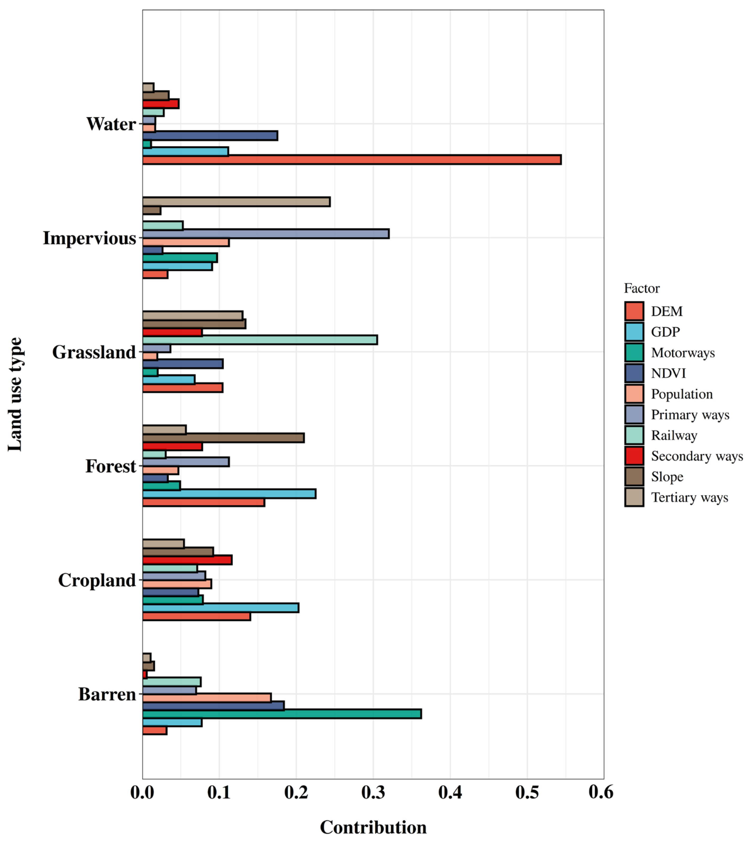
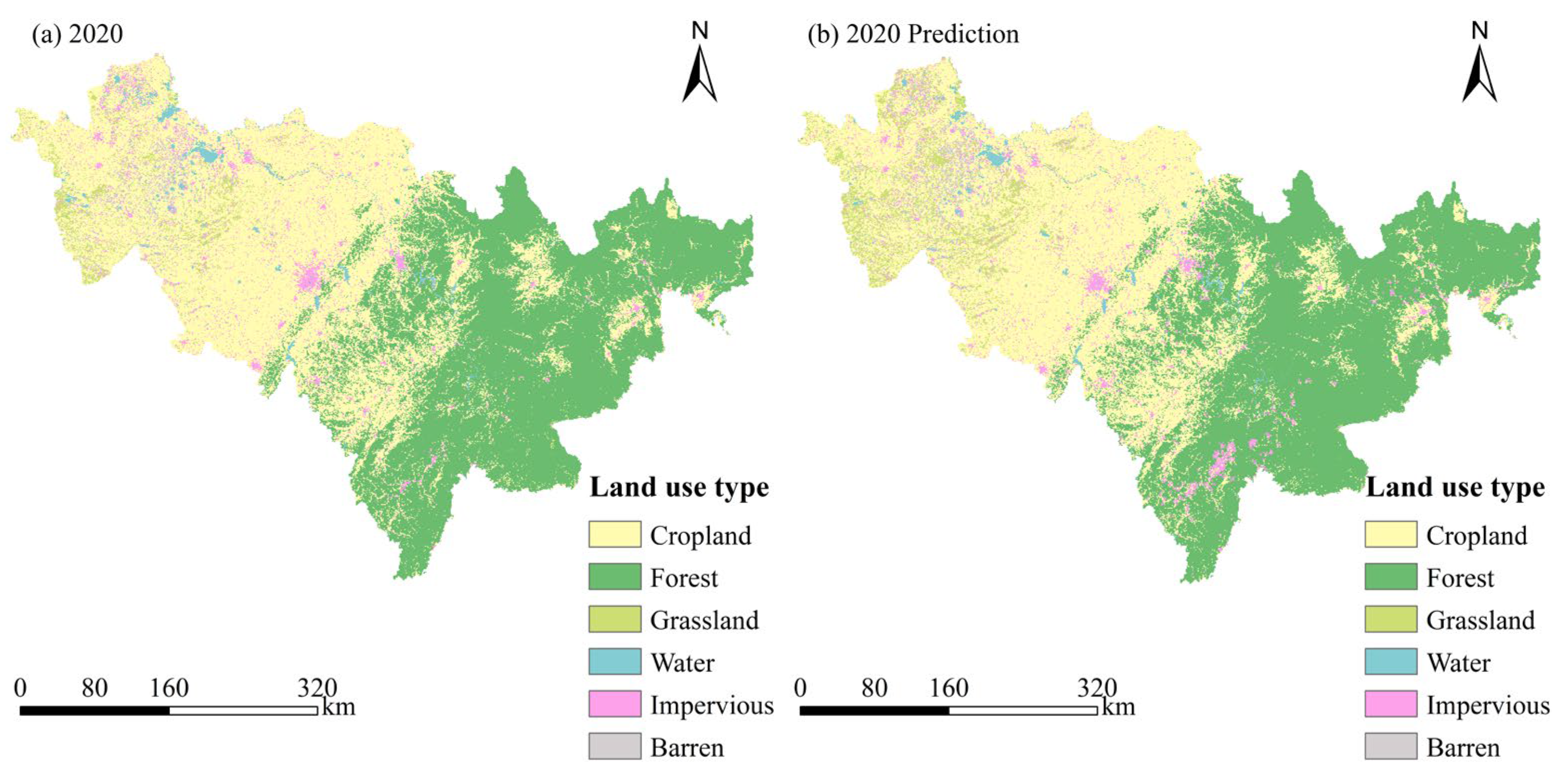
Using the PLUS model and historical data from 2000, 2010, and 2020, multi-scenario land-use configurations for Jilin Province were projected for 2030 (Table A4, Table A5 and Table A6). The LEAS module quantified the contribution of ten driving factors to land-use expansion (Figure 8). Socioeconomic and infrastructural factors predominantly drove the expansion of impervious surfaces and barren land, with major roads and highways as the leading contributors, underscoring the critical role of transport accessibility in urban growth. Grassland expansion was driven primarily by railway proximity, likely reflecting vegetation restoration or specific land utilization along rail corridors. Conversely, water body distribution was strictly constrained by DEM, reflecting the strong topographic control over hydrological features. Furthermore, GDP exerted a widespread driving force on both cropland and forest dynamics, highlighting the pervasive influence of economic development in shaping coupled patterns of production and ecology. Model validation yielded a Kappa coefficient of 0.861, an overall accuracy of 0.917, and a FoM of 0.102 (Figure 9). To further validate the results, the PLUS model was run 20 times, and the standard deviation and coefficient of variation were calculated, followed by a stability test (Table A7 and Figure A3). The FoM value is consistent with typical results reported for provincial-scale CA simulations over decadal horizons, where the proportion of actual change is small and mathematically bounds the achievable FoM [67]. The high Kappa (0.861) and overall accuracy (0.917), together with the aggregate-level stability of scenario outputs, support the reliability of the scenario-based zoning conclusions.
Guided by relevant regional policies and Jilin Province’s future strategic positioning, three distinct simulation pathways were established: the natural development scenario (NDS), the cropland protection scenario (CPS), and the ecological protection scenario (EPS) [68].
Spatial projections for 2030 (Figure 10) reveal that under the NDS, the spatial extent of dysfunctional sensitive zones within the western ecologically fragile region exhibits a pronounced expansion. This confirms the inherent vulnerability of this region, which remains precariously situated at the nadir of the ecological U-shaped curve. The CPS focuses on stabilizing the central agricultural core, aiming to keep fragmentation below the 0.340 threshold, thereby maintaining grain yields at their optimal levels; however, it correspondingly allocates insufficient attention to the high-value ecological zones in the east. The EPS, conversely, expands the ecosystem landscape trade-off zones, aligning with the mechanism that extreme fragmentation in the eastern mountainous areas corresponds to elevated ecological performance, the ascending branch of the U-shaped curve, thereby achieving an overall ecological enhancement through the prioritization of ecological land. Notably, the EPS framework does not enforce rigid restrictive boundaries on Permanent Basic Cropland. Consequently, these simulated results represent theoretical ecological potential; in practice, the actual scale of land conversion will be strictly regulated by definitive policy pathways.
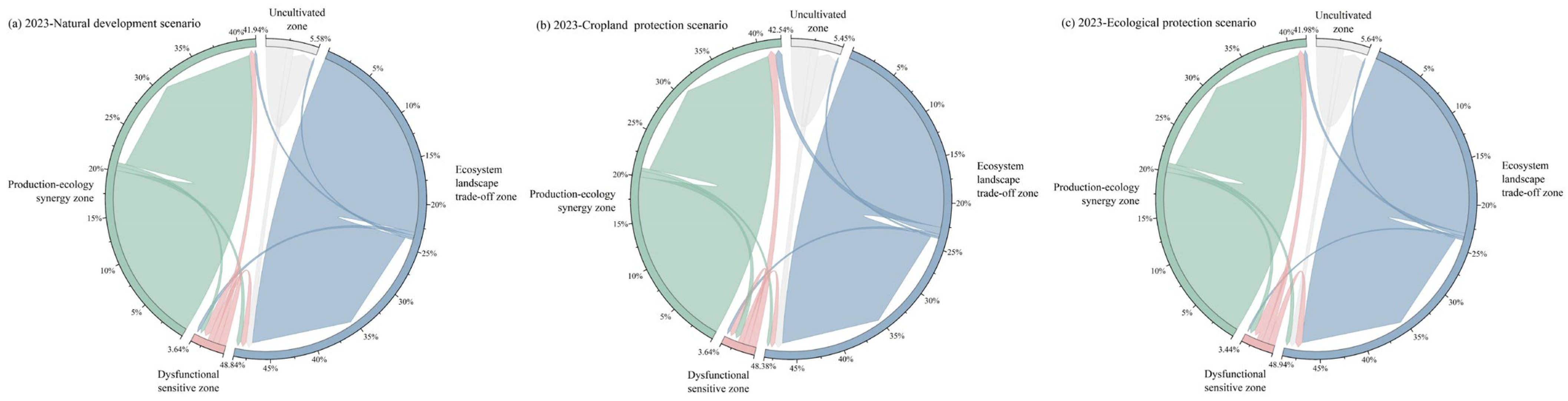
Based on the chord diagram analysis (Figure 11), the three scenarios exhibit markedly divergent transitional trajectories (Table A8). Under the NDS, 1536.78 km2 of production–ecology synergy zones devolve into dysfunctional sensitive zones, exposing the risk of unregulated, latent ecological degradation. The CPS facilitates the transition of 3359.62 km2 from sensitive zones back to synergy zones, effectively reinforcing production functions on the left side of the U-shaped curve. However, this singular policy focus concurrently triggers a reciprocal degradation of 2518.66 km2 within the synergy zones, thereby introducing systemic stability risks. In contrast, the EPS successfully drives the conversion of 2821.04 km2 from sensitive zones into ecosystem landscape trade-off zones and sustains the highest stable stock of trade-off zones at 88,352.39 km2. This trajectory effectively steers the western fragile region across the functional nadir, transitioning it toward an ecologically optimized state on the right side of the functional curve.

4. Discussion

4.1. The Nonlinear Relationship Between Cropland Fragmentation and Production and Ecological Functions

The relationship between grain yield and cropland fragmentation is distinctly nonlinear, characterized by an attenuating marginal negative effect beyond a critical threshold of 0.340. Approaching this threshold from the lower end, fragmentation exerts a severe negative impact on grain yield by drastically restricting the maneuverability of agricultural mechanization and inflating production costs [14]. However, once fragmentation exceeds this threshold, the decline in yield stabilizes. This plateau suggests the emergence of complex adaptive agricultural practices and localized resilience in response to severe spatial constraints.
Crucially, ecological services exhibit a consistent U-shaped response trajectory, with an inflection point at a threshold of 0.363. During the initial, low-fragmentation phase, landscape homogenization suppresses ecosystem resilience and diminishes biodiversity [69]. However, as fragmentation intensifies beyond the critical threshold, the integration of non-agricultural patches significantly increases landscape heterogeneity. The ecological corridors formed by these agroforestry mosaics effectively enhance habitat quality and soil retention capacity [70]. This finding provides robust empirical evidence that highly fragmented agricultural landscapes can, paradoxically, be leveraged to generate collateral ecological benefits.

4.2. Qualitative Analysis of Influencing Factors of Cropland Fragmentation Spatial Pattern

Although this study primarily focuses on quantifying the nonlinear impacts of cropland fragmentation on both production and ecological functions, elucidating the underlying driving mechanisms behind these spatial patterns in Jilin Province is essential for formulating targeted spatial interventions.
Physiographically, the undulating topography and dense forest coverage in the eastern mountainous regions constitute the primary natural drivers of the persistently high fragmentation observed there. In the ecologically fragile western region, severe risks of soil salinization and desertification, compounded by historical policy oscillations between unregulated agricultural expansion and ecological restoration, have generated highly volatile fragmentation dynamics. Socioeconomically, the central plain region, despite its flat terrain and inherently high parcel connectivity as a core grain-producing area, has experienced intense and rapid urbanization in recent years. Furthermore, under the household contract responsibility system, smallholders independently manage scattered plots, structurally sustaining physical fragmentation. The growing prevalence of part-time farming and rural out-migration further weakens farmers’ willingness to consolidate parcels, resulting in localized abandonment and de facto parcelization. Rising non-farm wages increase the opportunity cost of agricultural labor, discouraging investment in parcel consolidation. Where the land transfer market remains underdeveloped and transaction costs are high, fragmented holdings cannot be reconsolidated, crystallizing into the persistent spatial pattern captured in our analysis. Ultimately, the complex coupling of economic and institutional evolution, infrastructural expansion, and geomorphic constraints shapes the pronounced spatial heterogeneity of cropland fragmentation in Jilin Province. This multidimensional driving mechanism underscores the realistic imperative for implementing the differentiated zoning regulations proposed in this study.

4.3. Regulatory Recommendations for Different Regions

Based on the threshold identification and multi-scenario analyses, spatially differentiated regulatory strategies are proposed for Jilin Province. These recommendations aim to harmonize agricultural development with ecological preservation through site-specific land management paradigms.
Production–ecology synergy zones are predominantly located within the major grain-producing areas of the central Songnen Plain, where the CFCI remains generally below 0.340. The RCS analysis reveals a strong negative marginal effect of fragmentation on grain yield within this range, indicating that even minor increases in spatial fragmentation can induce a highly sensitive decline in agricultural output. Consequently, maintaining contiguous cropland in these central plains is of paramount policy importance for safeguarding grain production capacity. Spatial regulation must prioritize consolidation: continuously advancing high-standard cropland construction and comprehensive regional land consolidation can preserve and enhance parcel contiguity. Simultaneously, strictly regulating the conversion of high-quality cropland in territorial spatial planning is essential [71]. Multi-scenario simulations indicate that under the NDS, portions of these synergy zones devolve into dysfunctional sensitive zones, underscoring that without targeted spatial controls, the existing synergistic baseline may progressively erode.
Dysfunctional sensitive zones are concentrated in the ecologically fragile western region, corresponding to a CFCI range of 0.340 to 0.363. This transitional range faces compounding pressures: production capacity declines steadily with escalating fragmentation, while ecological functions remain trapped near the nadir of the U-shaped curve, signifying fundamentally compromised system resilience. The regulatory framework here should emphasize risk identification and typology-based restoration. For severely degraded marginal cropland, priority should be given to assessing the feasibility of reconversion to grassland or wetland ecosystems. For scattered patches retaining restorative potential, land consolidation should be employed to optimize spatial configurations, thereby facilitating functional recovery. Multi-scenario analyses reveal that while the CPS partially bolsters production functions, it fails to elevate these sensitive zones out of the ecological nadir, leaving systemic vulnerabilities intact. Conversely, the EPS successfully navigates certain sensitive areas into trade-off zones, elevating ecological functions beyond the critical threshold. This juxtaposition highlights that a singular policy focus is inadequate for resolving the complex trade-offs between production and ecology, whereas differentiated restoration rooted in regional classification offers superior adaptive capacity.
Ecosystem landscape trade-off zones primarily occupy the eastern mountainous areas, where fragmentation indices are elevated, locally exceeding 0.363. In these areas, comprehensive ecological functions have surpassed the U-curve nadir, exhibiting a resilient rebound as fragmentation increases. This dynamic is primarily attributable to the habitat diversity generated by structural landscape heterogeneity and the ecological corridor effects inherent to agroforestry ecotones. Under the framework of Permanent Basic Cropland protection, directly transplanting the large-scale contiguous consolidation paradigm of the central plains to this region is biologically and topographically inappropriate. Instead, policy interventions should prioritize maintaining the stability of the existing agroforestry mosaic, safeguarding established bio-corridors and critical habitat patches, and fostering diversified localized economies, such as under-story agroforestry and eco-agriculture, that align with overarching cropland protection mandates [72]. Simulations demonstrate that under the EPS, this zone remains one of the province’s most robust ecosystem service providers; preserving its current function as the principal spatial carrier of ecological land is a strategically prudent choice.

4.4. Limitations and Prospects

While this study systematically quantifies the nonlinear impacts of cropland fragmentation on both production and ecological functions and simulates future trajectories, several limitations warrant further investigation. First, although qualitative analyses addressed underlying drivers, such as topographic barriers, infrastructure-induced fragmentation, and land property rights transfers, a multidimensional spatial econometric framework was not deployed to quantify these mechanisms due to scope constraints. Future research should integrate spatial econometrics, such as Geographically Weighted Regression, or machine learning algorithms, incorporating micro- and meso-scale variables, including farmers’ behavioral traits, mechanization levels, transport network density, and the spatiotemporal timing of policy interventions. This would facilitate the precise identification of dominant driving forces and their spatial spillover effects, providing robust scientific support for targeted land consolidation.
Second, this study focuses on the landscape-scale spatial pattern and functional response of cropland fragmentation and therefore does not explicitly incorporate household-level institutional variables such as land-contracting arrangements, off-farm employment, or land-transfer market participation. This study captures the spatial outcomes of farmers’ behavioral and economic decisions rather than the micro-level processes themselves, which are reserved for a planned companion study using household-survey data. Furthermore, the 15 km grid was selected to balance analytical scale, statistical robustness per unit, and compatibility with the input layer (1 km). While this scale is appropriate for provincial-scale pattern identification and zoning, it cannot resolve parcel-level fragmentation processes. A further caveat concerns the spatial resolution of the input datasets. The 30 m land-use product cannot reliably resolve features such as field ridges, irrigation ditches, and narrow shelter belts (<30 m), meaning that the CFCI likely provides a conservative estimate of fragmentation intensity, particularly in the eastern mountainous terraced areas. At the same time, certain layers such as climate and precipitation at 1 km resolution lack the spatial detail to resolve micro-scale environmental gradients, so the InVEST-derived ecological function metrics reflect landscape-scale averages rather than parcel-specific responses. These resolution constraints imply that the identified thresholds (CFCI ≈ 0.340 and 0.363) should be interpreted as provincial-scale regulatory benchmarks for macro-zoning rather than parcel-level operational values, with results most reliable in the central plain and conservative in the eastern mountains. Future integration of Sentinel-2 or GF-series imagery with cadastral data would enable validation of these thresholds and support township- or parcel-level precision regulation.
Finally, the PLUS multi-scenario simulations conducted herein did not incorporate rigid spatial constraints, such as the permanent basic cropland protection redlines. As a critical national commodity grain base, agricultural land use in Jilin Province is strictly governed by these regulations and the national strategic mandate of storing grain in the land. Consequently, the EPS presented in this study should be interpreted as a theoretical upper bound maximizing ecological objective, rather than a definitive land-use planning blueprint. Under current institutional frameworks, the spatial potential for ecological expansion should primarily derive from the systematic adjustment of marginal, non-PBC cropland, such as the comprehensive amelioration of saline-alkali lands in the west, rather than encroaching upon core agricultural zones in the central plains. Future iterations of this modeling framework will prioritize the integration of dual restrictive layers, representing both the permanent basic cropland protection redlines and ecological conservation redlines, into the PLUS model. This enhancement will significantly improve the model’s capacity to simulate realistic territorial spatial governance policies, thereby elevating the pragmatic utility of multi-scenario analyses for policymakers.


5. Conclusions

This study quantified the spatiotemporal evolution characteristics of cropland fragmentation in Jilin Province, elucidated its nonlinear impact mechanisms on both production and ecological functions, and proposed spatially differentiated regulatory strategies informed by multi-scenario simulations. The primary conclusions are as follows:
(1)
Cropland fragmentation in Jilin Province exhibits marked spatial heterogeneity. From 2000 to 2023, elevated fragmentation levels were predominantly concentrated in the eastern mountainous region, demonstrating pronounced spatial clustering. The central plain region maintained comparatively low and stable fragmentation levels with contiguous cropland, while the western ecologically fragile zone experienced a fluctuating trajectory, characterized by an initial increase followed by a subsequent decline.
(2)
A pronounced nonlinear relationship exists between cropland fragmentation and both production and ecological functions. Fragmentation consistently exerts a negative impact on grain production; however, this marginal negative effect attenuates once the index exceeds the 0.340 threshold. Ecological services exhibit a distinct U-shaped response: they are negatively associated with fragmentation initially but transition to a positive correlation beyond the 0.363 threshold. This suggests that structural landscape heterogeneity and spatial fragmentation driven by targeted ecological restoration initiatives can ultimately enhance overarching ecosystem functions.
(3)
Based on the identified nonlinear thresholds, the study area was delineated into production–ecology synergy zones, dysfunctional sensitive zones, and ecosystem landscape trade-off zones. Specifically, the central agricultural core achieves a robust functional synergy between production and ecology. The western ecologically fragile zone, situated at the nadir of the U-shaped curve, represents a precarious balance between production and ecology, rendering it a critical risk area for regional spatial coordination. Meanwhile, the eastern ecological barrier zone, despite its high degree of physical fragmentation, sustains robust ecological service functions.
(4)
Multi-scenario simulations reveal that regional functional transitional trajectories diverge significantly. The NDS triggers the erosion of synergy zones and exacerbates the expansion risk of dysfunctional sensitive zones. While the CPS successfully expands the synergy zones, it concurrently introduces risks of ecological instability. The EPS effectively steers sensitive areas into trade-off zones, achieving ecological improvements. Future territorial spatial planning must implement differentiated, zone-specific management: prioritizing land consolidation in the central region, integrating ecological restoration with capacity enhancement in the west, and sustaining ecological barriers in the east, thereby fostering a dynamic equilibrium between food security and ecological integrity.

Author Contributions

Conceptualization, Y.Z. and D.W.; Methodology, Y.Z.; Formal analysis, Y.Z. and H.L.; Data curation, Y.Z., D.W. and H.L.; Writing—original draft, Y.Z.; Writing—review and editing, D.W.; Supervision, H.L. All authors have read and agreed to the published version of the manuscript.

Funding

This research was funded by the National Natural Science Foundation of China, grant number 42571326.

Data Availability Statement

Data will be made available on request.

Conflicts of Interest

The authors declare no conflicts of interest.

Appendix A

Appendix A.1

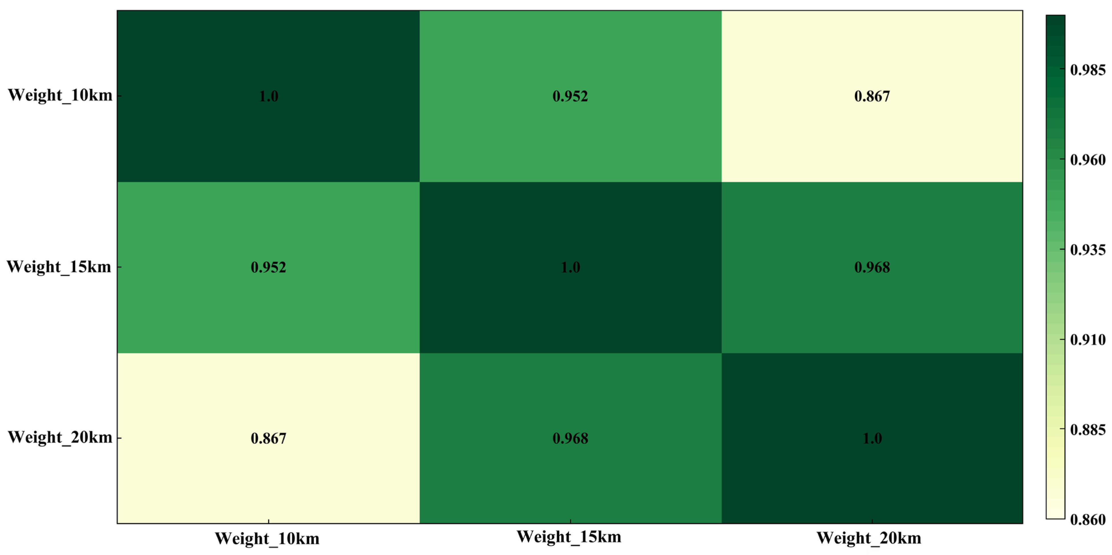
A multi-scale sensitivity analysis was conducted by comparing 10 km, 15 km, and 20 km candidate scales (Table A1, Figure A1 and Figure A2). The 10 km grid contains only 100 pixels per unit, which is insufficient for stable landscape metric and RCS threshold computation and produces 1827 units that are excessively granular for provincial macro-zoning; its CFCI distribution has a thickened low-value tail (Figure A2). The 20 km grid (400 pixels per unit, 534 units) over-smooths spatial heterogeneity (CV = 40.705%) and upward-compresses the low-fragmentation range, obscuring the structural contrasts among Jilin’s geomorphological subregions. The 15 km grid offers 225 pixels per unit—sufficient for stable metric computation—and yields the most symmetric, full-spectrum CFCI distribution (CV = 46.363%; Figure A2). Critically, the pairwise correlation matrix of CFCI weights across the three scales (Figure A1) shows that the 15 km result is highly consistent with both the 10 km (r = 0.952) and 20 km (r = 0.968) outputs, while the 10 km–20 km consistency drops to 0.867, confirming that the 15 km grid occupies the most stable intermediate position in the scale continuum. This scale uniquely preserves Jilin’s tripartite regional heterogeneity—the eastern Changbai mountainous region, the central Songnen Plain, and the western agro-pastoral ecotone. A finer grid would over-fragment the central plain and weaken cross-regional comparability, whereas a coarser grid would aggregate ecologically distinct western patches with eastern mountainous parcels, masking the heterogeneity this study aims to characterize. Furthermore, the 884 units at 15 km (225 km2 per cell) align with the township-level operational scale at which cropland regulation policies are implemented in Jilin Province. The 15 km grid was therefore selected as the optimal balance among inter-scale consistency, sample adequacy, regional heterogeneity preservation, and policy operability.
Table A1. Multi-scale sensitivity comparison of cropland fragmentation evaluation units (year 2023 as representative).
Grid ScaleEffective GridsMinimumMaximumMeanCVNumber of Pixels per Unit Grid
10 km18270.0000.6120.29654.364%100
15 km8840.0130.5760.32446.363%225
20 km5340.0300.5620.33340.705%400
Figure A1. Pearson correlation plots for the CRITIC method at different scales.
Remotesensing 18 01617 g0a1
Figure A2. Whisker plots of the CFCI at different scales.
Remotesensing 18 01617 g0a2

Appendix A.2

The parameter settings for habitat quality in the InVEST model used in this study.
Table A2. Threats Table.
Threat FactorsMaximum Distance (m)WeightDecay
Cropland30000.6linear
Impervious100001exponential
Barren20000.4linear
Table A3. Sensitivity Table.
Land Use TypeHabitat SuitabilityThreat Factors
CroplandImperviousBarren
Cropland0.300.70.3
Forest10.70.90.5
Grassland0.80.60.80.4
Water0.80.40.70.3
Impervious0000
Barren0.1000

Appendix A.3

The parameter settings for habitat quality in the PLUS model [63] used in this study are shown in Table A4. Neighborhood weights range from 0 to 1 and are used to quantify the expansion capacity of each land-use type. In line with recommendations from existing research [64], the resulting weights, as shown in Table A5, reflect the historical expansion intensity observed in Jilin Province. The transition matrix (Table A6) was configured scenario-by-scenario, following the rule-based approach [65,66]: Natural development scenario: The mutual non-conversion between water and forest is due to a lack of historical succession pathways, while the mutual non-conversion between impervious land and water is attributed to development costs and ecological protection constraints. Cropland protection scenario: Transitions from cropland to other land uses are prohibited (set to 0), consistent with China’s “Cropland Red Line” policy. Ecological protection scenario: Transitions from forest, grassland, and water to impervious land are prohibited, in line with the Ecological Protection Redline framework.
Table A4. Parameter settings of PLUS model.
ParameterSetting
Patch generation threshold0.7
Expansion coefficient0.5
Percentage of seeds0.1
Neighborhood size15
Table A5. Neighborhood weight parameters.
Land Use Type Cropland Forest Grassland Water Impervious Barren
Neighborhood weight0.7710.1610.3100.2210.3610.510
Table A6. Multi-scenario land use transition cost matrix.
Land Use TypeNatural Development ScenarioCropland Protection ScenarioEcological Protection Scenario
abcdefabcdefabcdef
a111111100000111010
b111011111011010000
c111111111111011100
d101101101111111100
e111011001010001110
f111111111111111111
Note: a, b, c, d, e, and f denote cropland, forest, grassland, water, impervious, and barren, respectively, while 0 denotes prohibited transitions, and 1 denotes permitted transitions.
Table A7. The standard deviations and CVs obtained after running the PLUS model 20 times.
Number of TrialsLand Use Type (km2)PLUS Model
CroplandForestGrasslandWaterImperviousBarrenKappaOverallFoM
190,01882,23161791749893718940.8650.9200.101
290,01882,23162371691893718940.8670.9220.102
390,01882,23162011727893718940.8570.9160.102
490,01882,23161701758893718940.8560.9140.102
589,91382,23162831750893718940.8660.9200.100
690,01882,23162031725893718940.8670.9210.101
790,01882,23162431685893718940.8600.9170.101
890,01882,23162081720893718940.8560.9140.101
990,01882,23162341694893718940.8670.9220.101
1090,01882,23162241704893718940.8630.9190.101
1190,01882,23162431685893718940.8610.9170.102
1290,01882,23161541774893718940.8600.9180.101
1390,01882,23162131715893718940.8550.9140.101
1489,89282,23162821772893718940.8640.9200.100
1590,01882,23161891739893718940.8560.9140.101
1690,01882,23162501678893718940.8590.9170.102
1790,01882,23161881740893718940.8610.9180.101
1890,01882,23162311697893718940.8550.9140.100
1990,01882,23161451783893718940.8470.9110.101
2090,01882,23162491679893718940.8620.9180.100
Mean90,00682,23162161723893718940.8600.9170.101
Standard Deviation3603834000.0050.0030.001
CV0.040%0.000%0.617%1.957%0.000%0.000%0.605%0.336%0.679%
Figure A3. Stability of the PLUS model after 20 runs.
Remotesensing 18 01617 g0a3
Table A8. Regional transfer matrices under multiple scenarios in 2023–2030 (km2).
2023Natural Development ScenarioCropland Protection ScenarioEcological Protection Scenario
z1z2z3z4z1z2z3z4z1z2z3z4
z18887.642790.37//8379.213298.80//9112.642565.37//
z2750.1588,182.881440.681045.08750.1586,607.881182.262878.50750.1588,352.39821.171495.08
z3/2371.043076.462400.90/2146.042342.743359.62/2821.042387.972639.38
z4/1837.071536.7876,722.33/1387.072518.6676,190.45/1837.072092.3776,166.74
Note: z1, z2, z3, z4 denote uncultivated zone, ecosystem landscape trade-off zone, dysfunctional sensitive zone, production-ecology synergy zone.

References

  1. Chen, Y.; Yao, M.; Zhao, Q.; Chen, Z.; Jiang, P.; Li, M.; Chen, D. Delineation of a basic farmland protection zone based on spatial connectivity and comprehensive quality evaluation: A case study of Changsha City, China. Land Use Policy 2021, 101, 105145. [Google Scholar] [CrossRef]
  2. Foley, J.A.; Ramankutty, N.; Brauman, K.A.; Cassidy, E.S.; Gerber, J.S.; Johnston, M.; Mueller, N.D.; O’Connell, C.; Ray, D.K.; West, P.C. Solutions for a cultivated planet. Nature 2011, 478, 337–342. [Google Scholar] [CrossRef]
  3. Kopittke, P.M.; Menzies, N.W.; Wang, P.; McKenna, B.A.; Lombi, E. Soil and the intensification of agriculture for global food security. Environ. Int. 2019, 132, 105078. [Google Scholar] [CrossRef]
  4. Liu, J.Y.; Kuang, W.; Zhang, Z.; Xu, X.; Qin, Y.; Ning, J.; Zhou, W.; Zhang, S.; Li, R.; Yan, C.; et al. Spatiotemporal characteristics, patterns, and causes of land-use changes in China since the late 1980s. J. Geogr. Sci. 2014, 24, 195–210. [Google Scholar] [CrossRef]
  5. Di Falco, S.; Penov, I.; Aleksiev, A.; Van Rensburg, T.M. Agrobiodiversity, farm profits and land fragmentation: Evidence from Bulgaria. Land Use Policy 2010, 27, 763–771. [Google Scholar] [CrossRef]
  6. Niroula, G.S.; Thapa, G.B. Impacts and causes of land fragmentation, and lessons learned from land consolidation in South Asia. Land Use Policy 2005, 22, 358–372. [Google Scholar] [CrossRef]
  7. Qiu, L.; Zhu, J.; Pan, Y.; Wu, S.; Dang, Y.; Xu, B.; Yang, H. The positive impacts of landscape fragmentation on the diversification of agricultural production in Zhejiang Province, China. J. Clean. Prod. 2020, 251, 119722. [Google Scholar] [CrossRef]
  8. Zang, L.; Araral, E.; Wang, Y. Effects of land fragmentation on the governance of the commons: Theory and evidence from 284 villages and 17 provinces in China. Land Use Policy 2019, 82, 518–527. [Google Scholar] [CrossRef]
  9. Xu, K.; Yi, X.; Zhou, L. Impacts of agricultural production services on green grain production efficiency: Factors allocation perspective. J. Environ. Manag. 2025, 380, 125136. [Google Scholar] [CrossRef]
  10. Meng, L.; Yan, F. Research on the impact mechanism of comprehensive land consolidation on rural human settlement environment based on the production-living-ecological space theory: A case study of Zhejiang Province, China. Front. Public Health 2025, 13, 1633895. [Google Scholar] [CrossRef]
  11. Janus, J.; Markuszewska, I. Forty years later: Assessment of the long-lasting effectiveness of land consolidation projects. Land Use Policy 2019, 83, 22–31. [Google Scholar] [CrossRef]
  12. Peiheng, Y.; Shailaja, F.; Yiyun, C.; Hui, L.; Lu, X.; Jiawei, P.; Shaoyun, B.; Shixiang, G. Positive impacts of farmland fragmentation on agricultural production efficiency in Qilu Lake watershed: Implications for appropriate scale management. Land Use Policy 2022, 117, 106108. [Google Scholar] [CrossRef]
  13. Tran, T.Q.; Vu, H.V. Land fragmentation and household income: First evidence from rural Vietnam. Land Use Policy 2019, 89, 104247. [Google Scholar] [CrossRef]
  14. Latruffe, L.; Piet, L. Does land fragmentation affect farm performance? A case study from Brittany, France. Agric. Syst. 2014, 129, 68–80. [Google Scholar] [CrossRef]
  15. Wen, G.; Wang, X.; Hu, X.; Xia, W. Impact of cultivated land scale and fragmentation on chemical fertilizer non-point source pollution. Chin. J. Eco-Agric. 2023, 31, 1081–1093. [Google Scholar]
  16. Li, F.; Jiang, Y.; Wu, L.; Zhang, Z. Spatial and temporal dynamics of fragmentation and an ecosystem health assessment of plateau blue landscapes: A case study of the Caohai wetland. Catena 2025, 250, 108730. [Google Scholar] [CrossRef]
  17. Wei, Y.; Chen, Y.; Wang, J.; Yu, P.; Xu, L.; Zhang, C.; Shen, H.; Liu, Y.; Zhang, G. Mapping soil organic carbon in fragmented agricultural landscapes: The efficacy and interpretability of multi-category remote sensing variables. J. Integr. Agric. 2025, 24, 4395–4414. [Google Scholar] [CrossRef]
  18. Mauda, E.V.; Joseph, G.S.; Seymour, C.L.; Munyai, T.C.; Foord, S.H. Changes in landuse alter ant diversity, assemblage composition and dominant functional groups in African savannas. Biodivers. Conserv. 2018, 27, 947–965. [Google Scholar] [CrossRef]
  19. Bagella, S.; Caria, M.C.; Seddaiu, G.; Leites, L.; Roggero, P.P. Patchy landscapes support more plant diversity and ecosystem services than wood grasslands in Mediterranean silvopastoral agroforestry systems. Agric. Syst. 2020, 185, 102945. [Google Scholar] [CrossRef]
  20. Deng, O.; Ran, J.; Huang, S.; Duan, J.; Reis, S.; Zhang, J.; Zhu, Y.-G.; Xu, J.; Gu, B. Managing fragmented croplands for environmental and economic benefits in China. Nat. Food 2024, 5, 230–240. [Google Scholar] [CrossRef]
  21. Ingo, G.; Jacqueline, L.; Svenja, B.; Péter, B.; Felipe, L.; Anoush, F.; Felix, K.; Maraja, R.; Julia, R.; Julia, T.; et al. Land-sharing/-sparing connectivity landscapes for ecosystem services and biodiversity conservation. People Nat. 2019, 1, 262–272. [Google Scholar] [CrossRef]
  22. Martin, E.A.; Matteo, D.; Yann, C.; András, B.; Riccardo, B.; Vesna, G.; Garratt, M.P.D.; Andrea, H.; David, K.; Anikó, K.-H.; et al. The interplay of landscape composition and configuration: New pathways to manage functional biodiversity and agroecosystem services across Europe. Ecol. Lett. 2019, 22, 1083–1094. [Google Scholar] [CrossRef]
  23. Liu, Q.; Sun, X.; Huang, Q.; Qiao, J.; Fang, G.; Ren, Y.; Wang, C.; Sun, J.; Yang, P. Optimizing the landscape in grain production and identifying trade-offs between ecological benefits based on production possibility frontiers: A case study of Beijing-Tianjin-Hebei region. J. Environ. Manag. 2025, 377, 124583. [Google Scholar] [CrossRef]
  24. Jian, P.; Xiaoyu, W.; Huining, Z.; Zihan, X. Applying production-possibility frontier based ecosystem services trade-off to identify optimal scenarios of Grain-for-Green Program. Landsc. Urban Plan. 2024, 242, 104956. [Google Scholar] [CrossRef]
  25. Wang, Y.; He, Y.; Fan, J.; Olsson, L.; Scown, M. Balancing urbanization, agricultural production and ecological integrity: A cross-scale landscape functional and structural approach in China. Land Use Policy 2024, 141, 107156. [Google Scholar] [CrossRef]
  26. Liu, F.; Hu, W.; Min, M.; Liu, T.; Li, S.; Rong, Q. How does road networks impact cultivated land multifunctionality? The role of land fragmentation: Evidence from Hubei Province, China. Front. Sustain. Food Syst. 2025, 9, 1686176. [Google Scholar] [CrossRef]
  27. Su, S.; Yang, C.; Hu, Y.; Luo, F.; Wang, Y. Progressive landscape fragmentation in relation to cash crop cultivation. Appl. Geogr. 2014, 53, 20–31. [Google Scholar] [CrossRef]
  28. Li, Y.; Wu, W.; Liu, Y. Land consolidation for rural sustainability in China: Practical reflections and policy implications. Land Use Policy 2018, 74, 137–141. [Google Scholar] [CrossRef]
  29. Ntihinyurwa, P.D.; Vries, W.T.d.; Chigbu, U.E.; Dukwiyimpuhwe, P.A. The positive impacts of farm land fragmentation in Rwanda. Land Use Policy 2019, 81, 565–581. [Google Scholar] [CrossRef]
  30. Liang, J.; Pan, S.; Chen, W.; Li, J.; Zhou, T. Cultivated Land Fragmentation and Its Influencing Factors Detection: A Case Study in Huaihe River Basin, China. Int. J. Environ. Res. Public Health 2021, 19, 138. [Google Scholar] [CrossRef]
  31. Liu, J.; Jin, X.; Xu, W.; Sun, R.; Han, B.; Yang, X.; Gu, Z.; Xu, C.; Sui, X.; Zhou, Y. Influential factors and classification of cultivated land fragmentation, and implications for future land consolidation: A case study of Jiangsu Province in eastern China. Land Use Policy 2019, 88, 104185. [Google Scholar] [CrossRef]
  32. Looga, J.; Jürgenson, E.; Sikk, K.; Matveev, E.; Maasikamäe, S. Land fragmentation and other determinants of agricultural farm productivity: The case of Estonia. Land Use Policy 2018, 79, 285–292. [Google Scholar] [CrossRef]
  33. Tu, Y.; Chen, B.; Yu, L.; Xin, Q.; Gong, P.; Xu, B. How does urban expansion interact with cropland loss? A comparison of 14 Chinese cities from 1980 to 2015. Landsc. Ecol. 2020, 36, 243–263. [Google Scholar] [CrossRef]
  34. Jiang, P.; Li, M.; Cheng, L. Dynamic response of agricultural productivity to landscape structure changes and its policy implications of Chinese farmland conservation. Resour. Conserv. Recycl. 2020, 156, 104724. [Google Scholar] [CrossRef]
  35. Ishiyama, N.; Sueyoshi, M.; Watanabe, N.; Nakamura, F. Biodiversity and rarity distributions of native freshwater fish in an agricultural landscape: The importance of beta diversity between and within water-body types. Aquat. Conserv. Mar. Freshw. Ecosyst. 2016, 26, 416–428. [Google Scholar]
  36. Kong, X. China must protect high-quality arable land. Nature 2014, 506, 7. [Google Scholar] [CrossRef]
  37. Wang, J. Land Management Scale, Fragmentation and Grain Production Efficiency. Times Agric. Mach. 2017, 44, 170. [Google Scholar]
  38. Yao, Y.; Zhang, Y. How Can the “National Granary” be Stable?——The Era Analysis Based on Food Security in Northeast China. Theor. Investig. 2026, 12–19. [Google Scholar] [CrossRef]
  39. Cao, Y.; Zou, J.; Fang, X.; Wang, J.; Cao, Y.; Li, G. Effect of land tenure fragmentation on the decision-making and scale of agricultural land transfer in China. Land Use Policy 2020, 99, 104996. [Google Scholar] [CrossRef]
  40. Wang, X.; Su, X. The Impact of Agricultural Land Fragmentation on Agricultural Production: A Case Study of Laixi City, Shandong Province. J. Agrotech. Econ. 2002, 2, 2–7. [Google Scholar] [CrossRef]
  41. Yang, J.; Huang, X. The 30m annual land cover dataset and its dynamics in China from 1990 to 2019. Earth Syst. Sci. Data 2021, 13, 3907–3925. [Google Scholar] [CrossRef]
  42. Yu, H.; Jiang, H.; Liu, J.; Zhang, S.; Fan, M.; Feng, X. Multiscale patterns and future dynamics of cultivated land fragmentation in Northeast China. J. Environ. Manag. 2026, 399, 128539. [Google Scholar] [CrossRef]
  43. Fengkui, Q.; Yanru, C.; Rattan, L.; Klaus, L. Spatio-temporal characteristics of cultivated land fragmentation in different landform areas with a case study in Northeast China. Ecosyst. Health Sustain. 2020, 6, 1800415. [Google Scholar] [CrossRef]
  44. Diakoulaki, D.; Mavrotas, G.; Papayannakis, L. Determining objective weights in multiple criteria problems: The critic method. Comput. Oper. Res. 1995, 22, 763–770. [Google Scholar] [CrossRef]
  45. Chen, J.; Xu, C.; Li, K.; Song, M. A gravity model and exploratory spatial data analysis of prefecture-scale pollutant and CO2 emissions in China. Ecol. Indic. 2018, 90, 554–563. [Google Scholar] [CrossRef]
  46. Brody, S.D.; Zahran, S.; Grover, H.; Vedlitz, A. A spatial analysis of local climate change policy in the United States: Risk, stress, and opportunity. Landsc. Urban Plan. 2008, 87, 33–41. [Google Scholar] [CrossRef]
  47. Kanaroglou, P.S.; Adams, M.D.; Luca, P.F.D.; Corr, D.; Sohel, N. Estimation of sulfur dioxide air pollution concentrations with a spatial autoregressive model. Atmos. Environ. 2013, 79, 421–427. [Google Scholar] [CrossRef]
  48. Shi, L.; Halik, U.; Mamat, Z.; Aishan, T.; Abliz, A.; Welp, M. Spatiotemporal investigation of the interactive coercing relationship between urbanization and ecosystem services in arid northwestern China. Land Degrad. Dev. 2021, 32, 4105–4120. [Google Scholar] [CrossRef]
  49. Zhou, D.Y.; Tian, Y.Y.; Jiang, G.H. Spatio-temporal investigation of the interactive relationship between urbanization and ecosystem services: Case study of the Jingjinji urban agglomeration, China. Ecol. Indic. 2018, 95, 152–164. [Google Scholar] [CrossRef]
  50. Lu, M.; Zhang, Y.; Liang, F.; Wu, Y. Spatial Relationship between Land Use Patterns and Ecosystem Services Value-Case Study of Nanjing. Land 2022, 11, 1168. [Google Scholar] [CrossRef]
  51. Xiao, G.; Zhu, X.; Hou, C.; Liu, Y.; Xu, K. A spatialization method for grain yield statistical data: A study on winter wheat of Shandong Province, China. Agron. J. 2019, 111, 1892–1903. [Google Scholar] [CrossRef]
  52. Fuentes, I.; Al-Shammari, D.; Al-Nasrawi, A.K.; Wang, Y.; Wang, J.; Lebrini, Y.; Chen, Y.; Jones, B.G.; Bishop, T.F. The normalised difference vegetation index as an analytic tool for wheat crop yield prediction: A review and meta-analysis. Precis. Agric. 2025, 26, 55. [Google Scholar] [CrossRef]
  53. Belmahi, M.; Hanchane, M.; Krakauer, N.Y.; Kessabi, R.; Bouayad, H.; Mahjoub, A.; Zouhri, D. Analysis of Relationship between Grain Yield and NDVI from MODIS in the Fez-Meknes Region, Morocco. Remote Sens. 2023, 15, 2707. [Google Scholar] [CrossRef]
  54. Hassan, M.A.; Yang, M.; Rasheed, A.; Yang, G.; Reynolds, M.; Xia, X.; Xiao, Y.; He, Z. A rapid monitoring of NDVI across the wheat growth cycle for grain yield prediction using a multi-spectral UAV platform. Plant Sci. 2019, 282, 95–103. [Google Scholar] [CrossRef]
  55. Xie, M.; He, T.; Fan, S.; Weng, Y.; Huang, W.; Zhang, M. Characteristics of the Spatial and Temporal Evolution of Arable Land Resources and Production Capacity in Three Northeastern Provinces from 2000 to2020. Chin. J. Soil Sci. 2024, 55, 1205–1214. [Google Scholar] [CrossRef]
  56. Deng, G.; Liu, Y.; Jiang, H.; Zhu, S.; Wen, Y.; Sheng, L.; Guo, Y. Disentangling the relative and cumulative impacts of diverse policies on food- and water-related ecosystem services and their trade-offs in ecologically fragile areas. J. Clean. Prod. 2024, 447, 141322. [Google Scholar] [CrossRef]
  57. Zhao, L.; Li, K.; Liu, Z.; Shao, D.; Chen, Q.; Zhu, Y.; Han, F. Spatiotemporal dynamics of soil erosion and its interactive mechanisms with NDVI in the Yellow River Basin, China. J. Environ. Manag. 2026, 402, 129016. [Google Scholar] [CrossRef]
  58. Bai, X.; Lin, C.; Wang, S.; Xiong, J.; Xu, J.; Xue, K.; Ma, D.; Tong, Y.; Chen, J.; Cui, W. Ponds greatly influence watershed ecosystem services value: An optimized InVEST model for large-scale. J. Hydrol. 2026, 668, 135026. [Google Scholar] [CrossRef]
  59. Jiao, L. Urban land density function: A new method to characterize urban expansion. Landsc. Urban Plan. 2015, 139, 26–39. [Google Scholar] [CrossRef]
  60. Discacciati, A.; Palazzolo, M.G.; Park, J.G.; Melloni, G.E.M.; Murphy, S.A.; Bellavia, A. Estimating and presenting non-linear associations with restricted cubic splines. Int. J. Epidemiol. 2025, 54, dyaf088. [Google Scholar] [CrossRef]
  61. Wu, Z.; Dou, X.; Li, X.; Cao, M.; Ouyang, H.; Xia, F. Age Modifies the Prognostic Impact of Sex in Follicular Thyroid Carcinoma: A SEER Database Analysis. Ann. Surg. Oncol. 2026, 1–10. [Google Scholar] [CrossRef]
  62. Geng, J.; Li, L.; Guo, S.; Cheng, M.; Qu, B.; Huang, J. Spatio-temporal Evolution and Multi-scenario Prediction of Ecosystem Service Valueof Resource-based Cities in Henan Province Based on PLUS Model. Environ. Sci. 2025, 46, 7878–7888. [Google Scholar] [CrossRef]
  63. Liang, X.; Guan, Q.; Clarke, K.C.; Liu, S.; Wang, B.; Yao, Y. Understanding the drivers of sustainable land expansion using a patch-generating land use simulation (PLUS) model: A case study in Wuhan, China. Comput. Environ. Urban Syst. 2021, 85, 101569. [Google Scholar] [CrossRef]
  64. Liu, J.; Kong, X.; Zhu, Y.; Zhang, B. A study on land use change simulation based on PLUS model and the U-net structure: A case study of Jilin Province. Ecol. Indic. 2025, 176, 113619. [Google Scholar] [CrossRef]
  65. Jing, G.; Hongyan, D.; Yong, S.; Yun, Z. Simulation and prediction of land use in urban agglomerations based on the PLUS model: A case study of the Pearl River Delta, China. Front. Environ. Sci. 2023, 11, 1306187. [Google Scholar] [CrossRef]
  66. Zhao, C.; Wu, S.; Yang, L.; Wu, Y.; Xiao, P.; Xu, J.; Liu, Y. Evaluating ecological conservation effectiveness of security patterns under multiple scenarios: A case study of Hubei Province. Ecol. Indic. 2024, 166, 112528. [Google Scholar] [CrossRef]
  67. Pontius, R.G.; Boersma, W.; Castella, J.-C.; Clarke, K.; Nijs, T.; Dietzel, C.; Duan, Z.; Fotsing, E.; Goldstein, N.; Kok, K.; et al. Comparing the input, output, and validation maps for several models of land change. Ann. Reg. Sci. 2008, 42, 11–37. [Google Scholar] [CrossRef]
  68. Xu, B.; Zhang, W.; Wu, B. Identification of Ecosystem Service Degradation Risks and Regulation Pathwaysalong the Pinglu Canal Based on Multi-scenario Simulations of Land-use Change. Environ. Sci. 2026, 1–26. [Google Scholar] [CrossRef]
  69. Zhang, J.; Fu, H.; Fu, Y.; Xu, D.; Chen, W.; Kang, B.; Ma, B.; Wang, Z. Current Status of Habitat Quality in Xiliugou Basin Based on InVEST Model. J. Soil Water Conserv. 2025, 39, 331–341. [Google Scholar] [CrossRef]
  70. Brudvig, L.A.; Damschen, E.I.; Tewksbury, J.J.; Haddad, N.M.; Levey, D.J. Landscape connectivity promotes plant biodiversity spillover into non-target habitats. Proc. Natl. Acad. Sci. USA 2009, 106, 9328–9332. [Google Scholar] [CrossRef]
  71. Zeng, Z.; He, P. How does the high standard farmland construction affect the efficiency of grain production? J. Arid Land Resour. Environ. 2025, 39, 94–104. [Google Scholar] [CrossRef]
  72. Malin, T.; Erik, Ö.; Therese, L.; Pettersson, L.B.; Smith, H.G.; Martin, S.; Thomas, R. Land sharing complements land sparing in the conservation of disturbance-dependent species. Ambio 2022, 52, 571–584. [Google Scholar] [CrossRef]
Figure 1. Location of the study area (a), land use of the study area (b), elevation and administrative districts of the study area (c).
Remotesensing 18 01617 g001
Figure 2. Research framework.
Remotesensing 18 01617 g002
Figure 3. Spatial distribution of cropland fragmentation in Jilin Province from 2000 to 2023.
Remotesensing 18 01617 g003
Figure 4. Spatial aggregation distribution in Jilin Province from 2000 to 2023.
Remotesensing 18 01617 g004
Figure 5. Spatial distribution of grain yield, annual water yield, sediment delivery ratio, and habitat quality in Jilin Province from 2000 to 2023.
Remotesensing 18 01617 g005
Figure 6. Nonlinear relationships between cropland fragmentation and annual water yield (a), sediment delivery ratio (b), and habitat quality (c), ecosystem (d), and grain yield (e).
Remotesensing 18 01617 g006
Figure 7. Spatial distribution of cropland fragmentation and multifunctional effects in Jilin Province in 2023.
Remotesensing 18 01617 g007
Figure 8. The relative contributions of different factors to land-use expansion.
Remotesensing 18 01617 g008
Figure 9. Predicted compared to actual land use status for Jilin Province in 2020.
Remotesensing 18 01617 g009
Figure 10. Spatial distribution map of multifunctional effects under different scenario simulations in Jilin Province.
Remotesensing 18 01617 g010
Figure 11. Evolution of structure of cropland fragmentation multifunctional zoning in Jilin Province under different scenario simulations.
Remotesensing 18 01617 g011
Table 1. Data acquisition.
DataFormatResolutionData Sources
Digital Elevation ModelTiff30 mhttps://www.gscloud.cn/, (accessed on 10 November 2025)
Land use dataTiff30 mChina Land Cover Dataset (CLCD) [41]
GDPTiff1000 mResource and Environment Science and Data Center
Population densityTiff1000 mhttps://www.worldpop.org/, (accessed on 15 November 2025)
NDVITiff250 mhttps://data.tpdc.ac.cn/home
https://doi.org/10.11888/Terre.tpdc.300330, (accessed on 20 October 2025)
Precipitation/potential evapotranspirationNETCDF1000 mNational Earth System Science Data Center
Road data (motorways, primary roads, secondary and tertiary roads)
Railway
Shp/https://www.openstreetmap.org, (accessed on 1 November 2025)
TemperatureNETCDF1000 mNational Earth System Science Data Center
Grain yield/tJilin Statistical Yearbook
Soil dataShp1:1,000,000http://www.fao.org/soils-portal/soil-survey/soil-maps-and-databases/harmonized-world-soil-database-v12/en/, (accessed on 15 June 2025)
Root-restricting layer depthRaster1000 mhttps://doi.org/10.1038/s41597-019-0345-6, (accessed on 17 November 2025)
Table 2. Indicators and weights for assessing cropland fragmentation in Jilin Province.
IndicatorVifToleranceDirectionWeighting
NP2.300.44+14.54
PD1.280.78+3.40
ED8.260.12+12.33
AWMSI7.660.13+12.38
SPLIT2.100.48+14.49
AREA_MN2.870.3524.67
COHESION4.780.2118.19
Note: The VIF values of ED and AWMSI are slightly above 5 due to their inherent geometric relationship concerning patch perimeter and area. The CRITIC method accounts for indicator conflict, ensuring moderate collinearity does not compromise index reliability.
Table 3. Global Moran’s I index of cropland fragmentation.
YearMoran’s IZ-Valuep-Value
20000.752 ***39.6000.001
20100.730 ***38.9130.001
20230.739 ***40.4750.001
Note: In the table, *** indicates significance at the 1% level of probability.
Table 4. Threshold effect results of cropland fragmentation on production and ecological functions.
TypeR2Threshold
CFCI-GY0.6420.340
CFCI-AWY0.9890.363
CFCI-SDR0.6040.363
CFCI-HQ0.4570.363
CFCI-ES0.7300.363
Disclaimer/Publisher’s Note: The statements, opinions and data contained in all publications are solely those of the individual author(s) and contributor(s) and not of MDPI and/or the editor(s). MDPI and/or the editor(s) disclaim responsibility for any injury to people or property resulting from any ideas, methods, instructions or products referred to in the content.