Article

Robust Hyperspectral Anomaly Detection via Unsupervised Multiscale Feature Fusion
1
School of the Computer and Artificial Intelligence, Liaoning Normal University, Dalian 116029, China
2
School of Information Science and Engineering, Northeastern University, Shenyang 110167, China
3
School of Information Engineering, Dalian University, Dalian 116622, China
4
School of Geographical Sciences, Liaoning Normal University, Dalian 116029, China
*
Author to whom correspondence should be addressed.
Remote Sens. 2026, 18(10), 1554; https://doi.org/10.3390/rs18101554
Submission received: 21 March 2026 / Revised: 28 April 2026 / Accepted: 3 May 2026 / Published: 13 May 2026
(This article belongs to the Special Issue Recent Progress in Hyperspectral Remote Sensing Data Processing)

Highlights

What are the main findings?
  • A robust unsupervised multi-scale feature fusion network (UMF2Net) is developed for HSI-AD.
  • Central difference convolution and 3D convolution feature weighting are integrated to capture multi-scale spatial-spectral signatures.
What are the implications of the main findings?
  • By effectively fusing hierarchical features, UMF2Net achieved competitive results in four different remote sensing scenarios.
  • The framework provides a robust solution for detecting anomalies of varying sizes without requiring prior target information.

Abstract

In hyperspectral image (HSI) anomaly detection (AD) methods, detecting small targets or anomalies remains challenging. This difficulty arises because targets or anomalies may vary significantly in size, shape, and texture, causing them to be obscured by larger-scale background features. To address the above issue, this paper proposes an unsupervised multi-scale feature fusion network (UMF2Net) for HSI-AD. Firstly, central difference convolution analyzes the image at multiple scales to capture fine-to-coarse details and structural information. Additionally, three-dimensional (3D) convolution is employed to generate feature weights for the multi-scale features, assigning different weights to features with different contributions so that the model dynamically emphasizes features that have a greater impact on the AD results. Finally, by using the two proposed multi-scale feature fusion modules, the model effectively integrates features at different scales, thereby enhancing its ability to detect anomalies of varying sizes. Compared with several classical HSI-AD algorithms on real hyperspectral datasets from four scenarios, UMF2Net achieved competitive detection results, verifying the effectiveness of our algorithm.

1. Introduction

Hyperspectral image (HSI) anomaly detection (AD) aims to distinguish anomalies from the background. To achieve this goal, it is usually necessary to extract background information from the image and use the differences between the background and anomaly for differentiation. With the rapid development of hyperspectral imaging technology, HSI-AD has been widely applied in various fields, including military target camouflage [1], border monitoring [2], mineral detection [3], precision agriculture [4], and urban monitoring [5]. Over the past two decades, numerous outstanding models and methods have been developed in the field of AD for hyperspectral remote sensing images. Furthermore, the application of hyperspectral imaging is evolving from static scene analysis toward dynamic target monitoring [6]. Specifically, hyperspectral target tracking has emerged as a frontier research hotspot in recent years, fully leveraging the extremely high spectral resolution of hyperspectral imagery. Compared with traditional color-based trackers, hyperspectral trackers demonstrate superior robustness and discriminative power when handling challenging tasks such as extreme similarity between target and background colors, drastic illumination variations, and complex occlusions [7]. The vigorous development of this emerging field not only strongly validates the core value of spectral-dimensional features in complex scene understanding but also provides significant references and broad prospects for the application of hyperspectral anomaly detection in real-time dynamic early warning and continuous surveillance [8]. The statistical model-based RX anomaly detector was introduced by Reed and Yu [9] and has become an industry standard for HSI-AD. Many enhanced algorithms based on RX have also been proposed. Examples include Local RX (LRX) [10], Kernel RX (KRX) [11], and Cluster Kernel RX (CKRX) [12]. Although the aforementioned methods have achieved remarkable results, their performance in complex scenarios remains unsatisfactory. In recent years, sparse representation-based HSI-AD algorithms have been proposed extensively and have shown promising results. However, the sparse representation theory primarily captures local structural information, while the sparsity of signals corresponds to a low-rank property globally in HSIs. In combining the advantages of both, a series of HSI-AD algorithms based on low-rank sparse representation have been proposed, such as the dictionary reconstruction and anomaly extraction algorithm based on low-rank sparse matrix factorization proposed by Xu et al. [13]. They treated HSIs as consisting of a low-rank background, noise, and an anomalies. The Godec algorithm has been used to quickly and iteratively solve the optimization problem. However, it often mistakes anomalies for noise, which reduces the anomaly identification rate. Ruhan et al. introduced the Mahalanobis distance method based on enhanced tensor RPCA [14] into HSI-AD. They divided the image into low-rank and sparse subspaces and solved the convex optimization problem through appropriate relaxation. Although the above methods have improved the performance of HSI-AD to some extent, the single subspace model used in the above algorithms struggles to accurately describe the image background due to the complex ground information contained in HSIs. To address the mentioned issue, Wang et al. suggested an HSI-AD algorithm based on unmixing fusion and a background sparse dictionary [15]. By obtaining the abundance matrix through hyperspectral unmixing and fusing it with an HSI, the spatial information of the HSI was supplemented to a certain extent. Liu et al. proposed a multi-scale network with a self-supervised learning mechanism, which significantly improved the performance of HSI-AD under the self-supervision framework, especially in complex scenes and multi-scale object detection.
Deep learning (DL), a cutting-edge area, has recently provided viable solutions to numerous pattern recognition problems. The two types of DL frameworks are supervised learning and unsupervised learning. A key criterion for categorizing these models is whether an annotated training dataset is required. As an unsupervised object detection method, HSI-AD does not require prior target information. Jiang et al. developed a low-rank embedded network for sample-free HSI-AD by extracting latent features from autoencoders [16]. Wang et al. proposed an HSI-AD method based on the attention gate connected fully convolutional autoencoder, which better identified anomalies by assigning higher weights to the background [17]. Li et al. introduced a multi-scale attribute and edge-preserving filtering method [18]. That study significantly improved the detection performance for multi-scale anomalous targets in complex scenes by integrating multi-scale attribute filtering and combining it with SVM classification. Liu et al. [19] designed a multi-scale network with self-supervision function, which notably boosted the performance of HSI-AD, particularly in complex scenes and multi-scale object detection. Wang et al. [20] proposed a GAN-based detection model based on variational background inference. This method introduces variational inference to converge the background distribution to a multivariate normal distribution and utilizes coupling loss to enforce feature matching between two discriminators. This approach effectively addresses the challenge of accurately modeling background distributions in GAN-based methods, significantly enhancing the fidelity of spectral reconstruction. Zhang et al. [21] designed a joint detection model combining graph theory and deep learning. In this method, a spectral sub-model utilizes a graph Fourier transform to capture global statistical information, while a spatial sub-model extracts local spatial details via stacked autoencoders. By performing feature mapping in the fractional Fourier domain, the model effectively exploits the joint spatial-spectral features of hyperspectral imagery, overcoming the limitations of single subspace models in characterizing complex geometric structures. Sun et al. [22] introduced CSSBR, a background reconstruction framework based on contrastive self-supervised learning. This method constructs a pixel- and patch-level masking strategy and employs a dual attention network encoder, composed of a vision transformer and a channel attention module, to extract global contextual information. Driven by background reconstruction guided loss, the model achieves universal background representation learning in the absence of labeled samples, significantly reducing false alarm rates in complex scenes. Chen et al. [23] proposed a dual-window spectral diffusion model named DWSDiff. This method designs a spectral diffusion model specifically tailored to the characteristics of hyperspectral data, achieving precise background estimation through an iterative spectral diffusion and reverse reconstruction process. Furthermore, the study innovatively introduces a dual-window strategy to effectively suppress interference from anomaly extension areas within the neighborhood on background modeling, achieving state-of-the-art performance on multiple benchmark datasets such as Airport-Beach-Urban. Sun et al. [24] proposed a Mamba-enhanced background suppression diffusion model. The model incorporates the Mamba architecture, which excels at handling long-range dependencies, into a diffusion framework to capture complex global spatial-spectral features. By guiding the reverse diffusion process to dynamically erase background signals and combining a weighted loss function to mitigate training biases caused by anomalous pixels, the model provides an extremely robust solution for identifying small and hidden targets in complex landscapes. Although the aforementioned deep learning methods exhibit significant advantages in feature representation, most existing approaches still suffer from insufficient multi-scale information fusion, the loss of local spatial details, and high computational complexity. Consequently, it remains a critical challenge in current research to achieve robust detection of multi-scale and multiform anomalous targets while simultaneously ensuring model lightweightness.
Existing HSI-AD methods typically use the spectral vector of a single pixel as the network input, focusing only on spectral differences between pixels while ignoring rich local spatial information. In addition, single scale detection methods cannot simultaneously capture anomalies of different sizes and are susceptible to background interference. This paper proposes an HSI-AD method that integrates features of different scales. The main contributions are summarized as follows:
(1)
We propose an unsupervised HSI-AD network based on multi-scale feature fusion. The network extracts high-, medium-, and low-level spatial features from different neighborhoods through multi-scale central difference convolutions of different scales. Then, feature weighting is performed to emphasize informative features more effectively. Furthermore, we propose two multi-scale feature fusion methods based on attention modules, which perform deep and shallow feature fusion on the three different scale features mentioned above.
(2)
We develop a 3D convolution feature weighting module that evaluates the importance of each feature by performing feature weight calculation on the above features and applies feature weights to achieve stronger constraints or attention to useful features. Thus, the performance of the model is improved.
(3)
We introduce two multi-scale feature fusion methods. They are the spatial and channel attention fusion module and the cross-deformable attention fusion module. The spatial and channel attention fusion module simultaneously considers channel and spatial information, which can effectively enhance the model’s ability to focus on key features. The cross-deformable attention fusion module aims to enhance the representation ability of features through deformable convolution and cross-scale interaction, thereby better handling multi-scale features. These two fusion methods effectively integrate the advantages of different features, compensate for their respective shortcomings, and improve the performance of the model.
The remainder of this paper is organized as follows. Section 2 provides a comprehensive review of prior studies. Section 3 elaborates on the architecture of the proposed UMF2Net. Section 4 presents the experimental set-ups, including the description of the four hyperspectral datasets, followed by a comparative analysis of the results. The discussion and conclusions are provided in Section 5 and Section 6, respectively.

2. Related Work

2.1. RX Algorithm

The RX algorithm is a statistical model-based AD method. It assumes that the background follows a Gaussian distribution and employs a generalized likelihood ratio test to detect anomalies in hyperspectral images under a given false alarm probability. The RX algorithm can be divided into global RX and local RX. Global RX processes the entire image for AD, while local RX calculates a detection statistic based on local statistical measures (mean and covariance) within a sliding window and compares it to a predefined threshold to determine anomalies [9]:
D ( x ) = ( x μ ) T P 1 ( x μ ) δ , C 1 < δ , C 0
where μ is the mean vector of the background, P 1 is the inverse covariance matrix of the image, with their mathematical expressions given in Equations (2) and (3), respectively, δ is the decision threshold, and D ( x ) represents the Mahalanobis distance between the spectral signature of the target pixel and the mean vector of the background window. If D ( x ) exceeds or equals the detection threshold, then the pixel is classified as anomalous. The total number of pixels is denoted by N:
μ = 1 N i = 1 N x i ,
P = 1 N i = 1 N ( x i μ ) ( x i μ ) T
As a classic HSI-AD method, the RX algorithm is based on the multivariate normal distribution assumption and generalized likelihood ratio test, achieving optimal detection performance when the Gaussian distribution assumption holds. The Mahalanobis distance metric effectively accounts for inter-band correlations. Moreover, Local RX adapts to non-uniform background distributions, thereby improving detection sensitivity. However, the algorithm is highly dependent on the Gaussian assumption, with detection performance significantly degrading when data deviates from this assumption. Its computational complexity is high, especially for high-dimensional data. Although Local RX enhances adaptability, it exhibits sensitivity to the window size and incurs additional computational overhead. The threshold selection lacks an adaptive mechanism, requiring manual tuning or auxiliary analysis. Additionally, the algorithm shows better detection capability for small targets than for large ones. These limitations have motivated numerous improved versions of the RX algorithm.

2.2. Central Difference Convolution

Central difference convolution is a specialized convolutional method [25]. Unlike traditional convolution, which typically extracts only local image features, central difference convolution performs central difference operations on the input image. This enables the capture of both rich local features and subtle spectral variations, thereby improving AD accuracy. Additionally, since central difference convolution does not introduce extra parameters, it effectively avoids overfitting during training, enhancing the model’s generalization capability and making it more reliable in practical applications.
The overall process of central difference convolution can be broadly divided into two stages: sampling and aggregation. Sampling, similar to traditional convolution, extracts a patch from the input feature map with the same size as the convolution kernel. In aggregation, the central pixel is subtracted from each pixel in the patch, and the result is then processed through a standard convolution operation. The mathematical formulation is as follows:
Y ( q 0 ) = x n R w ( q m ) · x ( q 0 + q m ) x ( q 0 )
where q 0 denotes the central pixel while q m represents its neighborhood. For instance, if the kernel size is 3 × 3 , then q m corresponds to the 8 neighborhood.
To uniformly extract both intensity-level and gradient-level information, the linear blending model is adopted. The output feature of central difference convolution can be expressed as follows:
Y ( q 0 ) = λ · x n R w ( q m ) · x ( q 0 + q m ) x ( q 0 ) + ( 1 λ ) · x n R w ( q m ) · ( x ( q 0 + q m ) )
where λ [ 0 , 1 ] serves as a balancing weight to adjust the importance between the intensity and gradient levels.
Central difference convolution is an innovative approach that cleverly combines traditional convolution operations with central differential operations, demonstrating significant advantages in the field of computer vision. The core idea is to retain the feature extraction capability of traditional convolution while incorporating a central difference operation. This enhances the perception of local gradient changes, leading to more accurate capture of image details. In image classification tasks, it significantly improves the recognition of subtle textures and local features. In object detection, it shows marked improvement in accuracy, especially for small objects and low-contrast targets. In facial recognition systems, central difference convolution enhances the model’s robustness against lighting variations and subtle facial expressions. The unique gradient-enhanced feature representation mechanism enhances the network’s sensitivity to edge and texture features. Through its neighborhood difference operation, this method achieves excellent noise suppression capabilities. Moreover, the modular design allows seamless integration into existing CNN architectures without modifying the overall network structure. These advantages make it a powerful tool for improving model performance.

3. Proposed Method

This paper proposes an unsupervised network, UMF2Net, based on multi-scale feature extraction and fusion. Figure 1 illustrates the overall framework.
Assuming that there is an input image I (with dimensions C × H × W, where C, H, and W represent the number of spectral bands, height, and width of the HSI, respectively), the normalized image I ^ is obtained by normalizing I. First, we use three central difference convolutions with different scales to extract high-, medium-, and low-level spatial features from neighborhoods in the HSI. Next, feature weight calculation is applied to these features to evaluate their importance. By performing feature weighting, we impose stronger constraints or attention on useful features, thereby enhancing the model’s representation capability. Then, we propose two multi-scale feature fusion methods based on attention modules to perform deep and shallow fusion on the three scale-specific features. Finally, the fused anomaly-enhanced feature maps are processed using the RX algorithm, which improves the accuracy of HSI-AD to some extent.

3.1. Multi-Scale Feature Extraction

Extracting multi-scale features enables the capture of anomalies of varying sizes and shapes while preserving both global and local image characteristics, thereby enhancing AD performance. To achieve this, we employ central difference convolution at multiple scales for feature extraction. The process can be formulated as follows:
m i = C D C α ( I ^ )
where m i is the output feature of the central difference convolution at the i-th scale and i = 1 , 2 , 3 . C D C α ( · ) denotes central difference convolution with a kernel size α , α 3 × 3 , 5 × 5 , 7 × 7 .
In order to improve the performance and training speed of the model, a batch normalization layer and a sigmoid layer are added after each convolutional layer, and finally three features, S 1 , S 2 and S 3 , are output:
S i = S i g m o i d ( B N ( m i ) )
where B N ( · ) is the normalization layer.

3.2. Feature Weight

The multi-scale features extracted by the multi-branch module can represent targets at different scales. However, these features contain redundancy, and small AD targets may be weakened or obscured by background information at larger scales. Therefore, evaluating feature importance is essential for filtering non-critical features. Traditionally, feature importance has been assessed separately in the channel and spatial dimensions, neglecting spectral-spatial interactions in HSIs.
To fully capture spatial-channel interactions, we employ 3D convolution for feature weighting. This operation simultaneously convolves the width, height, and depth dimensions, offering distinct advantages for processing 3D data. Compared with 2D convolution, 3D convolution provides more comprehensive feature extraction.
Specifically, outputs S 1 , S 2 , and S 3 from the three branches of the multi-scale module are processed using 3D convolution:
U i = C o n v 3 D S i , Θ b i
where Θ b i represents the trainable parameters and U i ( i = 1 , 2 , 3 ) denotes the output weights of each branch. The 3D feature weights for the spatial and channel dimensions obtained through this process effectively measure each feature’s representational capacity while preserving the 3D structural information. To establish interactions between the original input features and the computed weights, we perform element-wise multiplication between the multi-scale feature extraction module’s output and the weight matrix, thereby enhancing important features while suppressing non-essential ones:
P i = U i S i
where P i is a weighted feature.

3.3. Multi-Scale Feature Fusion

Feature fusion refers to combining features from different scales or models to obtain richer and more comprehensive feature representations. This fusion process aims to leverage the advantages of different features or models while compensating for their individual limitations. To achieve more refined feature representations, this paper proposes two fusion methods: (1) a shallow feature fusion module based on spatial and channel attention and (2) a deep feature fusion module based on cross-deformable attention. The details are described below:
(1)
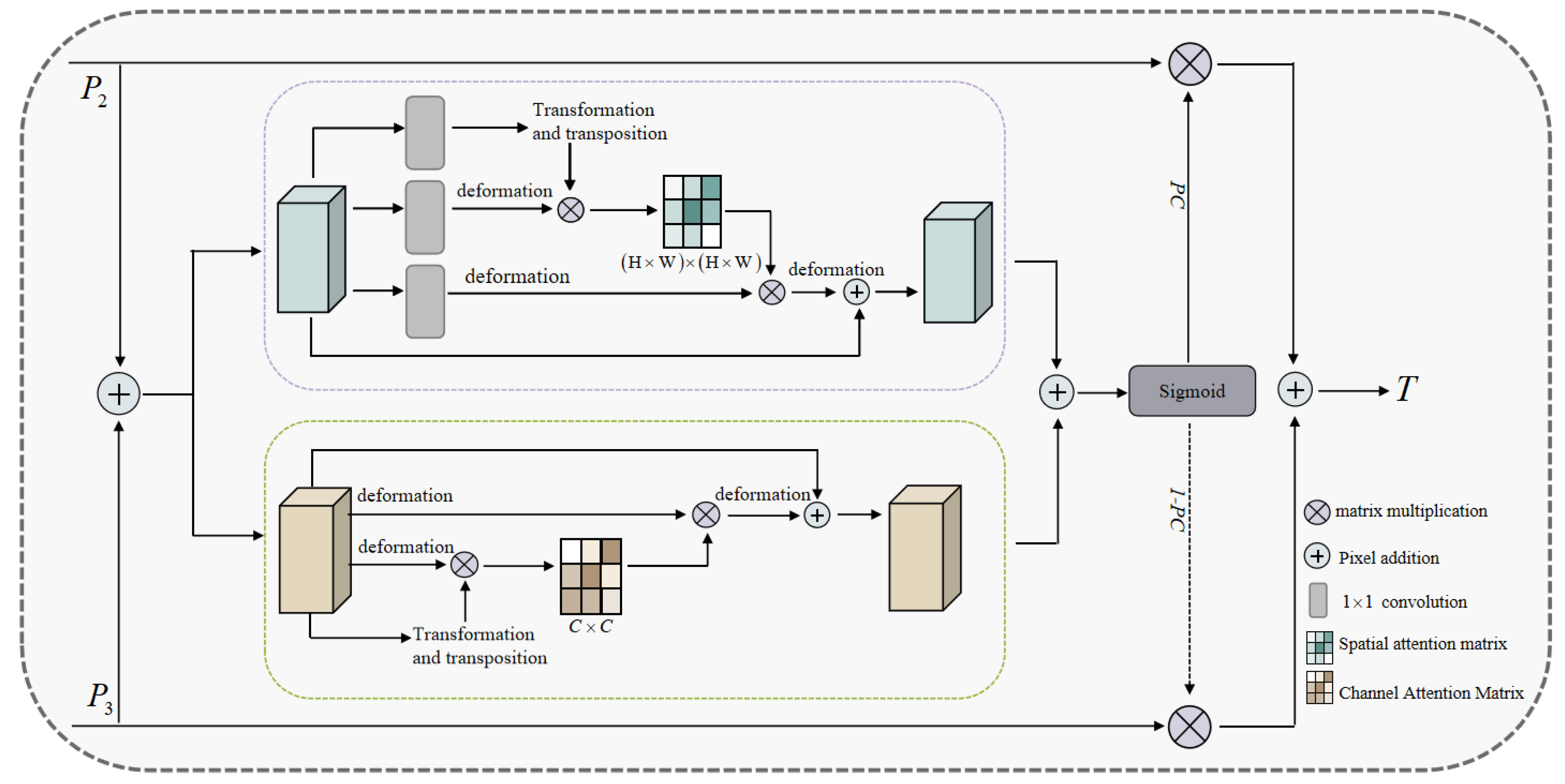
Feature fusion module based on spatial and channel attention: Spatial attention and channel attention are generally considered complementary. Spatial attention captures correlations between different positions in input features, while channel attention enhances the model’s perception of different feature channels. By combining both mechanisms, the model can better utilize spatial-channel relationships to obtain more comprehensive information representations, thereby improving the performance and generalization ability [26]. To effectively fuse the weighted features P 2 and P 3 obtained in Section 3.2, we propose a feature fusion module based on spatial and channel attention. Figure 2 illustrates the overall framework.
Given two feature maps at different scales P 2 and P 3 , based on the above multi-scale spatial and channel attention module, the fusion of attention features can be expressed as follows:
T = P C P 2 + P 3 P 2 + 1 P C P 2 + P 3 P 3
where T R C × H × W represents the fused output feature. The element-wise sum of features P 2 and P 3 is fed into both the spatial and channel attention module. P C P 2 + P 3 denotes the attention weights generated by the module. This operation enables effective weighted feature fusion through the attention mechanism [27].
(2)
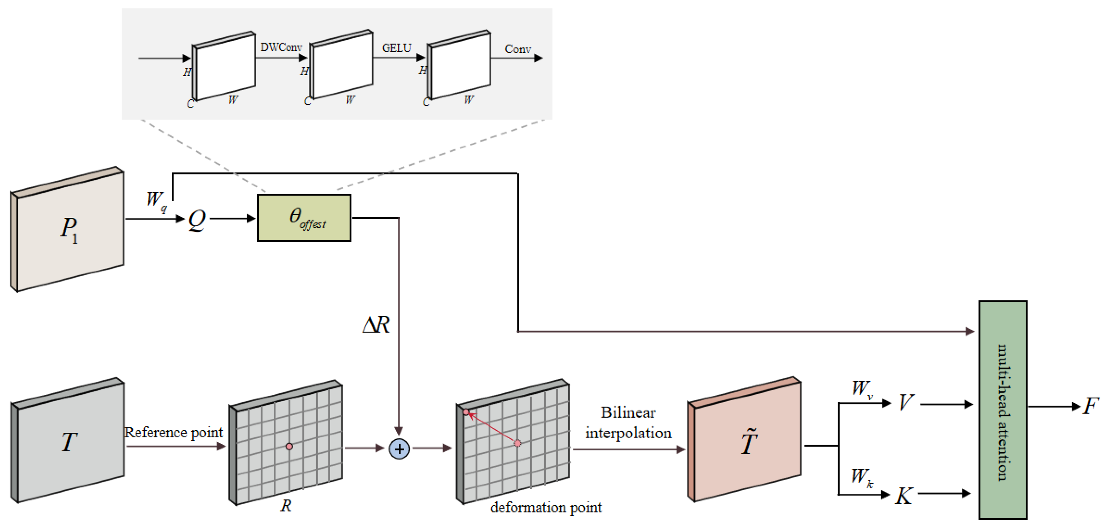
Feature fusion module based on cross-deformable attention: This paper employs a cross-deformable attention fusion module to deeply integrate the small-scale feature P 1 with the shallow feature T. Since small-scale fine features preserve finer local details, using the query from small-scale features together with the key and value from large-scale features enables better handling of cross-scale relationships. This approach simultaneously incorporates a broader global context while preserving detailed local information, thereby enhancing the model’s robustness against multi-scale variations. The complete fusion process is illustrated in Figure 3.
Specifically, the feature map P 1 R C × H × W is taken as input, and a linear transformation is applied to P 1 to obtain the query representation Q:
Q = P 1 W Q
where W Q denotes the trainable parameter matrix.
The feature map T R C × H × W is processed through a position-wise linear transformation to generate reference points R [28]. The reference points’ dimensions are H × W × 2 , with coordinate ranges spanning 0 , 0 , . . . , ( H , W ) . These coordinates are normalized to 1 , 1 . The query representation Q obtained from the transformation of P 1 is then fed into the offset network to produce displacement vectors Δ R :
Δ R = θ o f f e s t ( Q )
The deformable point is obtained by adding the computed offset Δ R to the reference point R. Based on these deformable points, this paper applies bilinear interpolation to the input feature T, using Equation (13) to generate the final adjusted feature T ˜ :
T ˜ = ϕ T ; R + Δ R
Linear transformation is applied to T ˜ to obtain K and V:
K = T ˜ W K
V = T ˜ W V
where W K and W V are trainable parameter matrices.
The output formula for multi-head attention is
T ^ = S o f t m a x Q K d + ϕ B ^ ; E V
where E denotes the relative position offset points that determine the actual sampling position offsets. The offset is predicted through network learning in deformable convolution from the input feature map. The number of relative position offset points equals that of deformable points, with each deformable point corresponding to one offset point. B ^ represents the relative position bias table adopted from the Swin transformer [29]. In this table, ϕ B ^ ; E R H W × H W is interpolated to cover all possible offset values with continuous relative displacements.
Finally, T ^ and P 1 are concatenated channel-wise to produce the final fused feature map F:
F = C o n c a t ( T ^ , P 1 )

3.4. Algorithm Implementation Process

Based on the above analysis, Algorithm 1 summarizes the specific method steps.
Algorithm 1 Hyperspectral anomaly detection algorithm.
Input: Hyperspectral image I; training epochs E
Output: Detection map L
For   e = 1 to E do
  1. Perform three different scale-central difference convolution operations 3 × 3 , 5 × 5 , and 7 × 7 on the normalized HSI to extract multi-scale spatial features S 1 , S 2 , and S 3 from different neighborhoods;
  2. Perform 3D convolution operation on the outputs of multi-scale modules S 1 , S 2 , and S 3 to obtain feature weights U 1 , U 2 , and U 3 ;
  3. Multiply U i i = 1 , 2 , 3 with S i i = 1 , 2 , 3 separately to calculate weighted features P 1 , P 2 , and P 3 ;
  4. Based on the feature fusion module of spatial and channel attention, shallow fusion is performed on features P 2 and P 3 to obtain feature T;
  5. According to the cross-deformable attention fusion module, deep fusion is performed on features T and P 1 to obtain feature F;
End For
  Perform RX calculation on the fused feature F to obtain the final detection result L.

4. Analysis and Experiment

4.1. Experimental Settings

4.1.1. Implementation

The experiments in this study were implemented using Python 3.9.21 and PyTorch 2.5.1 with CUDA 11.8 and were executed on a PC configured with an Intel Core i7-13700H CPU (2.10 GHz), 16 GB of RAM, and an NVIDIA GeForce RTX 3050 GPU with 8 GB of VRAM.
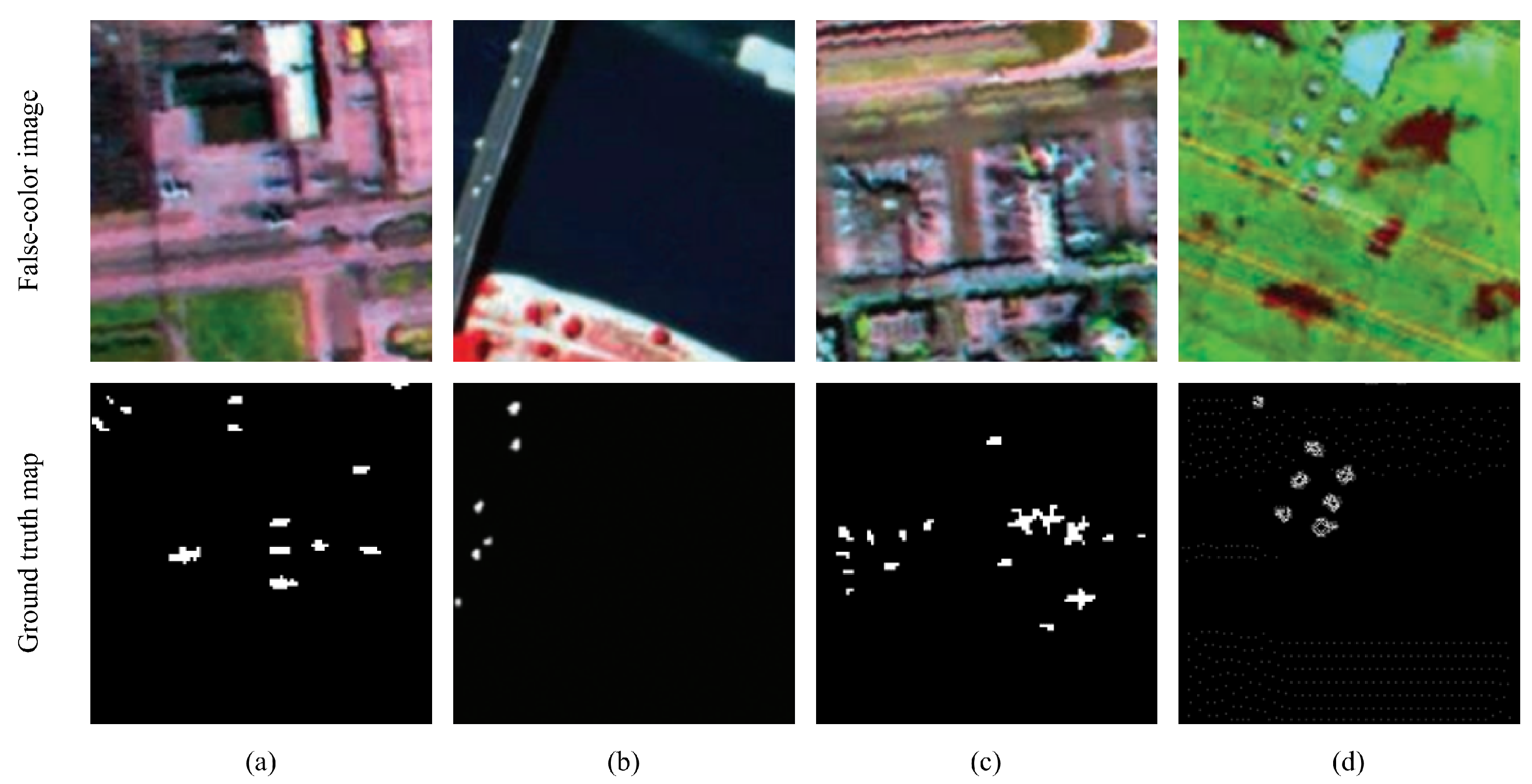
This study used the ABU-Airport datasets, Pavia Center dataset and Texas Coast datasets. Sample images and ground-truth maps of the above datasets are shown in Figure 4 [30].

4.1.2. Datasets

In this study, we used two subsets of the ABU-Airport dataset, namely Airport-1 and Airport-3. The images were acquired over Los Angeles, USA, on 9 November 2011 by the Airborne Visible/Infrared Imaging Spectrometer (AVIRIS), which was developed by the Jet Propulsion Laboratory, California Institute of Technology/NASA, Pasadena, CA, USA. The spatial resolution is 7.1 m. The selected image patches have a size of 100 × 100 pixels and contain 205 spectral bands. The aircraft in the images are regarded as anomalous targets to be detected.
The Pavia Center dataset was captured over Pavia Center in northern Italy by the Reflective Optics System Imaging Spectrometer-03 (ROSIS-03), developed by the German Aerospace Center, DLR, Oberpfaffenhofen, Germany. In our experiments, the selected image patch has a size of 100 × 100 pixels and contains 102 spectral bands. The vehicles on the bridge are labeled as anomalous targets, with 64 target pixels.
The Texas Coast dataset was captured over the Texas Coast, USA, by the Airborne Visible/Infrared Imaging Spectrometer (AVIRIS), developed by the Jet Propulsion Laboratory, California Institute of Technology/NASA, Pasadena, CA, USA. The selected image patch has a size of 100 × 100 pixels and contains 204 spectral bands. Residential buildings with varying geometries are labeled as anomalous areas.

4.2. Parameter Settings

This study employed multiple objective evaluation metrics for HSI-AD to ensure comprehensive and effective analysis of the proposed algorithm. The adopted metrics included (1) the receiver operating characteristic (ROC) curve, (2) the area under curve (AUC), and (3) the boxplot-based separability visualization.
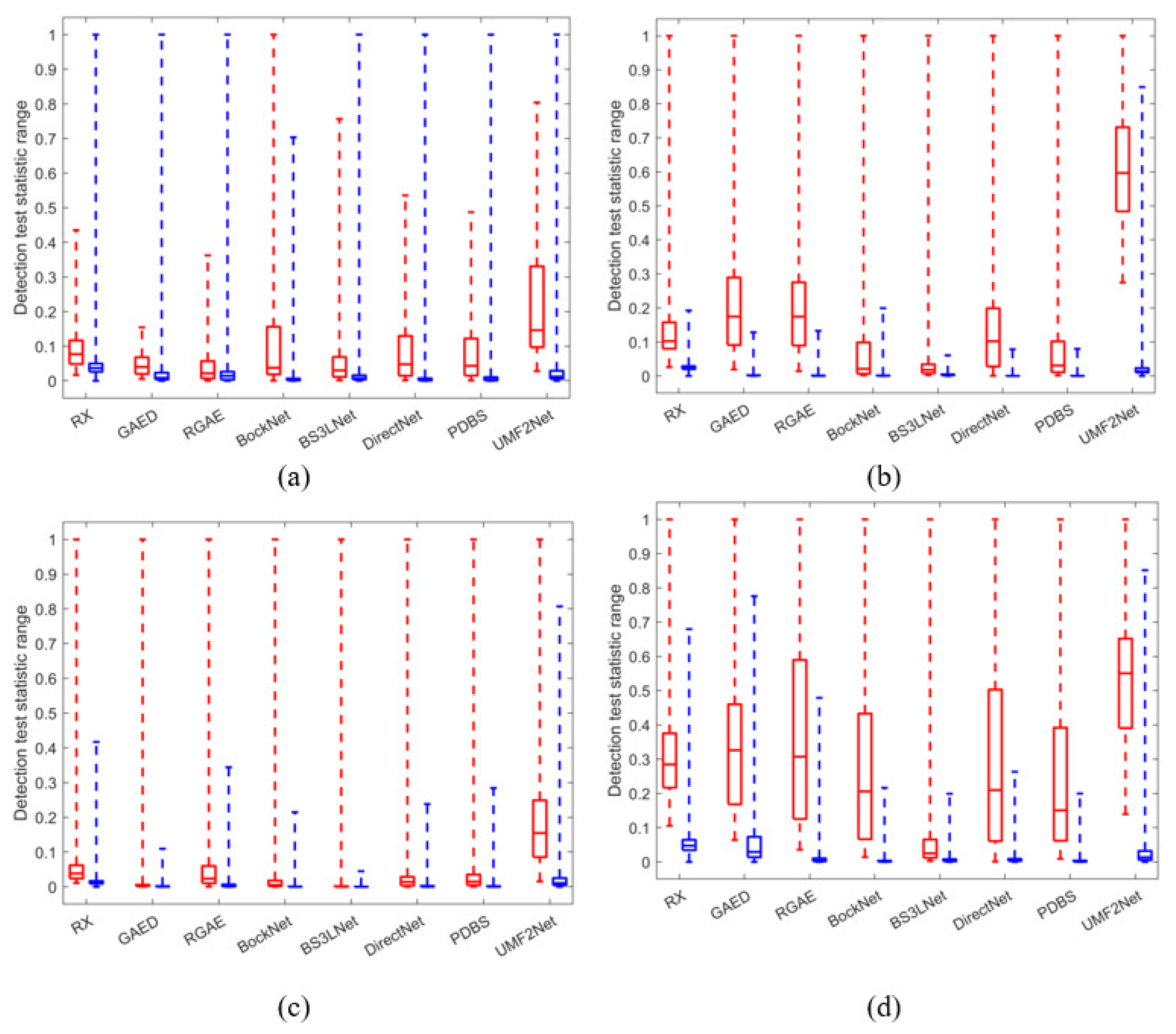
The detection performance improved as the ROC curve approached the upper-left corner, indicating both a reduced false alarm rate and an increased detection rate. The AUC measures the area enclosed by the ROC curve and both coordinate axes, serving as a standard metric for evaluating classification model performance. With a value range from 0 to 1, higher AUC values correspond to superior detection effectiveness. The visualization consists of two boxplots representing the HSI distributions of anomalous targets and background targets. The red-outlined box represents the anomaly distribution, and the blue-outlined box shows the background distribution. A larger gap between the anomaly box and the background box indicates a higher degree of separation between the anomalies and background. A shorter background box demonstrates better background suppression by the algorithm [31]:
(1)
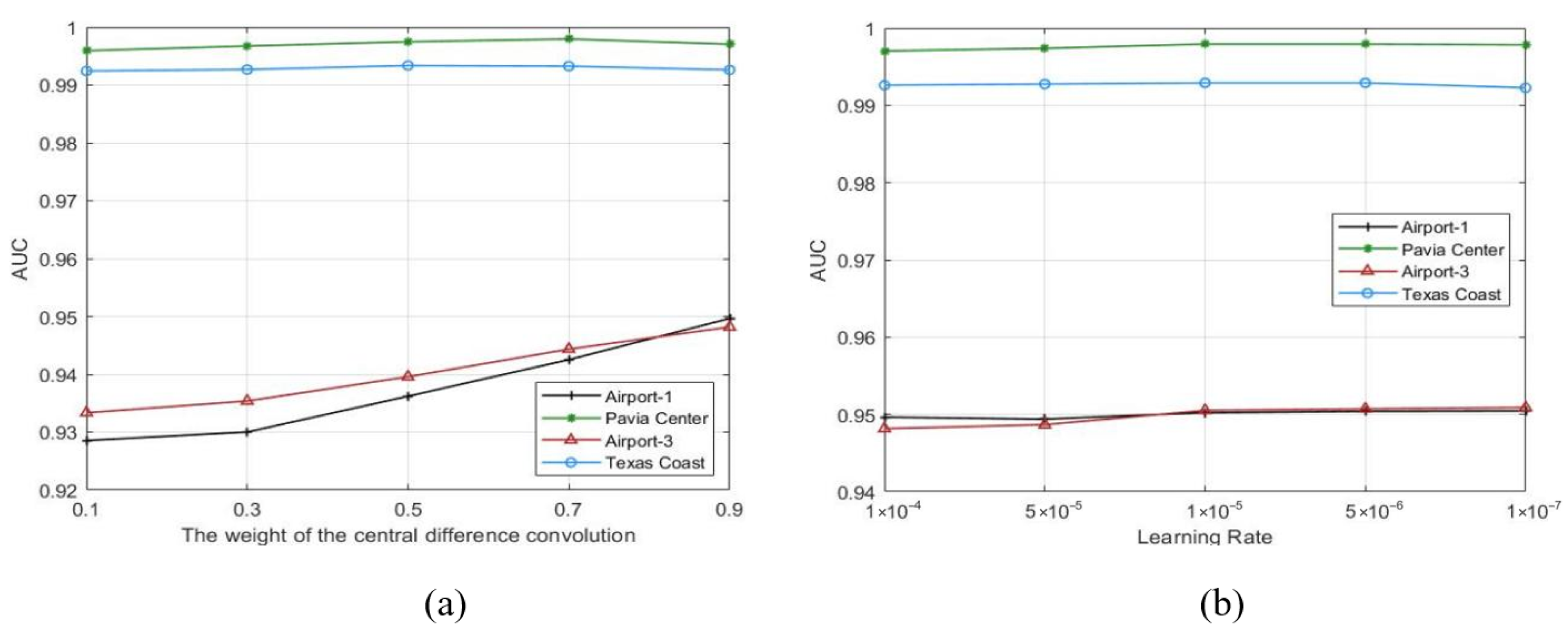
Central difference convolution parameter analysis: The parameter λ assigns different weights to the integration of ordinary convolution and differential convolution to control their impact on the output features. This balanced fusion enables the network to adaptively extract features according to task-specific requirements and data characteristics. This paper analyzes the impact of different values on the results. As shown in Figure 5a, the optimal value in the above datasets was λ = 0.9 .
(2)
Learning rate: The learning rate influences the speed of model convergence. Selecting an appropriate learning rate prevents oscillation or divergence phenomena caused by parameter updates. This paper analyzes the AD results of the experimental datasets at different learning rates. The evaluation process is illustrated in Figure 5b, and the optimal learning rate was 5 × 10 6 .

4.3. Analysis of Experimental Results

To verify the effectiveness of our proposed algorithm, we selected several AD algorithms for comparative experiments, including the RX method [9], the Guided Autoencoder (GAED) method [32], the Robust Graph Autoencoders (RGAE) method [33], the Blind-Block Reconstruction Network (BockNet) method [34], the Blind-Spot Self-Supervised Learning Network (BS3LNet) method [35], the Sliding Dual-Window-Inspired Reconstruction Network (DirectNet) method [36], and the Pixel-Shuffle Downsampling Blind-Spot Reconstruction Network (PDBS) method [37]. The parameter settings of all compared algorithms are summarized in Table 1.
(1)
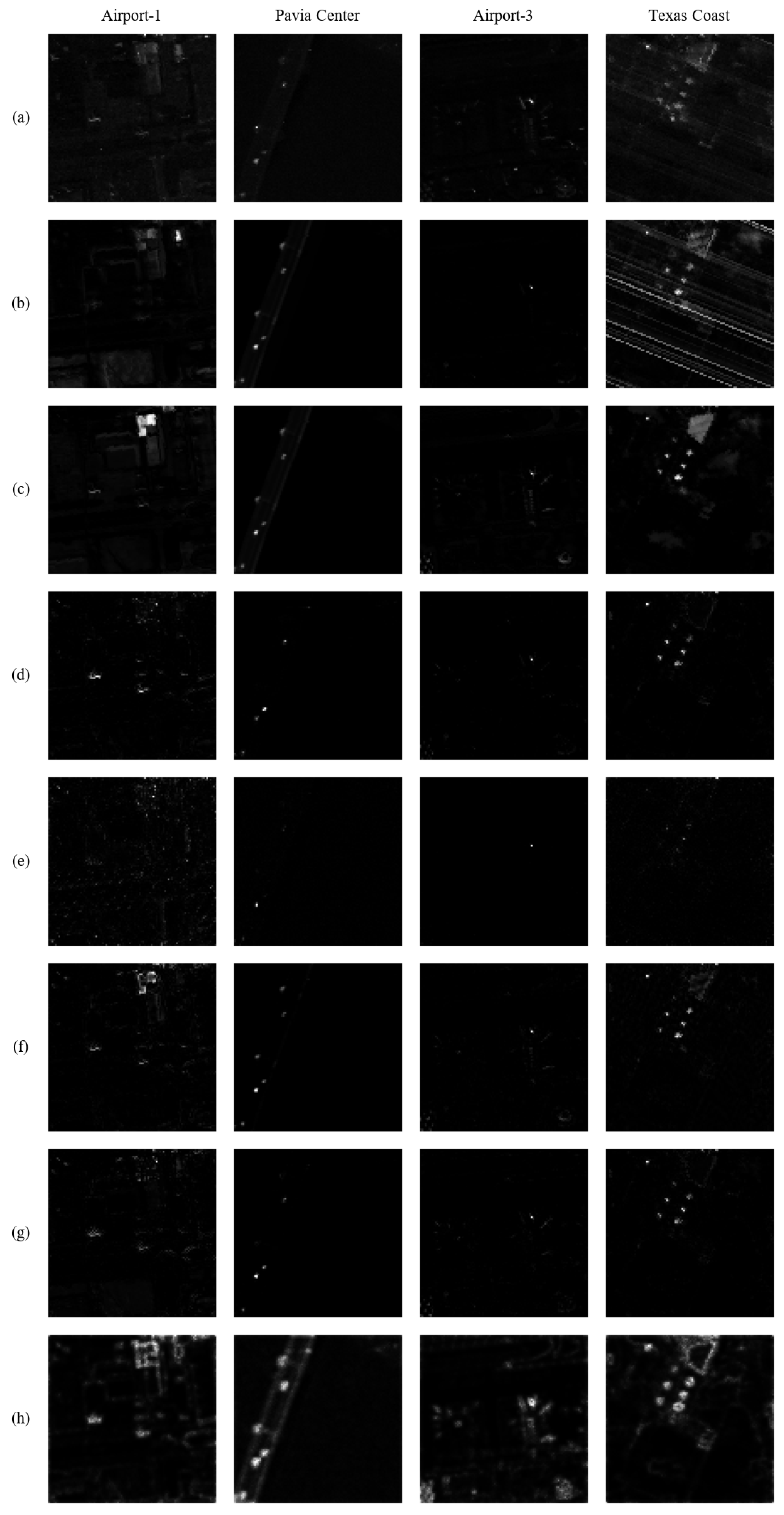
Subjective analysis: Figure 6 displays the detection results of each algorithm on the experimental datasets. Most of the compared algorithms exhibited excessive suppression. While the detection results of RGAE and GAED could capture target outlines, the lack of an effective feature weighting mechanism often led to the misclassification of high-frequency background noise as anomalous points, resulting in significant false alarms. Notably, the proposed UMF2Net algorithm exhibited a clear advantage in subjective visual analysis. It not only precisely depicted the full morphology of tiny targets, such as aircraft and vehicles, but also produced an extremely clean background, significantly enhancing the target-to-background contrast. This demonstrates that the multi-scale feature fusion strategy achieved an excellent balance between maintaining target integrity and suppressing complex background interference.
(2)
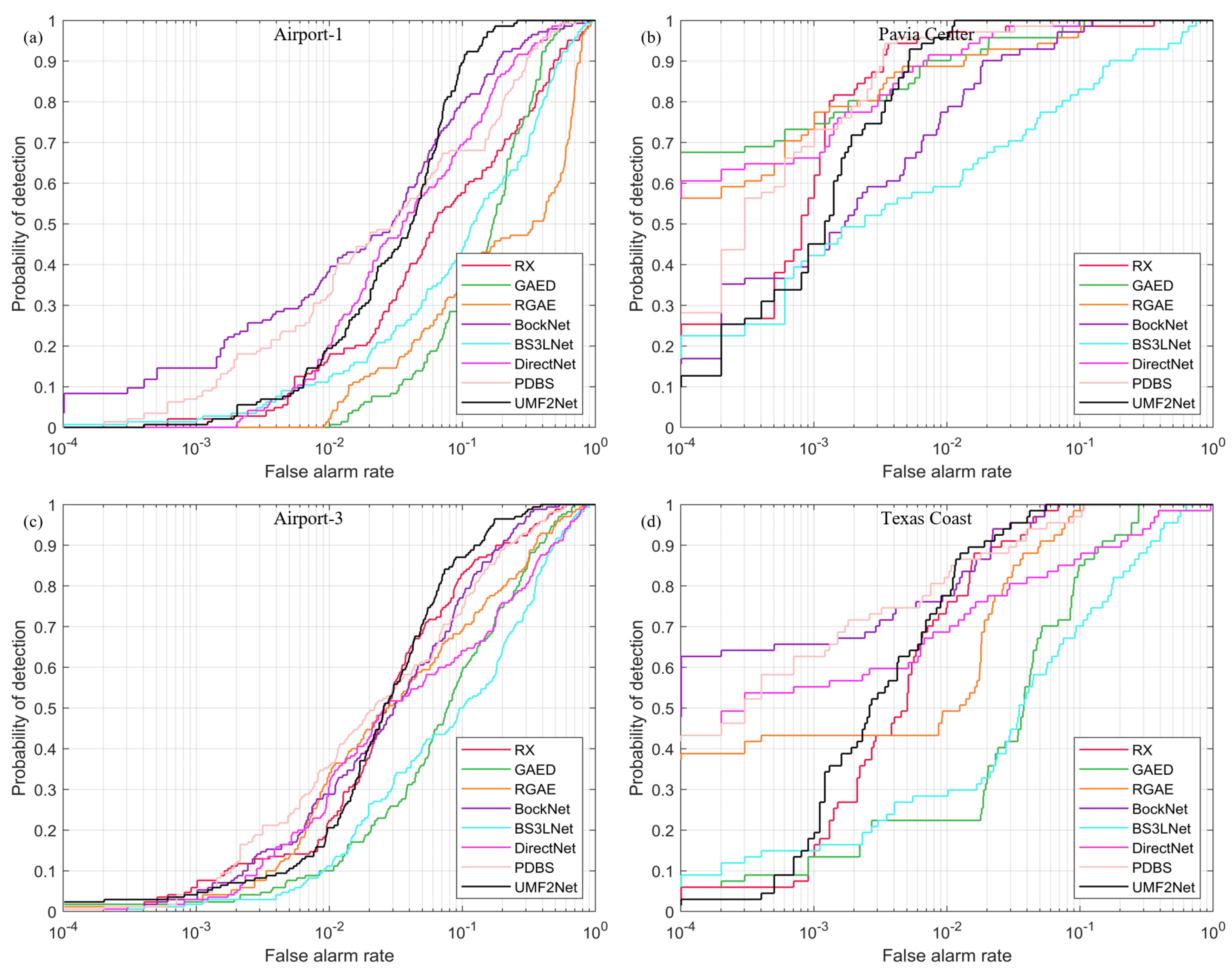
Objective analysis: Figure 7 shows the ROC curves of UMF2Net and the compared algorithms on the experimental datasets. The ROC curve of UMF2Net was generally above those of the compared methods. The black curve reached the upper-left region earlier, indicating that this algorithm can achieve higher detection rates while ensuring low false alarm rates.
Figure 8 presents the anomaly and background separation images of UMF2Net and the compared algorithms on the experimental datasets. Analysis demonstrates that UMF2Net achieved an ideal distribution across all scenarios. The median response of anomalous targets was significantly higher than that of the comparative methods, while the fluctuation range of the background pixels was compressed within an extremely small threshold. The figure shows that UMF2Net outperformed the other compared algorithms in separating the background and anomalies in various datasets while ensuring a certain background suppression rate.
Table 2 presents the AUC values of UMF2Net and the compared algorithms on the experimental datasets, with the optimal values highlighted in bold. As shown in Table 2, UMF2Net achieved the best AUC values on the Airport-1, Pavia Center, and Airport-3 datasets among all compared methods. To address the suboptimal results observed on the Texas dataset, further investigation suggests that this scenario was characterized by intricate water-land boundaries and concentrated urban infrastructure, which imposed significant non-stationarity on the spectral distribution of the background. While certain approaches like BockNet attained superior background suppression by compromising the fidelity of target detection, UMF2Net continued to deliver highly competitive detection performance. Most importantly, it struck an effective balance between achieving robust background rejection and ensuring the essential separability of anomalous targets.

4.4. Ablation Experiment

The proposed algorithm focuses on extracting three multi-scale features with a weighting mechanism. The trapezoidal deep-shallow feature fusion of the three-scale features effectively enhances the anomalies and suppresses the background. To verify the effectiveness of the weighted feature extraction module and trapezoidal depth feature fusion module, we conducted ablation experiments based on the above datasets. Table 3 presents the objective evaluation metrics, which verifies the effectiveness of the weighted feature extraction module and the trapezoidal depth feature fusion module. This demonstrates that the algorithm proposed in this paper can enhance the anomalies and suppress the background.

5. Discussion

In future research, we plan to explore the integration of the Mamba architecture into the multi-scale framework to further enhance long-range spectral dependency modeling while reducing computational overhead. Additionally, we will investigate self-adaptive receptive field techniques to improve the model’s generalization capability across satellite sensors with different spatial resolutions.

6. Conclusions

In this paper, an unsupervised multi-scale feature fusion network for HSI-AD was proposed. In HSI-AD, the size and shape of different anomalous targets may vary significantly, and the spatial distribution and interrelationship between pixels are incredibly important for image recognition. By extracting and fusing multi-scale features, the model can better handle scale changes and spatial correlations, thereby improving the accuracy of target recognition. In addition, multi-scale analysis can highlight the features of these small targets at a smaller scale to boost detection performance. This paper used central difference convolution to analyze images at different scales, capturing information on both fine- grained details and coarse structures. This process assigns different weights to features based on their contributions. The model can focus on the features that have a greater impact on the AD results while ignoring those unimportant features, and 3D convolution is used to generate feature weights for the multi-scale features. Finally, by utilizing the deep-shallow multi-scale feature fusion module, the model can better adapt to input features of different scales. By effectively fusing the rich features obtained through the above process, the model improves the detection rate for anomalies of different sizes. The source code can be found at https://github.com/WYH-yihan/UMF2Net (accessed on 1 May 2026).

Author Contributions

Methodology, software, investigation, data curation, visualization, and writing—original draft, Y.W.; conceptualization and writing—review and editing, Z.M.; writing—review and editing, H.Z.; conceptualization and writing—review and editing, C.S.; conceptualization, supervision, writing—review and editing, and funding acquisition, X.W. All authors have read and agreed to the published version of the manuscript.

Funding

This work was supported by the Key Scientific Research Project of Liaoning Provincial Education Department under Grant No. JYTZD2023101.

Data Availability Statement

The datasets used in this study are publicly available and can be accessed from the official UPV/EHU Computational Intelligence Group website at https://www.ehu.eus/ccwintco/index.php/Hyperspectral_Remote_Sensing_Scenes (accessed on 1 May 2026).

Acknowledgments

The authors would like to thank the editors and the reviewers for their valuable suggestions.

Conflicts of Interest

The authors declare no conflicts of interest.

References

  1. Cuellar, A.; Mahalanobis, A. Detection of small moving targets in cluttered infrared imagery. IEEE Trans. Aerosp. Electron. Syst. 2023, 59, 1506–1517. [Google Scholar]
  2. Hu, J.; Zheng, W.; Wang, R.; Zhao, M. A band-selected and regularized network for hyperspectral anomaly detection. IEEE Trans. Instrum. Meas. 2025, 74, 5037514. [Google Scholar] [CrossRef]
  3. Wang, R.; Hu, J. Gaussian-inspired attention mechanism for hyperspectral anomaly detection. IEEE Geosci. Remote Sens. Lett. 2025, 22, 5500705. [Google Scholar] [CrossRef]
  4. Wu, S.; Zhang, X.; Wang, G.; Chen, P.; Gu, J.; Cheng, X.; Jiao, L. VJDNet: A simple variational joint discrimination network for cross-image hyperspectral anomaly detection. Remote Sens. 2025, 17, 2438. [Google Scholar] [CrossRef]
  5. Liu, Y.; Jiang, K.; Xie, W.; Zhang, J.; Li, Y.; Fang, L. Hyperspectral anomaly detection with self-supervised anomaly prior. Neural Netw. 2025, 187, 107294. [Google Scholar] [CrossRef]
  6. Zhao, D.; Zhang, H.; Arun, P.V.; Jiao, C.; Zhou, H.; Xiang, P.; Cheng, K. SiamSTU: Hyperspectral Video Tracker based on Spectral Spatial Angle Mapping Enhancement and State Aware Template Update. Infrared Phys. Technol. 2025, 150, 105919. [Google Scholar] [CrossRef]
  7. Zhao, D.; Zhang, H.; Huang, K.; Zhu, X.; Arun, P.V.; Jiang, W.; Li, S.; Pei, X.; Zhou, H. SASU-Net: Hyperspectral video tracker based on spectral adaptive aggregation weighting and scale updating. Expert Syst. Appl. 2025, 272, 126721. [Google Scholar] [CrossRef]
  8. Jiang, W.; Zhao, D.; Wang, C.; Yu, X.; Arun, P.V.; Asano, Y.; Xiang, P.; Zhou, H. Hyperspectral video object tracking with cross-modal spectral complementary and memory prompt network. Knowl.-Based Syst. 2025, 330, 114595. [Google Scholar] [CrossRef]
  9. Reed, I.S.; Yu, X. Adaptive multiple-band CFAR detection of an optical pattern with unknown spectral distribution. IEEE Trans. Acoust. Speech Signal Process. 1990, 38, 1760–1770. [Google Scholar] [CrossRef]
  10. Ren, L.; Zhao, L.; Wang, Y. A superpixel-based dual window RX for hyperspectral anomaly detection. IEEE Geosci. Remote Sens. Lett. 2019, 17, 1233–1237. [Google Scholar] [CrossRef]
  11. Kwon, H.; Nasrabadi, N.M. Kernel RX-algorithm: A nonlinear anomaly detector for hyperspectral imagery. IEEE Trans. Geosci. Remote Sens. 2005, 43, 388–397. [Google Scholar] [CrossRef]
  12. Liu, C.; Ma, S.; Wang, H.; Wang, Y.; Li, H. A density-based cluster kernel RX algorithm for hyperspectral anomaly detection. Spectrosc. Spectr. Anal. 2019, 39, 1878–1884. [Google Scholar]
  13. Xu, Y.; Du, B.; Zhang, L.; Chang, S. A low-rank and sparse matrix decomposition-based dictionary reconstruction and anomaly extraction framework for hyperspectral anomaly detection. IEEE Geosci. Remote Sens. Lett. 2020, 17, 1248–1252. [Google Scholar] [CrossRef]
  14. Ruhan, A.; Mu, X.; He, J. Enhance tensor RPCA-based Mahalanobis distance method for hyperspectral anomaly detection. IEEE Geosci. Remote Sens. Lett. 2022, 19, 6008305. [Google Scholar]
  15. Wang, X.; Wang, Y.; Mu, Z.; Zhang, Y. UFBSM: Unmixing fusion and background sparse dictionary model for hyperspectral anomaly detection. Int. J. Remote Sens. 2024, 45, 3541–3559. [Google Scholar] [CrossRef]
  16. Jiang, K.; Xie, W.; Lei, J.; Jiang, T.; Li, Y. LREN: Low-rank embedded network for sample-free hyperspectral anomaly detection. Proc. AAAI Conf. Artif. Intell. 2021, 35, 4139–4146. [Google Scholar] [CrossRef]
  17. Wang, X.; Wang, Y.; Mu, Z.; Wang, M. FCAE-AD: Full convolutional autoencoder based on attention gate for hyperspectral anomaly detection. Remote Sens. 2023, 15, 4263. [Google Scholar] [CrossRef]
  18. Li, S.; Zhang, K.; Hao, Q.; Duan, P.; Kang, X. Hyperspectral anomaly detection with multiscale attribute and edge-preserving filters. IEEE Geosci. Remote Sens. Lett. 2018, 15, 1605–1609. [Google Scholar] [CrossRef]
  19. Liu, H.; Su, X.; Shen, X.; Zhou, X. MSNet: Self-supervised multi-scale network with enhanced separation training for hyperspectral anomaly detection. IEEE Trans. Geosci. Remote Sens. 2024, 62, 3411009. [Google Scholar] [CrossRef]
  20. Wang, Z.; Wang, X.; Tan, K.; Han, B.; Ding, J.; Liu, Z. Hyperspectral anomaly detection based on variational background inference and generative adversarial network. Pattern Recognit. 2023, 143, 109795. [Google Scholar] [CrossRef]
  21. Zhang, L.; Lin, F.; Fu, B. A joint model based on graph and deep learning for hyperspectral anomaly detection. Infrared Phys. Technol. 2024, 139, 105335. [Google Scholar] [CrossRef]
  22. Sun, X.; Zhang, Y.; Dong, Y.; Du, B. Contrastive Self-Supervised Learning-Based Background Reconstruction for Hyperspectral Anomaly Detection. IEEE Trans. Geosci. Remote Sens. 2025, 63, 5504312. [Google Scholar] [CrossRef]
  23. Chen, W.; Zhi, X.; Jiang, S.; Huang, Y.; Han, Q.; Zhang, W. DWSDiff: Dual-Window Spectral Diffusion for Hyperspectral Anomaly Detection. IEEE Trans. Geosci. Remote Sens. 2025, 63, 5504617. [Google Scholar] [CrossRef]
  24. Sun, D.; Zhong, S.; Gong, C. Mamba-Enhanced Background Suppression Diffusion Model for Hyperspectral Anomaly Detection. IEEE J. Sel. Top. Appl. Earth Obs. Remote Sens. 2026, 19, 5168–5182. [Google Scholar] [CrossRef]
  25. Wang, X.; Wang, L.; Vizziello, A.; Gamba, P. Hyperspectral anomaly detection based on multiscale central difference convolution network. IEEE Geosci. Remote Sens. Lett. 2023, 20, 3305814. [Google Scholar] [CrossRef]
  26. Fu, J.; Liu, J.; Tian, H.; Li, Y.; Bao, Y.; Fang, Z.; Lu, H. Dual attention network for scene segmentation. In Proceedings of the IEEE/CVF Conference on Computer Vision and Pattern Recognition (CVPR), Long Beach, CA, USA, 16–21 June 2019; pp. 3146–3154. [Google Scholar]
  27. Dai, Y.; Gieseke, F.; Oehmcke, S.; Wu, Y.; Barnard, K. Attentional feature fusion. In Proceedings of the IEEE/CVF Winter Conference on Applications of Computer Vision (WACV), Virtual, 5–9 January 2021; pp. 3560–3569. [Google Scholar]
  28. Xia, Z.; Pan, X.; Song, S.; Li, L.E.; Huang, G. Vision transformer with deformable attention. In Proceedings of the IEEE/CVF Conference on Computer Vision and Pattern Recognition (CVPR), New Orleans, LA, USA, 18–24 June 2022; pp. 4794–4803. [Google Scholar]
  29. Liu, Z.; Lin, Y.; Cao, Y.; Hu, H.; Wei, Y.; Zhang, Z.; Lin, S.; Guo, B. Swin transformer: Hierarchical vision transformer using shifted windows. In Proceedings of the IEEE/CVF International Conference on Computer Vision (ICCV), Montreal, QC, Canada, 10–17 October 2021; pp. 9992–10002. [Google Scholar]
  30. Mu, Z.; Wang, M.; Wang, Y.; Song, R.; Wang, X. SI2FM: SID isolation double forest model for hyperspectral anomaly detection. Remote Sens. 2023, 15, 612. [Google Scholar] [CrossRef]
  31. Mu, Z.; Wang, Y.; Zhang, Y.; Song, C.; Wang, X. MPDA: Multivariate probability distribution autoencoder for hyperspectral anomaly detection. IEEE Trans. Geosci. Remote Sens. 2024, 62, 3496355. [Google Scholar] [CrossRef]
  32. Xiang, P.; Ali, S.; Jung, S.K.; Zhou, H. Hyperspectral anomaly detection with guided autoencoder. IEEE Trans. Geosci. Remote Sens. 2022, 60, 5538818. [Google Scholar] [CrossRef]
  33. Fan, G.; Ma, Y.; Mei, X.; Fan, F.; Huang, J.; Ma, J. Hyperspectral anomaly detection with robust graph autoencoders. IEEE Trans. Geosci. Remote Sens. 2022, 60, 5511314. [Google Scholar] [CrossRef]
  34. Wang, D.; Zhuang, L.; Gao, L.; Sun, X.; Huang, M.; Plaza, A. BockNet: Blind-block reconstruction network with a guard window for hyperspectral anomaly detection. IEEE Trans. Geosci. Remote Sens. 2023, 61, 5531916. [Google Scholar] [CrossRef]
  35. Gao, L.; Wang, D.; Zhuang, L.; Sun, X.; Huang, M.; Plaza, A. BS3LNet: A new blind-spot self-supervised learning network for hyperspectral anomaly detection. IEEE Trans. Geosci. Remote Sens. 2023, 61, 5504218. [Google Scholar] [CrossRef]
  36. Wang, D.; Zhuang, L.; Gao, L.; Sun, X.; Zhao, X.; Plaza, A. Sliding dual-window-inspired reconstruction network for hyperspectral anomaly detection. IEEE Trans. Geosci. Remote Sens. 2024, 62, 5504115. [Google Scholar] [CrossRef]
  37. Wang, D.; Zhuang, L.; Gao, L.; Sun, X.; Huang, M.; Plaza, A.J. PDBSNet: Pixel-shuffle downsampling blind-spot reconstruction network for hyperspectral anomaly detection. IEEE Trans. Geosci. Remote Sens. 2023, 61, 5511914. [Google Scholar] [CrossRef]
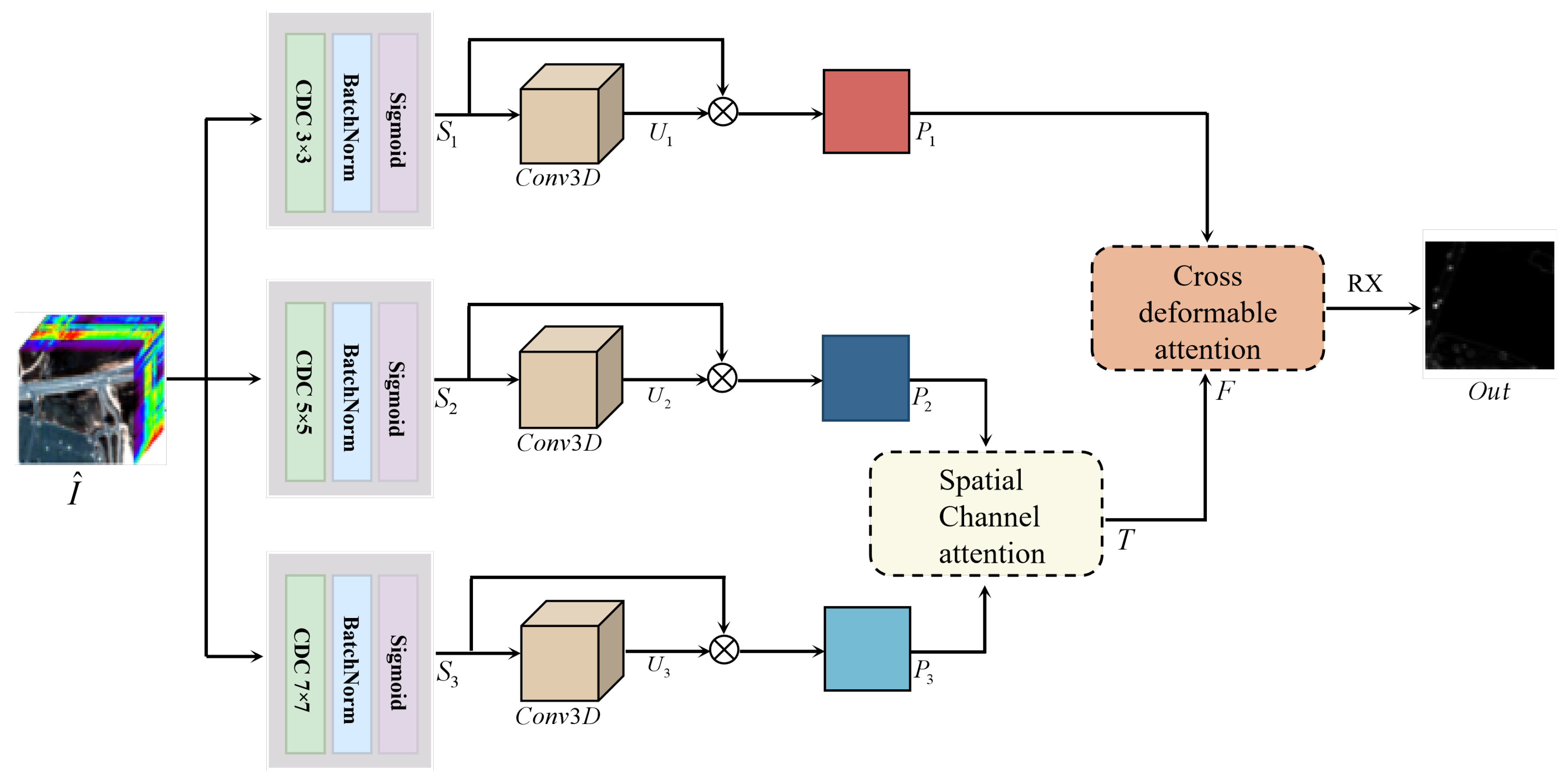
Figure 1. Schematic diagram of the overall network structure. The symbol “⊗” denotes element-wise multiplication for feature weighting, and different colors indicate different feature branches or processing stages.
Remotesensing 18 01554 g001
Figure 2. Schematic diagram of spatial and channel attention fusion module.
Remotesensing 18 01554 g002
Figure 3. Schematic diagram of the cross-deformable attention module. ⊕ denotes element-wise addition, and different colors distinguish different functional modules.
Remotesensing 18 01554 g003
Figure 4. False-color images and ground-truth maps. (a) Airport-1. (b) Pavia Center. (c) Airport-3. (d) Texas Coast.
Remotesensing 18 01554 g004
Figure 5. Comparison of model performance under different parameter values. (a) Central difference convolution parameter analysis. (b) Learning rate.
Remotesensing 18 01554 g005
Figure 6. Detection results of various algorithms. (a) RX. (b) GAED. (c) RGAE. (d) BockNet. (e) BS3LNet. (f) DirectNet. (g) PDBSNet. (h) UMF2Net.
Remotesensing 18 01554 g006
Figure 7. ROC curves of different algorithms on various datasets. (a) Airport-1. (b) Pavia Center. (c) Airport-3. (d) Texas Coast.
Remotesensing 18 01554 g007
Figure 8. Box separation graphs of different algorithms on different datasets. The red boxes represent anomaly regions, and the blue boxes represent background regions. (a) Airport-1. (b) Pavia Center. (c) Airport-3. (d) Texas Coast.
Remotesensing 18 01554 g008
Table 1. Comparison algorithm parameter settings.
AlgorithmParameter Settings
RX
GAED c = 7 , l a = 0.1 , β = 10 , r i t e r = 300
RGAE λ = 0.01 , S = 150 , n _ h i d = 100
BockNet B s = 15
BS3LNet P s = 19 , R c = 0.9 , W s = 5
DirectNet W i n = 3 , W o u t = 19
PDBSNet f a c t o r _ t r a i n = 2 , f a c t o r _ t e s t = 2
Table 2. AUC values of different algorithms on various datasets.
DatasetRXGAEDRGAEBockNetBS3LNetDirectNetPDBSUMF2Net
Airport-10.82210.80220.63870.92820.78490.90850.89780.9504
Pavia Center0.99340.99480.99270.98960.92970.99640.99770.9979
Airport-30.92880.85870.88740.93140.81220.85440.92250.9508
Texas Coast0.99070.94080.98230.99390.89580.94840.99100.9929
Note: Bold values indicate the best performance for each dataset.
Table 3. Analysis of ablation experiments.
ModuleAirport-1PaviaAirport-3Texas
None0.91430.99470.91490.9832
Weighted feature extraction0.93070.99540.93360.9849
Weighted + shallow fusion0.94160.99640.94220.9885
Full UMF2Net0.95040.99790.95080.9929
Note: Bold values indicate the best performance for each dataset.
Disclaimer/Publisher’s Note: The statements, opinions and data contained in all publications are solely those of the individual author(s) and contributor(s) and not of MDPI and/or the editor(s). MDPI and/or the editor(s) disclaim responsibility for any injury to people or property resulting from any ideas, methods, instructions or products referred to in the content.