A Spatio-Temporal Machine Learning Framework for High-Accuracy Thermal Mapping of Dynamic Coastal Waters Using UAV Imagery

Highlights

What are the main findings?

• An MLP model fusing spatio-temporal features achieves high-accuracy UAV SST retrieval (R² = 0.9980, MAE = 0.1523 °C).
• Yaw angle clustering effectively eliminates geometric distortions in mosaicking texture-less sea surface images.
• The non-linear relationship between UAV-retrieved and actual temperatures exhibits significant seasonal and tidal variations.
• High-resolution SST maps reveal the specific diffusion patterns of nuclear power plant thermal plumes under varying tidal dynamics.

What are the implications of the main findings?

• Incorporating environmental contexts (tide, season, coordinates) fundamentally improves the accuracy and robustness of UAV thermal remote sensing models.
• The automated image filtering strategy provides a geometrically reliable and efficient solution for mapping vast aquatic environments using UAV swarms.
• Integrating multi-UAV observation and machine learning establishes a rapid, cross-seasonal paradigm for the precise environmental regulation of coastal nuclear power plants.

Abstract

Unmanned aerial vehicle (UAV) thermal imagery is a powerful tool for monitoring coastal waters, but achieving high-accuracy temperature retrieval remains a major challenge due to complex, non-linear biases introduced by dynamic environmental conditions. This study presents a novel spatio-temporal machine learning framework to overcome this limitation. The core innovation is a multi-layer perceptron (MLP) model that decouples sensor readings from environmental effects by integrating UAV-retrieved temperatures with crucial contextual features: geographical coordinates (spatial) and tidal status (temporal). Applied to the challenging scenario of a nuclear power plant’s thermal plume, the framework demonstrated exceptional performance. On the test set, the model achieved a coefficient of determination (R²) of 0.998 and a mean absolute error (MAE) of only 0.15 °C, significantly outperforming traditional regression approaches. Ultimately, this method successfully generated high-resolution, high-accuracy sea surface temperature (SST) maps under 24 distinct tidal conditions spanning both summer and winter seasons. This work provides a robust and transferable framework for the quantitative thermal mapping of any complex and dynamic aquatic environment using UAVs.

1. Introduction

In response to the global warming caused by greenhouse gas emissions, governments worldwide have recently strengthened their ambitions and commitments to achieving net-zero emissions, leading to a continuously rising global demand for clean and sustainable energy [1,2,3,4]. As a low-carbon energy source, nuclear power is regarded as a vital means to mitigate greenhouse gas emissions and combat climate change, playing a significant role in promoting global economic and social development [5,6,7,8]. To ensure operational safety, nuclear power plants require large volumes of water for reactor cooling, and the resulting thermal discharge continuously enters adjacent sea areas, causing a significant increase in local sea surface temperature (SST) [9,10]. The extent and intensity of this thermal diffusion are complexly regulated not only by the discharge flow rate and duration but also by marine environmental factors such as tidal dynamics, seabed topography, and ocean currents [11,12,13]. The thermal discharge from nuclear power plants may lead to elevated water temperatures, causing damage to marine and lacustrine ecosystems and potentially having adverse effects on fisheries, thereby drawing significant attention from environmental organizations and the scientific community. To precisely assess the potential impacts of thermal discharge on marine ecology, there is an urgent need for advanced temperature measurement technologies to achieve spatiotemporal dynamic monitoring of near-shore waters [14,15].

The construction of nuclear power plants is rapidly expanding globally, yet there is currently a lack of dynamic monitoring for the warming effects of their thermal discharges, making it difficult for governments to accurately grasp the global positioning of their national thermal discharge situations [16,17]. Various methods for monitoring and predicting thermal discharge exist, including in-situ measurements, satellite remote sensing, and UAV monitoring, all of which have played a positive role in monitoring thermal discharges from coastal nuclear power plants. Early monitoring of thermal discharge primarily relied on in-situ measurements, typically using thermometers for direct measurement [18]. Although this method is simple, it can only acquire single-layer water temperature data. However, due to its limited monitoring scope, in-situ measurement cannot meet the demands of large-scale thermal discharge assessment and is therefore rarely used alone for this purpose [19].

Satellite remote sensing utilizes satellites to detect the ocean, with common detection techniques including infrared and microwave remote sensing [20,21,22]. Both thermal infrared and microwave remote sensing of water surface temperature are based on the principle that all objects radiate electromagnetic waves in the infrared and microwave bands, with the radiation intensity being positively correlated with the object’s temperature [23]. Wang et al. used a decade of Landsat data from 2013–2022 to conduct a comparative analysis of the spatiotemporal characteristics of thermal discharge from nuclear power plants in different countries [17]. Based on Landsat satellite data, Nie et al. systematically analyzed the change characteristics of SST over a 20-year period before and after the operation of the Tianwan Nuclear Power Plant [24]. Zoran et al. used Landsat TM, MODIS, and ASTER satellite imagery to monitor the Cernavodă Nuclear Power Plant, analyzing the relationship between seasonal variations in thermal discharge and water layer stratification [25]. Huang et al. conducted remote sensing monitoring of thermal discharge from four coastal nuclear power plants in China using SDGSAT-1 imagery, whose high spatial resolution enabled clearer boundary identification [26]. Wei et al. combined Landsat imagery with deep learning techniques to achieve long-term monitoring of thermal discharge from nuclear power plants globally [27]. However, conventional satellite series like Landsat and MODIS, despite their large fields of view and wide monitoring ranges, are hampered by long revisit times, relatively coarse spatial resolution, and the influence of cloud and rain, making it difficult for them to monitor short-term temperature changes in the near-shore areas of nuclear power plants.

With the decreasing cost of UAVs and the miniaturization of thermal infrared instruments, the advantages of UAVs in thermal discharge monitoring have become increasingly prominent. In recent years, scholars have begun to explore the use of aerial remote sensing to monitor the spatiotemporal distribution of thermal discharge [28]. Compared to traditional methods, monitoring thermal discharge distribution using aerial surveillance offers the advantages of low cost and high timeliness, and it can also identify multiple heat sources simultaneously, determining the origin and destination of high-temperature water bodies. For instance, Shi used a UAV to monitor real-time changes in the sea temperature field during summer spring and neap tides, analyzing the distribution of thermal discharge under different tidal conditions based on temperature rise envelope data. Wang et al. studied the thermal discharge of the Hongyanhe Nuclear Power Plant using a UAV and accurately obtained information on its diffusion [29]. HsingYu et al. used a rotary-wing UAV to study sea temperature distribution, identifying the scope of thermal discharge diffusion and its influencing factors [30]. These studies demonstrate that UAVs can effectively compensate for the deficiencies of existing monitoring techniques, offering advantages of high efficiency, convenience, and high accuracy. However, these studies have either ignored or underestimated the impact of different images on temperature retrieval during data registration, which can introduce certain errors.

However, the operational application of UAV thermal remote sensing for near-shore monitoring still faces two major challenges. First, constructing geometrically reliable orthoimages over vast, textureless water surfaces using standard Structure from Motion (SfM) algorithms often fails, severely hindering accurate spatial analysis. Second, the high-accuracy retrieval of true, absolute SST from raw thermal infrared imagery remains a core challenge. The relationship between the UAV-retrieved temperature and the actual sea temperature is influenced by the complex coupling of sensor-intrinsic errors, spatial location, and instantaneous marine hydrodynamics. Furthermore, current UAV-based monitoring predominantly focuses on single-season observations, lacking comprehensive validation across different climatic backgrounds (e.g., summer vs. winter). Most existing studies rely on traditional linear or polynomial regression for temperature correction. Due to their simple structures, these models struggle to fit this non-linear relationship, resulting in limited accuracy and significant performance fluctuations under different seasonal and environmental conditions.

To address these key scientific problems, this study, taking the Fuqing Nuclear Power Plant as a case study, proposes a novel paradigm for the high-accuracy retrieval of near-shore SST based on machine learning. We developed a Multi-Layer Perceptron (MLP) model to precisely correct the initial temperatures retrieved from the UAV. The core innovation of this model is the fusion of multi-dimensional feature information: it creatively introduces key contextual factors, including geospatial coordinates, tidal dynamics, and seasonal backgrounds, alongside the direct UAV observations. By learning the complex relationship between these features and the true temperature, the model can adaptively capture and correct systematic biases across varying climatic and hydrodynamic conditions.

The main contributions and innovations of this paper are as follows:

• An environmentally-aware machine learning temperature correction model is proposed. By fusing sensor data with multi-dimensional spatiotemporal features (including spatial coordinates, tidal status, and season), this model effectively solves the non-linear correction problem. Its exceptional accuracy and robustness have been systematically validated across 24 distinct tidal conditions spanning both summer and winter seasons, significantly outperforming traditional regression methods.
• An optimization strategy for UAV image mosaicking applicable to wide-area, textureless sea surfaces is developed. To ensure an accurate spatial assessment of the thermal discharge, we propose an automatic image filtering method based on yaw angle clustering. This method effectively overcomes the technical bottleneck of severe geometric distortion during the mosaicking process over water, providing a highly reliable base image for accurately delineating the thermal plume.
• A complete, cross-seasonal, and high-precision technical workflow for UAV thermal remote sensing is established. This framework provides a proven, rapid-response solution for the fine-scale, periodic regulation of the dynamic near-shore thermal environments of nuclear power plants and similar critical coastal infrastructures.

The remainder of this paper is structured as follows: Section 2 introduces the study area and the detailed data acquisition scheme; Section 3 describes the data pre-processing, MLP model construction, and evaluation methods; Section 4 presents the model’s accuracy validation results and the final retrieved retrieved spatiotemporal distribution maps of the thermal discharge; Section 5 presents the conclusions of this study.

2. Study Site and Datasets

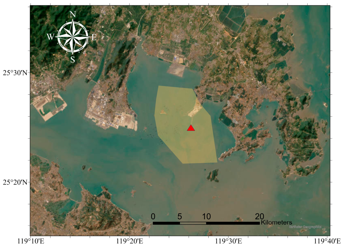
As shown in Figure 1, the observation area of this study is located in Xinghua Bay, adjacent to the Fuqing Nuclear Power Plant in Fujian Province, China. The plant is situated on a wedge-shaped peninsula surrounded by the sea on its southeast, southwest, and northwest sides. The region belongs to a subtropical monsoon climate zone, characterized by warm temperatures and abundant rainfall, with an annual average temperature of approximately 19.7 °C. The hydrodynamic environment of the study area is complex and highly dynamic, dominated by regular semidiurnal tides. The tidal currents are predominantly reciprocating, mainly controlled by the Xinghua and Nanri waterways, with the average flood tide duration being shorter than the average ebb tide duration. These unique geographical and hydrological conditions significantly influence the dispersion and dilution of the thermal plume, providing an ideal natural laboratory for investigating the spatiotemporal evolution of thermal discharges under varying seasonal and tidal dynamics.

To construct and rigorously validate a cross-seasonal, high-accuracy temperature retrieval model, this study designed a coordinated air-ground synchronous observation scheme. Comprehensive field experiments were conducted during both Summer (July to August 2023) and Winter (December 2023 to January 2024). This scheme integrates multi-UAV thermal infrared aerial remote sensing with simultaneous ship-borne in-situ sea surface temperature (SST) measurements. The primary aerial data acquisition platform was the DJI M3T UAV (DJI, Shenzhen, China), which integrates a high-resolution thermal infrared camera (640 × 512 pixels), a high-precision RTK-GNSS module, and a three-axis stabilized gimbal. A major operational challenge was the sheer scale of the experimental area, which exceeds 100 square kilometers. Given the rapid dynamic changes in SST, it was imperative to complete a full-coverage data acquisition within a strict 1-h time window. Constrained by the limited battery endurance of a single UAV, covering this entire area sequentially would take over ten hours and violate the synchronous observation requirement. To overcome this, a multi-UAV coordinated operation scheme was innovatively designed. The vast experimental area was pre-gridded into ten sub-regions. Taking into account flight altitude (approximately 500 m), image overlap requirements, boat deployment for takeoff and landing, and field personnel allocation, a swarm of ten UAVs was dispatched to conduct data acquisition simultaneously across all sub-regions.

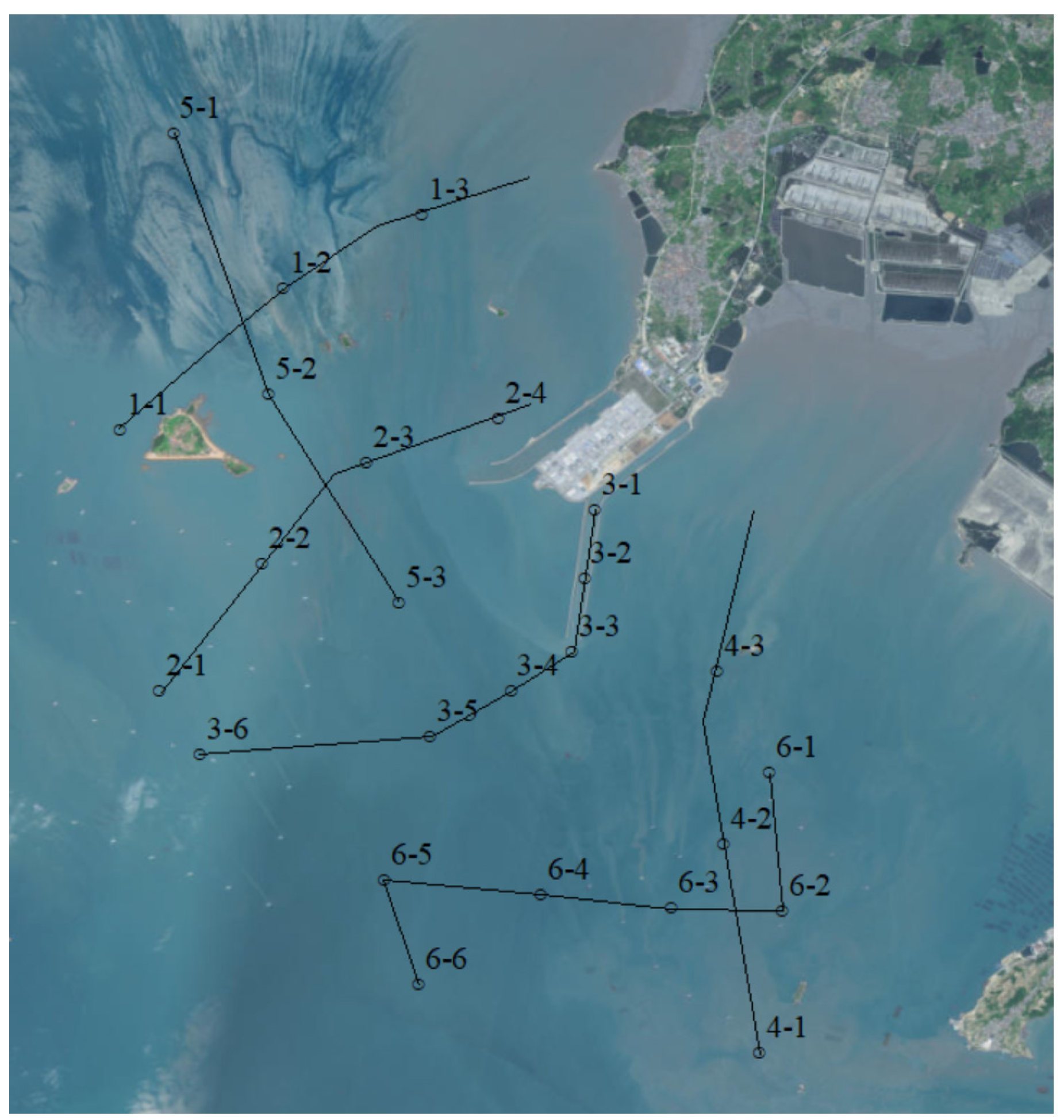
To achieve precise absolute temperature calibration and provide ground truth for the machine learning model, ship-borne transect measurements of SST were conducted strictly synchronously with the UAV aerial surveys. As shown in Figure 2, a total of 6 synchronous observation transects were established within the study area. The observation system employed a combined mode: a Differential Global Positioning System (DGPS) was used for high-precision positioning (CGCS2000 coordinate system), and a CTD (Conductivity, Temperature, Depth) instrument was used for highly sensitive temperature measurement. To comprehensively capture temperature variations under varying hydrodynamic contexts, the observation periods in both summer and winter were meticulously selected to cover three typical tidal types (spring, intermediate, and neap) and four key tidal states (flood slack, maximum flood, ebb slack, and maximum ebb). The in-situ measurements for each tidal state were kept synchronous or quasi-synchronous with the UAV’s aerial observations, ensuring that the measurement tasks for all transects were completed within 1 h. Regarding the temporal resolution, we employed an event-based irregular sampling strategy driven by tidal phases. Rather than continuous time-series monitoring, the UAV swarm captured all imagery across the entire target area within a strict 1-h window for each specific tidal state, providing a quasi-synchronous temporal snapshot. Specifically, the summer observation campaigns were conducted between 4 and 9 August 2023 (spring tides on 4–5 August, intermediate tides on 7 August, and neap tides on 9 August). The winter campaigns were conducted between 6 and 14 December 2023 (neap tides on 6 December, intermediate tides on 10 December, and spring tides on 14 December). On each observation day, the four key tidal states (maximum flood, flood slack, maximum ebb, and ebb slack) were sequentially captured, with each flight mission strictly controlled within a one-hour duration to ensure temporal consistency.

During field operations, the CTD instrument was rigidly mounted on a pole attached to the side of the boat hull, with the probe positioned at a depth of approximately 0.5 m below the water surface, adjustable based on real-time wave conditions. The CTD was configured to sample at a frequency of 1 Hz with a measurement accuracy of no less than 0.1 °C. Concurrently, planar positions were recorded at 1-s intervals using HYPACK professional navigation software (version 2009a). Throughout the measurement process, strict time synchronization control between the DGPS positioning data and the CTD temperature data was maintained via the HYPACK software, which was crucial for ensuring the accuracy of subsequent data fusion. After each measurement task, the spatial and thermal data collected by HYPACK and the CTD were precisely merged based on their synchronous timestamps, ultimately generating the high-fidelity ground truth dataset used for subsequent model analysis.

3. Methodology

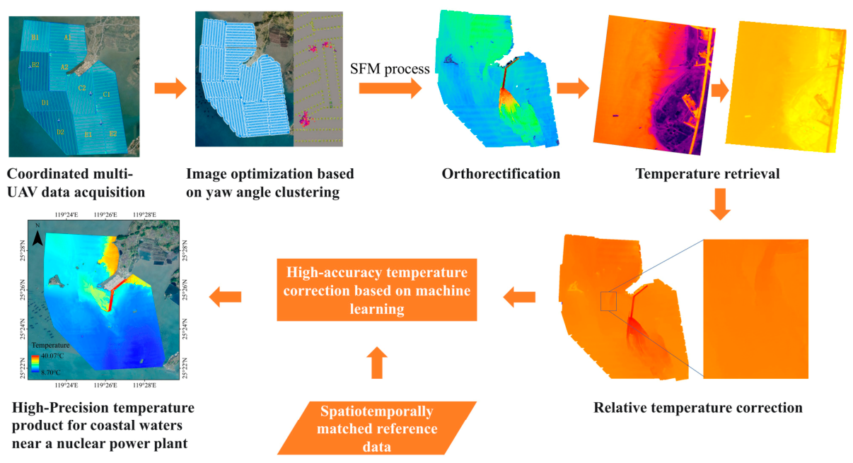
The technical core of this study is to establish a complete workflow, from raw UAV imagery to high-accuracy absolute sea surface temperature maps, for the special and complex monitoring scenario of near-shore areas of nuclear power plants. As shown in Figure 3, this workflow first employs an image optimization strategy based on yaw angle clustering to filter and mosaic the images collected by the UAV over wide-area, textureless water surfaces, in order to generate a geometrically highly reliable orthoimage. Subsequently, the relative UAV temperature is retrieved based on a radiative transfer algorithm. Finally, we developed a MLP that fuses spatial and environmental features to replace traditional linear regression algorithms, performing high-accuracy non-linear correction on the relative temperature to ultimately generate the absolute temperature product.

3.1. UAV Image Pre-Processing and Initial Temperature Retrieval

To accurately depict the wide-area spatial morphology of the nuclear power plant’s thermal plume, it is first necessary to mosaic thousands of individual UAV images into a single orthoimage with a high degree of geometric uniformity. However, on the vast and extremely texture-scarce ocean surface, the traditional Structure from Motion (SfM) algorithm is completely ineffective due to its inability to extract and match feature points. To this end, we have developed an optimization strategy that combines high-precision direct georeferencing with an innovative image filtering method.

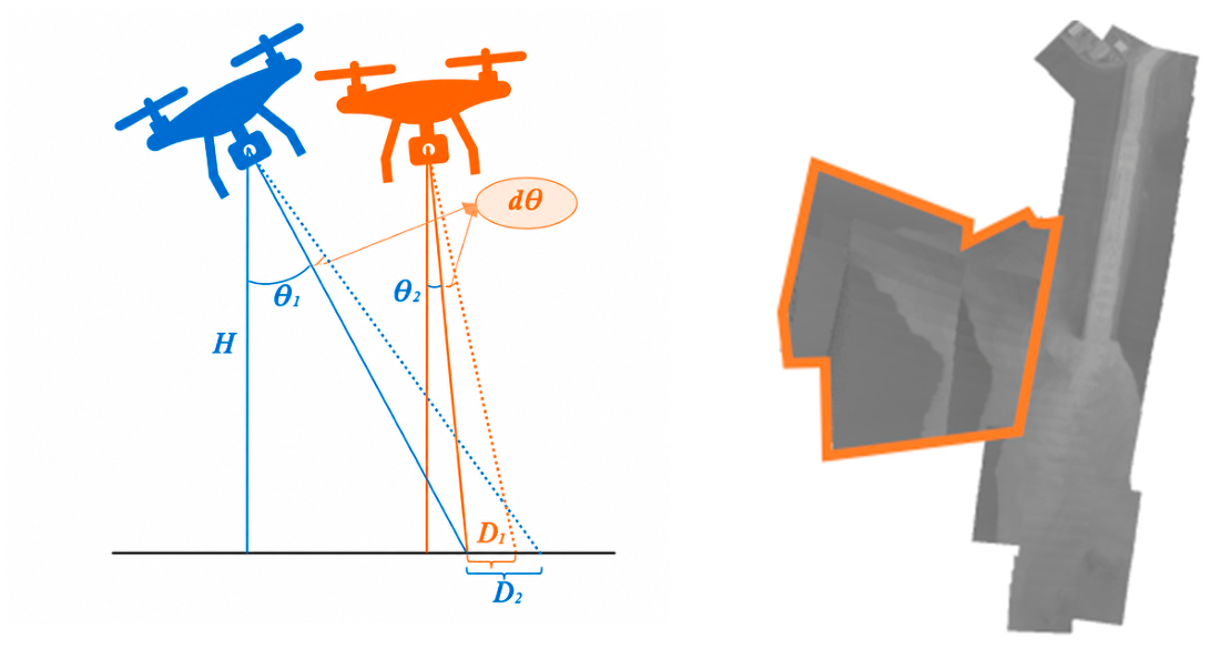
This strategy first utilizes the high-precision position and orientation system (POS) data provided by the real-time kinematic (RTK) system onboard the UAV to perform direct georeferencing and orthorectification on each image, thereby bypassing the reliance on image texture. Nevertheless, we found that a key source of error still exists: during the execution of a “bow-tie” flight mission, the UAV’s attitude, especially its yaw angle, undergoes drastic and non-linear changes during the turning phases of the flight path. This change causes the camera lens to tilt, introducing significant geometric distortion into the images, as shown in Figure 4. If these distorted images are directly used in the mosaicking process, they will severely compromise the geometric consistency of the final product.

To address this problem at its source, we propose an automatic method for filtering distorted images based on yaw angle clustering. The logical basis for this method is that in a standard “bow-tie” flight profile, the vast majority of images are captured along two parallel main flight lines, and their yaw angles should theoretically be stably clustered in two roughly opposite directions (e.g., 0° and 180°). Based on this a priori knowledge, we perform K-Means clustering analysis (K = 2) on the yaw angle data of all images collected in each sub-region. This algorithm can automatically identify the two cluster centers representing the two main flight headings. Images whose yaw angle values significantly deviate from these two centers can be identified with high accuracy and automation as distorted images captured during the non-steady-state turning process.

Before the mosaicking process begins, these identified distorted images are discarded. This step effectively filters the input data source, ensuring that all images participating in the mosaicking have similar and stable attitudes, thereby significantly improving the geometric quality and internal consistency of the final orthoimage.

The orthoimage obtained after geometric processing has pixel values that record the uncalibrated thermal radiance received by the sensor. The next step is to convert these radiance values into physically meaningful temperature values. This study utilizes a single-channel temperature retrieval algorithm integrated into the official DJI software development kit (SDK) (DJI SDK version [3.13]) to perform pixel-wise calculations on the orthoimage.

Since the UAV’s infrared sensor has only one thermal infrared channel, the single-channel algorithm is more suitable for retrieving sea surface temperature. The algorithm divides the radiation received by the thermal infrared sensor into three parts: the thermal radiation from the earth’s surface received by the sensor, the upwelling atmospheric radiation, and the downwelling atmospheric radiation, as shown in the following equation:

$$L_i=\tau \epsilon B\left(T_s\right)+L_{ai}^{\uparrow }+\tau \left(1-\epsilon \right)L_{ai}^{\downarrow }$$

(1)

where $L_{ai}^{\uparrow }$ is the upwelling atmospheric radiation; $L_{ai}^{\downarrow }$ is the downwelling atmospheric radiation; $T_s$ is the sea surface temperature; $B\left(T_s\right)$ is the blackbody thermal radiance intensity of the sea surface within the sensor’s thermal infrared band; $\tau$ is the atmospheric transmittance; and $\epsilon$ is the water surface emissivity.

After processing with this algorithm, we obtained an initial temperature distribution map covering the entire study area. It is important to emphasize that the temperature obtained at this stage is the sea surface brightness temperature. It can accurately reflect the relative spatial distribution pattern of the sea surface temperature, but due to the inherent uncertainty in estimating atmospheric parameters and the sensor’s own systematic errors, a complex non-linear bias still exists between its values and the true absolute sea surface temperature. Therefore, we define this temperature product as the “UAV-retrieved relative temperature,” and it will serve as the core input feature for the subsequent machine learning model.

3.2. Spatiotemporal Matching of UAV and In-Situ Data

To train and evaluate the subsequent machine learning correction model, it is necessary to construct a high-quality dataset that requires precise spatiotemporal matching between the discrete in-situ transect temperature measurements and the continuous UAV temperature imagery. This data preparation step is a key prerequisite for ensuring that the model can learn true physical laws. The core of the matching process lies in effectively associating two types of data with different spatiotemporal attributes: the instantaneous areal data acquired by the UAV and the time-series point data from the transect measurements.

To this end, we designed and implemented a set of rigorous matching criteria. In the temporal dimension, considering that sea surface temperature is rapidly influenced by various environmental factors such as solar radiation, wind fields, and tides, we set a 10-min time window to ensure a high degree of synchronicity between the two data types. Specifically, for each in-situ CTD data point with a precise timestamp, we checked whether its recording time $t_{CTD}$ fell within the interval of 10 min before and after the central moment $t_{UAV}$ of the UAV image acquisition period for the corresponding sub-region. The temporal matching condition is formally expressed as:

$$\left|t_{CTD}-t_{UAV}\right|\le {∆t}_{threshold}$$

(2)

where ${∆t}_{threshold}$ is set to 10 min. Only the in-situ points that met this condition were considered temporally valid and proceeded to the next step of spatial matching. The establishment of this standard represents a judicious trade-off between ensuring data synchronicity and retaining a sufficient number of samples. In the spatial dimension, for all CTD data points that passed the temporal screening, we used their synchronously recorded high-precision DGPS coordinates for precise georeferencing on the UAV orthoimage. The spatial matching window was strictly set to a single pixel; that is, we only extracted the “UAV-retrieved relative temperature” value of the unique pixel into which the DGPS coordinate point fell, to serve as the remote sensing observation corresponding to the in-situ measured CTD temperature value. Although this “point-to-point” matching method is strict, it can most directly reflect the sensor’s performance at a specific location, avoiding the smoothing out of local details that can result from spatial averaging.

After the above rigorous spatiotemporal matching process, all CTD data that did not meet the conditions and points that could not be matched to a corresponding pixel were discarded. Ultimately, we successfully integrated the two data sources, constructing a high-quality dataset containing 171,823 valid matched pairs. Each record in this dataset includes a complete set of information, such as the UAV-retrieved relative temperature, the in-situ absolute temperature (as the ground truth for the output), longitude, latitude, tidal type, and tidal state, providing a solid data foundation for the subsequent development of a complex machine learning model capable of perceiving spatial and environmental changes.

3.3. High-Accuracy Temperature Correction Based on Machine Learning

Our preliminary exploratory data analysis indicates that there is a complex non-linear relationship between the UAV-retrieved relative temperature and the in-situ absolute temperature, a relationship that is jointly modulated by spatial location and the marine dynamic environment. Traditional linear regression algorithms, due to their inherent linear assumption, are unable to effectively capture this complex pattern, resulting in limited correction accuracy that cannot meet the needs of fine-scale monitoring of thermal discharge from nuclear power plants. Therefore, to achieve high-accuracy temperature correction, we chose to develop a MLP model, which has a stronger non-linear fitting capability. As a classic feed-forward neural network, the MLP has been proven to be a powerful universal function approximator, theoretically capable of fitting any complex continuous function, making it an ideal tool for solving such data-driven non-linear regression problems.

The core innovation of our method lies in designing a multi-dimensional input feature system for the MLP model that can perceive spatial location and marine environmental status, in order to cope with the complexity of the nuclear power plant’s thermal discharge under different spatiotemporal contexts. The specific input features include four levels: first, the core observational feature, which is the relative temperature value directly retrieved by the UAV and serves as the basis for the model’s correction; second, the spatial geographic features, which are the longitude and latitude coordinates of each sample point, a feature designed to enable the model to learn about geographically related systematic biases, such as differences between near-shore and offshore areas or areas with different water depths; third, the marine environmental features, which are the tidal type (spring, intermediate, neap) and tidal state (maximum flood, flood slack, maximum ebb, ebb slack) during the observation period, a feature designed to help the model understand how changes in water mixing and stratification under different marine dynamic conditions affect the relationship between remote sensing temperature and true temperature; and fourth, the seasonal background feature (summer and winter) to help the model learn the baseline thermal differences across different climatic contexts. The input feature vector can thus be defined as:

$$x=\left[T_{UAV},Longitude,Latitude,{{Season}_{encoded},TidalType}_{encoded},{TidalState}_{encoded}\right]$$

(3)

where $Season,TidalType$ and $TidalState$ are one-hot encoded categorical variables. The model’s output is set to the in-situ measured sea surface absolute temperature.

Before feeding the data into the model, we performed necessary preprocessing steps. For continuous numerical features such as temperature, longitude, and latitude, we used standardization to scale them to a distribution with a mean of 0 and a variance of 1. This not only accelerates model convergence but also prevents features of different scales from having an imbalanced influence on the training process. For discrete categorical features such as tidal type and tidal state, we used one-hot encoding to convert them into a binary vector format that the model can effectively understand, thereby avoiding the introduction of erroneous ordinal relationships. While continuous hydrodynamic variables (e.g., precise flow velocity or tidal elevation) contain richer physical information, acquiring high-resolution, synchronous 2D continuous flow fields across the entire massive study area during rapid UAV flights is operationally unfeasible without complex coupled numerical models. Therefore, categorical tidal states act as practical, highly accessible macroscopic proxies. For instance, slack tides represent periods of weak turbulence and localized heat accumulation, while maximum flows represent rapid advection. These categorical proxies proved sufficient to capture the main hydrodynamic context and significantly improve correction accuracy. It is also worth noting that basic meteorological factors (e.g., atmospheric humidity, air temperature) were implicitly accounted for during the initial radiative transfer retrieval step using the DJI SDK. While incorporating real-time, high-resolution 2D meteorological data (such as localized wind speed or solar irradiance) could theoretically further refine the model, acquiring such data synchronously across the entire study area during flight missions is operationally unfeasible. Furthermore, within the strict 1-h flight window for each tidal state, these meteorological factors remained relatively stable, and their transient impact was significantly smaller than the drastic advection driven by tidal currents. Thus, utilizing macroscopic environmental proxies (Season and Tidal State) effectively captures the dominant non-linear biases without introducing noise from low-resolution weather variables.

Given the exceptionally high accuracy expectations, rigorous measures were implemented throughout the training phase to mitigate potential overfitting and ensure the model’s true generalization capability. First, the constructed matched dataset (171,823 pairs) was randomly partitioned into a training set and a test set at an 8:2 ratio. The test set was kept strictly independent and was never exposed to the model during training or hyperparameter tuning. Second, we systematically optimized the model’s key hyperparameters using a combination of grid search and 5-fold cross-validation on the training set, which avoids biases from any specific validation split. Specifically, considering the dataset size and feature dimensionality, overly wide or deep network structures are highly prone to overfitting. We tested various hidden layer configurations, regularization strengths, and learning rates (

Table 1. Grid search space and final selected hyperparameters for the MLP model.

Hyperparameter	Search Space	Final Selected Value
Hidden layer sizes	(30,), (50,), (50, 25), (100, 50), (200, 100)	(100, 50)
alpha	0.1, 0.01, 0.001	0.01
Learning rate init	0.001, 0.01	0.01
Max iter	1000, 2000	1000

). The results indicated that the two-layer funnel structure (100, 50) provided the optimal balance between high prediction accuracy and computational efficiency, effectively constraining the model capacity.

The finally determined MLP model employs a network structure that includes an input layer, two hidden layers (with 100 and 50 neurons, respectively), and an output layer. In the hidden layers, we chose the rectified linear unit (ReLU) as the activation function to enhance the model’s non-linear expressive power and effectively mitigate the vanishing gradient problem. The training process was driven by the Adam optimizer, a computationally efficient and practically effective gradient descent algorithm, with the learning rate set to 0.01. To further explicitly prevent model overfitting and improve its performance on unseen data, we introduced L2 regularization (penalty parameter set to 0.01) to penalize large weights, and enabled an early stopping mechanism to automatically terminate training when validation performance ceased to improve, preventing the network from memorizing noise.

To comprehensively and objectively evaluate the model’s performance, we used three widely used regression evaluation metrics: the root mean square error (RMSE), which reflects the dispersion of prediction errors and is more sensitive to larger errors; the mean absolute error (MAE), which intuitively represents the average difference between predicted and true values and has the same units as the target variable (°C); and the coefficient of determination (R²), which indicates the extent to which the model explains the variance in the data, with values closer to 1 indicating a better model fit. To rigorously demonstrate the superiority of our proposed MLP model, we also conducted a strict accuracy comparison of its performance against two traditional baseline models, standard linear regression and fifth-order polynomial regression, on the exact same test set.

4. Experiments and Results

This chapter presents and analyzes the evaluation results of the temperature correction models. First, by evaluating the performance of the baseline models, the limitations of traditional methods are revealed to justify the necessity of introducing a non-linear model. Subsequently, the overall accuracy, reliability, and robustness of the proposed MLP model will be detailed. Finally, through a quantitative comparison with the baseline models, the superiority of the MLP model is comprehensively validated, and its final application effect in the spatiotemporal pattern retrieval of the thermal discharge is demonstrated.

4.1. Seasonal Variability and Limitations of Baseline Models

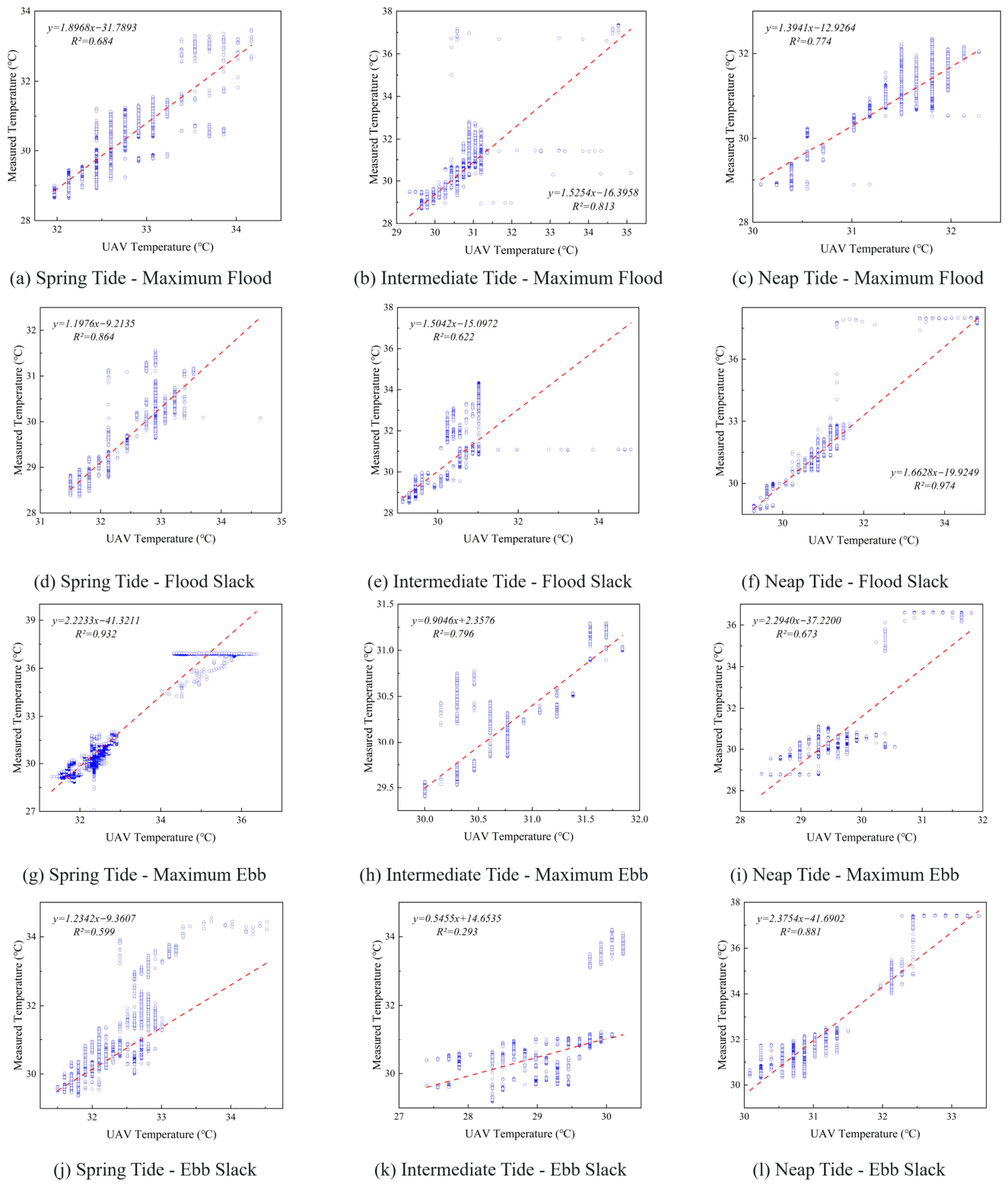
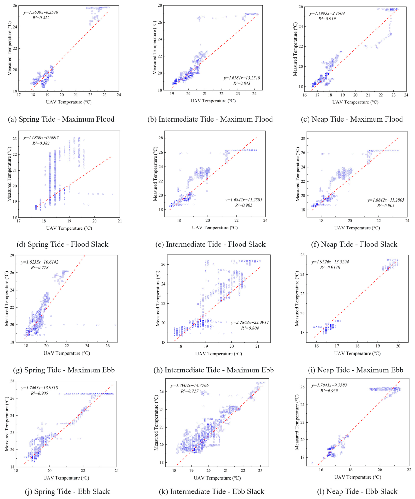
To establish a methodological comparative baseline, this study first evaluated the applicability of the standard linear regression model for the temperature correction task. We constructed independent linear models for both Summer and Winter datasets under 12 different tidal conditions, aiming to quantify the degree of linear correlation between the UAV-retrieved relative temperature and the in-situ absolute temperature, and to diagnose any potential seasonal variability in this relationship.

The evaluation results, as depicted in the scatter plots for Summer (Figure 5) and Winter (Figure 6), reveal that the linear relationship between the two temperature variables exhibits a high degree of condition-dependency, instability, and significant seasonal variation.

In the Summer dataset (Figure 5), the model’s performance shows extreme sensitivity to the tidal state. While under certain quiescent conditions, such as the neap tide flood slack (R² = 0.974), the model demonstrated strong explanatory power, its performance significantly deteriorated in most other scenarios, especially under hydrodynamically complex tidal phases. The inherent limitations of the linear method were fully exposed under conditions such as the intermediate tide maximum flood (R² = 0.684) and the neap tide ebb slack (R² = 0.293), where low R² values and highly discrete data distributions confirmed the model’s failure.

Interestingly, the Winter dataset (Figure 6) presents a different pattern. Although still variable, the linear correlation in Winter was generally more stable and stronger than in Summer across most tidal conditions. This suggests that the relationship between UAV-retrieved and in-situ temperatures is less perturbed by hydrodynamic changes during the winter. This seasonal discrepancy strongly indicates that a single, static linear transformation is far from sufficient to describe a complex functional relationship that is fundamentally modulated not only by short-term environmental factors (tidal phase) but also by long-term seasonal shifts. In other words, the systematic bias is a variable that evolves dynamically with both the immediate hydrodynamic environment and the broader seasonal context.

In summary, the evaluation of the baseline models confirmed from both visual and quantitative perspectives that there exists a significant non-linear, time-variant, and seasonally-dependent association between the two temperature datasets. This finding not only exposes the fundamental deficiencies of traditional linear correction methods but also provides a compelling rationale for the introduction of a more advanced non-linear model. It highlights the necessity of developing an algorithm, such as the MLP model proposed in subsequent sections, that can simultaneously learn and adapt to both short-term dynamic conditions and long-term seasonal patterns.

4.2. MLP Model Performance Evaluation

4.2.1. Overall Accuracy and Generalization Capability

To rigorously evaluate the generalization ability of the developed MLP model on unseen data, we applied it to an independent test set comprising data from both summer and winter seasons, and conducted a quantitative analysis from multiple dimensions.

The evaluation results show that the model exhibits exceptional prediction accuracy and high reliability across different climatic contexts. Across the entire combined test set, the model’s RMSE was 0.2561 °C, the MAE was 0.1523 °C, the mean relative error (MRE) was 0.0062, and the coefficient of determination (R²) was as high as 0.9980. The extremely low error metrics, combined with an R² value close to 1, jointly demonstrate that the model can retrieve the true absolute sea surface temperature with high precision from the input UAV-retrieved relative temperature and auxiliary spatiotemporal features. 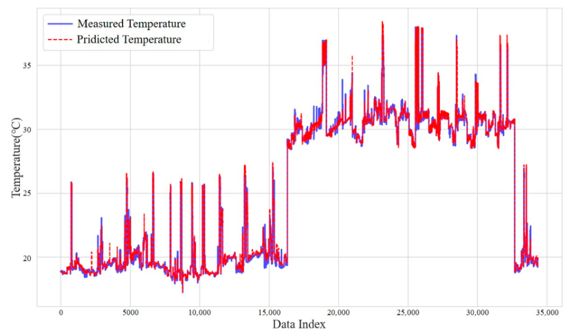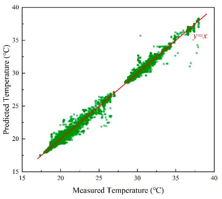Figure 7 shows a comparison between the test values and the predicted values. Their distributions are remarkably close and tend tightly towards the ideal fit line.

The scatter plot comparing predicted and measured values in Figure 8 provides intuitive visual evidence of the model’s overall performance. All data points are tightly and uniformly distributed on both sides of the 1:1 ideal fit line (y = x), with no obvious systematic deviation or heteroscedasticity observed. This indicates a high degree of consistency between the model’s predicted values and the true values across the entire temperature range spanning two seasons.

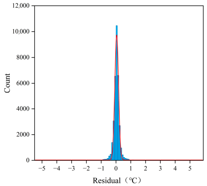
To further investigate the distribution characteristics of the errors, Figure 9 presents a histogram of the model’s prediction residuals (i.e., predicted value minus measured value). The residual distribution exhibits approximately normal characteristics, with its central peak tightly centered around 0, indicating that the model’s predictions are unbiased. Quantitative statistical analysis of the error intervals shows that 89.6% of the samples have an absolute prediction error of less than 0.3 °C, while 96.0% of the samples have an absolute error of less than 0.5 °C. This highly concentrated error distribution corroborates, from a statistical perspective, the high accuracy and reliability of the MLP model.

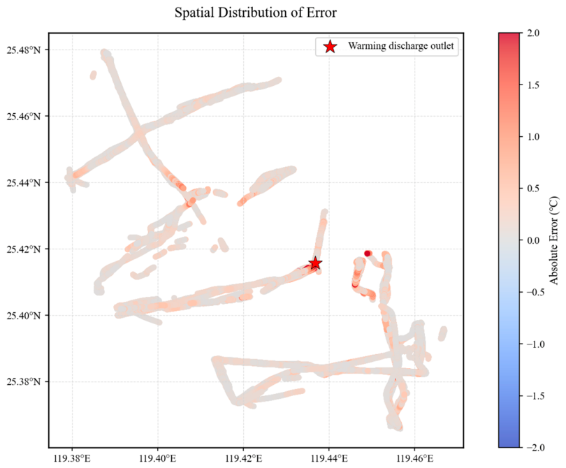
While global metrics provide an overall assessment, understanding the spatial distribution of errors is crucial. Figure 10 presents the spatial error map (residuals between predicted and in-situ measurements) for a representative tidal condition. The errors are generally uniformly distributed and low across the open water. However, slightly higher residual errors are occasionally concentrated in the immediate vicinity of the thermal discharge outlet, where the spatial thermal gradients are extremely steep and hydrodynamics are highly turbulent. This spatial pattern aligns with physical expectations.

4.2.2. Seasonal Adaptability and Robustness Under Varying Tidal Conditions

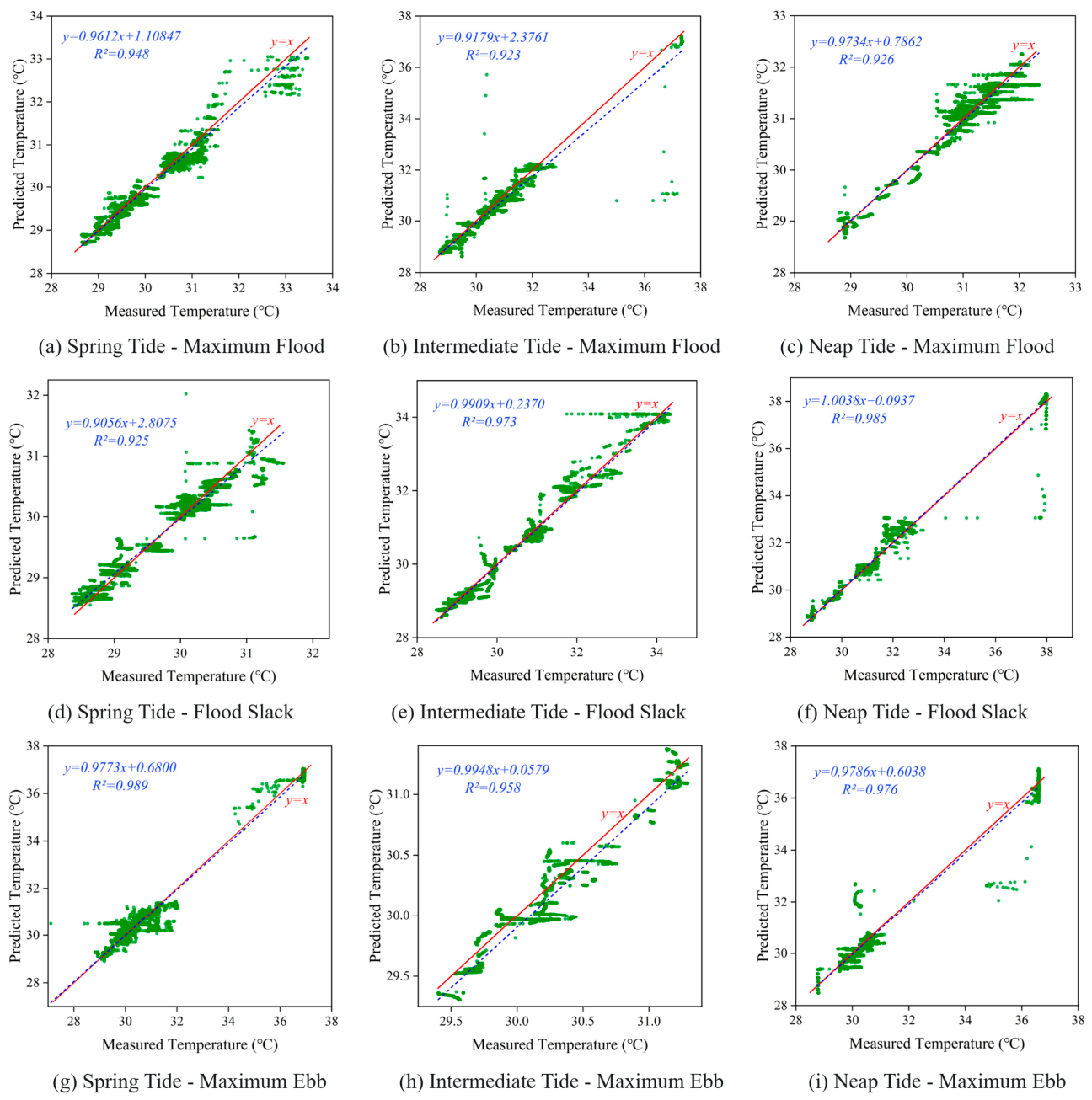
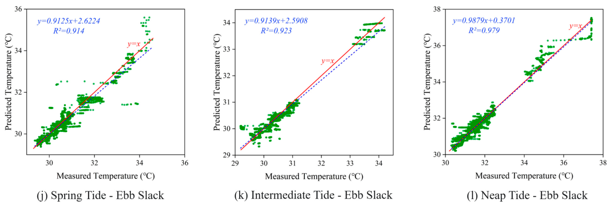
In addition to evaluating the overall performance, it is crucial to verify the model’s adaptability and stability under different marine dynamic environments and climatic backgrounds, i.e., its spatiotemporal robustness. To this end, we stratified the test set by season (Summer vs. Winter) and the 12 different tidal conditions, and independently evaluated the correction effect of the MLP model on each subset.

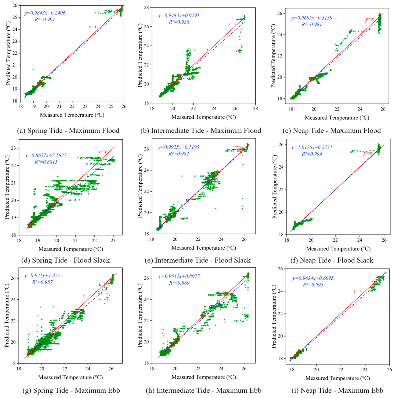
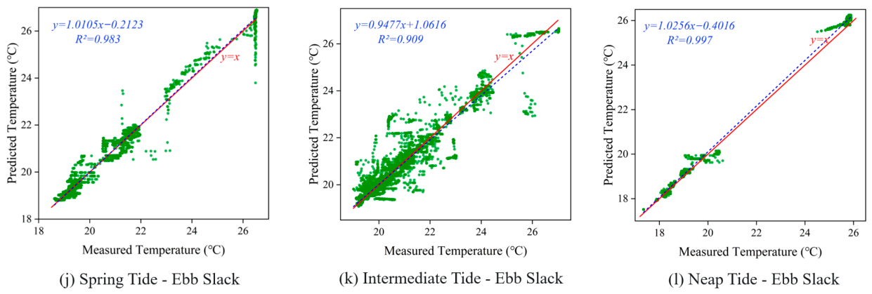
As shown in the series of scatter plots (Figure 11 for Summer and Figure 12 for Winter), under almost all combinations of tidal types and states, the temperature values corrected by the MLP model and the in-situ measured values exhibit a very strong linear correlation. In the vast majority of conditions across both seasons, the coefficient of determination R² is consistently above 0.9, standing in stark contrast to the drastic fluctuations and poor performance of the linear regression model discussed in Section 4.1.

Notably, a detailed comparison reveals a distinct seasonal pattern in the correction performance. Overall, the corrected R² values in Winter are generally higher than those in Summer (with minor exceptions such as the spring tide flood slack and intermediate tide ebb slack). Correspondingly, the MAE in Winter is generally lower than in Summer across most tidal states. This indicates that while the MLP model performs excellently in both seasons, its correction effect in Winter is even closer to the measured truth.

This seasonal discrepancy can be attributed to the differing physical characteristics of the water body: summer thermal plumes exhibit higher temperature extremes and sharper spatial gradients due to stronger solar radiation and thermal stratification, which increases the inherent difficulty of remote sensing correction. In contrast, winter temperatures are distributed more uniformly due to better vertical mixing, providing a relatively more stable signal for the model.

To explicitly justify the necessity of training on a combined dataset and incorporating ‘Season’ as an input feature, we conducted a cross-season transfer experiment. When the model was trained exclusively on Summer data and tested on Winter data, the prediction accuracy degraded drastically (RMSE = 7.709 °C, MAE = 7.307 °C, R² = −23.138). The inverse experiment (trained on Winter, tested on Summer) yielded similarly poor results (RMSE = 5.118 °C, R² = −9.744). This confirms that there is a severe domain shift between summer and winter due to fundamental differences in background water temperatures and atmospheric conditions. Therefore, directly generalizing a single-season model is unfeasible without domain adaptation; explicitly incorporating the seasonal contextual feature is mandatory for robust cross-seasonal correction.

This finding is of great significance: it indicates that by incorporating environmental factors such as “Season” and “Tidal State” as explicit input features, the MLP model has successfully learned and internalized the complex modulations of different marine dynamic conditions on the thermal remote sensing signal. The model adaptively adjusts its internal non-linear mapping according to the specific spatiotemporal “context,” thereby precisely compensating for systematic biases under varying seasonal and tidal conditions. Therefore, these consistently high-accuracy results strongly demonstrate that our proposed model possesses excellent robustness for continuous monitoring in dynamic coastal environments.

4.3. Comparative Accuracy Analysis of Multiple Models

To comprehensively and objectively highlight the superiority of the MLP model proposed in this study for the UAV temperature correction task, this section conducts a systematic accuracy comparison between this model and two widely used traditional regression methods: standard linear regression, fifth-order polynomial regression, Support Vector Regression (SVR), and Random Forest (RF). Crucially, to verify the model’s spatiotemporal robustness, this comparison is expanded across both Summer and Winter datasets. All models were trained on the same training set and evaluated on the exact same test set.

Table 2. Summer comparative accuracy assessment of different models under 12 tidal conditions.

		Spring Tide				Intermediate Tide				Neap Tide
Model		Flood Slack	Maximum Flood	Maximum Ebb	Ebb Slack	Flood Slack	Maximum Flood	Maximum Ebb	Ebb Slack	Flood Slack	Maximum Flood	Maximum Ebb	Ebb Slack
Linear Regression	RMSE	0.260	0.448	0.642	0.450	0.811	0.507	0.246	0.571	0.393	0.362	1.069	0.500
	MAE	0.158	0.341	0.474	0.288	0.473	0.285	0.172	0.388	0.252	0.289	0.876	0.394
	R2	0.864	0.684	0.932	0.599	0.622	0.813	0.796	0.293	0.974	0.774	0.673	0.881
Polynomial Regression	RMSE	0.251	0.434	0.336	0.407	0.726	0.480	0.219	0.463	0.344	0.322	0.504	0.355
	MAE	0.157	0.328	0.230	0.258	0.479	0.278	0.149	0.346	0.215	0.243	0.299	0.269
	R2	0.873	0.703	0.981	0.672	0.697	0.833	0.838	0.536	0.980	0.821	0.927	0.940
SVR	RMSE	0.224	0.315	0.462	0.246	0.277	0.433	0.131	0.298	0.306	0.239	0.510	0.271
	MAE	0.131	0.194	0.262	0.143	0.176	0.203	0.106	0.155	0.148	0.170	0.228	0.170
	R2	0.899	0.844	0.965	0.880	0.956	0.864	0.942	0.807	0.984	0.902	0.926	0.965
MLP	RMSE	0.194	0.191	0.262	0.212	0.220	0.353	0.151	0.190	0.302	0.214	0.295	0.212
	MAE	0.144	0.148	0.155	0.135	0.163	0.192	0.129	0.135	0.178	0.167	0.145	0.157
	R2	0.925	0.943	0.989	0.911	0.972	0.910	0.923	0.922	0.985	0.921	0.975	0.979

and

Table 3. Winter comparative accuracy assessment of different models under 12 tidal conditions.

		Spring Tide				Intermediate Tide				Neap Tide
Model		Flood Slack	Maximum Flood	Maximum Ebb	Ebb Slack	Flood Slack	Maximum Flood	Maximum Ebb	Ebb Slack	Flood Slack	Maximum Flood	Maximum Ebb	Ebb Slack
Linear Regression	RMSE	0.571	0.517	0.650	0.488	0.522	0.466	0.795	0.673	0.272	0.452	0.514	0.640
	MAE	0.321	0.447	0.448	0.388	0.356	0.313	0.639	0.502	0.191	0.308	0.432	0.459
	R2	0.382	0.822	0.778	0.905	0.905	0.843	0.804	0.727	0.988	0.919	0.918	0.939
Polynomial Regression	RMSE	0.542	0.245	0.458	0.382	0.349	0.371	0.532	0.563	0.176	0.420	0.240	0.431
	MAE	0.298	0.190	0.296	0.248	0.182	0.185	0.257	0.372	0.104	0.269	0.191	0.371
	R2	0.444	0.960	0.890	0.942	0.958	0.900	0.912	0.809	0.955	0.930	0.982	0.972
SVR	RMSE	0.263	0.151	0.325	0.271	0.297	0.385	0.429	0.427	0.183	0.284	0.164	0.431
	MAE	0.134	0.086	0.202	0.136	0.145	0.163	0.203	0.223	0.112	0.142	0.118	0.199
	R2	0.869	0.985	0.944	0.971	0.969	0.893	0.943	0.890	0.995	0.968	0.992	0.972
MLP	RMSE	0.251	0.128	0.314	0.208	0.227	0.308	0.329	0.393	0.195	0.231	0.167	0.195
	MAE	0.138	0.093	0.203	0.128	0.114	0.180	0.164	0.207	0.118	0.144	0.131	0.153
	R2	0.880	0.989	0.948	0.983	0.982	0.931	0.966	0.907	0.994	0.979	0.991	0.992

provide a detailed list of the three key performance metrics (RMSE, MAE, and R²) for these three models under all 12 tidal conditions in Summer and Winter, respectively.

A vertical comparison of the data in the tables clearly reveals the all-around performance advantage of the MLP model. In all 24 conditions (12 in Summer and 12 in Winter), the MLP model consistently performed the best across all three evaluation metrics, possessing the lowest RMSE and MAE, as well as the highest R². Taking the MAE metric as an example, the MAE values of the MLP model in Summer were stable within a very narrow range of 0.129 °C to 0.192 °C, and even lower in Winter (0.093 °C to 0.207 °C). In stark contrast, the MAE values for linear regression fluctuated sharply between 0.158 °C and 0.876 °C in Summer, and between 0.191 °C and 0.639 °C in Winter. This fully demonstrates that the MLP model is not only more accurate, but its prediction performance is also remarkably reliable and consistent, effectively avoiding the risk of overfitting often seen in polynomial regression under complex conditions.

A deeper quantitative analysis reveals interesting seasonal differences in the magnitude of accuracy improvement brought by the MLP model. Compared to the baseline linear regression, the MLP model in Summer reduced the RMSE by an average of 0.289 °C, reduced the MAE by an average of 0.212 °C, and increased the R² by an average of 0.204. In Winter, the improvement was even more pronounced in terms of absolute error reduction: the MLP model reduced the RMSE by an average of 0.301 °C and the MAE by an average of 0.253 °C (with an average R² increase of 0.134). These metrics indicate that while the MLP model significantly enhances accuracy in both seasons, it yields a greater reduction in absolute errors during the Winter. This suggests that for the Winter data—which inherently exhibited a relatively more stable linear baseline—the MLP’s powerful non-linear mapping capabilities were able to extract even more subtle features and eliminate residual noise, bringing the final corrected values much closer to the true in-situ measurements.

The powerful capability of the MLP model was most vividly demonstrated in “extreme” conditions where traditional methods severely underperformed. For instance, in the summer neap tide ebb slack condition, the linear regression model was almost completely ineffective with an R² of only 0.293, indicating it could explain almost none of the effective variation. However, on the exact same data, the MLP model’s R² remained as high as 0.922, representing an extraordinary improvement in explanatory power of over 214%. Furthermore, even for conditions where traditional methods achieved a relatively good fit, the MLP model showed significant accuracy improvements on top of the existing results. Taking the summer neap tide flood slack as an example, polynomial regression had already achieved a very good performance (R² = 0.980). The MLP model went a step further, increasing the R² to 0.985 while simultaneously reducing the RMSE from 0.344 °C to 0.302 °C.

Furthermore, we compared the MLP with advanced machine learning models including SVR and RF. While RF achieved excellent numerical accuracy on the test set (RMSE = 0.193, MAE = 0.121, R² = 0.998 in Summer), applying the trained RF model to generate spatial SST maps resulted in obvious blocky artifacts, lacking physical continuity (Figure 13). SVR showed lower stability under certain tidal conditions. The MLP, utilizing continuous activation functions, generates much smoother and physically more realistic thermal gradient transitions over the sea surface, making it the optimal choice overall.

In summary, this series of detailed quantitative comparisons across two seasons fully illustrates, from multiple dimensions, the powerful capability and absolute advantages of the machine learning model that fuses multi-dimensional spatiotemporal features in solving complex non-linear remote sensing correction problems.

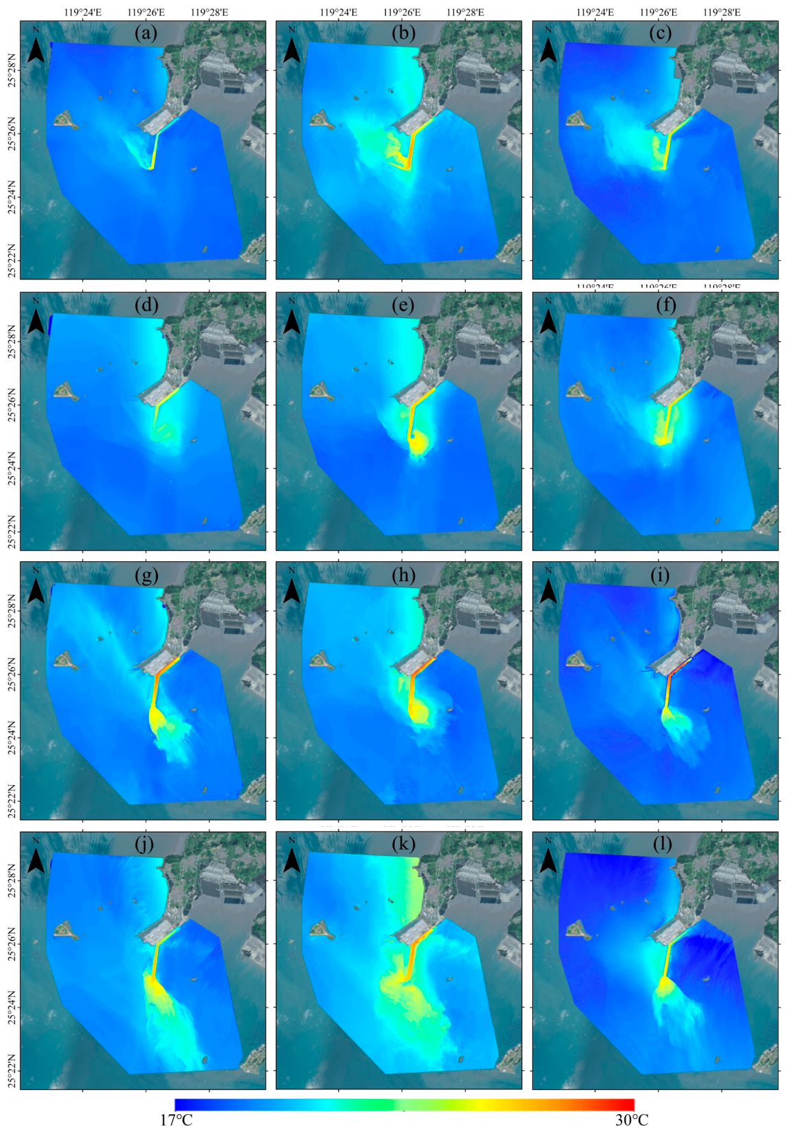
4.4. Retrieval of the Spatiotemporal Distribution Pattern of the Nuclear Power Plant’s Thermal Discharge

After having fully validated the exceptional performance, robustness, and seasonal adaptability of the MLP model in the preceding sections, we applied this trained model as the final correction tool to the entire study area’s UAV orthoimages.

This process was carried out on a pixel-by-pixel basis: for each pixel in the image, we extracted its UAV-retrieved relative temperature and longitude/latitude coordinates, and combined them with the corresponding seasonal and tidal condition information. These were used jointly as inputs for the model to predict the absolute sea surface temperature (SST) for that specific pixel. Through this automated process, we successfully generated high-spatial-resolution (0.67 m), high-accuracy SST distribution maps covering all 24 typical conditions across both summer and winter seasons. These SST maps are not only accurately calibrated numerically, but they also spatially preserve the rich details provided by UAV remote sensing, offering unprecedented high-quality data for in-depth analysis of the spatiotemporal evolution patterns of the nuclear power plant’s thermal plume under varying climatic and hydrodynamic contexts.

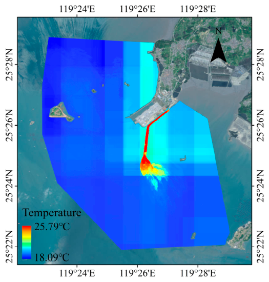
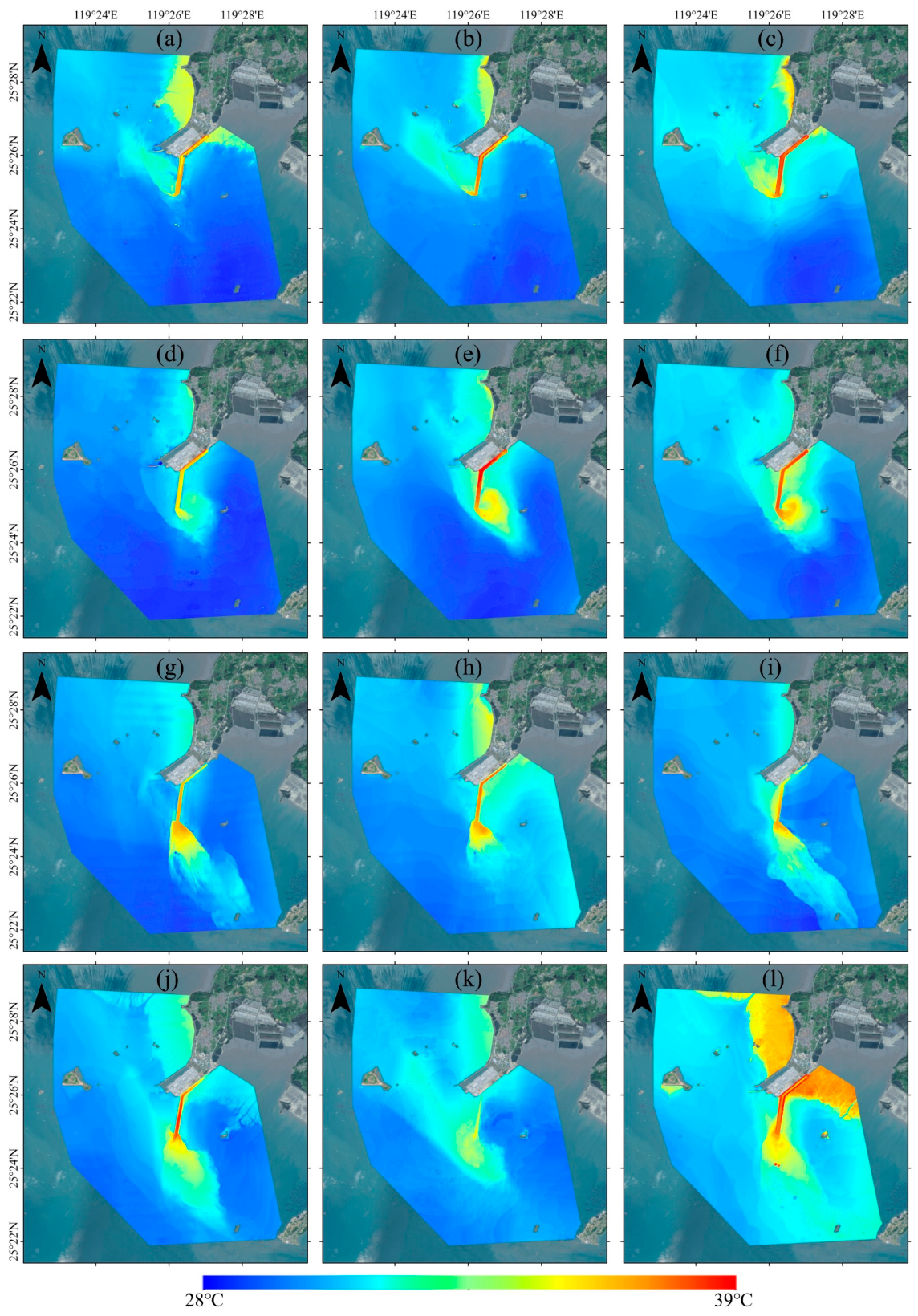
A comparative analysis of the retrieved SST maps across the two seasons reveals distinct seasonal thermal characteristics. In Summer (Figure 14), the thermal plume exhibits significantly higher temperature extremes and sharper spatial thermal gradients. This is primarily due to stronger solar radiation and higher background water temperatures, which intensify the thermal stratification of the surface water and hinder vertical mixing, making the plume’s diffusion boundary more complex and challenging to correct. In contrast, during Winter (Figure 15), the background sea temperature is lower and distributed more uniformly. Driven by stronger wind-induced vertical mixing and heat dissipation, the thermal plume’s contour appears clearer and visually more stable, with a smoother transition zone. This visual evidence perfectly aligns with the quantitative findings in Section 4.3, visually explaining why the model achieved even lower absolute errors (MAE/RMSE) on the Winter dataset.

Despite these seasonal baseline differences, the series of high-accuracy SST maps intuitively and clearly reveals how the morphology, extent, and diffusion path of the Fuqing nuclear power plant’s thermal plume are finely and consistently regulated by tidal dynamics. The strength of the tidal current plays a dominant controlling role in the morphology of the plume. At moments of peak tidal velocity, during maximum flood or maximum ebb, the strong hydrodynamic transport causes the thermal plume to be significantly elongated, forming a narrow, distinct, strip-like structure that diffuses over long distances along the direction of the current. In sharp contrast, at moments when the tidal velocity is close to zero (flood slack or ebb slack), the thermal discharge loses the strong transport of external forces and mainly relies on its own thermal buoyancy and inertia to accumulate near the discharge outlet. Consequently, its morphology appears as a relatively concentrated, regularly outlined globular or tongue-like structure, often with a core area of extremely high temperature.

Furthermore, the direction of the tidal current strictly dictates the transport path of the thermal discharge. By comparing the flood and ebb tides, the “pendulum-like” transport effect of the thermal plume can be clearly observed regardless of the season. During the flood tide period, the overall diffusion direction of the thermal plume is significantly biased towards the interior of the bay. Conversely, during the ebb tide period, the thermal plume undergoes a nearly 180-degree turn, diffusing towards the exterior of the bay (i.e., the open sea).

In conclusion, these high-resolution, high-accuracy, cross-seasonal SST retrieval results not only successfully demonstrate the technical superiority and broad applicability of our proposed MLP-based method, but more importantly, they provide a solid and reliable data foundation for subsequent, more in-depth quantitative analysis. This includes accurately calculating the area of the temperature rise envelope under different seasonal and tidal conditions, and comprehensively assessing the scope and intensity of the nuclear power plant’s thermal impact on the marine ecosystem.

5. Conclusions

Addressing the dual challenges of large-scale, high-timeliness observation and high-accuracy quantitative retrieval in the monitoring of near-shore thermal discharges from nuclear power plants, this study successfully developed and validated an innovative monitoring paradigm that integrates coordinated multi-UAV remote sensing with machine learning. Through comprehensive case studies conducted at the Fuqing Nuclear Power Plant, the feasibility, advancement, and high reliability of this technical workflow were rigorously demonstrated.

The core methodological contribution of this study lies in the development of a Multi-Layer Perceptron (MLP) temperature correction model that fuses multi-dimensional spatiotemporal and environmental features. By innovatively incorporating key contextual factors, namely geographical coordinates, tidal status, and seasonal backgrounds—into the correction process, the model effectively overcomes the limitations of traditional linear methods in handling complex, non-linear thermodynamic relationships. Furthermore, to ensure a high-quality data foundation for modeling, we proposed a robust image filtering strategy based on yaw angle clustering, which successfully resolved the key technical bottleneck of severe geometric distortion during the mosaicking of UAV imagery over vast, textureless water surfaces.

Quantitative results demonstrate that the proposed MLP model exhibits exceptional performance and robustness. On an independent test set comprising data from both summer and winter seasons, the model achieved an R² of 0.9980, an RMSE of 0.2561 °C, and a MAE as low as 0.1523 °C. Through detailed comparisons, the MLP model significantly outperformed traditional baseline regression models across all 24 distinct tidal conditions spanning both seasons. Notably, the model effectively captured the seasonal thermal heterogeneity, achieving even higher absolute accuracy during the Winter due to the relatively uniform vertical mixing of the water column. Ultimately, utilizing this model, we successfully generated a series of high-resolution, cross-seasonal sea surface temperature distribution maps, which intuitively revealed the intricate spatiotemporal evolution and “pendulum-like” diffusion patterns of the thermal plume driven by varying tidal dynamics.

In summary, this study not only provides an innovative, data-driven correction approach for the quantitative application of UAV thermal infrared remote sensing but, more importantly, it establishes a technologically advanced, highly accurate, and rapid-response solution for the fine-scale, periodic regulation of near-shore thermal environments. It should also be noted that nuclear power plant thermal plumes represent a highly specific monitoring scenario. They exhibit unique thermal dynamics characterized by continuous, high-volume discharges and extremely steep temperature gradients, which may differ from natural riverine outflows or other industrial discharges. Furthermore, strict regulatory constraints and no-fly zones near nuclear facilities often limit the flexibility of UAV flight trajectories, which in turn underscores the necessity of our automated mosaicking optimization strategy. Regarding practical deployment, while the proposed methodological framework and feature engineering strategy are highly transferable to other coastal or inland aquatic environments, the specific trained model weights are inherently site-dependent. Direct application to a new location without site-specific retraining would yield suboptimal results due to varying baseline water temperatures and localized hydrodynamics. Nevertheless, high accuracy can be rapidly achieved in new environments by simply fine-tuning the model with a small amount of local in-situ data, demonstrating the low transfer cost of this paradigm. Since the cross-seasonal adaptability of this method has been validated, future work will focus on integrating these high-resolution 2D surface temperature maps with 3D hydrodynamic numerical models to uncover the vertical dispersion mechanisms of thermal plumes, and exploring spatially-aware deep learning architectures (e.g., Convolutional Neural Networks or Graph Neural Networks). While our point-wise MLP is computationally efficient and meets practical accuracy requirements, spatially-aware models could further leverage local spatial autocorrelation to improve boundary sharpness and feature extraction directly from thermal imagery.