Cascaded Local–Nonlocal Pansharpening with Adaptive Channel-Kernel Convolution and Multi-Scale Large-Kernel Attention

Highlights

What are the main findings?

• A cascaded local–nonlocal pansharpening network (CLNNet) was developed to progressively refine spatial details and spectral fidelity by stacking PLNF modules.
• Coupling adaptive channel-kernel convolution with multi-scale large-kernel attention within each PLNF improved texture preservation and spectral fidelity.

What are the implications of the main findings?

• The developed CLNNet could enable the generation of HRMS images for downstream remote sensing applications (e.g., classification and detection).
• The progressive local–nonlocal fusion strategy offers strong potential for other multi-source image fusion tasks requiring both fine textures and long-range dependencies.

Abstract

Pansharpening plays a crucial role in remote sensing applications, as it enables the generation of high-spatial-resolution multispectral images that simultaneously preserve spatial and spectral information. However, most current methods struggle to preserve local textures and exploit spectral correlations across bands while modeling nonlocal information in source images. To address these issues, we propose a cascaded local–nonlocal pansharpening network (CLNNet) that progressively integrates local and nonlocal features through stacked Progressive Local–Nonlocal Fusion (PLNF) modules. This cascaded design allows CLNNet to gradually refine spatial–spectral information. Each PLNF module combines Adaptive Channel-Kernel Convolution (ACKC), which extracts local spatial features using channel-specific convolution kernels, and a Multi-Scale Large-Kernel Attention (MSLKA) module, which leverages multi-scale large-kernel convolutions with varying receptive fields to capture nonlocal information. The attention mechanism in MSLKA enhances spatial–spectral feature representation by integrating information across multiple dimensions. Extensive experiments on the GaoFen-2, QuickBird, and WorldView-3 datasets demonstrate that the proposed method outperforms state-of-the-art methods in quantitative metrics and visual quality.

1. Introduction

With the widespread application of remote sensing technology across various fields and its significant economic benefits, the demand for acquiring high-resolution multispectral (HRMS) images has become increasingly urgent. However, due to the inherent limitations of satellite sensors, direct acquisition of HRMS images is not feasible [1,2]. To address this challenge, pansharpening technology is employed; it fuses low-resolution multispectral (LRMS) images and high-resolution panchromatic (PAN) images to generate HRMS images [3]. HRMS images are widely applied in various domains, including ground-object classification, urban planning, and environmental change monitoring [4,5].

In recent years, image fusion has emerged as a key technology in remote sensing, especially for enhancing pansharpening results. The majority of existing pansharpening techniques can be broadly classified into two categories: traditional methods and deep learning (DL)-based methods. Traditional methods mainly include component substitution (CS) methods, multi-resolution analysis (MRA) methods, and variational optimization (VO) techniques [6,7].

CS-based methods project the multispectral (MS) image into a transform domain to separate spatial and spectral components. The spatial component is then substituted with the PAN image, followed by an inverse transform to obtain the HRMS image. Representative methods include IHS [8], PCA [9], GSA [10], and BDSD [11]. While effective at enhancing spatial details, they often cause spectral distortion. MRA-based methods extract spatial details from the PAN image via multi-resolution decomposition and inject them into the upsampled MS image using spatial filtering [12]. Representative methods include wavelet transform, smoothing filter-based intensity modulation (SFIM) [13], and AWLP [14]. These methods struggle to balance the spatial and spectral qualities [15]. VO-based methods formulate pansharpening as an optimization problem by constructing an energy function to model spatial–spectral correlations [16,17,18]. Though capable of generating high-quality results, they rely heavily on prior knowledge and parameter settings, and often suffer from high computational cost [19].

With the rapid advancement of deep learning in computer vision, its application in pansharpening has attracted increasing attention, offering improved accuracy over traditional methods due to excellent nonlinear modeling and feature extraction capabilities. Huang et al. [20] pioneered this direction by introducing a sparse noise-based autoencoder. Subsequent works widely adopted convolutional neural networks (CNNs) to extract spatial and spectral features for high-quality fusion. Masi et al. [21] demonstrated the effectiveness of a lightweight three-layer CNN, while Deng et al. [22] incorporated conventional detail injection into a CNN-based framework. To improve spatial–spectral fidelity, Wu et al. [23] introduced fidelity constraints via VO + Net, and Wang et al. [24] designed VOGTNet, a two-stage network guided by variational optimization to mitigate noise and preserve structure.

Although CNNs have achieved notable progress in pansharpening, their inherent locality limits their ability to capture long-range dependencies and fuse the features corresponding to LRMS and PAN images. To address these challenges, researchers have introduced multi-scale processing and nonlocal mechanisms into network design. For instance, Yuan et al. [25] proposed a multi-scale and multi-depth CNN with residual learning, while Zhang et al. [26] introduced TDNet, which progressively refines spatial details through a triple–double structure. Jian et al. [27] developed MMFN to fully leverage spatial and spectral features using multi-scale and multi-stream designs. Huang et al. [28] further enhanced fusion quality by incorporating high-frequency enhancement and multi-scale skip connections within a dual-branch framework. Meanwhile, nonlocal operations have been employed to model global dependencies beyond the receptive field of CNNs. Lei et al. [29] proposed NLRNet, a residual network enhanced with nonlocal attention. Wang et al. [30] introduced a cross-nonlocal attention mechanism to jointly capture spatial–spectral features. Inspired by vision transformers, Zhou et al. [31] designed PanFormer, with dual-stream cross-attention for spatial–spectral fusion. In addition, Huang et al. [32] and Yin et al. [33] developed local–global fusion architectures to jointly exploit fine details and contextual information. Khader et al. [34] proposed an efficient network for HRMS and MS image fusion that incorporates dynamic self-attention and global correlation refinement modules. Most local and nonlocal fusion architectures follow a parallel paradigm, where local detail features and global context features are extracted in separate branches and then merged by concatenation, attention, or other fusion operators. While effective, this paradigm may limit deep, iterative interactions between local textures and nonlocal contextual cues.

Despite their effectiveness in capturing global dependencies, these methods still rely on static convolutional operations, limiting their ability to adapt to spatial variations. These have motivated the introduction of adaptive convolution and attention mechanisms to further enhance spatial–spectral feature representation. Lu et al. [35] proposed a spectral–spatial self-attention module to improve detail fidelity and interpretability. Meanwhile, another study [36] designed a self-guided adaptive convolution that generates channel-specific kernels based on content and incorporates global context. Zhao et al. [37] developed a progressive reconstruction network with adaptive frequency adjustment and multi-stage refinement to correct high-frequency distortions. Song et al. [3] further introduced an invertible attention-guided adaptive convolution combined with a dual-domain transformer to jointly model spatial–spectral details and frequency-domain dependencies.

Although DL-based methods have achieved remarkable progress in pansharpening, several critical challenges remain. First, many existing methods struggle to adequately integrate local details and long-range information, leading to incomplete spatial–spectral feature fusion, particularly in scenarios that simultaneously require sharp boundary reconstruction and small-object detail preservation. Second, during nonlocal feature extraction, existing networks lack efficient modules to enhance representational capacity, limiting the balance between fine-detail preservation and global structural consistency and often treating nonlocal dependency modeling independently of local spatial–spectral refinement. Third, conventional convolution operations employ fixed kernels across the entire image, restricting adaptability to spatially varying structures and insufficiently exploiting interband spectral correlations, which hampers adaptive spatial–spectral coupling under heterogeneous land-cover distributions. These limitations lead to degraded fusion quality and further propagate to downstream remote sensing applications, such as land-cover classification and change detection, in the form of boundary ambiguity and band-dependent spectral distortion. Moreover, although multi-scale strategies are widely used, many of them rely on fixed convolutional kernels or generic attention designs, which may be insufficient to jointly address band-dependent spectral distortion and spatial heterogeneity in multi-band remote sensing images.

To address these issues, we propose a cascaded local–nonlocal pansharpening network (CLNNet) that progressively integrates local and nonlocal features through stacked Progressive Local–Nonlocal Fusion (PLNF) modules. Specifically, each PLNF module consists of two main components: an Adaptive Channel-Kernel Convolution (ACKC) block and a Multi-scale Large-Kernel Attention (MSLKA) block. The ACKC block generates channel-specific adaptive kernels to extract fine-grained local spatial details and enhance spectral correlations across bands. Within the MSLKA block, multi-scale large-kernel convolutions (MLKC) with varying receptive fields are employed to capture nonlocal information. In addition, an Attention-Integrated Feature Enhancement (AIFE) module is incorporated to integrate pixel, spectral, and spatial attention mechanisms, thereby performing multi-dimensional enhancement on the input features. The combination of these components enables the network to capture long-range dependencies and enrich feature representations, thereby facilitating consistent fusion of local and nonlocal information. In summary, the main contributions of this paper are as follows:

• We propose a cascaded local–nonlocal pansharpening network that integrates ACKC and MSLKA modules in a sequential manner. This design aims to improve spatial continuity, spectral consistency, and feature complementarity.
• The proposed ACKC module generates channel-specific kernels and introduces a global enhancement mechanism to incorporate contextual information, while preserving spectral fidelity by exploiting spectral correlations across bands.
• We design an MSLKA module that integrates MLKC with AIFE to capture long-range dependencies and enhance multi-dimensional feature fusion. Multiple attention strategies in AIFE further improve nonlocal spatial–spectral information and contextual coherence.

2. Related Work

2.1. Adaptive Convolution

Standard convolution employs fixed kernels across all spatial locations, limiting its adaptability to geometric variations and contextual differences. In contrast, adaptive convolution dynamically generates kernels conditioned on the input content, thereby providing greater flexibility in modeling spatial deformations and varying object scales commonly encountered in visual tasks [38,39]. Early explorations, such as DFN [40], introduced position-specific filters to capture local variations, establishing the foundational link between convolution operations and spatial/channel dimensions. Subsequent methods further improved kernel generation strategies. For example, DYConv [41] aggregates multiple kernel branches through attention-based weighting; Involution [42], on the other hand, reinterprets convolution as a self-attention mechanism operating locally with channel-wise adaptation.

Within the domain of remote sensing image pansharpening, several tailored adaptive convolutional methods have been proposed. LAGConv [43] proposed a generate local-context adaptive convolution kernels, while ADKNet [44] designs a convolution network with source-adaptive discriminative kernels. These methods highlight the importance of specific adaptation strategies in pansharpening tasks. However, despite these advances, most existing adaptive convolution techniques are still limited by their reliance on local and inadequate exploitation of spectral correlations across different bands. This often leads to incomplete spatial–spectral feature fusion and insufficient preservation of fine-grained details. Therefore, adopting strategies that generate channel-specific convolution kernels can provide a balanced solution, facilitating both fine-grained local detail preservation and improved spectral consistency in pansharpening.

2.2. Large-Kernel Attention Mechanism

The attention mechanism can be regarded as a discriminative process that emphasizes informative regions while suppressing irrelevant features [45]. Introduced into computer vision through the Recurrent Attention Model (RAM) [46], attention has been used in numerous visual tasks, including image classification [47,48], object detection [49,50], and semantic segmentation [51,52]. Although attention mechanisms have significantly improved feature representation in various vision tasks, most existing designs rely on global interactions or complex multi-branch architectures, resulting in high computational cost and limited scalability.

To reduce the computational overhead of attention while maintaining long-range modeling capabilities, many recent methods have proposed approximate attention mechanisms. Among them, Large Kernel Attention (LKA) [53] has emerged as a prominent strategy that bridges the gap between convolution and self-attention. By leveraging large-kernel convolutions, LKA captures both local structural features and global context while maintaining adaptability. Unlike self-attention, it avoids the computational overhead of global pairwise comparisons and better accommodates channel-specific characteristics.

In LKA, attention weights are implicitly modeled using large-kernel convolutions rather than explicit dot-product operations. For instance, the RepLK Block approximates the self-attention mechanism using extremely large (e.g., 31 × 31) convolution kernels, demonstrating their effectiveness in modeling both local and nonlocal dependencies. Similarly, Guo et al. [53] proposed the LKA module, which stacks multi-scale depthwise convolutions (e.g., 5 × 5 and 7 × 7) to form a broad receptive field. This structure approximates attention in a linear and efficient manner, showing promising results in image super-resolution tasks.

Instead of using explicit dot-product attention, the LKA module approximates global dependencies through a combination of depthwise and dilated convolutions. As illustrated in Figure 1, a large-kernel convolution is decomposed into a stack of three operations: a depthwise convolution, a dilated depthwise convolution, and a pointwise convolution. This design enables efficient large-receptive-field modeling with minimal computational overhead. These insights demonstrate the potential of large-kernel attention to serve as a lightweight and effective alternative to traditional self-attention, enabling efficient modeling of long-range dependencies in vision tasks.

3. Proposed Method

The proposed CLNNet adopts a progressive multi-stage structure that alternately integrates local and nonlocal feature modeling. To achieve this, we design a core building block named the PLNF module, which combines ACKC and MSLKA in a cascaded manner. By stacking multiple PLNF modules, CLNNet is capable of progressively enhancing spatial continuity and spectral consistency across stages.

3.1. Overall Network Framework

As shown in Figure 2, a data preprocessing module is constructed to fully utilize the spectral and detail information of the source images. Then, the ACKC module is employed to capture fine-grained local spatial–spectral features, while the MSLKA module is introduced to model nonlocal contextual dependencies. Subsequently, the AIFE module strengthens the connection between local and nonlocal features, enabling the network to capture long-range dependencies while maintaining the precision of local details. Finally, a residual structure constructed via skip connections combines the extracted details with the upsampled MS (UPMS) image to output the fused image. The architecture of CLNNet is shown in Figure 2. CLNNet consists of three PLNF modules, each containing two ACKC feature extraction blocks and one MSLKA module.

3.2. Data Preprocessing

In the pansharpening task, the extraction of appropriate spatial–spectral features is essential for achieving high-quality fusion results [35]. However, although many existing pansharpening methods have explored spatial and spectral feature fusion, the cross-modal consistency and complementary interaction between the upsampled MS and PAN at the input stage are often handled implicitly (e.g., by direct interpolation and concatenation), which may limit the effectiveness of subsequent feature extraction. A data preprocessing stage is implemented to ensure spatial continuity and spectral consistency between the input MS and PAN images while also enhancing the spatial representation of the PAN image using complementary cues from the MS image.

Specifically, the source MS image is first upsampled using a learned upsampling module that adaptively extracts spatial features, instead of relying on traditional interpolation techniques. This module first adjusts the number of channels via a convolutional layer and then performs spatial–spectral rearrangement using Pixel Shuffle to generate an upsampled feature map. The overall process is defined as

$${\tilde{\mathit{M}}}_{\mathrm{up}}=\mathrm{PReLU}\left(\mathrm{PS}\left(\mathrm{Conv}\right(\mathit{M}\left)\right)\right)$$

(1)

where M denotes the source MS image, and ${\tilde{\mathit{M}}}_{\mathrm{up}}$ represents the upsampled MS image processed by the designed upsampling module. $\mathrm{PS}\left(·\right)$, $\mathrm{Conv}\left(·\right)$, and $\mathrm{PReLU}\left(·\right)$ denote the PixelShuffle layer, the convolution layer, and the activation layer, respectively. In order to effectively capture spectral details in the MS image, the UPMS image obtained via interpolation is processed through a 3 × 3 convolution layer and a PReLU activation function, thereby forming a spectral branch for subsequent spectral feature extraction. This process is expressed as follows:

$${\mathit{M}}_{\mathrm{up}}=\mathrm{PReLU}\left(\mathrm{Conv}\left(\mathrm{Inter}\left(\mathit{M}\right)\right)\right)$$

(2)

where ${\mathit{M}}_{\mathrm{up}}$ represents the spectral branch used for further spectral feature extraction. $\mathrm{Inter}\left(·\right)$ represents the interpolation operation.

Following this, the UPMS image obtained from the upsampling module is concatenated with the PAN image. The resulting initial fused image is then passed through a convolutional layer and a PReLU activation layer to obtain the initial spatial branch. This process can be expressed as follows:

$$\begin{array}{cc}\hfill \tilde{\mathit{P}}& =\mathrm{Concat}({\tilde{\mathit{M}}}_{\mathrm{up}},\mathit{P})\hfill \\ \hfill F_{\mathrm{spa}}& =\mathrm{PReLU}\left(\mathrm{Conv}\left(\tilde{\mathit{P}}\right)\right)\hfill \end{array}$$

(3)

where $\tilde{\mathit{P}}$ is the preliminary fused image obtained after the concatenation of the upsampled MS and PAN images, and $F_{\mathrm{spa}}$ represents the spatial feature. Finally, $F_{\mathrm{spa}}$ and ${\mathit{M}}_{\mathrm{up}}$ are concatenated to form the initial input of the network and are fed into the PLNF module.

The feature maps from the spectral and spatial branches are fused and passed into the first PLNF block (denoted as PLNF1). Three PLNF blocks are stacked sequentially to progressively refine the spectral–spatial features throughout the network.

3.3. PLNF Block

Existing adaptive weighting methods predominantly focus on local feature extraction, which makes it difficult to maintain an appropriate balance between modeling long-range dependencies and preserving fine-grained spatial details. Consequently, these methods often struggle to effectively integrate global contextual information, leading to spatial–spectral distortions in the fused output. To address these challenges, we propose the PLNF module.

In the PLNF module, the ACKC leverages both spectral and spatial information to guide adaptive convolution, thereby facilitating more efficient extraction of localized details. To further enhance the modeling of spatial–spectral features, the MLKC is introduced; this integrates multiple convolutional operations with diverse receptive fields to enable multi-scale feature fusion. To compensate for the limitations of conventional multi-scale in capturing fine-grained local features, we additionally introduce an AIFE module, which improves the complementarity between local and nonlocal features by selectively enhancing detail information. Furthermore, residual connections are incorporated throughout the feature extraction framework to ensure effective information propagation across stages and to facilitate the modeling of complex spatial–spectral dependencies in deeper layers.

Based on this design, three cascaded PLNF modules, namely, PLNF1, PLNF2, and PLNF3, are constructed to progressively refine the spatial–spectral representation across the network. Each PLNF block integrates two key components, the ACKC and MSLKA modules, which are detailed in the following subsections.

3.4. ACKC Module

Traditional convolution operations apply the same fixed kernel across different spatial locations of an image. However, this uniform kernel sharing leads to limited adaptability to varying content, making the operation content-agnostic. In pansharpening, different spectral bands often exhibit distinct radiometric responses and distortion patterns after fusion. Therefore, we set the group number equal to the channel number to generate band-specific adaptive kernels. Inspired by prior works on adaptive convolution [36], we generate a unique convolution kernel tailored to each channel patch based on its individual content, as illustrated in Figure 2. Consequently, the proposed ACKC is capable of capturing fine spatial details from each distinct feature patch while leveraging the uniqueness of each channel. Additionally, a global bias term is introduced to incorporate inter-channel relationships, effectively balancing both channel-specific features and their correlations. The specific process of ACKC is as follows: we denote a pixel located at spatial coordinates (i, j) and its local patch as ${\mathit{X}}_{i,j}\in {\mathbb{R}}^{1\times 1\times C}$ and $F\left({\mathit{X}}_{i,j}\right)\in {\mathbb{R}}^{k\times k\times C}$, given an input feature block $F\left({\mathit{X}}_{i,j}\right)\in {\mathbb{R}}^{k\times k\times C}$ split into C groups along the channel dimension, Then, the convolution kernel specific to each channel patch is customized based on its own context: $F_c\left({\mathit{X}}_{i,j}\right)\in {\mathbb{R}}^{k\times k\times 1}\mathrm{for}\mathit{c}=1,2,\dots ,C$ for each channel sub-block, $F_c\left({\mathit{X}}_{i,j}\right)$ is projected into the high-dimensional feature through a convolution layer followed by the ReLU activation function. Then, two fully connected layers and a tanh activation function are performed to capture the potential relationship between the central pixel ${\mathit{X}}_{i,j}$ and its neighbors, resulting in intermediate kernel features with spatial awareness:

$$\begin{array}{c}\hfill K_c^{\prime }\left({\mathit{X}}_{i,j}\right)=tanh\left(\mathrm{FC}2\left(\mathrm{ReLU}\left(\mathrm{FC}1\left(F_c\left({\mathit{X}}_{i,j}\right)\right)\right)\right)\right)\end{array}$$

(4)

the intermediate feature $K_c^{\prime }\left({\mathit{X}}_{i,j}\right)$ is then reshaped into the final adaptive convolution kernel $K_c\left({\mathit{X}}_{i,j}\right)\in {\mathbb{R}}^{1\times k\times k\times 1}$, which performs dynamic modeling for the current spatial position and channel features. Finally, the generated adaptive kernel is utilized in a channel-wise weighted convolution with the original sub-block $F_c\left({\mathit{X}}_{i,j}\right)$ to produce the final output feature. The overall process is described as follows:

$$\begin{array}{c}\hfill {\mathit{Y}}_{\mathrm{c}}(i,j)=F_c\left({\mathit{X}}_{i,j}\right)\otimes K_c\left({\mathit{X}}_{i,j}\right)\end{array}$$

(5)

where ⊗ denotes the Hadamard element-wise product followed by convolution and aggregation.

To alleviate channel discontinuities introduced by grouped operations, we introduce a context-aware enhancement, denoted as $e_{i,j}\in {\mathbb{R}}^{1\times 1\times C}$, by leveraging global average pooling and fully connected layers to capture global contextual information. This enables the bias to dynamically integrate global features and enhance channel interactions. Specifically, given the input feature map $F\in {\mathbb{R}}^{H\times W\times C}$, we compute a global channel descriptor by global average pooling. Then, a two-layer MLP is used to generate the global enhancement term (reduction ratio: r = 4, with ReLU and sigmoid). Finally, e is broadcast to spatial locations to obtain $e_{i,j}\in {\mathbb{R}}^{1\times 1\times C}$. As a result, the final output $O_{i,j}\in {\mathbb{R}}^{1\times 1\times C}$ of the proposed ACKC can be formulated as follows:

$$\begin{array}{c}\hfill O_{i,j}={\mathit{Y}}_{i,j}+{\mathrm{e}}_{i,j}\end{array}$$

(6)

The proposed module performs convolutional modeling on spatial neighborhoods at the per-channel and per-position levels. In contrast to standard convolution with shared weights or conventional single attention mechanisms, it achieves better sensitivity to subtle local structural variations. The architectural details are provided in Figure 2.

3.5. MSLKA Module

While adaptive convolution modules effectively capture fine-grained local details, they often struggle to model long-range dependencies due to their inherently limited receptive field. Previous attention-based methods, such as spatial and spectral attention, have attempted to address this by enhancing features along individual dimensions. However, these mechanisms typically rely on local interactions within fixed receptive fields, limiting their ability to capture global contextual relationships.

To overcome these limitations, we introduce the MSLKA module. By aggregating depthwise dilated convolutions with varying kernel sizes, MSLKA significantly expands the receptive field and enables the modeling of long-range spatial and spectral dependencies. This design not only improves the global consistency of spatial features but also facilitates multi-scale integration between the spectral and spatial domains, thereby enhancing the overall fusion quality.

As illustrated in Figure 2, the proposed MSLKA consists of two main components: an MLKC module and an AIFE module. Given an input feature $\tilde{F}$, the overall process of MSLKA is as follows:

$$\begin{array}{cc}\hfill {\widehat{F}}_1& =\tilde{F}+\alpha ·\mathrm{MLKC}\left(\mathrm{LayerNorm}\left(\tilde{F}\right)\right)\hfill \\ \hfill {\widehat{F}}_2& ={\tilde{F}}_1+\beta ·\mathrm{AIFE}\left(\mathrm{LayerNorm}\left({\widehat{F}}_1\right)\right)\hfill \end{array}$$

(7)

where $\alpha$ and $\beta$ are learnable scaling factors. This design allows the network to adaptively adjust the response intensity of each module during training, thus enhancing convergence stability and boosting performance.

Specifically, MSLKA incorporates large-kernel convolutions with varying receptive fields to effectively extract multi-scale spatial contextual features. This design strengthens the network’s capacity to capture medium- and long-range structural dependencies while preserving the precision of local details. Meanwhile, the MSLKA module applies pixel-wise, spectral-wise, and spatial-wise attention mechanisms to adaptively recalibrate the input features across multiple dimensions, thereby enhancing the feature representation’s selectivity. Along the spatial dimension, it promotes structural coherence across neighboring regions and mitigates discontinuities introduced by limited receptive fields. In the spectral dimension, the attention mechanism improves spectral consistency and suppresses color distortion, contributing to more faithful preservation of the source spectral characteristics.

The specific multi-scale large-kernel convolution structure is illustrated in Figure 2. Given an input feature map $F_{in}\in {\mathbb{R}}^{C\times H\times W}$, the MLKC adaptively constructs long-range dependencies by decomposing the $\mathit{K}\times \mathit{K}$ convolution into three separate convolutions: a $\left(2d-1\right)\times \left(2d-1\right)$ depthwise convolution, a ${\displaystyle \frac{K}{d}}\times {\displaystyle \frac{K}{d}}$ depthwise separable dilated convolution with dilation rate $\mathit{d}$, and a pointwise convolution. This process can be formulated as follows:

$$\mathrm{LKC}\left(F_{in}\right)={\mathrm{Conv}}_{1\times 1}\left(\mathrm{DWdConv}\left(\mathrm{DWConv}\left(F_{in}\right)\right)\right).$$

(8)

To facilitate the learning of attention maps with multi-scale contextual awareness, the large-kernel convolution (LKC) is modified through the integration of a grouped multi-scale mechanism. Given the input feature map $F_{in}\in {\mathbb{R}}^{C\times H\times W}$, the module first splits it into n groups, denoted as $F_1,F_2,\dots ,F_n$, where the feature dimension of each group is $\left[{\displaystyle \frac{C}{n}}\right]\times H\times W$.

For each group $F_n$, different scales of attention-weight maps are generated using decomposed $\{K_i,d_i\}$ LKCs. As shown in Figure 2, we use three sets of LKC operations: a sequence of a $3\times 3$ depthwise separable convolution, a $5\times 5$ depthwise separable dilated convolution, and a $1\times 1$ pointwise convolution; a sequence of a $5\times 5$ depthwise separable convolution, a $7\times 7$ depthwise separable dilated convolution, and a $1\times 1$ pointwise convolution; and a sequence of a $7\times 7$ depthwise separable convolution, a $9\times 9$ depthwise separable dilated convolution, and a $1\times 1$ pointwise convolution. This design follows an efficiency-aware principle: increasing the kernel size with a step of 2 provides a smooth expansion of spatial support and avoids a single extremely large kernel that would notably increase the latency and memory footprint. With depthwise separable implementation, the computational complexity grows approximately linearly with the number of channels, and the selected kernel set achieves broader spatial coverage while maintaining a favorable cost compared with using very large kernels.

For the i-th input group $F_i$, to learn more localized information we dynamically adapt LKC into MLKC using spatially varying attention-weight maps as follows:

$$\begin{array}{cc}\hfill {\mathrm{MLKC}}_i\left(F_i\right)& ={\mathrm{LKC}}_i\left(F_i\right)\otimes \mathrm{DWConv}\left(F_i\right)\hfill \end{array}$$

(9)

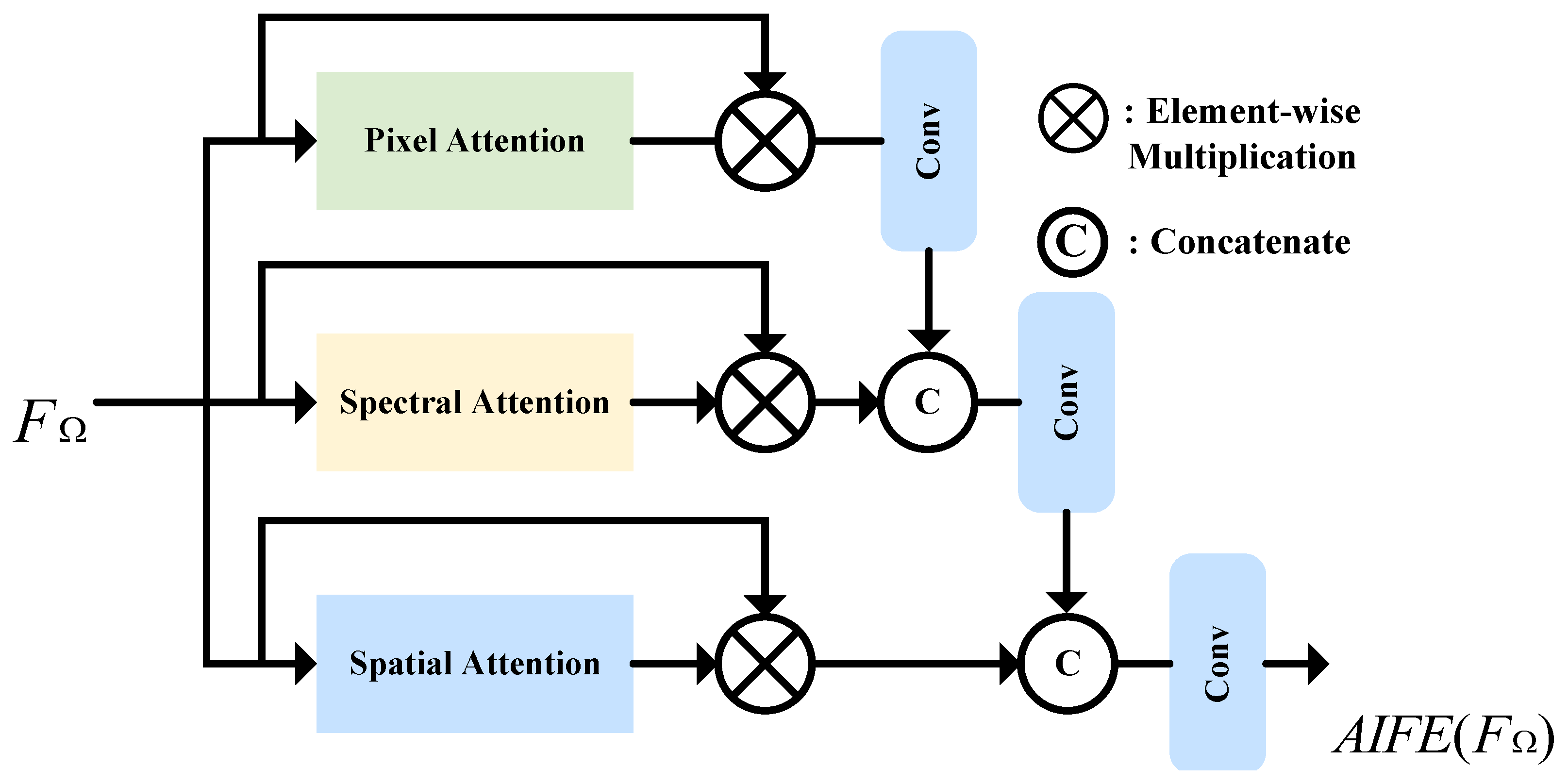
While the MLKC module effectively expands the receptive field and captures both local and nonlocal dependencies, it lacks the ability to perform adaptive modeling for specific spatial regions or spectral bands. This limitation may lead to the attenuation of fine structural details and suboptimal feature representation. To address this issue, we propose the AIFE module, which reconstructs multi-scale features along three dimensions (pixel, spectral, and spatial) to simultaneously enhance detail preservation and maintain global structural coherence. The AIFE module combines lightweight spectral and spatial attention with pixel-wise attention to selectively refine the fused representation across multiple dimensions. Specifically, the spectral and spatial attention mechanisms independently emphasize informative spectral patterns and spatial layouts, enabling the network to concentrate on semantically salient regions. Meanwhile, the pixel-wise attention branch further refines local detail representations such as edges and textures. The overall architecture of the AIFE module is illustrated in Figure 3.

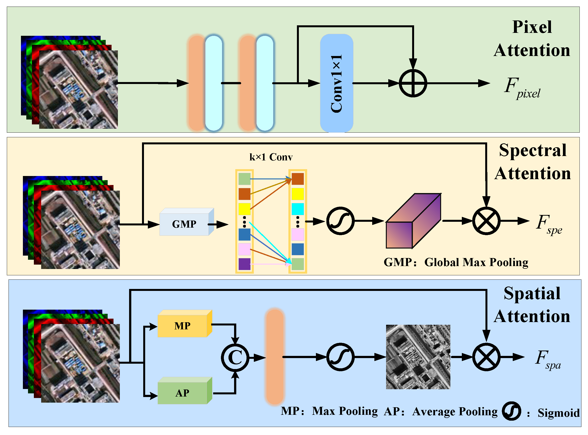
The detailed structures of the pixel attention, spectral attention, and spatial attention branches are shown in Figure 4. The pixel attention consists of sequential 3 × 3 convolution layers with ReLU activation, followed by a residual 1 × 1 convolution. The spectral attention path employs global max pooling (GMP) to squeeze spatial dimensions, followed by a 1D convolution and sigmoid activation to compute spectral attention weights. In contrast, the spatial attention branch combines max pooling (MP) and average pooling (AP) across the spectral channel, followed by a shared convolution and sigmoid activation to generate spatial attention maps. The computation process of AIFE can be formulated as follows:

$$\begin{array}{cc}\hfill F_{\mathrm{pixel}}& =F_{\Omega }\odot \sigma \left({Conv}_{1\times 1}\left(ReLU\left({Conv}_{3\times 3}\left(F_{\Omega }\right)\right)\right)\right)\hfill \\ \hfill F_{\mathrm{spe}}& =\sigma \left({Conv}_{1\times 1}\left(GMP\left(F_{\Omega }\right)\right)\right)\otimes F_{\Omega }\hfill \\ \hfill F_{\mathrm{spa}}& =\sigma \left({Conv}_{3\times 3}\left(Cat\left(MP\left(F_{\Omega }\right),AP\left(F_{\Omega }\right)\right)\right)\right)\otimes F_{\Omega }\hfill \end{array}$$

(10)

where $F_{\Omega }$ denotes the input feature map, $F_{\mathrm{pixel}}$ is the output of the pixel attention module, and $F_{\mathrm{spe}}$ and $F_{\mathrm{spa}}$ represent the results of the spectral and spatial attention modules, respectively. ⊕ denotes the concatenation operation.

3.6. Loss Function

After designing the network architecture, we use the mean squared error (MSE) as the loss function. The loss is defined by the following equation:

$$\begin{array}{c}\hfill \mathrm{Loss}={\displaystyle \frac{1}{N}}\sum _{i=1}^N{∥{\mathrm{GT}}_i-{\mathit{HRMS}}_{\mathit{i}}∥}^2\end{array}$$

(11)

where $\mathit{i}$ denotes the $\mathit{i}$-th training sample, N is the total number of training samples, and $HRMS$ represents the output result of the proposed network.

4. Experimental Results and Discussion

This section introduces the experimental settings in detail, including the datasets used, comparison methods, evaluation metrics, and implementation parameters. To comprehensively evaluate the performance of the proposed method, we conduct experiments on three widely used datasets and compare our results with several state-of-the-art methods. Additionally, ablation studies are performed to validate the contribution of each key module within our framework.

4.1. Experiment Setting

To assess the performance of the proposed CLNNet, experiments were conducted on three publicly accessible datasets from PanCollection [54], namely, WorldView-3 (WV3), GaoFen-2 (GF2), and QuickBird (QB). These datasets represent different sensors and scene characteristics. GF2 provides a PAN image with 0.8 m spatial resolution and a four-band MS image (blue, green, red, NIR) with 3.2 m spatial resolution. QB provides a PAN image at approximately 0.6 m resolution and a four-band MS image (blue, green, red, NIR) at approximately 2.4 m resolution. WV3 provides a PAN image at 0.4 m resolution and an eight-band MS image at 1.6 m resolution, enabling evaluation under richer spectral information. The detailed patch sizes and the numbers of training, validation, and testing samples are summarized in

Table 1. The basic information for each dataset.

Satellite	Spatial Resolution	Training		Validation		Testing
		Size	Number	Size	Number	Size	Number
WV3	1.6 m MS	16 × 16 × 8 MS	9714	16 × 16 × 8 MS	1080	64 × 64 × 8 MS	20
	0.4 m PAN	64 × 64 PAN		64 × 64 PAN		256 × 256 PAN
GF2	3.2 m MS	16 × 16 × 4 MS	19,809	16 × 16 × 4 MS	2201	64 × 64 × 4 MS	20
	0.8 m PAN	64 × 64 PAN		64 × 64 PAN		256 × 256 PAN
QB	2.4 m MS	16 × 16 × 4 MS	17,139	16 × 16 × 4 MS	1905	64 × 64 × 4 MS	20
	0.6 m PAN	64 × 64 PAN		64 × 64 PAN		256 × 256 PAN

. For evaluation, both reduced-scale and full-scale scenarios were considered. Since HRMS images are unavailable in the original satellite data, we follow Wald’s protocol [55] to generate simulated inputs and corresponding reference labels for training and testing.

To ensure a comprehensive evaluation, we compare the proposed method with several traditional and DL-based methods. For example, GSA [10] exemplifies CS-based fusion, while wavelet transform methods are typical of MRA-based methods. DL-based methods include PNN [21], MSDCNN [25], FusionNet [22], TDNet [26], AWFLN [35], SSCANet [36], PRNet [37], HEMSC [28], and IACDT [3]. The traditional methods were implemented using MATLAB 2017b. All DL-based pansharpening methods were implemented using Python 3.9 and PyTorch 2.4.1 on a rented server equipped with an NVIDIA GeForce RTX 4090D GPU. The training parameters for DL-based pansharpening methods were as follows: the Adam optimizer was used to update network parameters; the batch size was set to 32; the number of epochs was set to 300; and the initial learning rate was 0.0005, and it decayed by a factor of 0.8 every 100 epochs.

4.2. Evaluation Indicators

For objective evaluation, the fusion performance was quantitatively assessed using two strategies: reduced-scale and full-scale. In the reduced-scale experiments, the evaluation metrics included Spectral Angle Mapper (SAM) [56], Erreur Relative Globale Adimensionnelle de Synthèse (ERGAS) [57], correlation coefficient (CC) [58], the Universal Image Quality Index (Q) [59], and its extended version Q2n [60]. SAM measures the spectral angle between corresponding pixels in the fused image and the ground truth (GT), where lower values indicate less spectral distortion, with the ideal value being 0. ERGAS evaluates the overall spectral fidelity of the fused image; lower values suggest better spectral preservation, ideally approaching 0. CC reflects the geometric similarity between the fused and reference images, with higher values indicating better fusion quality. Q and Q2n are widely used image-quality indices in pansharpening, where values closer to 1 represent better visual and spectral performance. For the full-scale experiments, the evaluation metrics included Quality with No Reference (QNR) [61], the Spectral Distortion Index (D_λ), and the Spatial Distortion Index (D_s). D_λ and D_s evaluate spectral and spatial distortions, respectively; both are distortion-based metrics where lower values indicate higher quality, with the ideal value being 0. QNR is a composite no-reference index that combines D_λ and D_s to assess overall fusion quality, where a value closer to 1 denotes better performance.

4.3. Reduced-Scale Experiments

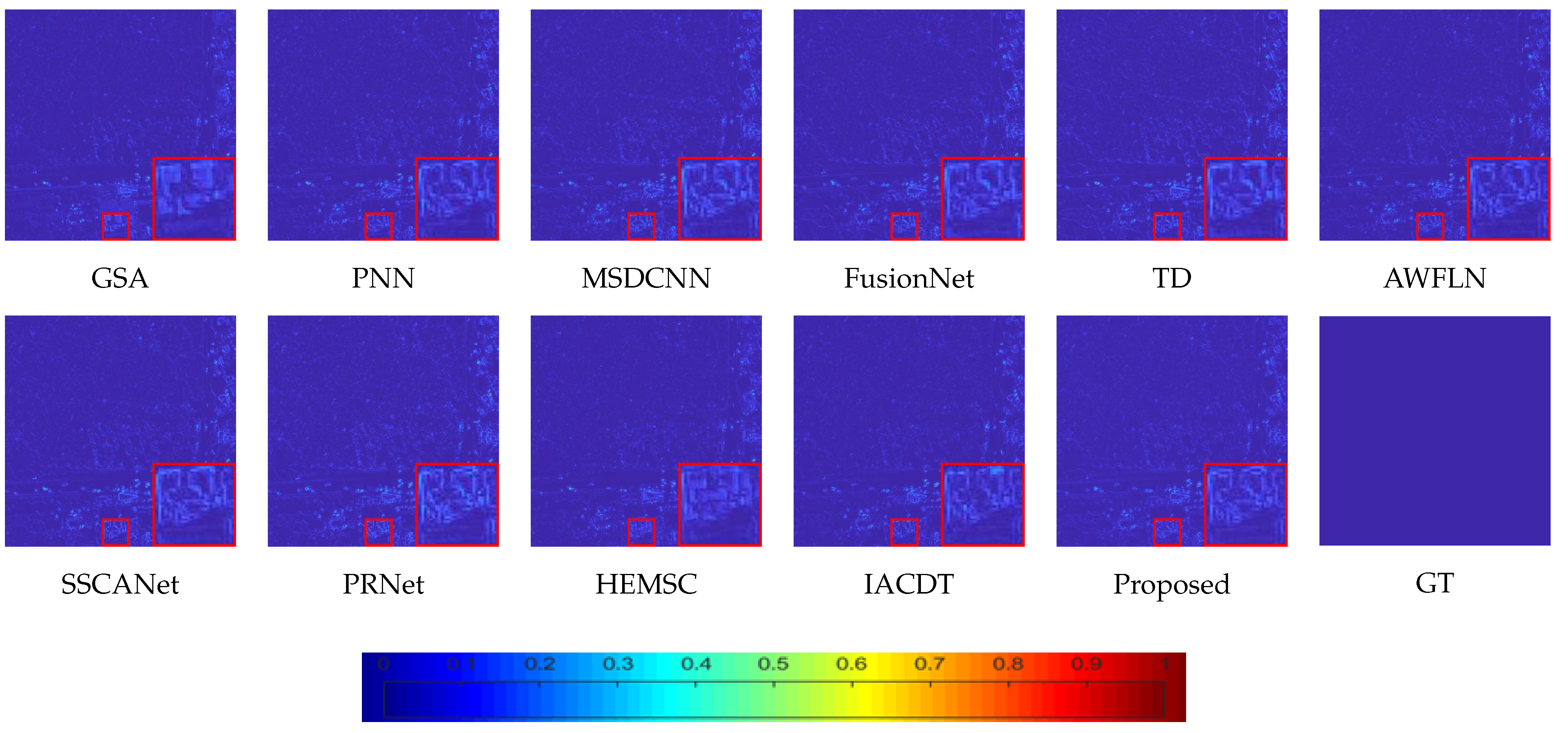
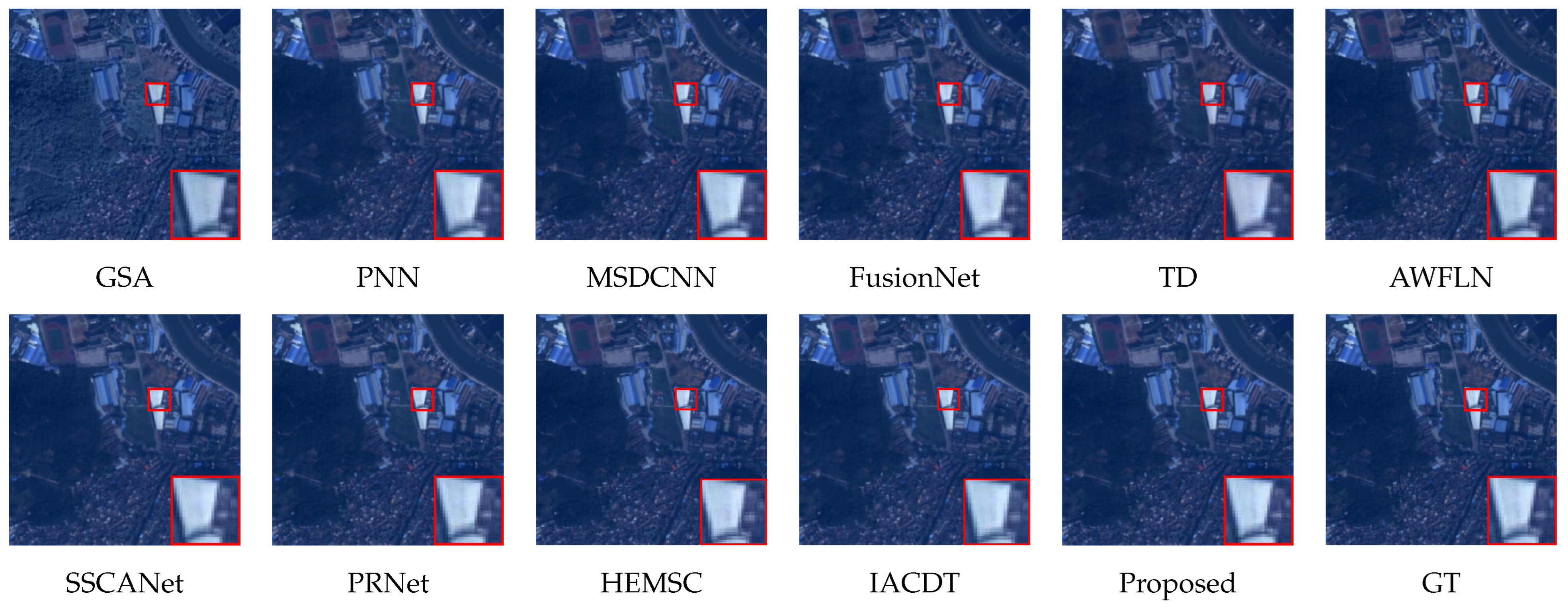
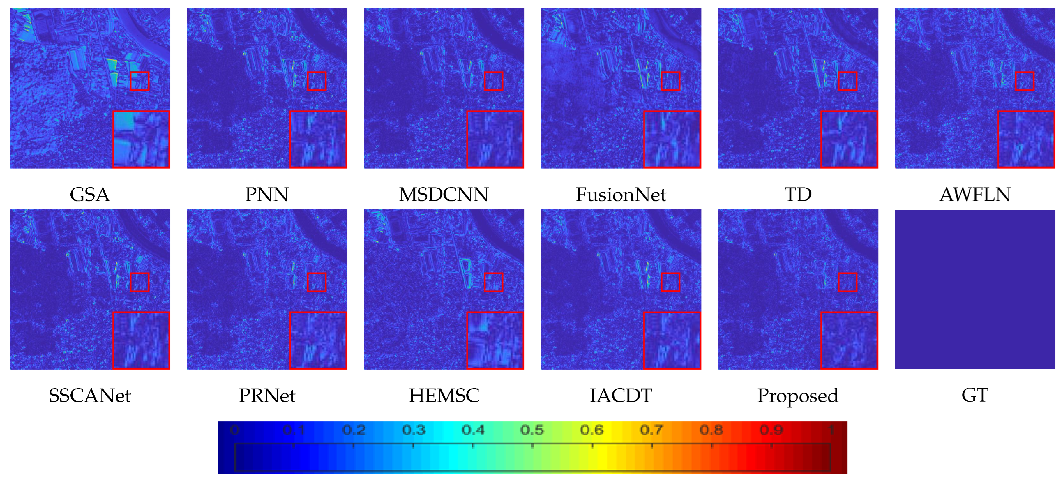
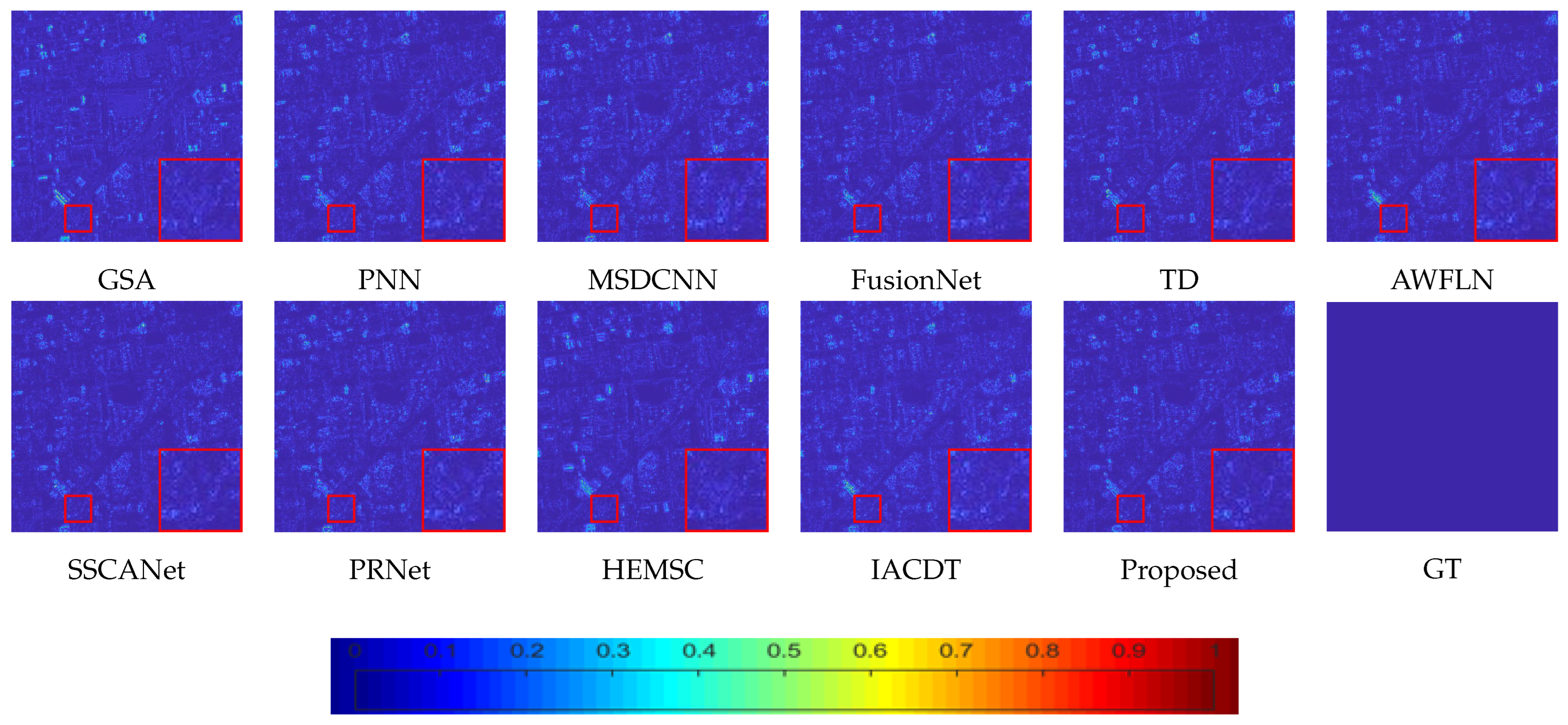
Reduced-scale experiments were conducted to demonstrate the effectiveness of CLNNet on the WorldView-3, GaoFen-2, and QuickBird datasets. The MS and PAN image patches were set to sizes of 16 × 16 and 64 × 64, respectively. For quantitative evaluation, the highest score of each metric is highlighted in bold to facilitate comparison among methods. For qualitative analysis, representative local regions of the fused results were enlarged to better reveal fine spatial details. Additionally, residual maps were employed to illustrate the similarity between the fused outputs and the ground truth (GT), where a higher proportion of blue areas indicates superior fusion quality.

Figure 5 illustrates the fusion results on the WV3 dataset, with only the RGB bands displayed to facilitate clearer visualization. The red rectangle marks the enlarged region corresponding to the highlighted area. As observed, the wavelet-based method suffers from severe spectral distortion caused by global color shifts. The outputs of PNN, FusionNet, and TDNet exhibit blurring, indicating insufficient spatial detail extraction. In contrast, AWFLN, PRNet, HEMSC, and CLNNet produce results visually closer to the GT, exhibiting only minor differences among them. The proposed method delivers fused images that exhibit the highest consistency with the GT. Residual maps [22] are shown in Figure 6 to further distinguish differences between the methods, clearly illustrating that the proposed method produces results closer to the GT.

Table 2. Quantitative evaluation of fusion results and quantitative evaluation on the WorldView-3 dataset. The best result in each group is in bold font.

Method	SAM	ERGAS	CC	Q	Q2n
Reference	0	0	1	1	1
GS	3.7059	3.7237	0.9440	0.9178	0.8701
PNN	3.2527	3.7676	0.9324	0.9346	0.9043
MSDCNN	3.1751	3.7563	0.9337	0.9391	0.9014
FusionNet	3.2027	3.8314	0.9299	0.9367	0.8938
TD	3.7612	4.0138	0.9222	0.9220	0.8887
AWFLN	3.0399	3.2799	0.9509	0.9455	0.9241
SSCANet	3.1215	3.6511	0.9342	0.9353	0.9091
PRNet	3.0431	3.5600	0.9407	0.9432	0.9095
HEMSC	3.0412	3.3251	0.9497	0.9448	0.9165
IACDT	2.9984	3.2883	0.9504	0.9476	0.9206
Proposed	2.8904	3.1167	0.9561	0.9510	0.9295

presents the quantitative evaluation results on the WV3 dataset. Overall, the DL-based methods outperform traditional ones, and the proposed method achieves the best scores across all metrics, confirming its superior performance and validating its effectiveness. On the WV3 dataset, CLNNet achieves a lower SAM than IACDT, indicating improved spectral angle preservation under the challenging 8-band setting. This phenomenon can be attributed to the complementary contributions of the two core modules. ACKC enhances local band-aware feature extraction by generating channel-specific kernels, which strengthens interband spectral correlations and suppresses band-dependent distortions; therefore, it directly benefits spectral-consistency-related metrics such as SAM. Meanwhile, MSLKA performs nonlocal modeling via large-kernel attention, which aggregates long-range cues and stabilizes global structures, reducing spatial inconsistencies that often introduce local spectral fluctuations at edges and textured regions.

The visualization results of the GF2 dataset under reduced resolution are shown in Figure 7. The fusion result produced by the GSA-based method exhibits the most severe spectral distortions. Compared to traditional methods, the DL-based methods demonstrate reduced spectral distortion. The residual maps in Figure 8 demonstrate that the proposed method produces fewer residuals. Overall, the proposed method demonstrates superior ability in preserving both spatial and spectral information.

Table 3. Quantitative evaluation of fusion results on the GaoFen-2 dataset. The best result in each group is in bold font.

Method	SAM	ERGAS	CC	Q	Q2n
Reference	0	0	1	1	1
GS	2.2910	2.7521	0.9638	0.9813	0.9834
PNN	1.2419	1.4149	0.9914	0.9951	0.9679
MSDCNN	1.1818	1.2264	0.9946	0.9957	0.9684
FusionNet	1.4876	2.0101	0.9837	0.9939	0.9414
TD	1.6121	1.7412	0.9869	0.9921	0.9537
AWFLN	1.0576	0.8940	0.9968	0.9965	0.9883
SSCANet	1.1074	1.1781	0.9959	0.9956	0.9726
PRNet	0.8819	0.8188	0.9971	0.9973	0.9891
HEMSC	0.9013	0.8372	0.9968	0.9967	0.9885
IACDT	0.8811	0.8993	0.9965	0.9972	0.9867
Proposed	0.8221	0.7297	0.9977	0.9977	0.9917

summarizes the evaluation metrics for the GF2 dataset under reduced resolution. Among traditional methods, the GSA and wavelet methods show relatively poor spatial and spectral fidelity due to their limited capability in modeling complex cross-band correlations and spatial detail compensation. This is reflected in their significantly higher SAM and ERGAS values compared with other methods, indicating larger spectral angle deviation and higher overall reconstruction error, respectively. Although the performance of DL-based methods is comparable, our proposed method achieves the best results across all reduced-resolution metrics because ACKC enhances local band-aware feature extraction to improve spectral consistency, while MSLKA provides long-range contextual aggregation to stabilize global structures and reduce spatial artifacts.

Figure 9 shows the fusion results for a pair of images from the QB dataset. In the magnified region marked by the red rectangle, several spatial details can be observed. Compared to the GT image, the results generated by SSCANet, AWFLN, and FusionNet appear noticeably darker. TDNet shows slight spectral distortion, whereas HEMSC produces images with evidently blurred edge textures. Figure 10 displays the residual maps, where the residual values among the DL-based methods are relatively similar.

Table 4. Quantitative evaluation of fusion results on the QuickBird dataset. The best result in each group is in bold font.

Method	SAM	ERGAS	CC	Q	Q2n
Reference	0	0	1	1	1
GS	7.9179	9.4878	0.9106	0.7998	0.7838
PNN	5.8779	6.6128	0.9321	0.8676	0.9235
MSDCNN	5.6568	6.2754	0.9400	0.8760	0.9324
FusionNet	5.6995	6.4534	0.9388	0.8750	0.9303
TD	7.0817	8.1985	0.8949	0.8150	0.8843
AWFLN	5.4978	6.2451	0.9401	0.8824	0.9317
SSCANet	5.5819	6.1264	0.9422	0.8787	0.9348
PRNet	5.4904	6.1631	0.9417	0.8818	0.9351
HEMSC	5.4963	6.2143	0.9405	0.8826	0.9329
IACDT	5.3993	6.0121	0.9470	0.8910	0.9350
Proposed	5.3539	5.9193	0.9475	0.8898	0.9370

lists the evaluation metrics for the QB dataset under reduced resolution. Our proposed method outperforms all others across all reduced-resolution metrics, achieving particularly significant improvements in SAM and ERGAS.

Different land-cover types can affect pansharpening difficulty due to scene-dependent textures and spectral mixing. The experimental results demonstrate that CLNNet mitigates this variability via progressive local–nonlocal refinement and consistently achieves lower SAM across heterogeneous scenes, indicating improved spectral preservation. Nevertheless, performance may still vary under extreme scene distributions, and improving cross-domain generalization will be explored in future work.

4.4. Full-Scale Experiments

We evaluate all comparison methods on the full-resolution dataset, where PAN/LRMS have the original size of 512 × 512/128 × 128.

Table 5. Quantitative assessment indicators for full-scale experiments. The best result in each group is in bold font.

	WorldView-3			GaoFen-2			QuickBird
Method	QNR	Dλ	${\mathbf{D}}_{\mathbf{s}}$	QNR	Dλ	${\mathbf{D}}_{\mathbf{s}}$	QNR	Dλ	${\mathbf{D}}_{\mathbf{s}}$
Reference	1	0	0	1	0	0	1	0	0
GS	0.8730	0.0232	0.1063	0.7471	0.1094	0.1612	0.6781	0.0610	0.2778
PNN	0.9389	0.0184	0.0435	0.9239	0.0384	0.0393	0.8906	0.0225	0.0889
MSDCNN	0.9497	0.0124	0.0384	0.9132	0.0445	0.0443	0.8836	0.0352	0.0842
FusionNet	0.9477	0.0194	0.0336	0.8143	0.1282	0.0659	0.8526	0.0745	0.0788
TD	0.8615	0.0526	0.0907	0.8738	0.0602	0.0703	0.7358	0.0967	0.1854
AWFLN	0.9493	0.0207	0.0316	0.9605	0.0219	0.0180	0.9134	0.0243	0.0639
SSCANet	0.9285	0.0147	0.0576	0.8950	0.0525	0.0554	0.8516	0.0147	0.1357
PRNet	0.9609	0.0165	0.0229	0.9433	0.0317	0.0258	0.9162	0.0233	0.0620
HEMSC	0.9587	0.0189	0.0288	0.9596	0.0256	0.0152	0.9142	0.0238	0.0636
IACDT	0.9656	0.0162	0.0185	0.9470	0.0332	0.0206	0.9157	0.0242	0.0615
Proposed	0.9679	0.0103	0.0221	0.9609	0.0219	0.0176	0.9196	0.0210	0.0607

reports the values of no-reference full-scale evaluation metrics on the WV3, GF2, and QB datasets. The GSA and wavelet methods exhibit relatively poor QNR scores, whereas the DL-based methods consistently outperform the traditional methods in terms of overall performance metrics. As shown in Table 5, our proposed method achieves the best performance in terms of QNR and Ds on the WV3 dataset in the full-scale experiments, highlighting its strength in maintaining spectral consistency and enhancing spatial resolution. In general, compared with both the traditional and existing DL-based methods, the proposed method consistently achieves superior fusion results across all three datasets (WV3, GF2, and QB), further confirming its generalizability and effectiveness.

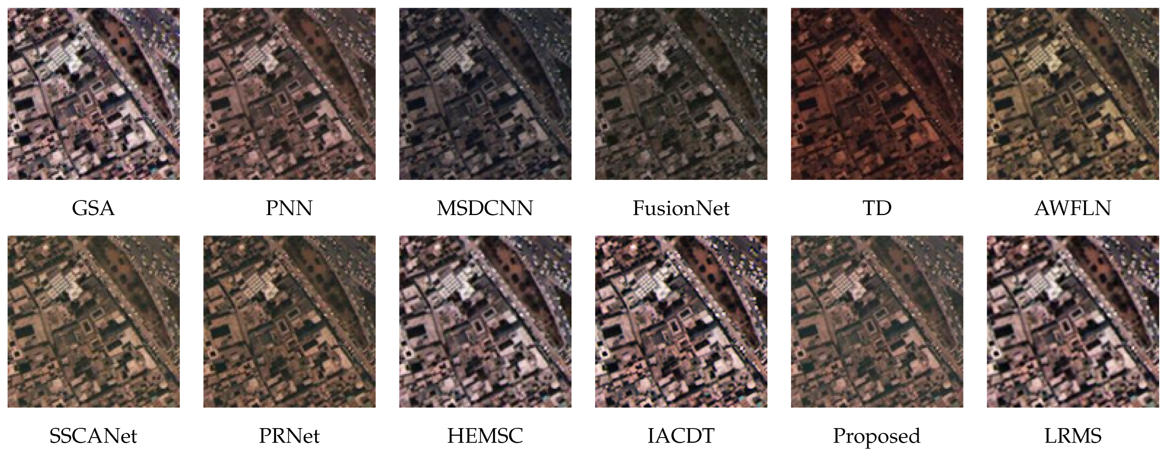
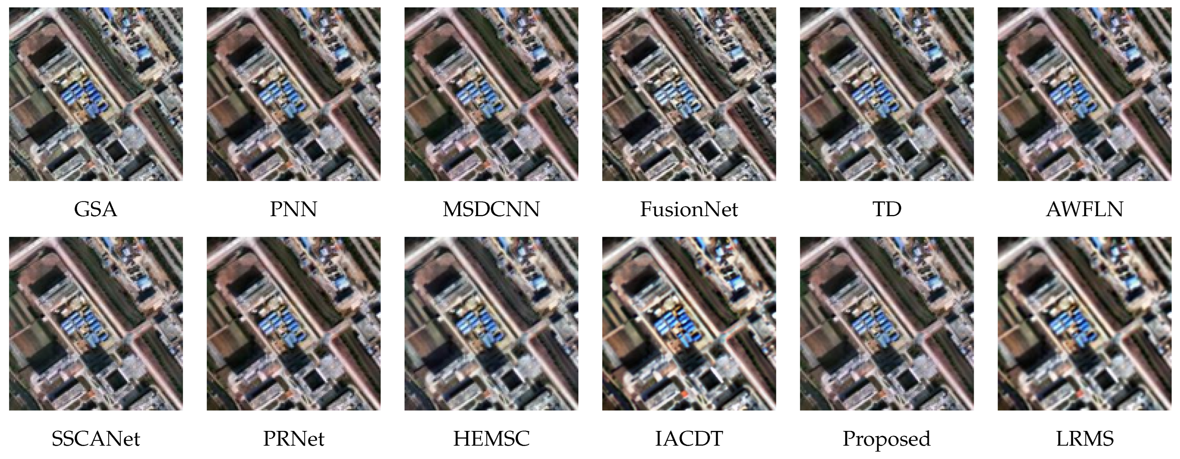
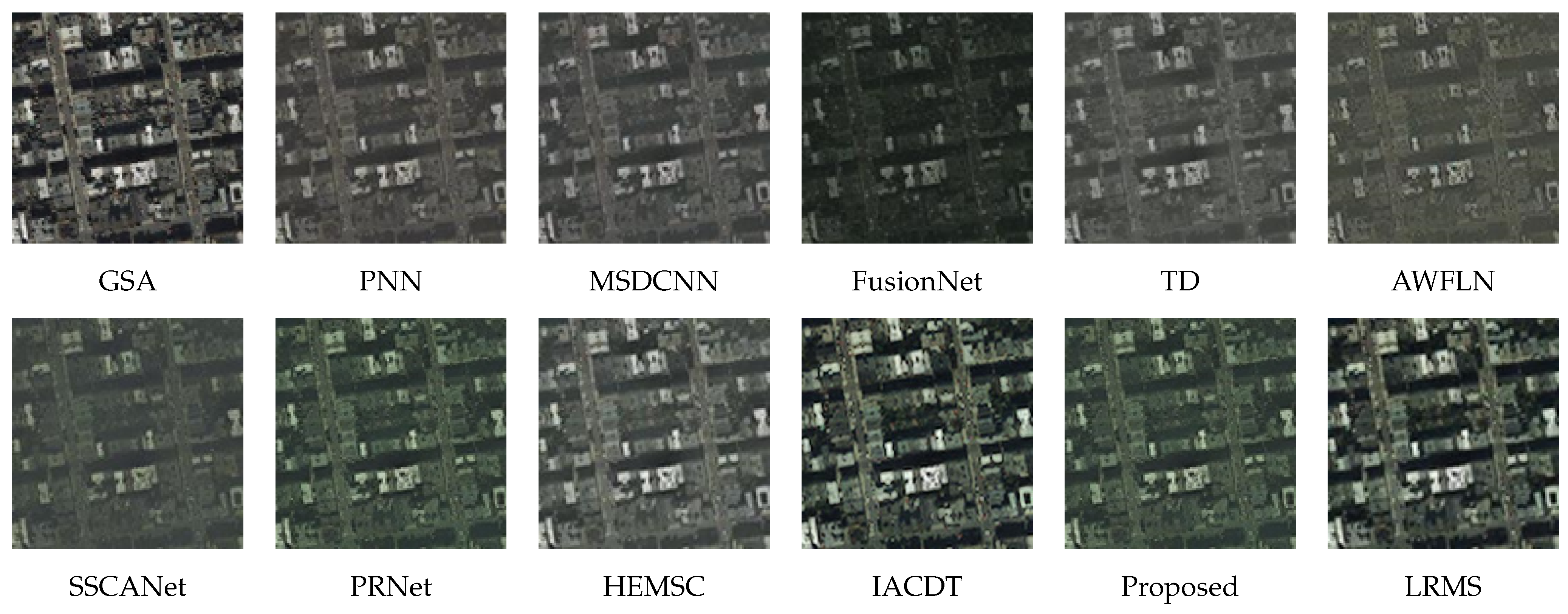
Figure 11, Figure 12 and Figure 13 present the full-scale fusion results on the WV3, GF2, and QB datasets, respectively. The visual differences in spatial and spectral quality among the methods can be clearly observed. In Figure 11, the traditional wavelet method shows evident spectral distortions, manifested as noticeable color shifts, indicating its limited capability in reconstructing high-resolution spectral content. Figure 12 shows the results on the GF2 dataset, where some DL-based methods are less effective in recovering spatial details compared to our method-particularly in terms of edge structure and texture clarity. This observation is also reflected in the quantitative metrics for the GF2 dataset shown in the table. In Figure 13, which corresponds to the QB dataset, traditional methods such as GSA and wavelet display apparent spectral distortions. In contrast, PRNet, HEMSC, and our proposed method demonstrate significantly higher resolution and clarity in the fused images. Due to the absence of ground-truth images, distinguishing performance differences is challenging. Nevertheless, as shown in Table 5, the proposed method demonstrates overall superiority compared with the other methods.

4.5. Discussion

To understand the performance gains, we analyze the key structural differences between CLNNet and existing pansharpening models. CLNNet incorporates three major design changes that contribute to improved accuracy. First, a progressive multi-stage backbone enables iterative refinement, reducing error accumulation compared with one-shot fusion strategies. Second, channel-specific adaptive kernel convolution with global contextual enhancement supports band-aware local feature modeling, which suppresses band-dependent intensity drift and improves spectral fidelity. Third, multi-scale large-kernel attention aggregates nonlocal contextual information after local extraction, capturing long-range dependencies and reducing edge blurring in heterogeneous regions. These structural advantages are consistent with the observed improvements in both quantitative metrics and visual quality.

4.6. Ablation Study

To further validate the effectiveness and contributions of different components in the proposed CLNNet, we conducted a series of ablation experiments on the GF2 dataset. By systematically removing or simplifying specific modules within the network and evaluating the performance using quantitative metrics, we aimed to assess the role each module plays in enhancing fusion quality.

The full model consists of three key components: the data preprocessing module, the ACKC module, and the MSLKA module. ACKC and MSLKA jointly form the core feature extraction unit, which is stacked in three layers in the main network backbone, accompanied by residual connections to enhance deep feature learning capability. We designed the following five ablation scenarios: in case 1, retaining only the MSLKA module without ACKC led to a notable increase in the SAM and ERGAS values, and the fused images exhibited blurry textures and indistinct edge structures, which demonstrates the importance of ACKC for modeling local fine-grained features. In case 2, we replaced the proposed preprocessing stage with a conventional interpolation-based upsampling scheme, i.e., using traditional interpolative upsampling instead of our dual-branch design. In case 3, the MSLKA module was removed while retaining the ACKC for feature modeling, the results demonstrated a significant deterioration in both spatial and spectral quality of the fused images, as reflected by the decline in multiple evaluation metrics. This highlights the critical role of MSLKA in maintaining global structural consistency. In case 4, to investigate the impact of network depth, the number of stacked ACKC and MSLKA units was reduced from three to two layers. Although this made the model more lightweight, its ability to preserve fine details and structural consistency weakened noticeably, with quantitative metrics showing clear degradation, thereby supporting the advantage of the original three-layer design. In case 5, to assess the effectiveness of the proposed sequential local-to-nonlocal design, a parallel variant was constructed in which the ACKC and MSLKA modules operate concurrently rather than cascaded; specifically, local and nonlocal features extracted by ACKC and MSLKA were combined by element-wise addition. While this parallel structure maintained a comparable number of parameters, its performance declined significantly, confirming the superiority of the cascaded design. In case 6, both the ACKC and MSLKA modules were replaced with standard convolutional layers, thereby removing all adaptive and attention mechanisms, resulting in a substantial performance drop across all evaluation metrics, with fused images suffering from pronounced spatial and spectral distortions. This confirms the necessity of the proposed modules for building a high-performance fusion network. Case 7 is our proposed CLNNet method.

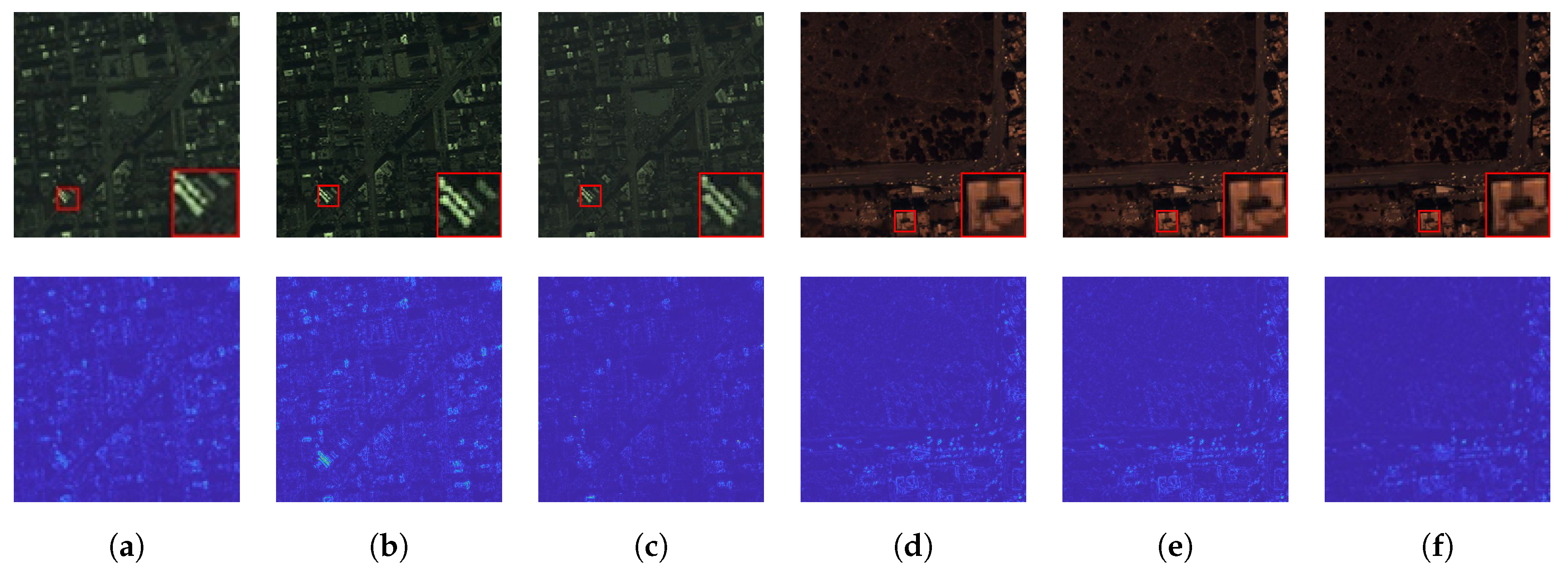
Figure 14 presents the visual results of selected experiments, while

Table 6. Comparison of quantitative assessment of ablation experiments on the GaoFen-2 dataset. The best result in each group is in bold font.

Case	ACKC	MSLKA	Traditional Upsampling	Three Layers	Parallel	SAM	ERGAS	CC	Q	Q2n
1		✓		✓		0.9707	0.8735	0.9968	0.9974	0.9895
2	✓	✓	✓	✓		0.8979	0.9632	0.9959	0.9971	0.9848
3	✓			✓		1.0272	1.0039	0.9956	0.9964	0.9835
4	✓	✓				0.9783	0.8988	0.9965	0.9967	0.9867
5	Conv	Conv		✓		0.9235	0.8414	0.9970	0.9971	0.9887
6	✓	✓		✓	✓	0.9166	0.7950	0.9974	0.9972	0.9902
7	✓	✓		✓		0.8221	0.7297	0.9977	0.9977	0.9917

summarizes the average quantitative metrics. The results demonstrate that each proposed module contributes positively to the overall fusion quality, validating the effectiveness and rationality of the network design.

To verify the generalization of our core modules under different spectral dimensions and imaging conditions, we further conducted ablation studies on the QB and WV3 datasets.

Table 7. Comparison of quantitative assessment of ablation experiments on the QB and WV3 datasets (core modules). The best result in each group is in bold font.

Case	ACKC	MSLKA	SAM	ERGAS	CC	Q	Q2n
1		✓	5.8419	6.1515	0.9287	0.8870	0.9243
2	✓		6.1301	8.0240	0.9017	0.8562	0.8939
3	✓	✓	5.3539	5.9193	0.9475	0.8898	0.9370
4		✓	3.1343	3.6850	0.9354	0.9394	0.9040
5	✓		3.3225	3.9270	0.9136	0.9160	0.8896
6	✓	✓	2.8904	3.1167	0.9561	0.9510	0.9265

summarizes the quantitative metrics. In Figure 15, case 1–case 3 are performed on the QB dataset, and case 4–case 6 are performed on the WV3 dataset. In case 1 and case 4, we remove ACKC from the network. In case 2 and case 5, we remove MSLKA. Case 3 and case 6 correspond to the full proposed model with all modules enabled.

4.7. Limitations in Remote Sensing Applications

Our experiments mainly use cloud-free images. Thin clouds and haze may introduce spatially varying attenuation and spectral bias, which can reduce the reliability of pansharpening results. In addition, different satellite sensors may have different radiometric responses and imaging characteristics, and the performance may vary when transferring the model across sensors without adaptation. Finally, some practical applications require fast processing with limited computing resources; future work will explore lightweight designs, including a more compact network and model compression methods to reduce computational cost while maintaining fusion quality.

5. Conclusions

Current pansharpening methods often fail to preserve local textures and overlook spectral correlations across bands when modeling nonlocal information in source images. To address these limitations, we propose a novel pansharpening network named CLNNet. The network incorporates an ACKC module that generates channel-specific convolution kernels for each channel. This design effectively enhances the model’s ability to capture local details from the PAN image and strengthen the feature correlations among different spectral bands in the HRMS image. Moreover, we design an MSLKA module that leverages LKCs to obtain long-range dependencies. It further integrates pixel, spectral, and spatial attention mechanisms to improve structural continuity, spectral consistency, and feature complementarity. Comparative experiments conducted on multiple remote sensing datasets demonstrate that our method outperforms other conventional and state-of-the-art methods. Furthermore, the ablation studies confirm the effectiveness and collaboration of the ACKC and MSLKA modules within the proposed architecture. Future work will explore the use of frequency-domain information and multi-scale features to further enhance both the structural continuity and spectral consistency of pansharpening.