An Algorithm for Extracting Bathymetry from ICESat-2 Data That Employs Structure and Density Using Concentric Ellipses

Highlights

What are the main findings?

• High accuracy was achieved from a novel algorithm for extracting bathymetric photon events (PEs) from ICESat-2 data using PE spatial structure as well as more conventional density.
• Across three global datasets the algorithm appears to be sufficiently robust to not require local tuning.

What are the implications of the main findings?

• The high accuracy identification of bathymetric PEs may improve the accuracy of satellite derived bathymetry that uses the bathymetric PEs for training.
• The method’s robustness may provide improved efficiency in reducing the amount of manual effort required to identify bathymetric PEs in ICESat-2 tracks.

Abstract

The ICESat-2 satellite collects LiDAR data along linear orbital tracks using a photon-counting green wavelength (532.27 nm) instrument. The utility of combining ICESat-2 data with satellite imagery for training and subsequently applying satellite-derived bathymetry models to provide estimates of shallow water depth is well-established. However, automating and improving the accuracy of the identification of ICESat-2 photon events (PEs) representing bathymetry remains a challenge. This article presents an algorithm for automated extraction of PEs reflected from the ocean floor (rather than the ocean surface or noise in the water column). The algorithm is unique in examining both the density of PEs surrounding a subject PE and their position relative to the subject PE. This is accomplished by establishing three concentric ellipses around the subject PE, dividing them into radial “sectors” in 2D space (along-track vs. PE depth/height), recording the number of neighboring PEs in each sector and using this information to fit a LightGBM model. Agreement with PEs identified by an image interpreter is approximately 98%. Testing suggests that the accuracy of the algorithm is relatively insensitive to the size and shape of the ellipses used to define a PE’s neighborhood and to the number of radial sectors used. The model produced also appears to be robust across different geographic areas and data densities.

1. Introduction

The Ice, Cloud, and land Elevation Satellite-2 (ICESat-2) satellite was launched in October 2018 for the purpose of cryosphere monitoring [1]. It is the successor to the initial ICESat satellite that was operational from 2003 to 2009. Since its launch, the use of ICESat-2 data has expanded beyond cryosphere monitoring to a number of application areas including shallow water bathymetric mapping—the subject of this article. This is made possible by ICESat-2’s data capture instrument—the photon-counting Advanced Topographic Laser Altimeter System (ATLAS). Because the ATLAS includes a green laser with a wavelength of 532.27 nm and a sensor that detects and counts reflected photons, the ATLAS can penetrate to depths shallower than 40 m, although penetration to deeper depths has been reported [2]. This is comparable to the generally reported depth penetration of airborne green lasers, although a depth penetration of airborne lidar of up to 75 m has been reported [3]. Despite the very low percentage of photons reflected from the sea bottom (as opposed to the water surface or atmospheric and water column noise) and subsequently detected by the ATLAS’ beryllium telescope, the data recorded are sufficiently numerous to obtain estimates of “shallow water” bathymetry, broadly defined here as depths less than 40 m. (Detected returned photons are referred to as “photon events” (PEs). For additional information about ICESat-2, see also [1,4]).

ICESat-2 data are collected in linear tracks—not pixels or areas—with a repeat cycle of 91 days. Because Earth cryosphere monitoring was the goal of the ICESat-2 mission, it was planned that the same orbit path would be followed repetitively. However, the ICESat-2 satellite is pointable which has led to deviations from the original plan. A single pass of ICESat-2 collects data from six tracks configured as three “beam pairs” separated by 3.2 km with each beam pair comprising two beams separated by 90 m. In each pair, there is a “strong” and a “weak” beam with the strong beam emitting four times the energy of the weak beam. (The original goal of this paired configuration was to be able to estimate terrestrial slope). The result is a nominal along-track spacing of 0.7 m between successive PEs on the strong beam and of 2.8 m along the weak beam. ICESat-2 data are delivered as 20+ “products”—many of which summarize PEs in “segments” of various sizes due to data volumes—that result from post-processing. The product employed in this study—as it is for most bathymetric applications—is “ATL03—Global Geolocated Photon Data”, specifically the {x, y, z} tuple that provides the location of each reflected PE collected by the ATLAS in three dimensions. For a more comprehensive understanding of the contents of the ATL03 product, readers are referred to the extensive ATL03 data dictionary [5] and associated ATL03 Algorithm Theoretical Basis Document [6].

To estimate shallow ocean depth using a satellite-derived bathymetry (SDB) approach, PEs that are reflected from the ocean bottom must be identified and a satellite image that best covers the geographic region of interest, accords with the date of the ICESat-2 data and has little or no cloud cover must be obtained. Depths of PEs representing ocean depth are then used to train an SDB model that empirically relates ocean depth to multi-band pixel reflectance. This is then applied over the entire image area to estimate shallow water depth.

A recent review article [7] characterized five approaches to identify optimal ways of extracting bathymetric data from ICESat-2 tracks for use in training. (Each also implicitly includes an initial step of eliminating water surface PEs):

• Density-based approaches assume that bathymetric PEs will be more closely spaced than noise PEs. Recent examples cited include [8,9].
• Median-filtering approaches assume that the densest region of PEs defines an area of bathymetric PEs. Examples include [10,11].
• Histogram-based approaches that share a commonality with waveform lidar methods by analyzing the histogram of PE depths. Examples include [12,13].
• Grid-based methods that analyze patterns after restructuring a PE cloud into grids. Examples include [14,15].
• Machine-learning-based methods that comprise a variety of methods having different underlying approaches to data analysis. Examples include [16,17].

As point-based (albeit with a footprint of ~11 m [18]) data collected along linear tracks, ICESat-2 data are two-dimensional (Figure 1). It is relatively straightforward to algorithmically filter out water surface PEs due to their comparatively high density (e.g., [13,15,19]). Similarly, various methods have been described to eliminate sparse atmospheric noise PEs based on their height and density (e.g., [20,21]). Hence the primary difficulty in using ICESat-2 data in an SDB process flow is that a large proportion of the below-surface PEs are water column noise rather than bathymetry. Algorithmically identifying bathymetric PEs with the same accuracy as manual image interpreters remains challenging. Because of the potential time- and cost-savings of automated bathymetric PE extraction, however, considerable effort continues to be expended on this topic. Indeed, a recent review article [7] cites approximately 100 articles published since 2021 that address this subject. Readers interested in previous work on extraction of bathymetry from ICESat-2 data are referred to this comprehensive review.

A large number of the approaches explored—indeed, potentially all of them—rely on along-track PE density. This is reasonable given that visual examination of Figure 1 would suggest that this is the main criterion on which image interpreters would base their interpretation. However, image interpreters would additionally base their interpretation on what we broadly refer to as “structure” that can adapt for characteristics such as changing PE densities and relative PE positions. Based on the review article by Jung et al. [7], PE structure—the relative positions of PEs—has received little attention for denoising ICESat-2 data, although there are exceptions. For example, grid-based approaches to ICESat-2 denoising that consider structure have been described—e.g., [22,23]. Similarly, three-dimensional grid-based approaches that employ “voxels” have been examined for denoising acoustic sonar data—e.g., [24].

Nonetheless, the use of non-grid structures to denoise ICESat-2 data for bathymetry has received little attention. The goal of this article is to present and evaluate the accuracy of an algorithm that has been developed to identify bathymetric PEs in ICESat-2 tracks. The algorithm is novel in that it enables expansion of density-based algorithms to also include spatial structure of PEs.

2. Materials and Methods

2.1. Algorithm and Description

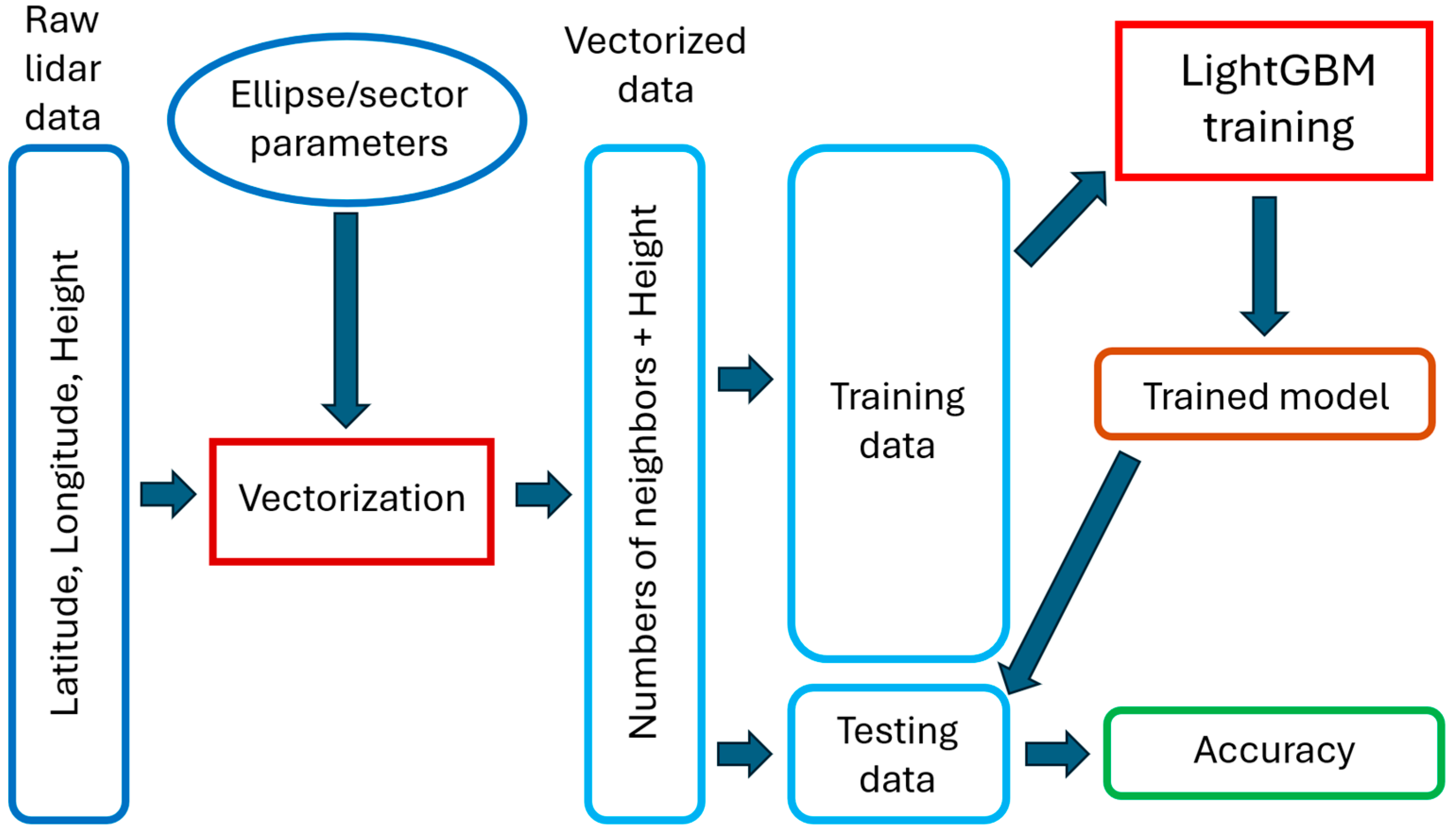
To facilitate reader comprehension, Figure 2 provides a visual representation of the algorithm modeling flow. We note that not represented in Figure 2 is the initial elimination of cloud-impacted segments. These were excluded from the model training and the classification processes subsequently described since no photons could reach the seafloor or even the water surface where clouds were present. Internal analysis of water surface variability within individual segments (a Gaussian distribution around the best estimate of the average water level was assumed) demonstrated that wave heights varied from almost zero to ~3 m. This, however, did not affect the training or classification as the proposed algorithm excluded PEs near the mean water level from consideration. Poor water clarity plays a role similar to clouds by not allowing photons to reach the seafloor. Because such segments were of no value for the algorithm, the segments within which fewer than 5% of total PEs were below surface PEs were also not considered.

Most of the algorithms proposed for extraction of shallow bathymetry from the ICESat-2 ATL03 product are based on detection of locally dense constellations of PEs [6]; examples are [23,24]. However, structure—the mutual positioning of neighboring PEs—is also important beyond the rigid structure of a grid-based approach. This was recognized and explored by Meng et al. [25]. To address the local structure of PEs, they defined the neighborhood of a PE as a single horizontal ellipse of pre-determined length and height centered on the PE. For a given PE, all neighbors within the ellipse were extracted, distances between each PE pair within the neighborhood calculated and a K-average nearest neighbor feature vector constructed; this was performed for all PEs in an ICESat-2 track. Using a training set of manually extracted bathymetric PEs, they then fitted and evaluated a back propagation neural network model to predict if unknown PEs represented bathymetry. Notably, their work did not consider the relative position of PEs within a subject PE’s neighborhood. Moreover, their effort focused on separating noise PEs from signal PEs without distinguishing between ocean surface and ocean bottom (i.e., bathymetry) signal PEs. This is consistent with the definition of “signal confidence” reported as the ICESat-2 attribute signal_conf_ph for each PE in ATL 03.

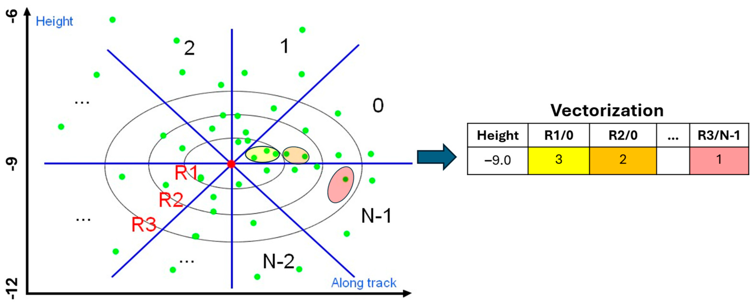
The algorithm developed herein proposes an alternative method to construct a density-structure feature vector that considers neighborhood structure and that can also be used in machine learning (ML) modeling to separate noise from bathymetric PEs. It first defines three elliptical neighborhoods (denoted by R1, R2 and R3 in Figure 3) around a subject PE. Though the number of ellipses is not fixed, three are employed here because a larger number resulted in an associated increased CPU time cost with little change to accuracy, as will be demonstrated subsequently. These ellipses are further sub-divided into “radial sectors” defined by the blue lines in Figure 3 and labeled from 0 to N − 1. The number of PEs in each radial sector is counted and recorded in a PE’s feature vector. The analytical rationale for this vectorization is that in an area of water column noise, neighboring PEs will be distributed roughly equally across all radial sectors. However, for both water surface and bathymetric PEs, the neighbors of each PE will be most common in the radial sectors closest to horizontal given that shallow water ocean floor slopes are generally not steep. Notably, even if a steep slope is present, results indicated that this ellipse-based approach still produces a useful structure description. Note that in addition to structure, this vectorization also characterizes information about the local density of PEs.

During development, it was observed that the density and structure of water surface and bathymetric PEs were similar. Hence PE height (the term “height” rather than “depth” is employed throughout since depth can simply be considered a negative height relative to some datum that in this case is mean sea level (MSL)) was added to each PE’s feature vector which allowed water surface PEs to be distinguished from bathymetric PEs. Note that a PE’s height is the only non-relative element of the resulting vector; its inclusion in the feature vector was determined to be essential for the proposed algorithm performance, as without height PEs representing the water surface were consistently classified as bathymetric. Notably, because ICESat-2 tracks and consequent segments were collected at different times, orthometric height of the water surface was not constant primarily due to tidal fluctuations. It is acknowledged that this could affect the accuracy of the proposed algorithm.

To overcome this, the water surface of each segment was estimated using a segmented histogram-based algorithm comparable to what is described in [26,27]. The algorithm comprises two steps. First the mode of the PE heights is identified on the assumption that this will be “near” the ocean surface height. Second, PEs with a height within 3 m of the “full distribution” modal value are retained. A Gaussian function is then fitted to the frequency distribution of this “refined” dataset and its peak identified. This peak produces a relatively accurate estimate of water level height. (The standard deviation of the refined dataset also provides an estimate of wave height). This approach ultimately provides an offset for each segment of an ICESat-2 track that allows PEs in each segment to be shifted vertically by a constant amount so that water surface has a height of 0 across all segments and tracks. Note that this does not affect the ellipse-based vectorization as the vectorization relies only on relative position which does not change through the application of a vertical constant. Further, note that this is not a tide correction that would have to be applied to PE heights for use in nautical charts.

Conceptually, this vectorization defines a local neighborhood for, and conveys information about, the local density of PEs while also recording within-sector PE counts that describe internal structure via their mutual orientation. Ellipses were chosen to define local neighborhoods, rather than circles, because in ICESat-2 tracks the horizontal scale of the PE distribution is considerably larger than the vertical scale. This reflects the topography of the shallow water sea bottom that is predominantly flat with rarely occurring steep slopes. Investigation of the optimal number of ellipses, their lengths, heights and shapes, and of the number of sectors demonstrated that the proposed algorithm resulted in almost identical outcomes for a wide range of parameters. These ranges will be discussed later with a demonstration of how their choice affected classification results. Consequently, except where noted, the following parameters were employed in this study: three ellipses with horizontal (major) axis radii of 2, 4 and 6 m, an aspect ratio of axes of 10 (i.e., the length of the horizontal radii are 10 times that of the vertical radii) and 12 radial sectors.

In addition to the vectorization of all PEs, training data identifying a PE as bathymetry or not (“Bathy” or “NotBathy”) are required to train a model that estimates the probability that a PE is Bathy using the PE feature vector as the predictor. In this study, training (and testing) datasets were developed through manual examination of ICESat-2 tracks. For model fitting, the machine learning algorithm LightGBM [28] was employed. Developed by Microsoft^® in 2016, a C++ implementation with Python (version 3.11) bindings is available. Advantages of LightGBM include effective prevention of model overfitting and early stopping that decreases computation time. For model fitting and use, PEs within 12 m (i.e., the largest ellipse length) of the end of a track were not used in model development or subsequent evaluation.

2.2. Data and Algorithm Analysis

The algorithm was developed and its performance explored over a wide geographic range that also represented a range of data conditions, e.g., densities, depths, etc. For these purposes, three datasets were employed:

• Five ICESat-2 “granules” (1/14 of an orbit) recorded in 2018 around the Florida Keys (United States) region centered approximately on 24.60°N/81.50°W (lat/lon).
• The dataset employed by Lin and Knudby [16] comprised 40 globally distributed ICESat-2 granules collected in 2018 and identified as containing Bathy PEs using the OpenAltimetry platform [29].
• A publicly available globally distributed dataset stored in the Scholars Archive at the Oregon State University [30].

For the first dataset centered on Key West (FL, USA; subsequently referred to as the “KW” dataset), the appropriate ICESat-2 granules were downloaded from the United States National Snow and Ice Data Center, (NSIDC, date unknown (a)) from their respective sources. Each granule was divided into segments containing 32,678 PEs; this typically corresponded to a length of 10 to 12 km. Segments having 5% or more of their PEs below the water surface (the zero orthometric level) were retained for analysis. Each segment was inspected manually using JMP software (Student edition, version 18.2.1), and the PEs identified as Bathy were marked as such; the other PEs in each segment were marked as NotBathy. This annotation served as the “ground-truth”/reference data for model training and evaluation.

The Lin and Knudby and OSU datasets (subsequently referred to as the “L&K” and “OSU” datasets, respectively) were downloaded from their respective repositories. Each consisted of granules that had already been divided into segments of roughly equal size. Individual PEs had been manually identified as Bathy or NotBathy by the creators of those datasets and were provided with those datasets.

These data are summarized in

Table 1. Description of datasets.

Name	Region	Year	Approx. Lat/Lon Center	Number of ICESat-2 Granules	Number of Segments	Total PEs	NotBathy PEs	Bathy PEs
Key West (“KW”)	Florida Keys	2019	24.60°N 81.50°W	5	452	14,452,515	11,192,179	3,260,336
Lin and Knudby (“L&K”)	Global	2018	Varies	40	96	3,001,664	2,478,148	523,516
OSU (“OSU”)	Global	2019–2022	Varies	Varies	101	6,768,540	6,060,768	707,772

.

With the exception of PEs “near” the ends of segments—i.e., within half the horizontal length of the largest ellipse—all PEs in the segments employed were vectorized as described in Section 2.1 and shown in Figure 3. (These “near-end PEs” were eliminated from subsequent analysis due to the inability to fully characterize their neighborhoods). As mentioned, the vectorization was finalized by adding the height of the subject PE to its vector. This results in a vector with a length equal to the (number of ellipses) × (number of sectors) + 1 (3 × 12 + 1 = 37 in this work).

The vectorized PE data from all segments for each of the three datasets were randomly split 80/20. The larger portion of each dataset was used to fit a LightGBM model for a given dataset—i.e., three models were fitted using 80% of the data—to enable the prediction of whether each PE represented bathymetry or not. Each dataset’s model was then applied to the training dataset and accuracy was evaluated against the “ground-truth”/reference classification developed by image interpreters using global accuracy (i.e., Bathy and NotBathy PEs combined) and precision, recall and the weighted F1 score for Bathy and NotBathy PEs separately.

LightGBM provides several options for model training including the specification of values for multiple hyperparameters. These include boosting types: e.g., gradient-boosting decision trees (“gbdt”), histogram-based learning, leaf-wise tree growth, and gradient-based one-side sampling. Tuning can be controlled through the use of parameters such as the number of leaves, the maximum tree depth and others. Exploration of boosting types and hyperparameter values demonstrated that the choice of a specific combination of modeling types and hyperparameters made a negligible difference in outcomes. Therefore, recommended default values for LightGBM were employed—e.g., the boosting type was “gbdt”, the number of leaves was 31, the learning rate was 0.05, etc.

The three models trained were then applied to each of the three datasets resulting in three datasets. One contained the NotBathy/Bathy prediction from the KW model for each PE in the KW, L&K and OSU datasets. The second contained the PE predictions from the L&K model applied to all three datasets. The third contained the PE predictions from the OSU model applied to PEs in all three datasets. These predicted datasets were then compared to each other in a pairwise manner. This was performed to explore the robustness of the ellipse-based algorithm across multiple geographic and data conditions (i.e., turbidity, water temperature, etc.).

2.3. Influence of Model Parameters on Classification Accuracy

As discussed earlier, the proposed algorithm requires the specification of various tuning/hyper-parameters both for model training and vectorization (Section 2.1/Figure 3). Detailed accuracy results are presented in Section 3 (Results) solely for a single set of parameter values that were found to perform well for the three datasets described in the previous section. Those were determined by a systematic evaluation of various parameter values that were considered most likely to have the largest influence on accuracy. This was achieved by repeating model fitting and accuracy evaluations for numerous levels of the parameters examined for the KW dataset. The parameters examined are described in

Table 2. Parameters evaluated to examine sensitivity of accuracy and identify optimal parameters.

Parameter	Type	Value Range Evaluated	Value Selected for Use
Number of Leaves	Model	15 to 127	31
Aspect Ratio	Vectorization	0.375 to 20	10
Number of Sectors	Vectorization	1 to 15	3
Inner Horizontal Ellipse Length 1	Vectorization	1 to 9	2 1

¹ The inner ellipse length (R₁) determines the ellipse length of the other two ellipses: R₂ = 2 × R₁ and R₃ = 3 × R₁.

. Note that the results of this evaluation also provide an implicit evaluation of the robustness of the algorithm to different data characteristics. Moreover, intentionally only a single dataset was used for parameter determination to further facilitate examination of algorithm robustness.

2.4. Potential for Elimination of the Need for Manually Extracted Training Data

A potential drawback for the use of the proposed algorithm for identification of Bathy PEs is the need for training data—i.e., ground-truth or reference data. This is unnecessary for some other methods such as some median filtering-based approaches (e.g., [10]) or histogram-based approaches (e.g., [20,21]). The development of the proposed bathymetric identification method relied on reference data for model training, which in this case was obtained through the common method of manual image interpretation to identify Bathy PEs. This can be time-consuming particularly since there has been little effort to identify the minimum or optimal amount of reference data required to produce accurate and robust models (nor factors such as the distribution of errors by height or geography). The subsequently presented results demonstrate the robustness of the models produced, thereby suggesting the possibility of not needing to obtain reference data and recalibrate a model for each “unknown” area. However, an alternative approach to obtaining reference data using synthetic—rather than manually extracted—training datasets was examined here.

Given the robustness of the proposed algorithm, it was hypothesized that it might be possible to generate one or more synthetic/artificial datasets that could be vectorized and then used to fit a widely applicable LightGBM model. If such synthetic datasets are sufficiently representative of real-world ICESat-2 tracks, the resulting model(s) would be able to identify bathymetric PEs in real-world tracks with high accuracy. As such, manually extracted data would be unnecessary. Moreover, if the evaluation of model performance identified areas of anomalous accuracy, the synthetic datasets could potentially be modified to cope with unexpected data characteristics.

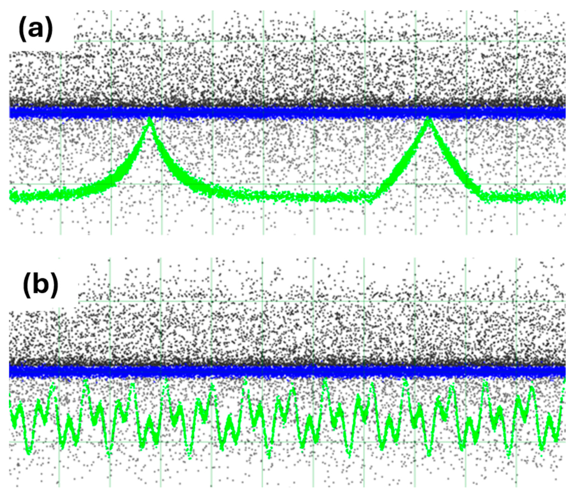
To test this hypothesis, two artificial ICESat-2 datasets comprising 100 segments each were generated with Gaussian noise added to PEs that were generated using parameters typical for real data for the following factors: track segment length, total number of PEs, ratios of PEs that constitute water surface, presence of shallow bathymetry and random noise in the air and water column. Generative parameters were established to address two basic data scenarios. In the first, Bathy PEs were arranged in a variety of slopes from completely flat to 5 degrees, and the PE heights were distributed on steeper slopes according to exponential and quadratic curves. Figure 4a shows one segment of the synthetic dataset that distributed the height of Bathy PEs using an exponential curve (left) or a quadratic curve (right) on steeper slopes. Figure 4b is an example segment of the second scenario and is the result of distributing the depth of Bathy PEs in the form of two harmonics with different spatial frequencies.

Each synthetic ICESat-2 dataset was vectorized and used to fit a LightGBM model. The two “synthetic models” were then applied separately to each of the three datasets to identify Bathy PEs. This “synthetic” classification for each dataset was then compared with the classification of Bathy PEs produced by the model that had been fitted to the manual data for the same dataset. For example, for the Key West dataset the Bathy/NotBathy prediction obtained by applying the peaks-based synthetic model to the KW dataset was compared to the Bathy/NotBathy classification produced from the model fitted for the KW dataset using the manually identified Bathy data. A high level of agreement would suggest that the synthetic data were a suitable surrogate for manually extracted data, thereby rendering the latter unnecessary.

3. Results

3.1. Algorithm Performance on Real Datasets

Table 3. Model evaluation metrics for the LightGBM model developed using the training data applied to the full datasets.

Dataset	Class	Accuracy	Precision	Recall	F1 Score	Support (% of Total)	NB + Bathy
KW	NotBathy	0.97	0.98	0.98	0.98	11,192,179 (77)	14,452,515
	Bathy		0.92	0.95	0.93	3,260,336 (23)
L&K	NotBathy	0.98	1.00	1.0	1.00	2,478,148 (83)	3,001,664
	Bathy		0.98	0.98	0.98	523,516 (17)
OSU	NotBathy	0.97	0.99	0.98	0.98	6,060,768 (90)	6,768,540
	Bathy		0.85	0.88	0.86	707,772 (10)

presents the metrics that indicate the level of agreement between the manually derived NotBathy/Bathy determination for each PE in the full datasets and the LightGBM predictions. Accuracy metrics are high for all datasets suggesting that the proposed algorithm performs well. Also notable is that the precision, recall and weighted F1 scores for NotBathy and Bathy are high and roughly equal for all datasets, suggesting that high global accuracy is not being achieved through the better accuracy of the more prevalent NotBathy class. Finally, these results largely exceed the performance of the only other ellipse-based approach of which the authors are aware [25]. That study produced F1 Scores between 0.95 and 0.99 but confined itself to three study areas in relatively clear waters and only distinguished between noise and signal PEs—i.e., it did not consider the extraction of Bathy PEs. The results in Table 3 also indicate the superior performance of the proposed method for the L&K datasets compared to the use of PointNet++ [16]; that study reported an F1 score of 0.93 for Bathy PEs compared to the 0.98 achieved by the proposed method.

A qualitative visual analysis of classification errors indicated that most false negatives (FNs) were located in areas with high local PE densities that image interpreters identified as Bathy; these FNs are likely to result from overly conservative manual processing rather than model error.

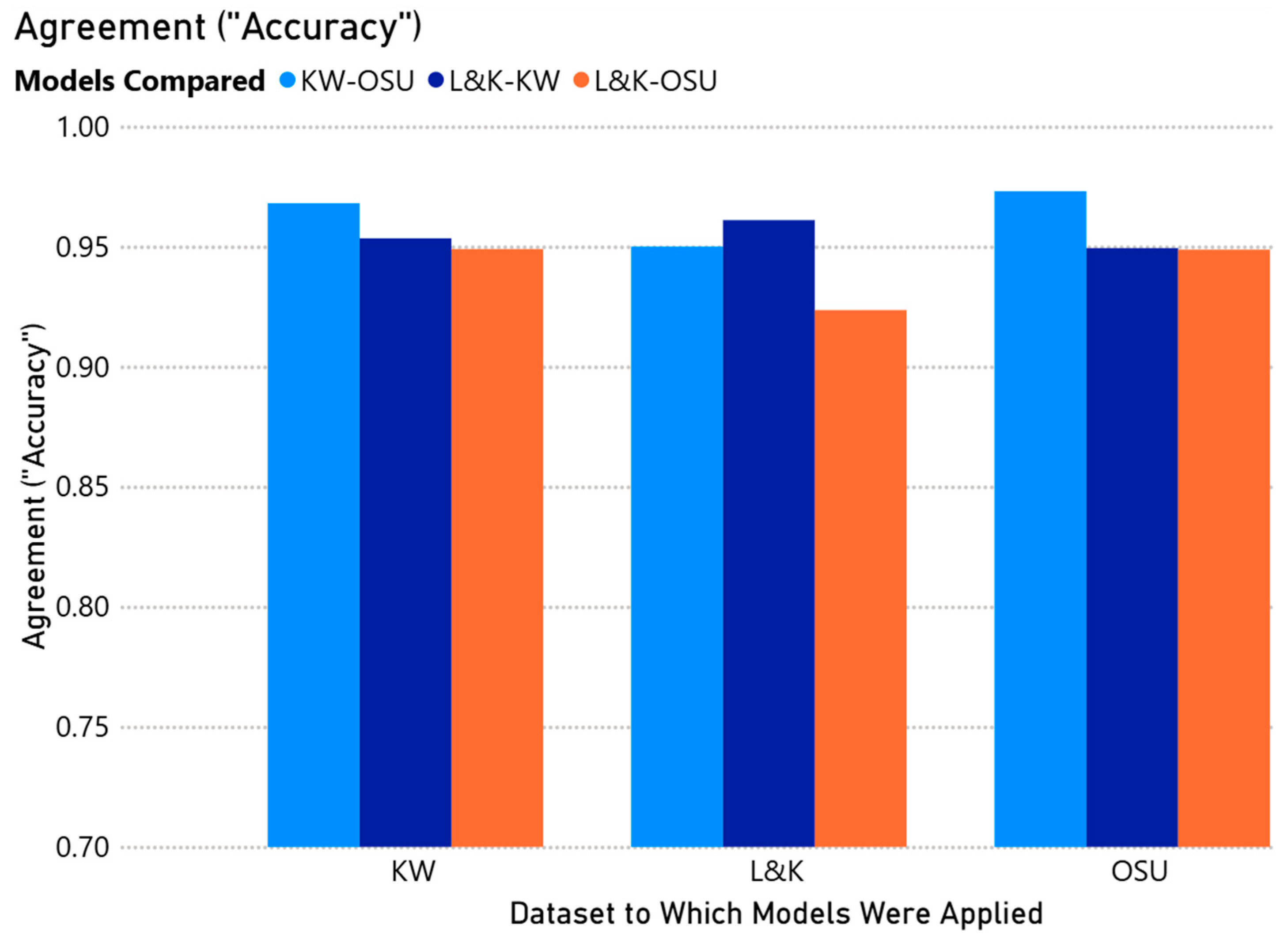
The application of each model to each of the other datasets indicates the proposed approach produces robust models (Figure 5). For example, when the two models fitted on the OSU and KW datasets were applied to the L&K dataset, the NotBathy/Bathy predictions had about 96% agreement. Agreement over all model/dataset combinations was 95% or higher except for the application of the L&K and OSU models to the L&K dataset.

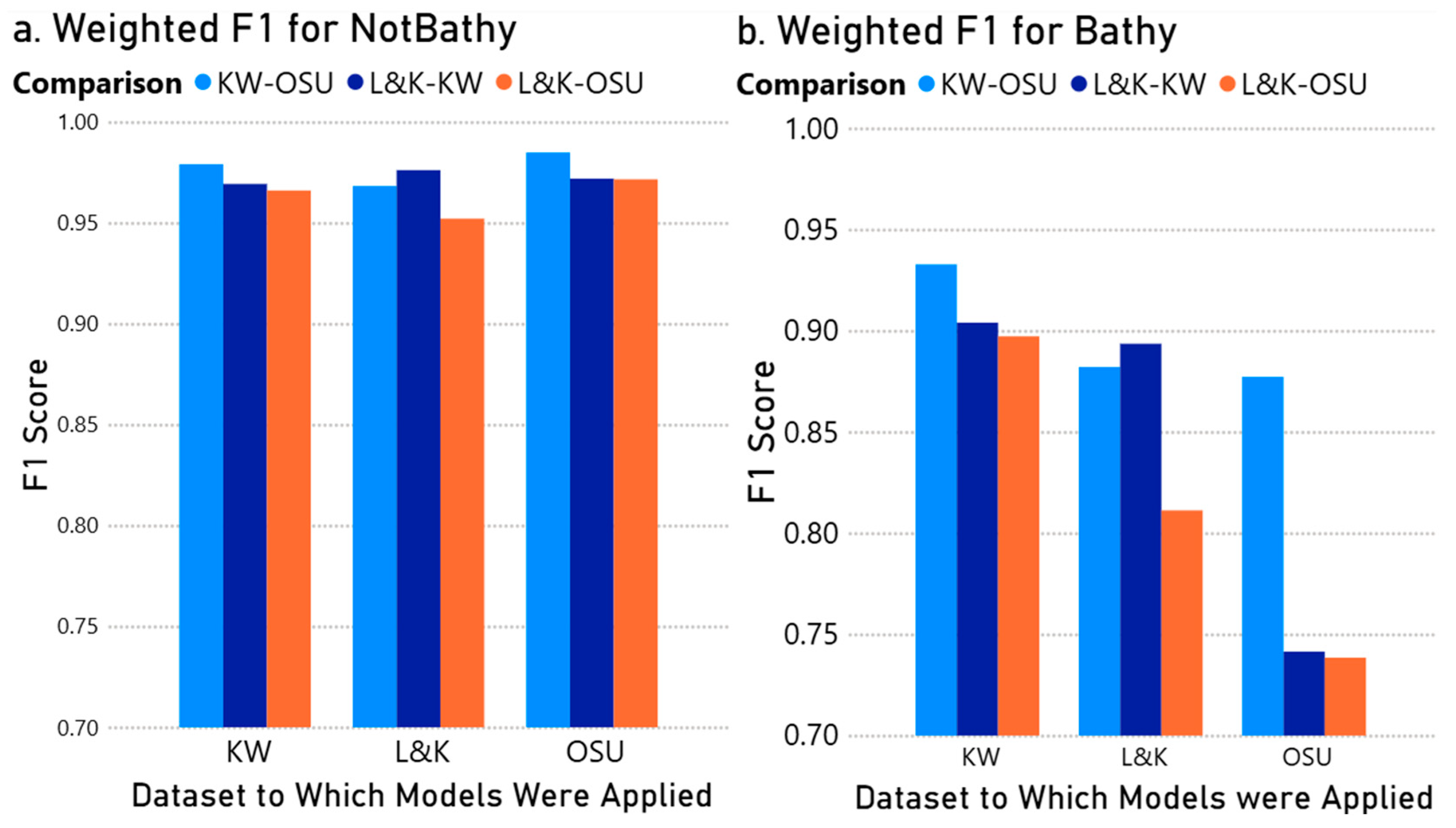
Because the agreement is impacted when individual class size (NotBathy and Bathy, in this case) is imbalanced, the F1 scores weighted by class size were also examined. Weighted F1 scores for the NotBathy class were 0.95 or above (Figure 6a). Weighted F1 scores for Bathy (Figure 6b) were lower, reflecting their lesser presence in the model fitting data. Interestingly, all models produced relatively high accuracy Bathy predictions for the KW dataset, but the Bathy predictions from the L&K- and OSU-fitted models applied to the L&K and OSU datasets showed notably less agreement. Similarly, the agreement between the predictions from the L&K-based model and both the KW- and OSU-based models produced the lowest weighted F1 scores when applied to the OSU dataset.

The LightGBM implementation employed provides an estimate of variable importance that is a normalized percentage of the number of trees in which a feature appears. Analysis of the relative importance of features (vector elements) used in model training showed that height of PEs was by far the most important feature in determining if a PE is NotBathy or Bathy. This was expected because, as noted earlier, without height in the feature vector, water surface PEs can be expected to be identified as Bathy since they have a similar structure/vectorization as Bathy PEs. In fact, without height, it is likely the water surface PEs would be the only PEs identified as Bathy since they are more dense and better structured than those representing bathymetry. The next most important variables were the number of PEs in the four sectors closest to the horizontal on both the left and right sides of the subject PE—e.g., 0 and N-2 to the right of the subject PE in Figure 3 and their “mirror sectors” on the left side. Furthermore, most important for those sectors were the ones within R1 (see Figure 3) and the least important were those within R3. This reinforces the basic premise that the relative position of PEs within a subject PE’s ellipse-defined neighborhood is highly related to the likelihood that a PE represents ocean height.

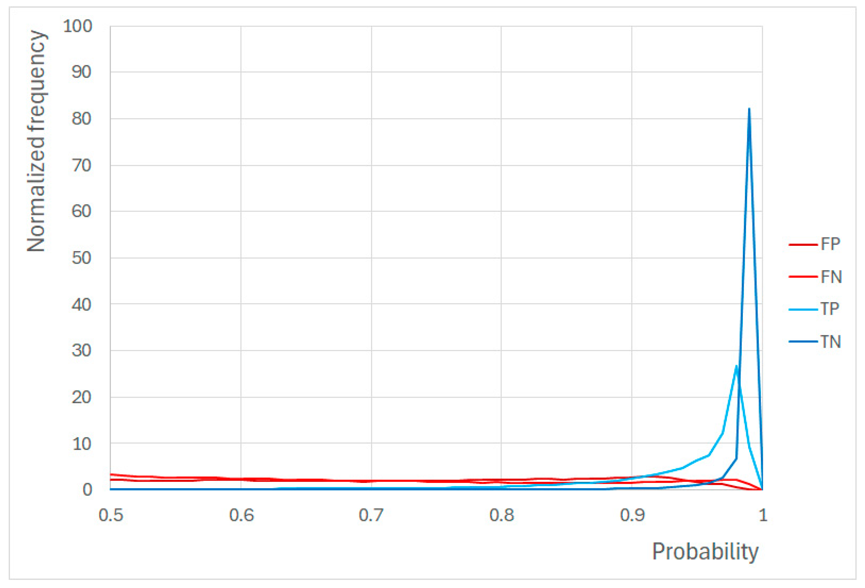
The outputs of the LightGBM model are probabilities (that sum to 1.0) that a given PE is NotBathy or Bathy. Examining these probabilities relative to classification correctness provides insight into how definitive the predictions of the proposed algorithm are. Figure 7 shows that true positives (TPs) and true negatives (TNs) form distinct peaks near high probabilities while false positives (FPs) and false negatives (FNs) are much lower in numbers and have the highest frequencies near a probability of 0.5. (At p = 0.5, a PE has an equal estimated probability of being NotBathy or Bathy). This reflects in part the high accuracy of the algorithm and model as indicated in Table 3. Moreover, it demonstrates that the certainty of FNs and FPs especially is much more variable; findings that are also reflected in the locations of FNs and FPs in Figure 7.

3.2. Evaluation of Accuracy Relative to Tuning/Hyper-Parameters

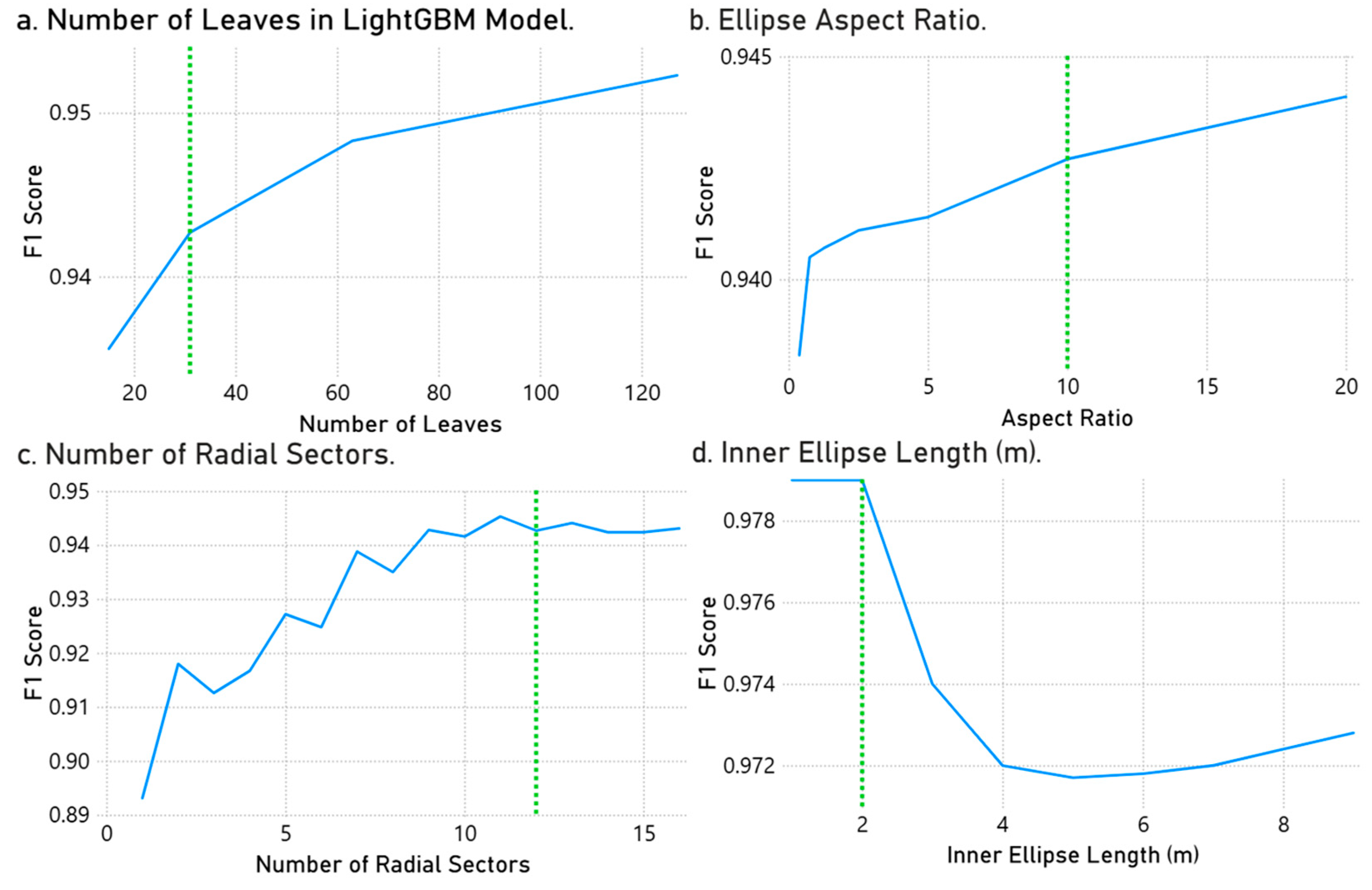
Using the KW dataset, evaluation of algorithm accuracy relative to various LightGBM models and vectorization parameters demonstrated that accuracy is not substantially changed when the parameters are varied within “reasonable” ranges. Figure 8 shows that the four factors (see also Table 2) evaluated generally indicate that, beyond a certain value of the parameter, the F1 score for Bathy PEs reaches an asymptote. Notably, the values selected for this study for these factors were neither consistently at or beyond the asymptote, nor even at the inflection point. This is because vectorization was more sensitive to the extreme values of some parameters than others. This will be addressed in the Section 4 of this paper.

The Bathy F1 score increased only slightly—from about 0.935 to 0.95—with an increase in the number of leaves over the range of values examined (Figure 8a). This indicates that model accuracy is relatively insensitive to the number of leaves used in the LightGBM model.

Figure 8b shows that the original assumption that the ellipses used in the vectorization process must have a relatively large aspect ratio—i.e., a horizontal ellipse axis longer than the vertical ellipse axis—did not prove to be crucial. That is, the F1 score did not vary widely depending on whether a circle was employed (aspect ratio = 1.0) or an elongated ellipse (aspect ratio greater than 1.0) was employed.

As expected, Figure 8c indicates that the classification accuracy did show some sensitivity to the choice of number of sectors for vectorization. However, there is clearly an asymptotic tendency when the number of sectors is beyond a value of ~10. Hence there is little reason to use a much larger number of sectors, as doing so increases computation time for vectorization. It is also noted that the use of a much smaller number of radial sectors reduces the representation of PE structure in the algorithm—e.g., using 1 (one) radial sector eliminates all description of structure. Finally, additional testing with a much larger number of radial sectors showed that the F1 score began to decrease with an increasing number of radial sectors; this was likely related to a large number of ellipse-sector “cells” having a value of 0 (zero)—i.e., such cells contained no (0) neighboring PEs.

Finally, Figure 8d shows that accuracy is related to the length of the long/horizontal axis of the inner ellipse ($R_1$). (Recall that the outer two ellipses have axis lengths $R_2=2R_1$ and $R_3=3R_1$). The best result was achieved for axis lengths of 1 and 2 m, although longer lengths decreased F1 scores by less than 1%.

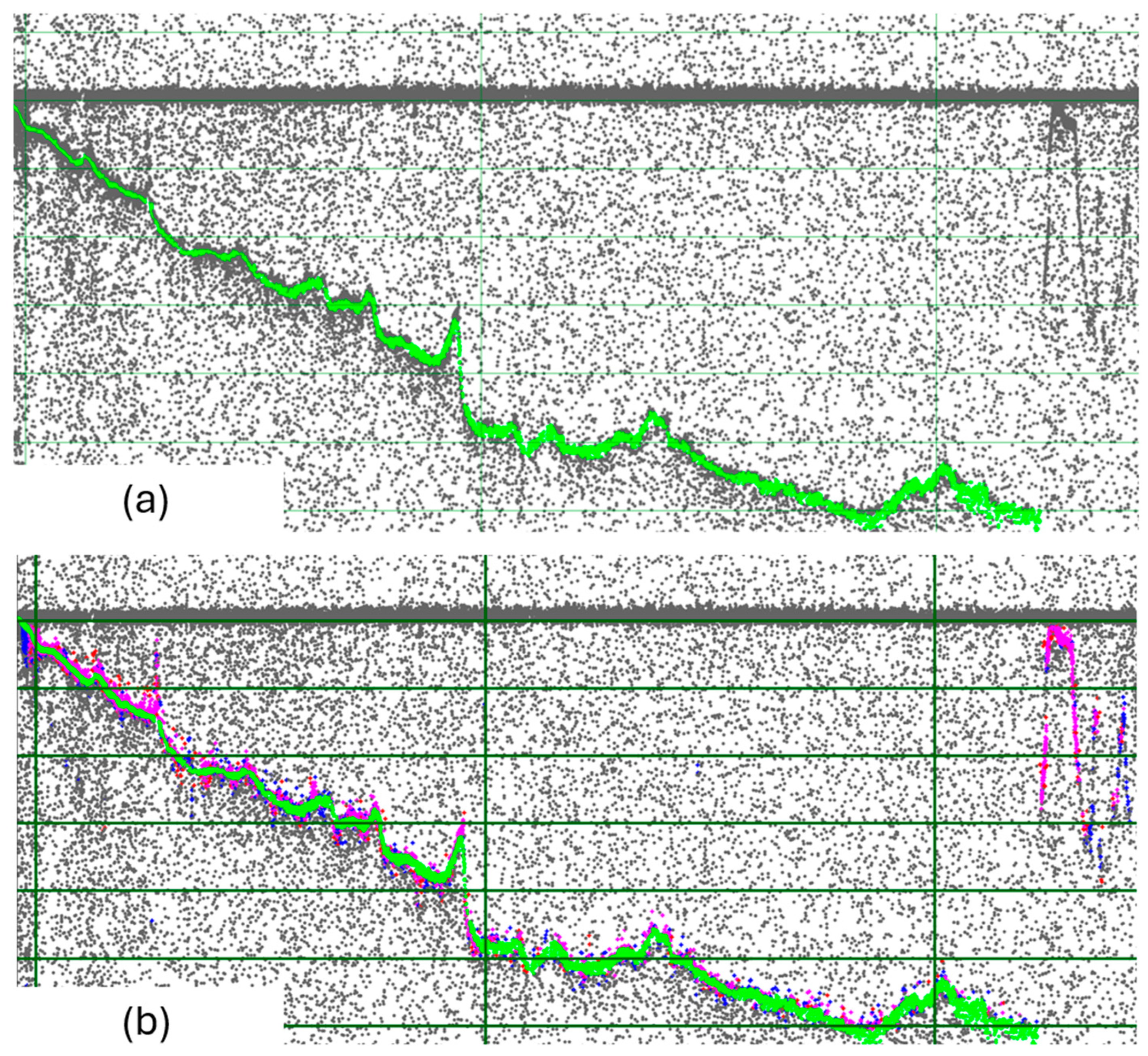
While Figure 8 shows general tendencies, visual examination of randomly selected segments showed interesting local results. Figure 9a shows the Bathy PEs manually identified by an image interpreter for a 15 km segment of an ICESat-2 track (OSU dataset [30]). The Bathy PEs were predicted using two models whose vectorizations resulted from different ellipse parameters. The purple PEs that indicate disagreement of both models with the image interpreter are more prevalent and more widely dispersed on the left side of the track; this indicates that the sea bottom in this area has an across-track slope. False positives (FPs)—PEs identified by one model (blue or red) or both models (purple) as Bathy but as NotBathy by the image interpreter—were more spatially dispersed including in areas relatively far from PEs identified as Bathy by the image interpreter. FPs are undoubtedly due to model error as they are located randomly and do not have any discernible structure; operationally these can easily be filtered out based on their local density. A prominent difference between the image interpreter and the models are the distinct structures in the upper right corner. This perhaps shows the flaw of relying on an image interpreter to develop a “ground-truth” Bathy training dataset. It is likely that the structures in the upper right corner were not labeled as Bathy by the image interpreter because the scale of display in Figure 9 suggests these structures are NotBathy. However, if the display were visually stretched to better reflect the 15 km length of this segment, the sea bottom slopes would be less dramatic, and it is likely that the image interpreter would have identified these as Bathy.

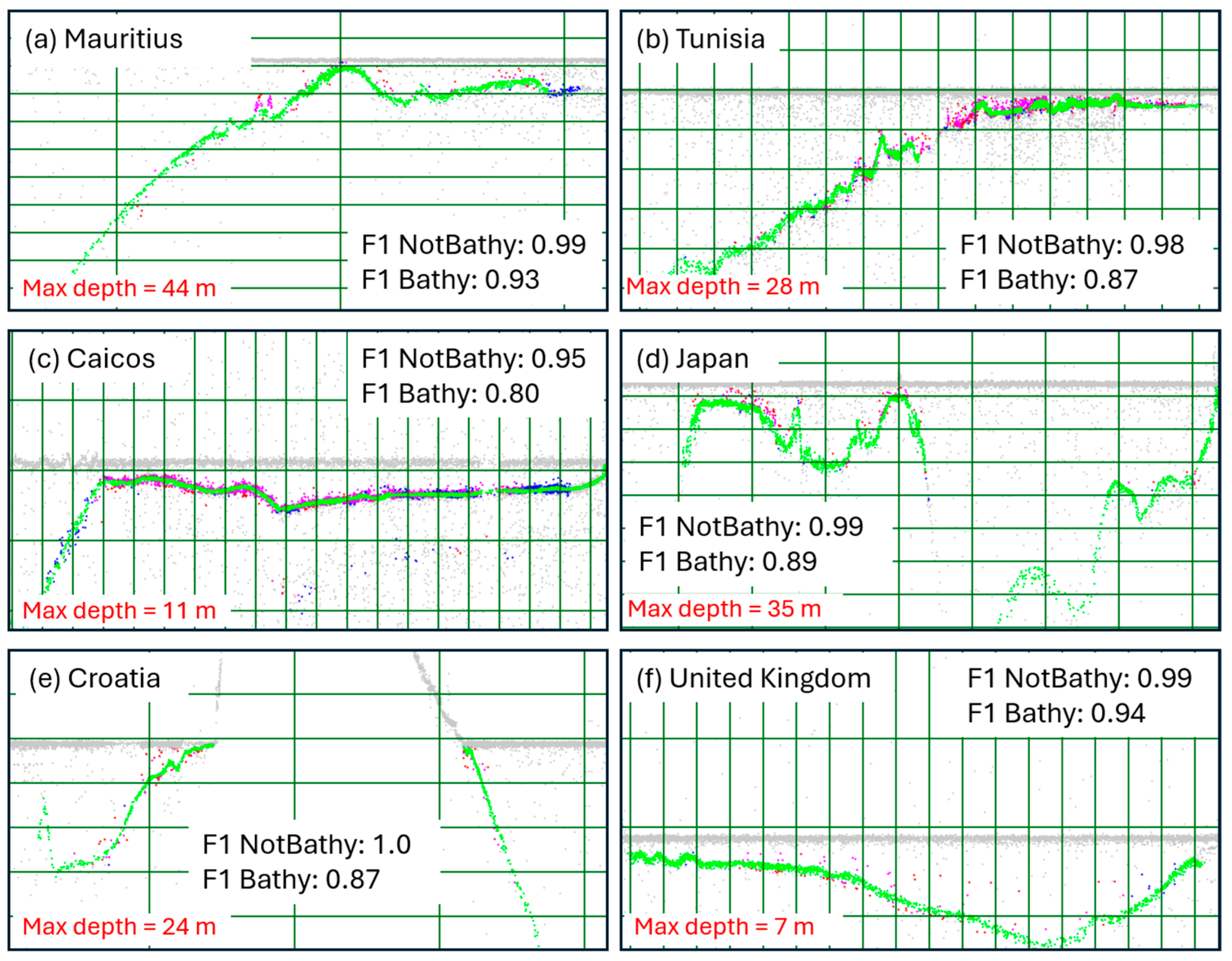
This analysis was extended by selecting six segments from the L&K dataset that were qualitatively judged to represent different morphologies; Figure 10 shows the results. There is no apparent relationship of accuracy to geomorphology in the selected segments. Neither the segment with the shallowest height (Figure 10f; UK) nor with the deepest height (Mauritius; Figure 10a) produced the highest nor the lowest Bathy F1 scores. Similarly, the segments with the most variable slopes (Figure 10d Japan and Figure 10e Croatia) produced neither the lowest nor the highest F1 Bathy scores. These results suggest that the algorithm will produce similarly high accuracy over a wide range of conditions and locations.

3.3. Using Synthetic Data for Model Training

Figure 11 shows the comparison of the Bathy PE classification for models fitted on synthetic data with the classification for a model fitted and applied to the same dataset. For example, for Key West the Bathy/NotBathy predictions from the model fitted to manually interpreted KW Bathy data were compared to the Bathy/NotBathy predictions for the KW dataset from the model fitted to the peaks-based synthetic data. Recall that strong agreement between the two classifications would suggest that synthetic training data might be a viable alternative to manually extracted data.

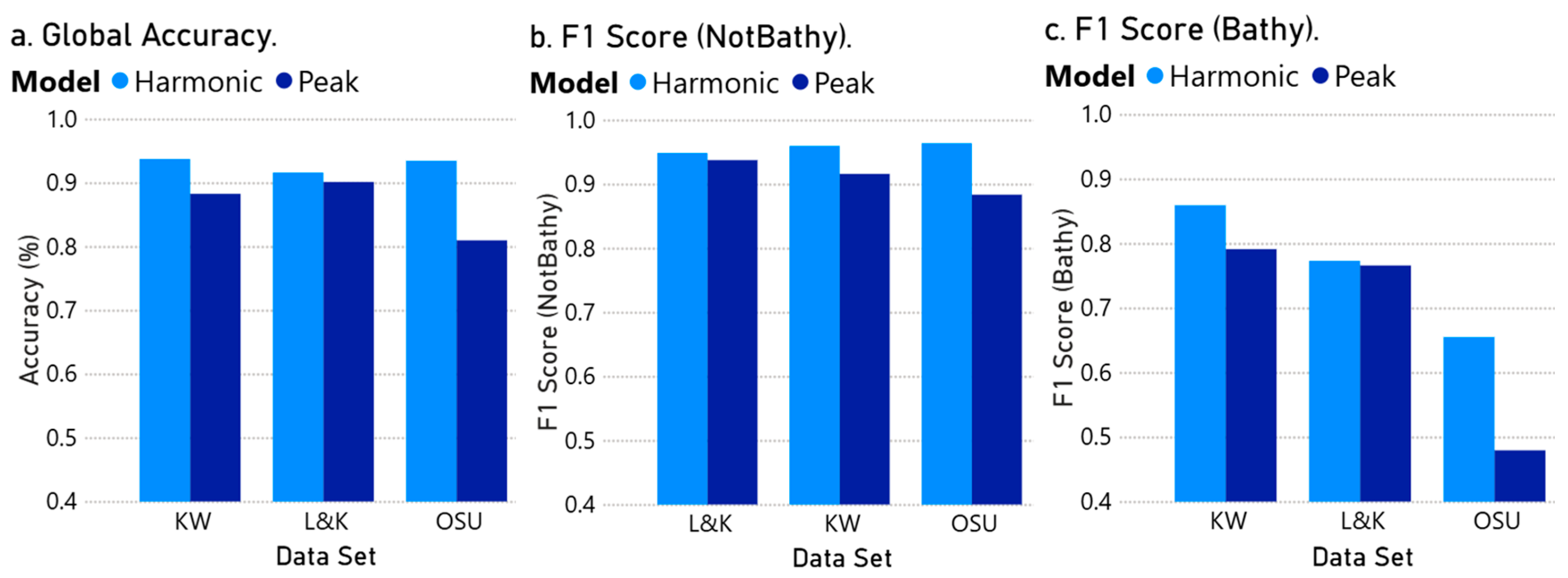
Though performance of synthetic harmonics- and peak-based models varies, in general the models based on synthetic and manually interpreted data perform comparably. “Accuracy” (“agreement” of model predictions in reality) is consistently above 0.80 with the model fitted on harmonics-based synthetic data consistently above 0.9 (Figure 11a). The NotBathy F1 scores are similarly high and roughly equal for both synthetic datasets. However, the Bathy F1 scores for the OSU dataset were relatively low, particularly for the peaks-based data. Similarly, the models fitted on the harmonics-based data outperformed the model fitted on peaks-based data. Somewhat perversely, these two results demonstrate that synthetic data could potentially be modified to reflect the characteristics of individual datasets if desired. Such modification would, of course, require examination of important data characteristics and methods for simulating them in synthetic datasets.

4. Discussion

In addition to accuracy, for operational adaptation of the proposed algorithm, processing time is also a consideration. Vectorization is the step that requires most time because it necessitates finding the PEs in each PE’s neighborhood as defined by the three ellipses. Though exact processing times are intentionally not mentioned because they vary considerably with ellipse size and PE density (as well as by computing platform), they typically varied from a few seconds to several minutes for each ICESat-2 segment when using a mid-range PC desktop platform. This relatively short processing time is undoubtedly due to the two-dimensional nature of ICESat-2 tracks that are linear rather than areal/pixel-based. Nonetheless, as is to be expected, larger ellipses and greater PE densities increase processing times with little gain in accuracy, as indicated in Figure 8.

In the development of the proposed algorithm, considerable effort was spent to identify “optimal” ellipse parameters. This was guided by practical considerations and the nature of the datasets employed. For example, it was recognized that the best combination of ellipse size and aspect ratio is related to the density of PEs in the two-dimensional along-track vs. depth space. This in turn is related to the nature of the ICESat-2 tracks available for a given area during the time period of interest. The outer ellipse must be sufficiently large to include “enough” Bathy PEs in a subject PE’s neighborhood and have “adequate” representation of the “typical” sea bottom structure (although accuracy results did not appear to be related to geomorphology—see Figure 11). Because these cannot be definitively determined for a local area of interest a priori, a sensible strategy for specifying optimal parameters for a specific area would be to classify PEs with several models trained using different parameters. This is the strategy for bathymetric extraction adopted in the recently released ICESat-2 bathymetric product ATL24 [31]. An alternative strategy would be to develop adaptive parameterization processes that could determine “optimal” parameters relative to key dataset characteristics. This would be a useful topic for future research.

The results achieved by the proposed algorithm are comparable to the best results of other algorithms reported in the review article by Jung et al. [7]. As mentioned in Section 3 (Results) a notable difference between the proposed Bathy-identifying algorithm and most others is the use of PE structure, which is generally ignored by other algorithms. One exception is the K_average nearest neighbor approach described by Meng et al. [25]. Nonetheless, accuracy metrics, particularly the F1 score—for the proposed algorithm were similar to those reported by Meng et al. A direct comparison is not possible, however, because those researchers sought to identify bathymetry or water surface PEs rather than focusing on bathymetry PEs as we have done. Though the approach of Meng et al. is consistent with the NASA ICESat-2 processing that is recorded in the attribute signal_conf_ph in the product ATL03, it did not target the identification of PEs representing the sea bottom as the proposed algorithm does. Another comparison was made with the results of [16], who applied PointNet++ to the L&K dataset also used herein. As measured by F1 scores, the proposed algorithm provided better accuracy than PointNet++.

Another potential issue is the performance of the proposed algorithm under differing environmental and water conditions. Rather than conduct comparative experiments on a necessarily limited number of datasets, global datasets were used for algorithm development and evaluation. It was considered that such datasets would provide a wider range of environmental/water conditions that would also be more representative of conditions that would be encountered in smaller area-specific datasets. That the proposed algorithm performed well on such global datasets strongly suggests a high level of robustness. This is reinforced by the results presented for the qualitative analysis that employed six tracks (see Figure 10).

One subject that was not addressed in this work—and indeed has received little attention generally—is the amount and type of data required to adequately train models as described in this paper. This was partially the motivation for the work undertaken to generate synthetic datasets that are realistic enough to train models that perform well with real ICESat-2 data. This would eliminate the need for manual identification of Bathy PEs and also enable development of locally reliable datasets. But even with synthetic datasets, the amount of data required to adequately train Bathy identification models is unknown. Moreover, given that LiDAR penetrates shallow areas best, there is a risk that shallow areas will be over-represented. This has implications for the spatial distribution of model accuracy and for the efficient extraction of Bathy PEs on which models are trained. There is a general need for research to understand the impact of the various amounts and depth characteristics of PEs used to train satellite-derived bathymetry models on model accuracy.

5. Conclusions

Table 4. Summary of results (ranges are for the three datasets employed).

Section	Subject	Figures– Tables	Results Summary Focus	Range of Results Metrics/ Conclusions
Section 3.1	Model goodness-of-fit	Table 4	Classification Accuracy	0.97–0.98
			Bathy/NotBathy F1 Scores	Bathy: 0.86–0.98 NotBathy: 0.98–1.0
	Application of “Model A” to “Dataset B”	Figure 5	Classification Accuracy	0.925–0.975
		Figure 6	Bathy/NotBathy F1 Scores	Bathy: 0.73–0.93 NotBathy: 0.95–0.98
	Uncertainty of Classification	Figure 7	Frequency distribution of p(Bathy) and p(NotBathy) relative to correctness of classification	True positives (p(Bathy)): 0.9–1.0 True negatives (p(NotBathy)): 0.97–1.0
Section 3.2	Model sensitivity to tuning/hyper- parameters	Figure 8	Change in F1 score for identification of Bathy PEs with change in parameter value	Conclusion: Sensitivity of model accuracy is low for (a) the number of leaves in a LightGBM model, (b) ellipse shape, (c) number of radial sectors dividing ellipses, (d) ellipse size.
Section 3.3	Goodness-of-fit of models fitted using synthetic data	Figure 10	Classification accuracy	0.8–0.93
			Bathy/NotBathy F1 Scores	Bathy: 0.86–0.98 NotBathy: 0.48–0.86

summarizes the results of this study.

The proposed two-step algorithm—vectorization plus model fitting—for the identification of Bathy PEs employs a quantitative description of PE structure in addition to the more conventional parameter density. The result achieves agreement with manual image interpreters of 95% or higher (global accuracy of 0.95 or better) for ICESat-2 tracks. This could potentially be especially useful in bathymetric extraction approaches that combine the results of multiple algorithms that are based on different analytical principles; the ICESat-2 bathymetric product ATL24 is one example of this.

The proposed algorithm and modeling methodology was found to be geographically robust—i.e., a model developed for one area produced similar accuracy when applied to other areas with potentially different water conditions, depths and ocean bottom characteristics. Models produced for one dataset not only produced high accuracy for the dataset on which the models were trained but also for other datasets covering more local and more global datasets.

Algorithm performance was not strongly affected by the choice of tuning parameters. The most important tuning parameter was the size of the ellipse(s) used in the model. The optimal choice depends on sea bottom morphology and density of Bathy PEs. As neither are known beforehand, the best strategy for optimization of tuning parameters may be to classify PEs with several models trained with different ellipse sizes and analyze the predicted probabilities. The time required to accomplish this should be tractable given that model accuracy was not highly sensitive to a wide range of values of tuning parameters (see Figure 8). Alternatively, the use of the machine learning technique transfer learning [32] may be appropriate.

Finally, the models trained on synthetic/generated datasets performed only slightly worse than those trained on manually annotated real data. This factor has the potential to save time and effort spent on manual annotation. Further analysis of bathymetric structures that are classified erroneously would allow for extending the synthetic dataset by adding similar structures so that an improved model can be produced that improves the existing deficiencies.

References

1. Markus, T.; Neumann, T.; Martino, A.; Abdalati, W.; Brunt, K.; Csatho, B.; Farrell, S.; Fricker, H.; Gardner, A.; Harding, D.; et al. The Ice, Cloud, and land Elevation Satellite-2 (ICESat-2): Science requirements, concept, and implementation. Remote Sens. Environ. 2017, 190, 260–273. [Google Scholar] [CrossRef]
2. Parrish, C.; Magruder, L.; Neuenschwander, A.; Forfinski-Sarkozi, N.; Alonzo, M.; Jasinski, M. Validation of ICESat-2 ATLAS bathymetry and analysis of ATLAS’s bathymetric mapping performance. Remote Sens. 2019, 11, 1634. [Google Scholar] [CrossRef]
3. Szafarczyk, A.; Tos, C. The use of green laser in LiDAR bathymetry: State of the art and recent advancements. Sensors 2023, 23, 292. [Google Scholar] [CrossRef]
4. Palm, S.; Yang, Y.; Herzfeld, U.; Hancock, D.; Hayes, A.; Selmer, P.; Hart, W.; Hlavka, D. ICESat-2 atmospheric channel description, data processing and first results. Earth Space Sci. 2021, 8, e2020EA001470. [Google Scholar] [CrossRef]
5. NSIDC (National Snow and Ice Data Center). ATL03 Data Dictionary (V07); NASA National Snow and Ice Data Center Distributed Active Archive Center: Boulder, CO, USA. Available online: https://nsidc.org/sites/default/files/documents/technical-reference/icesat2_atl03_data_dict_v007.pdf (accessed on 14 December 2025).
6. Neumann, T.; Brenner, A.; Hancock, D.; Robbins, J.; Saba, J.; Harbeck, K.; Gibbons, A.; Lee, J.; Luthcke, S.; Rebold, T. ATLAS/ICESat-2 L2A Global Geolocated Photon Data (ATL03 Version 5); NASA National Snow and Ice Data Center Distributed Active Archive Center: Boulder, CO, USA, 2021. [Google Scholar] [CrossRef]
7. Jung, J.; Parrish, C.E.; Magruder, L.A.; Herrmann, J.; Yoo, S.; Perry, J.S. ICESat-2 bathymetry Algorithms: A review of the current state-of-the-art and future outlook. ISPRS J. Photogramm. Remote Sens. 2025, 223, 413–439. [Google Scholar] [CrossRef]
8. Han, T.; Zhang, H.; Cao, W.; Le, C.; Wang, C.; Yang, X.; Ma, Y.; Li, D.; Wang, J.; Lou, X. Cost-efficient bathymetric mapping method based on massive active–passive remote sensing data. ISPRS J. Photogramm. Remote Sens. 2023, 203, 285–300. [Google Scholar] [CrossRef]
9. Xu, N.; Wang, L.; Zhang, H.-S.; Tang, S.; Mo, F.; Ma, X. Machine learning based estimation of coastal bathymetry from ICESat-2 and Sentinel-2 data. IEEE J. Sel. Top. Appl. Earth Obs. Remote Sens. 2024, 17, 1748–1755. [Google Scholar] [CrossRef]
10. Randall, H.; Christiansen, P.; Kliving, P.; Andersen, O.; Nielsen, K. Evaluation of a statistical approach for extracting shallow water bathymetry signals from ICESat-2 ATL03 photon data. Remote Sens. 2021, 13, 3548. [Google Scholar] [CrossRef]
11. Zhong, J.; Liu, X.; Shen, X.; Jiang, L. A robust algorithm for photon denoising and bathymetric estimation based on ICESat-2 data. Remote Sens. 2023, 15, 2051. [Google Scholar] [CrossRef]
12. Neuenschwander, A.; Pitts, K.; Jelley, B.; Robbins, J.; Markel, J.; Popescu, S.; Nelson, R.; Harding, D.; Pederson, K.; Sheridan, R. Ice, Cloud, and Land Elevation Satellite (ICESat-2) Project Algorithm Theoretical Basis Document (ATBD) for Land-Vegetation Along-Track Products (ATL08), Version 4; NASA National Snow and Ice Data Center Distributed Active Archive Center: Boulder, CO USA, 2021. [Google Scholar] [CrossRef]
13. Cao, B.; Wang, J.; Hu, Y.; Lv, Y.; Yang, X.; Gong, H.; Li, G.; Lu, X. ICESat-2 shallow water bathymetric mapping based on a size and direction adaptive filtering algorithm. IEEE J. Sel. Top. Appl. Earth Obs. Remote Sens. 2023, 16, 6279–6295. [Google Scholar] [CrossRef]
14. Zhang, B.; Liu, Y.; Dong, Z.; Li, J.; Chen, Y.; Tang, Q.; Huang, G.; Tao, J. An optimal denoising method for spaceborne photon-counting LiDAR based on a multiscale quadtree. Remote Sens. 2024, 16, 2475. [Google Scholar] [CrossRef]
15. Xie, C.; Chen, P.; Zhang, Z.; Pan, D. Satellite-derived bathymetry combined with Sentinel-2 and ICESat-2 datasets using machine learning. Front. Earth Sci. 2023, 11, 1111817. [Google Scholar] [CrossRef]
16. Lin, Y.; Knudby, A. Global automated extraction of bathymetric photons from ICESat-2 data based on a PointNet++ model. Int. J. Appl. Earth Obs. Geoinf. 2023, 124, 103512. [Google Scholar] [CrossRef]
17. Qin, W.; Song, Y.; Zou, Y.; Zhu, H.; Guan, H. A novel ICESat-2 signal photon extraction method based on convolutional neural network. Remote Sens. 2024, 16, 203. [Google Scholar] [CrossRef]
18. Magruder, L.; Brunt, K.; Neumann, T.; Klotz, B.; Alonzo, M. Passive ground-based optical techniques for monitoring the on-orbit ICESat-2 altimeter geolocation and footprint diameter. Earth Space Sci. 2021, 8, e2020EA00141. [Google Scholar] [CrossRef]
19. Hsu, H.-J.; Huang, C.-Y.; Jasinski, M.; Li, Y.; Gao, H.; Yamanokuchi, T.; Wang, C.-G.; Chang, T.-M.; Ren, H.; Kuo, C.-Y.; et al. A semi-empirical scheme for bathymetric mapping in shallow water by ICESat-2 and Sentinel-2: A case study in the South China Sea. ISPRS J. Photogramm. Remote Sens. 2021, 178, 1–19. [Google Scholar] [CrossRef]
20. Datta, R.; Wouters, B. Supraglacial lake bathymetry automatically derived from ICESat-2 constraining lake depth estimates from multi-source satellite imagery. Cryosphere 2021, 15, 5115–5132. [Google Scholar] [CrossRef]
21. Jia, D.; Li, Y.; He, X.; Yang, Z.; Wu, Y.; Wu, T.; Xu, N. Methods to improve the accuracy and robustness of satellite-derived bathymetry through processing of optically deep waters. Remote Sens. 2023, 15, 5406. [Google Scholar] [CrossRef]
22. Xu, Q.; Xie, H.; Sun, Y.; Liu, X.; Guo, Y.; Huang, P.; Li, B.; Tong, X. Auto-adaptive multi-level seafloor recognition and land-sea classification (AMSRLC) in reef-island zones using ICESat-2 laser altimetry. Int. Arch. Photogramm. Remote Sens. Spat. Inf. Sci. 2022, 43, 309–314. [Google Scholar] [CrossRef]
23. Zhang, G.; Xing, S.; Xu, Q.; Li, P.; Wang, D. A pre-pruning quadtree isolation method with changing threshold for ICESat-2 bathymetric photon extraction. Remote Sens. 2023, 15, 1629. [Google Scholar] [CrossRef]
24. Stephens, D.; Smith, A.; Redfern, T.; Talbot, A.; Lessnoff, A.; Dempsey, K. Using three dimensional convolutional neural networks for denoising echosounder point cloud data. Appl. Comput. Geosci. 2019, 5, 1000016. [Google Scholar] [CrossRef]
25. Meng, W.; Li, J.; Tang, Q.; Xu, W.; Dong, Z. ICESat-2 laser data denoising algorithm based on a back propagation neural network. Appl. Opt. 2022, 61, 8395–8404. [Google Scholar] [CrossRef] [PubMed]
26. Jia, K.; Ma, Y.; Zhang, J.; Wang, B.; Zhang, X.; Cui, A. A denoising methodology for detecting ICESat-2 bathymetry photons based on quasi full waveform. IEEE Trans. Geosci. Remote Sens. 2024, 62, 4207916. [Google Scholar] [CrossRef]
27. Zhang, Z.; Liu, X.; Ma, Y.; Xu, N.; Zhang, W.; Li, S. Signal photon extraction method for weak beam data of ICESat-2 using information provided by strong beam data in mountainous areas. Remote Sens. 2021, 13, 863. [Google Scholar] [CrossRef]
28. Ke, L.; Meng, Q.; Finley, T.; Wang, T.; Chen, W.; Ma, W.; Ye, Q.; Liu, T.-N. LightGBM: A highly efficient gradient boosting decision tree. In Proceedings of the 31st Conference on Neural Information Processing Systems (NIPS 2017), Long Beach, CA, USA, 4–7 December 2017; pp. 3149–3157. [Google Scholar]
29. NSIDC (National Snow and Ice Data Center). Open Altimetry Platform; NSIDC: Boulder, CO, USA. Available online: https://openaltimetry.earthdatacloud.nasa.gov/data/ (accessed on 14 December 2025).
30. Ohlwiler, E.; Ghartey, C.; McCullough, R.; Parrish, C.; Magruder, L.; Dietrich, J.; Holwill, M.; Markel, J. ICESat-2 Bathymetry Training and Testing Database [Dataset]; Oregon State University: Corvallis, OR, USA, 2023. [Google Scholar] [CrossRef]
31. Parrish, C.; Magruder, L.; Perry, J.; Holwill, M.; Swinski, J.; Kief, K. Analysis and accuracy assessment of a new global nearshore ICESat-2 bathymetric data product. Earth Space Sci. 2025, 12, e2025EA004391. [Google Scholar] [CrossRef]
32. Bozinovski, S. Reminder of the first paper on transfer learning in neural networks, 1976. Informatica 2020, 44, 291–302. [Google Scholar] [CrossRef]
Figure 1. Examples of ICESat-2 track segments (a) with bathymetric PEs and (b) without bathymetric PEs—only water surface PEs are present.
Remotesensing 18 00025 g001
Figure 2. Schematic of the algorithm modeling flow.
Remotesensing 18 00025 g002
Figure 3. Schematic of the ellipse-based structure from which each PE’s local density and structure are described using a data vector. The sectors in the vectorization table on the right are identified in the graphic on the left ( R n is the radius of the n-th ellipse shown as gray lines; 0, 1, … N − 1 are the radial sectors determined by the blue lines).
Remotesensing 18 00025 g003
Figure 4. Typical segments for two proposed synthetic datasets. Blue points are water surface; green points represent bathymetry. Gray points are noise. Height of Bathy PEs are distributed (a) according to a peaks-based exponential curve on the left side and a peaks-based quadratic curve on the right side and (b) in the form of two harmonics with different spatial frequencies.
Remotesensing 18 00025 g004
Figure 5. Agreement (“Accuracy”) between NotBathy/Bathy predictions for different models applied to a given dataset (“Accuracy” is in quotes since two model-predicted datasets are being compared rather than comparing a predicted dataset with a reference dataset of higher quality).
Remotesensing 18 00025 g005
Figure 6. Weighted F1-scores for NotBathy and Bathy between NotBathy/Bathy predictions by different models for a given dataset.
Remotesensing 18 00025 g006
Figure 7. Dependence of normalized frequency of PEs on their probability of being correctly identified as Not Bathy or Bathy.
Remotesensing 18 00025 g007
Figure 8. F1 scores for the KW model and dataset relative to various model and vectorization parameter values. The green dashed line is the selected value.
Remotesensing 18 00025 g008
Figure 9. Example 15 km ICESat-2 segment comparing image interpreter-identified Bathy PEs with Bathy PEs identified by two models fitted using different ellipse parameters. (a) Green points are manually identified Bathy PEs with which both models agree. (b) Purple PEs are NotBathy according to the image interpreter but Bathy according to both models. Red and blue PEs were identified as Bathy by the human interpreter and by only one of the models.
Remotesensing 18 00025 g009
Figure 10. Agreement of bathymetric sounding models with image interpreter. Track length is approximately 10 km. F1 scores are the average F1 scores for the two models. (1) Green points are manually identified Bathy PEs with which both models agree. (2) Purple PEs are NotBathy according to the image interpreter but Bathy according to both models. Red and blue PEs were identified as Bathy by the human interpreter and by only one of the models.
Remotesensing 18 00025 g010
Figure 11. Performance of models fitted on synthetic harmonics- and peaked-based data compared to the models fitted for a given dataset and applied to that dataset.
Remotesensing 18 00025 g011