Article

Enhancing Machine Learning-Based GPP Upscaling Error Correction: An Equidistant Sampling Method with Optimized Step Size and Intervals

1
School of Geoscience and Technology, Southwest Petroleum University, Chengdu 610500, China
2
College of Resources and Environment, Chengdu University of Information Technology, Chengdu 610200, China
3
Research Center for Digital Mountain and Remote Sensing Application, Institute of Mountain Hazards and Environment, Chinese Academy of Sciences, Chengdu 610041, China
*
Author to whom correspondence should be addressed.
Remote Sens. 2026, 18(1), 23; https://doi.org/10.3390/rs18010023
Submission received: 25 November 2025 / Revised: 19 December 2025 / Accepted: 19 December 2025 / Published: 22 December 2025

Highlights

What are the main findings?
  • Integrating geostatistical methods into the ML-based GPP upscaling correction enhances the characterization of surface heterogeneity dynamics, improves training sample representativeness, and significantly increases the accuracy of ML-based correction models.
  • When using identical interval counts, the optimal-step equidistant method consistently exceeds k-means clustering in performance metrics. This approach maintains high correction accuracy with minimized computational costs through appropriate interval selection.
What are the implications of the main findings?
  • Our method enables efficient and precise calibration of coarse-resolution GPP products, supplying robust data foundations for mountainous carbon flux quantification and ecological assessments.
  • Systematic analysis of surface heterogeneity factor contributions elucidates their mechanistic impacts on GPP estimation accuracy.

Abstract

Current machine learning-based gross primary productivity (GPP) upscaling error correction approaches exhibit two critical limitations: (1) failure to account for nonuniform density distributions of sub-pixel heterogeneity factors during upscaling and (2) dependence on subjective classification thresholds for characterizing factor variations. These shortcomings reduce accuracy and limit transferability. To address these issues, we propose an equidistant sampling method with optimized step size and intervals that precisely quantifies nonuniform density distributions and enhances correction precision. We validate our approach by applying it to correct 480 m resolution GPP simulations generated from an eco-hydrological model, with performance evaluation against 30 m resolution benchmarks using determination coefficient (R2) and root mean square error (RMSE). The proposed method demonstrates a significant improvement over previous elevation-based correction research (baseline R2 = 0.48, RMSE = 285 gCm−2yr−1), achieving a 0.27 increase in R2 and 91.22 gCm−2yr−1 reduction in RMSE. For comparative analysis, we implement k-means clustering as an alternative geostatistical method, which shows lesser improvements (ΔR2 = 0.21, ΔRMSE = −63.54 gCm−2yr−1). Crucially, when using identical statistical interval counts, our optimized-step equidistant sampling method consistently surpasses k-means clustering in performance metrics. The optimal-step equidistant sampling method, paired with appropriate interval selection, offers an efficient solution that maintains high correction accuracy while minimizing computational costs. Controlled variable experiments further revealed that the most significant factors affecting GPP upscaling error correction are land cover, altitude, slope, and TNI, trailed by LAI, whereas slope orientation, SVF, and TWI hold equal relevance.

Graphical Abstract

1. Introduction

The carbon cycle in terrestrial ecosystems is essential for sustaining biodiversity and controlling global atmospheric carbon dioxide concentrations [1,2]. Gross primary productivity, representing the total amount of organic carbon fixed through photosynthesis at the ecosystem level, is a critical flux in this cycle. Over the past decades, remote sensing (RS)-based models derived from ecological mechanisms have been the mainstream approach for simulating vegetation GPP [3,4].
Applying RS-based GPP models at regional and global scales typically involves scaling knowledge from finer to coarser resolutions, simplifying landscape complexity. For instance, the vegetation type of each pixel is represented by the predominant type within that pixel. Therefore, large-scale GPP simulations are closely dependent on the representation of surface heterogeneity, and neglecting or simplifying this heterogeneity can lead to significant biases in the final estimates [5]. Recent efforts to reduce scaling biases fall into two main categories: (1) improving the representation of surface heterogeneity by integrating sub-pixel information into model structures and parameters [6,7] and (2) developing spatial upscaling algorithms that directly correct scaling biases using surface heterogeneity information [8,9]. Several surface heterogeneity factors significantly affect vegetation photosynthesis [10,11,12] and can be categorized into endogenous and exogenous (abiotic) factors [13]. Land cover and leaf area index are widely used as endogenous heterogeneity factors due to their direct representation of vegetation types, density, and photosynthetic area. Topographic features, essential components of exogenous heterogeneity, include elevation, slope, aspect, sky view factor (SVF), topographic wetness index (TWI), and terrain niche index (TNI). Adjusting model structures and parameters to account for these heterogeneities requires iterative fine-tuning, limiting the ability to accommodate diverse surface heterogeneities. In contrast, spatial upscaling algorithms are well-suited for incorporating a wide range of surface heterogeneity information.
Introducing more sub-pixel information into spatial upscaling algorithms can further reduce GPP simulation biases [9]. Current machine learning (ML) algorithms, known for handling massive data and precisely simulating nonlinear relationships [1], are well-suited for establishing nonlinear relationships between surface heterogeneity factors and spatial scaling biases. ML algorithms can effectively utilize numerous surface heterogeneity factors [14,15], as demonstrated in large-scale ecological studies [16,17]. The representativeness of feature variables directly affects the quality of training samples and, consequently, the performance of ML models. For ML-based GPP spatial upscaling algorithms, accurately capturing surface heterogeneities improves model calibration accuracy.
The nonuniform density distributions of surface heterogeneities in mountainous environments are the major challenges for accurate estimation of GPP. The mainstream approach for capturing surface heterogeneities currently involves the classification and hierarchical statistical of sub-pixel information. For example, Chen et al. [8] classified slope into three ranges (0~20°, 21~40°, >41°), while Xie et al. [9] further subdivided slope into six types (e.g., <−30°, −30°~−15°, −15°~0°, 0°~15°, 15°~30°, >30°). These studies, which relied on simplistic or empirically determined classification thresholds to characterize surface heterogeneities, exhibited two significant limitations: (1) the subjectively defined thresholds failed to adequately represent complex nonuniform density distributions, resulting in questionable overall rationality, and such arbitrary threshold selection often yielded coincidental success, partially explaining why certain heterogeneity factors performed well in previous calibration studies while others did not; and (2) the dependence on subjective threshold settings severely constrained the generalizability of correction models across different environmental conditions. Thus, an objective classification and hierarchical method that aligns with nonuniform density distributions is crucial for enhancing model fitting and transferability. Various geostatistical methods, such as equidistant sampling, k-means clustering, mean standard deviation, quantile, and the natural breaks method [18,19] set inter-class thresholds based on actual data distribution, facilitating accurate description and capture of surface heterogeneities. As is well established, pixel variations during upscaling processes frequently deviate from normal distributions and demonstrate complex spatial heterogeneity. The mean-standard-deviation method, which heavily relies on data normality, and the quantile method, requiring balanced sample distributions, often fail to meet statistical requirements. Natural breaks face limitations in methodological research and broader application due to poor reproducibility, frequent neglect of spatial correlations, and limited interpretability. In contrast, equidistant sampling offers simplicity, interpretability, and cross-dataset comparability, while k-means clustering effectively adapts to intricate spatial patterns. Therefore, these two methods are more suitable for the development and practical implementation of methodology.
This study investigates the nonuniform density distribution characteristics of surface heterogeneity factors. By incorporating geostatistical methods, we enhance the representation of surface heterogeneity variations, improve the representativeness of ML training sample sets, and address key limitations in current ML-based GPP upscaling error correction—namely, inaccurate characterization of surface heterogeneity variations, low correction accuracy, and poor method transferability. The main work of this study is as follows: (1) to demonstrate the effectiveness of introducing geostatistical methods (equidistant sampling and k-means clustering) in improving the accuracy of ML-based GPP upscaling error correction; (2) systematically compare equidistant sampling and k-means clustering combined with comprehensive parameter optimization experiments to develop an optimized error correction scheme that achieves balanced computational accuracy and efficiency; and (3) investigate the relative importance of various vegetation and topographic heterogeneity factors in the correction process.

2. Materials and Methods

2.1. Study Area and Data Preprocessing

2.1.1. Study Area

To maintain comparability with previous studies and demonstrate the generalization capability of the optimization strategies, this work selected 16 mountainous watersheds from global flux sites according to Xie et al. [9] (Table S1). The selection criteria are as follows: (1) the average slope within a 0.5° × 0.5° area centered on the station is greater than 10°, and (2) data from the selected stations are available for at least two years.

2.1.2. Data Preprocessing

In this study, spatial resolutions of 30 m and 480 m were selected as the finer and coarser scales, respectively. The necessary data for GPP estimation and surface heterogeneity factors were prepared at these two scales. The GPP estimation data, sourced from Xie et al. [9], were derived from a hydrology-vegetation model named BTL (Boreal Ecosystem Productivity Simulator/BEPS-TerrainLab, version 2.0). BEPS is a commonly utilized framework that includes various processes associated with the carbon cycle, hydrological cycle, and energy equilibrium [20,21]. TerrainLab is designed to simulate hydrological processes influenced by topography [22]. The BTL model, which couples these two models, has demonstrated advantages in describing the control of topography on the photosynthesis of mountain vegetation. Xie et al. [9] validated the BTL model’s estimation results using daily eddy covariance (EC) GPP data from 16 research sites, finding that the model had a mean determination coefficient (R2) of 0.71 and a root mean square error (RMSE) of 2.34 gCm−2d−1.
The surface heterogeneity factors selected for this study are primarily categorized into vegetation and topographic heterogeneity factors. Vegetation heterogeneity factors include land cover and LAI. Finer Resolution Observation and Monitoring of Global Land Cover (FROM-GLC) provided the 30 m resolution land cover maps [23]. Using Landsat and MODIS reflectance data, the 30 m LAI maps were produced by the UofT LAI algorithm, the Spatial–Temporal Savitzky–Golay model (STSG), and the Enhanced Flexible Spatiotemporal Data Fusion model (IFSDAF) [24,25,26]. Topographic heterogeneity factors include elevation and derived factors such as slope, aspect, SVF, TWI, and TNI, calculated from elevation data. The 30 m resolution SRTM DEM (Shuttle Radar Topography Mission Digital Elevation Model) was accessed from the USGS website [27]. Finally, all surface heterogeneity factor grid maps were upscaled from 30 m to 480 m resolution using the following methods: (1) for categorical data, such as land cover, the maximum area aggregation method was employed; (2) for continuous numerical data, the mean aggregation method was used. This process resulted in two surface heterogeneity factor datasets at 30 m and 480 m resolutions.

2.2. Upscaling Error Correction of GPP

2.2.1. ML-Based GPP Upscaling Error Correction

The ML-based GPP upscaling error correction framework is designed to address errors caused by oversimplified vegetation and topographic heterogeneity in the upscaling process. Its fundamental principle states that higher-resolution input data can more accurately capture surface heterogeneity characteristics, thereby producing simulation results closer to actual values.
The framework implements a three-step processing workflow:
(1)
Using aggregated fine-resolution GPP data at coarse resolution (referred to as distributed GPP) as reference truth;
(2)
Establishing nonlinear relationships between surface heterogeneity features and upscaling errors through machine learning algorithms;
(3)
Deriving more accurate corrected results via “original coarse-resolution GPP (referred to as lumped GPP) minus predicted error” calculation.
This methodology significantly enhances the accuracy of upscaled products by quantifying heterogeneity information loss induced by resolution change. This study treats the 30 m resolution GPP as distributed GPP (GPPd), while the 480 m resolution GPP is referred to as lumped GPP (GPPl). The relationship between GPPd and GPPl is constructed as follows:
G P P d = G P P l + Δ G P P
where ΔGPP represents the impact of surface heterogeneities included in GPPl. It can be described as a function of two indicators:
Δ G P P = f S S I v e g e   , S S I t o p o
where SSIvege and SSItopo are scale indices related to vegetation heterogeneity and surface topographic heterogeneity, respectively. They can be described as
S S I v e g e = f ( L C ,   L A I )
S S I t o p o = f ( E l e ,   S l o p e ,   A s p e c t ,   S V F , T W I ,   T N I )
where Ele is elevation, SVF stands for sky view factor, TWI is the topographic wetness index, and TNI is the terrain niche index, which can be found in the corresponding literature [28,29].
Combining Equations (2)–(4), ΔGPP can be described as a function of surface heterogeneity factors:
Δ G P P = f ( L C ,   L A I ,   E l e ,   S l o p e ,   A s p e c t ,   S V F ,   T W I ,   T N I )
During the aggregation process, a coarse pixel is defined as the average of its sub-pixels or the type with the largest area. The loss of information about surface heterogeneity factors during the upscaling process is a major source of error in the lumped GPP. Therefore, a nonlinear relationship between ΔGPP and the variations in surface heterogeneity factors can be established as follows:
Δ G P P = R F ( F L C , V F L A I , V F E l e , V F S l p o e , V F A s p e c t , V F S V F , V F T W I , V F T N I )
where RF refers to the random forest algorithm, which has been widely used for simulating nonlinear relationships and has achieved good results [30,31]. Two additional motivations for selecting the RF algorithm include (1) its capacity to generate variable importance rankings, facilitating analysis of the relative contributions of surface heterogeneity factors; and (2) minimal parameter configuration requirements, with hyperparameter optimization implementable through R’s well-established caret package. As formalized in Equation (6), ΔGPP serves as the predictor variable, while changes in seven surface heterogeneity factors comprise the training dataset for model training and subsequent prediction. FLC is a set of percentages of each land cover type in a lumped pixel, as follows:
F L C = F L C i
where F L C i is the area fraction of land cover type i. If there is no type i in the lumped pixel, then F L C i is set to zero. VFLAI, VFEle, VFSlope, VFAspect, VFSVF, VFTWI, and VFTNI are the area percentages of changed LAI, elevation, slope, aspect, SVF, TWI, and TNI within the lumped pixel, respectively. For example, VFLAI can be represented as
V F L A I = F L A I d L A I 4 , F L A I 4 < d L A I 2 , F L A I 2 < d L A I 0 , F L A I 0 < d L A I 2 , F L A I 2 < d L A I 4 , F L A I d L A I > 4
where dLAI is the difference between the sub-pixel value and the lumped pixel value. For example, F L A I d L A I > 4 represents the area percentage where the difference between the sub-pixel value and the lumped pixel value is greater than 4.

2.2.2. Introducing Geostatistical Methods to Capture Surface Heterogeneity

From Equations (6) and (8), it can be observed that accurately capturing sub-pixel surface heterogeneities is critical to enhancing the model’s calibration capability. An analysis of the distribution characteristics of sub-pixel surface heterogeneity variation values reveals that most sub-pixels exhibit minimal or no change. As the intensity of variation increases, the number of changing sub-pixels decreases, demonstrating nonuniform distributions. Previous research neglected this nonuniform distribution characteristic, relying solely on subjectively determined thresholds or intervals to characterize surface heterogeneity variations. This approach fails to capture dominant sub-pixel change features or results in dominant features being masked by secondary features. Consequently, the representativeness of training samples is compromised, ultimately diminishing the calibration accuracy of ML models.
Considering the density curves of sub-pixel surface heterogeneities, which peak at 0 and are approximately uniformly distributed in both positive and negative directions, this study adopted the equidistant sampling method for classification. The primary approach was to divide the intervals equally in the positive and negative directions from zero as the center (e.g., <−10, −10~0, 0~10, >10), ensuring that the main surface heterogeneities were captured as much as possible. The k-means clustering method is a widely used unsupervised classification method, which was compared with the equidistant sampling method in this study [32,33]. This approach categorizes the density distributions of surface heterogeneities into k categories and divides them into k intervals based on the demarcation points between categories. This study optimized the error correction method using these two objective classifications and hierarchical strategies. The overall methodological process is shown in Figure 1 The expected results of this study are as follows: (1) fully considering the nonuniform density distributions of surface heterogeneities, optimizing data organization, and improving the training and prediction accuracy of the RF model; and (2) avoiding manual intervention to make the process more objective, facilitating automated operation and method transfer.

2.3. Experimental Design

2.3.1. Parameter Setting Experiment

The step and number of intervals are two essential parameters for classification and hierarchical using the equidistant sampling method. This study employs a trial-and-error approach based on controlling variables to test the impact of steps and the number of intervals on calibration accuracy, aiming to identify the optimal step and number of intervals. To this end, the following two experiments are designed for cases where a single surface heterogeneity factor is involved in spatial bias correction (Table 1).
Experiment I: Referring to previous studies, the number of equal intervals is set to 6, and the step is incremented from 0. This experiment will compare and analyze the impact of different steps on calibration accuracy and identify the optimal step that maximizes calibration accuracy.
Experiment II: The optimal step identified in Experiment I is used for interval division. For testing the effect of increasing the number of intervals on calibration accuracy, 6, 8, and 10 intervals were added, respectively. It is important to note that reducing the total number of intervals to 2 or 4 would not be sufficient.
The number of categories is a crucial parameter for the k-means clustering method, directly affecting the number of intervals. This study investigates (1) the calibration capability of the equidistant sampling method and the k-means clustering method when the same number of intervals is set and (2) the calibration performance of the equidistant sampling method and the k-means clustering method when the number of intervals is continuously increased. To achieve this, the following two experiments are set up.
Experiment III: The number of categories is set to 6, 8, and 10, corresponding to divisions into 6, 8, and 10 intervals, respectively. This experiment tests the effect of increasing the number of intervals on calibration accuracy and compares the results with the equidistant sampling method in Experiment II.
Experiment IV: The number of categories and, thereby, the number of intervals is continuously increased (from 6 to 36) to test the performance of both the equidistant sampling method (using the optimal step size obtained in Experiment I) and the k-means clustering method when a sufficient or an excessive number of intervals is set.

2.3.2. Factor Combination Experiment

Based on the comparative experiments of the two geostatistical methods mentioned above, the method demonstrating higher precision and lower computational cost was selected for upscaling error correction involving all surface heterogeneity factors. Multiple control tests were designed to analyze the impact of individual or combinations of heterogeneity factors on correction effects, as outlined in Table 2. By comparing the precision with and without the involvement of specific factors in the correction process, the study objective was to identify the best correction scheme by ranking surface heterogeneity factors.

2.3.3. Evaluation Index

R2, RMSE, and MAE, as commonly used evaluation indicators in spatial scale research, are employed for the comprehensive assessment of correction accuracy in this study. The calculation formulas are as follows:
R 2 = 1 i = 1 n y i y i ^ 2 i = 1 n y i y i ¯ 2
R M S E = 1 n i = 1 n y i y i ^ 2
M A E = 1 n i = 1 n ( y i y i ^ )
where n is the total number of pixels, yi and y i ^ represent the GPPd and the corrected GPPl of pixel i at a resolution of 480 m, respectively, and y i is the average GPPd of all pixels.

3. Results

3.1. Correction Effect Using the Equidistant Sampling Method

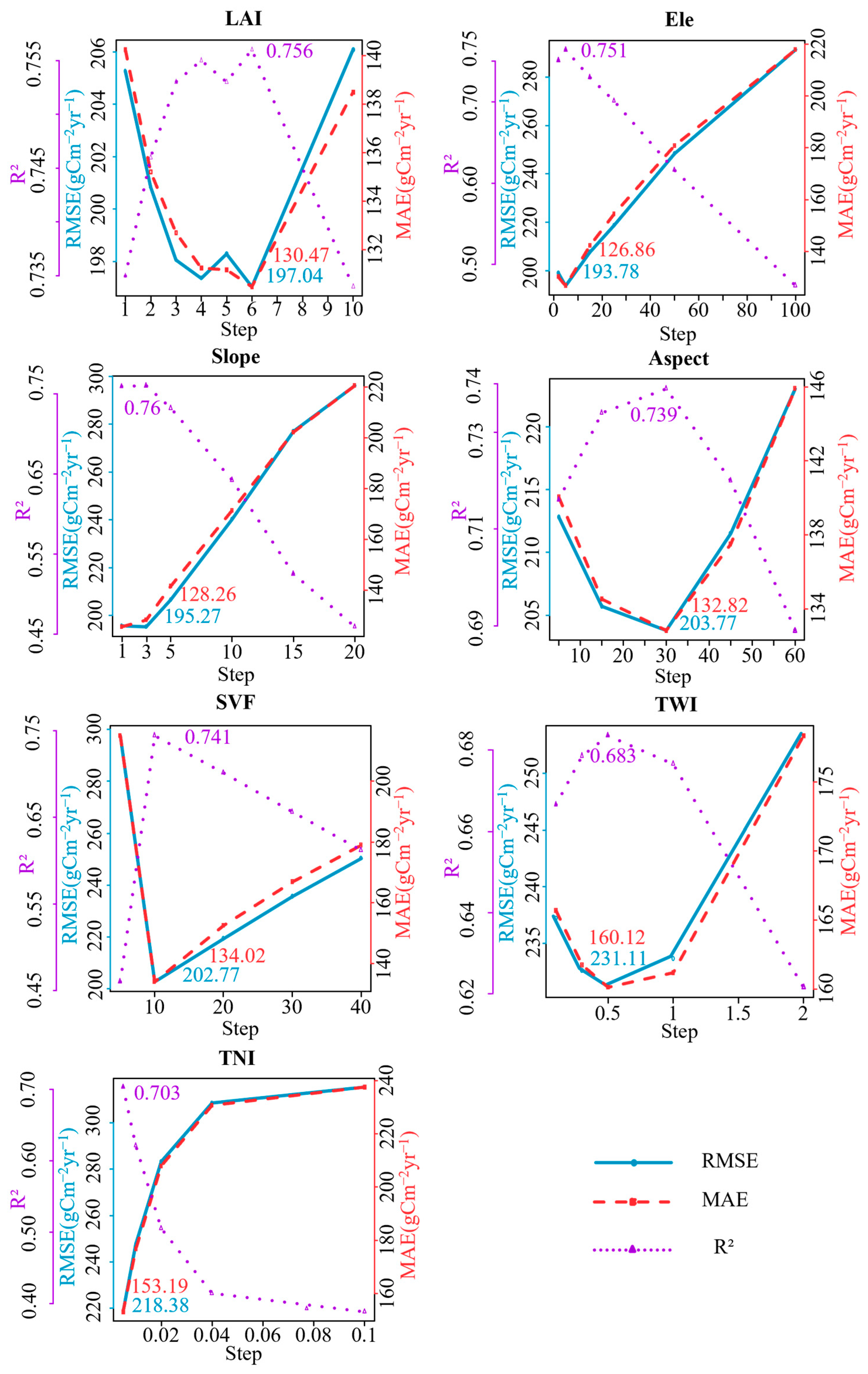
Experiment I divided the range of variation values for various surface heterogeneity factors into six fixed intervals with different steps. The correction effect of individual surface heterogeneity factors on GPP was tested under varying steps, and the results are presented in Figure 2. Each surface heterogeneity factor exhibited an optimal step that maximized the correction accuracy of GPP. For example, elevation (Ele) achieved the highest correction accuracy at a step of 5, with an R2 value of 0.751 and RMSE and MAE values of 193.78 gCm−2yr−1 and 126.86 gCm−2yr−1, respectively. Compared to previous studies, Ele’s correction accuracy improved by 0.27 in R2 and decreased RMSE by 91.22 gCm−2yr−1. Significant improvements were observed for other factors at their optimal steps, as detailed in Table 3. Moreover, the impact of step size on correction accuracy exhibited two distinct patterns as it increased. One pattern showed an initial gradual increase in accuracy, reaching an optimum, followed by a decline, observed with LAI, aspect, and SVF. The other pattern achieved relatively high correction accuracy at smaller steps, progressively decreasing as the step increased, as seen with Ele, slope, TWI, and TNI.
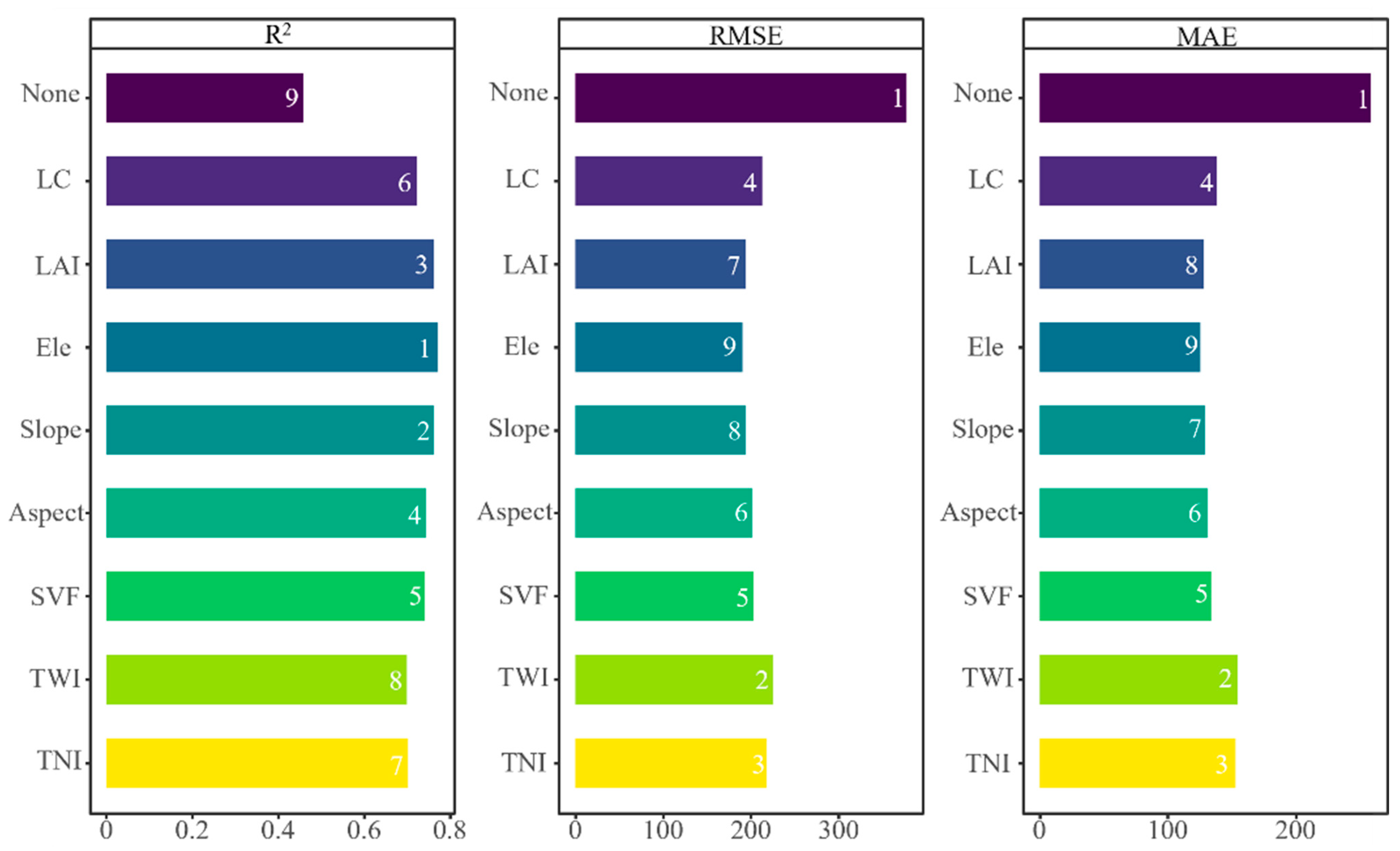
In Experiment II, the optimal steps for each surface heterogeneity factor identified in Experiment I were utilized for interval division, and the number of intervals was further increased from 6 to 8 and 10. The variations in correction accuracy for each factor with the increased number of intervals were compared, and the results are presented in Table S2. Generally, each factor exhibited an optimal number of intervals that maximized correction accuracy, although the increase in accuracy with more intervals was marginal. For example, when using LAI alone for correction, increasing the number of intervals to 8 and 10 resulted in only slight improvements in R2 by 0.005 and 0.006, respectively, along with reductions in RMSE by 1.81 gCm−2yr−1 and 2.29 gCm−2yr−1 and in MAE by 1.74 gCm−2yr−1 and 2.03 gCm−2yr−1, respectively. As the number of intervals increased, factors such as LAI, Ele, and TWI showed improved correction accuracy, while factors like slope and aspect initially increased and then decreased accuracy. Factors like SVF and TNI exhibited decreased accuracy with an increase in intervals. As depicted in Figure 3, when each factor selected the optimal step and the optimal number of intervals for equidistant capture the surface heterogeneities, using Ele alone for correction yielded the highest accuracy, with an R2 of 0.771 and RMSE and MAE values of 190.67 gCm−2yr−1 and 125.47 gCm−2yr−1, respectively. The accuracy of correction using the remaining factors alone, ranked from highest to lowest, was slope, LAI, aspect, SVF, land cover (LC), TNI, and TWI.

3.2. Correction Effect Using the K-Means Clustering Method

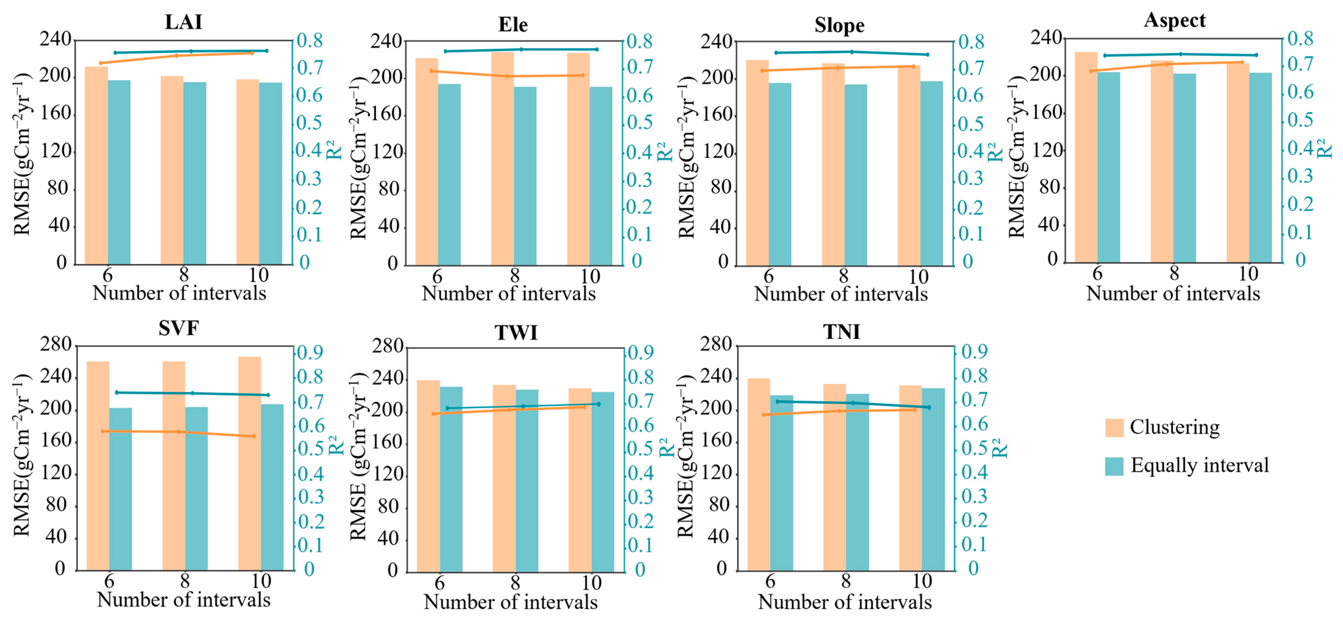
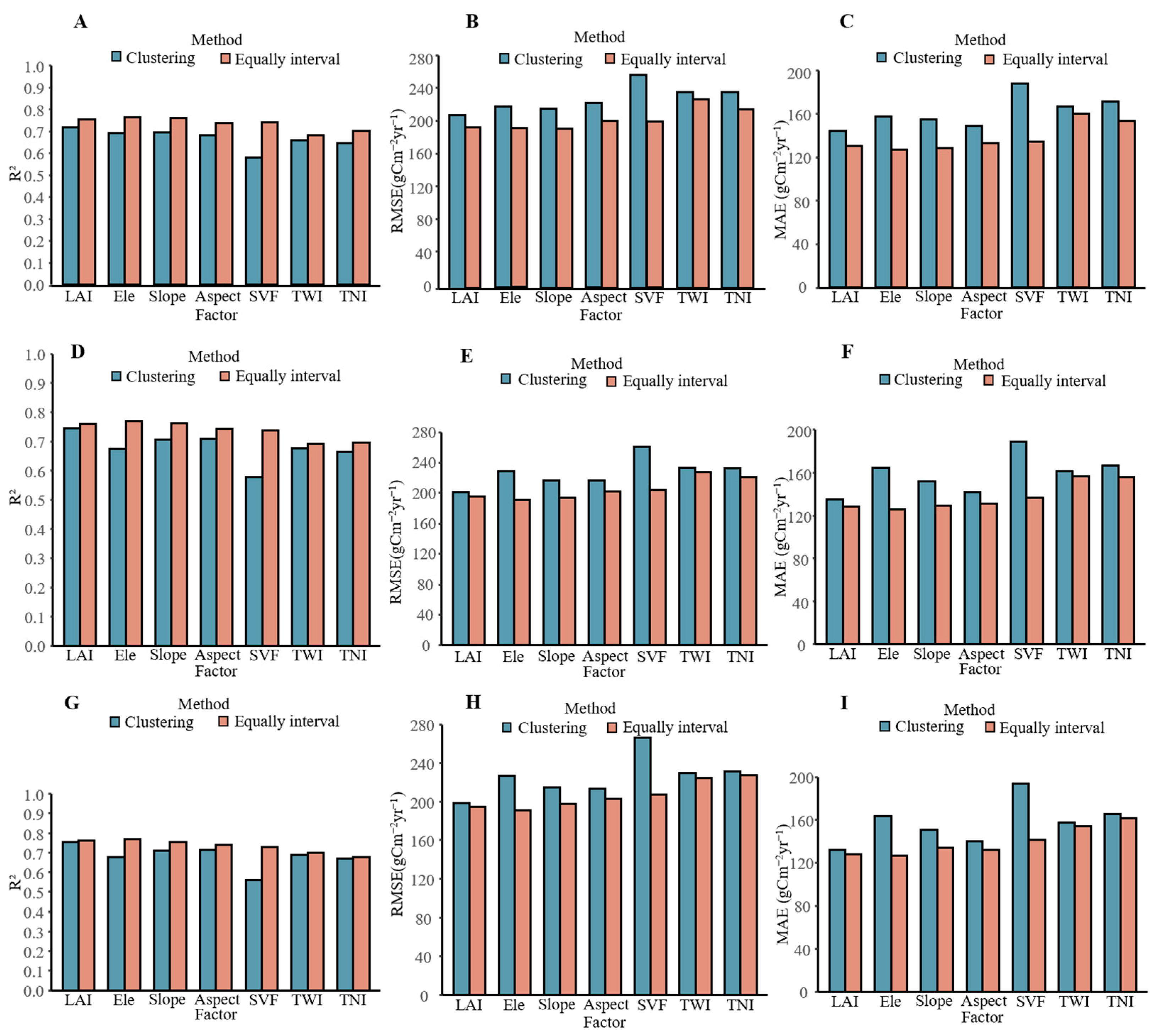
Experiment III entailed setting the number of clustering categories to 6, 8, and 10, thereby dividing the density distributions of surface heterogeneity factors into corresponding intervals. The analysis focused on the variations in correction accuracy for each factor with the increased number of intervals, comparing the correction effects of the optimal-step equidistant sampling method and the k-means clustering method with the same number of intervals, as detailed in Table S3. Increasing the number of intervals consistently enhanced correction accuracy. For instance, when using LAI alone for correction, expanding the number of intervals to 8 and 10 led to R2 improvements of 0.026 and 0.035, respectively, and reductions in RMSE by 10.28 gCm−2yr−1 and 13.86 gCm−2yr−1 and in MAE by 9.11 gCm−2yr−1 and 11.63 gCm−2yr−1, respectively. As depicted in Figure 4, the k-means clustering method demonstrated a more pronounced improvement in correction accuracy with an increase in the number of intervals compared to the optimal-step equidistant sampling method. With more intervals, factors such as LAI, slope, aspect, TWI, and TNI showed enhanced correction accuracy, while factors like Ele and SVF exhibited decreased accuracy. Figure 5 illustrated that, when using the same number of intervals, the optimal-step equidistant sampling method consistently outperformed the k-means clustering method in correction accuracy. For instance, when using slope alone for correction with 6, 8, and 10 intervals, the optimal-step equidistant sampling method achieved an average R2 that was 0.054 higher than that of the k-means clustering method, with lower RMSE and MAE values by 21.44 gCm−2yr−1 and 22.05 gCm−2yr−1, respectively.
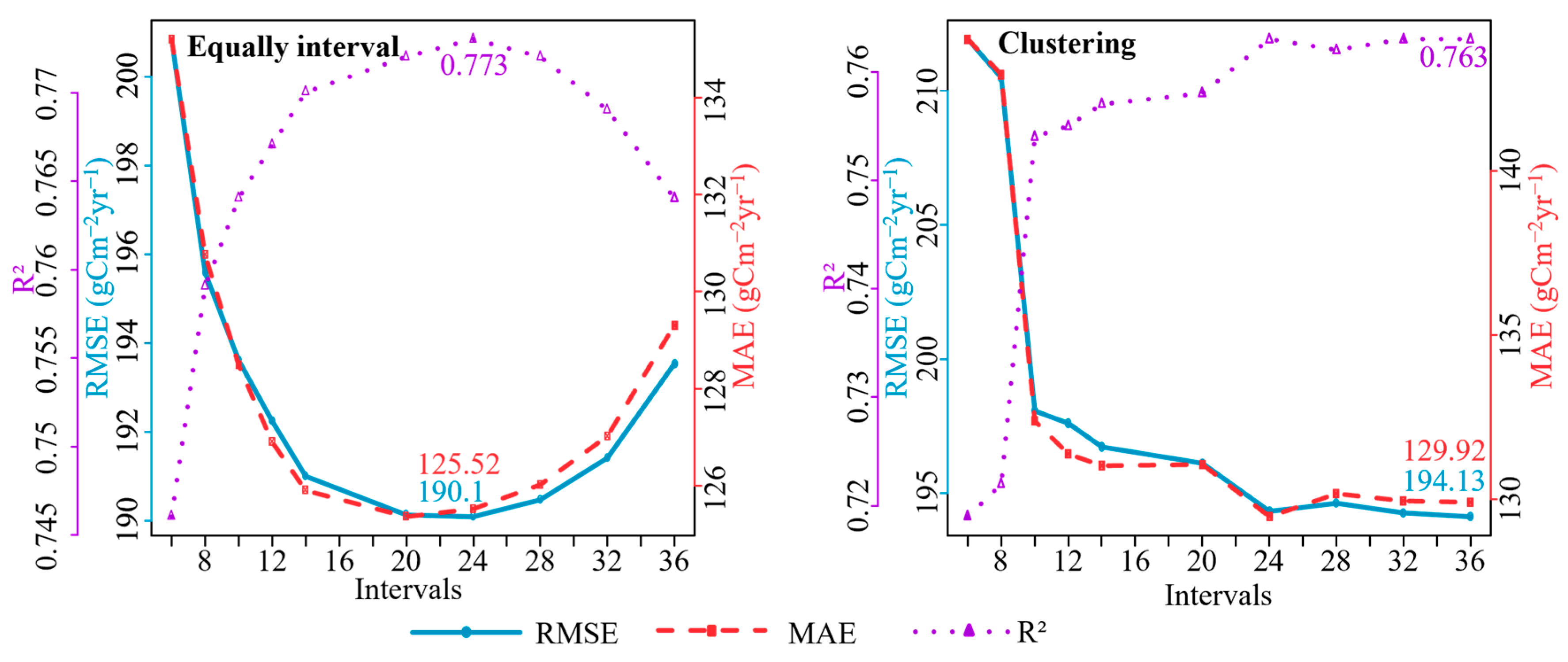
Experiment IV focused on LAI as the subject and aimed to incrementally increase the number of intervals for both the optimal-step equidistant sampling method and the k-means clustering method, analyzing their respective variations in correction accuracy, detailed in Table S4. As the number of intervals increased from 6 to 36, both methods demonstrated improved accuracy. Notably, with the same number of intervals set, the optimal-step equidistant sampling method consistently outperformed the k-means clustering method in correction accuracy. As depicted in Figure 6, the correction accuracy of the optimal-step equidistant sampling method initially increased and then decreased with the number of intervals, achieving its peak accuracy (R2 = 0.773) at 24 intervals. In contrast, the correction accuracy of the k-means clustering method increased with the number of intervals. Then, it stabilized, reaching its highest accuracy (R2 = 0.763) at 24 intervals and maintaining relative stability afterward. Thus, by increasing the number of intervals, both the optimal-step equidistant sampling method and the k-means clustering method could attain comparable levels of accuracy, highlighting the effectiveness of methodological adjustments in enhancing correction precision for spatial heterogeneity factors like LAI.

3.3. Correction Effect Using the Superior Method

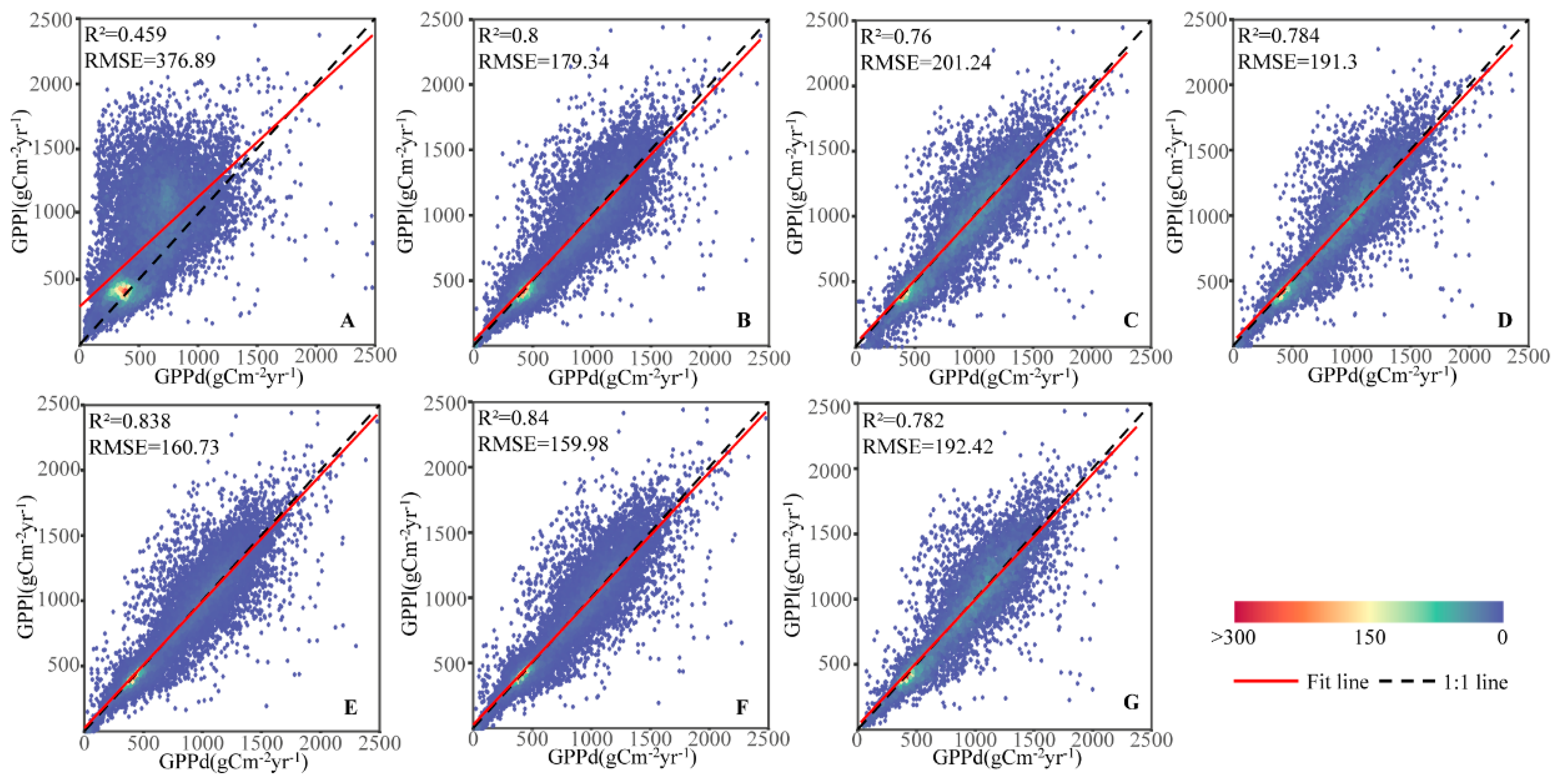
Based on the results from the previous experiments, the optimal-step equidistant sampling method consistently outperformed the k-means clustering method when the same number of intervals was set. The k-means clustering method required more intervals to achieve accuracy comparable to the optimal-step equidistant sampling method. Considering both correction effectiveness and computational efficiency, the optimal-step equidistant sampling method was selected for combining surface heterogeneity factors in further experiments. The experiments utilized the optimal step for each factor, with two schemes for setting the number of intervals: (1) using only six intervals and (2) selecting the optimal number from six, eight, and ten intervals. Each combination experiment was thus divided into two sub-experiments to analyze and determine the optimal correction scheme. The results are summarized in Table S5. The control group, representing uncorrected GPPl, had an R2 of 0.459, RMSE of 376.89 gCm−2yr−1, and MAE of 258.66 gCm−2yr−1 compared to GPPd. Across the tests, the combination corrections significantly enhanced accuracy, with the highest improvement seen in Test 5, achieving an R2 increase of 0.301 and reductions in RMSE and MAE by 175.65 gCm−2yr−1 and 127.76 gCm−2yr−1, respectively. Tests involving TWI generally showed lower accuracy compared to those without it. For instance, Test 6, which included TWI alongside other factors, exhibited decreased R2 from 0.838 to 0.782 and increased RMSE and MAE.
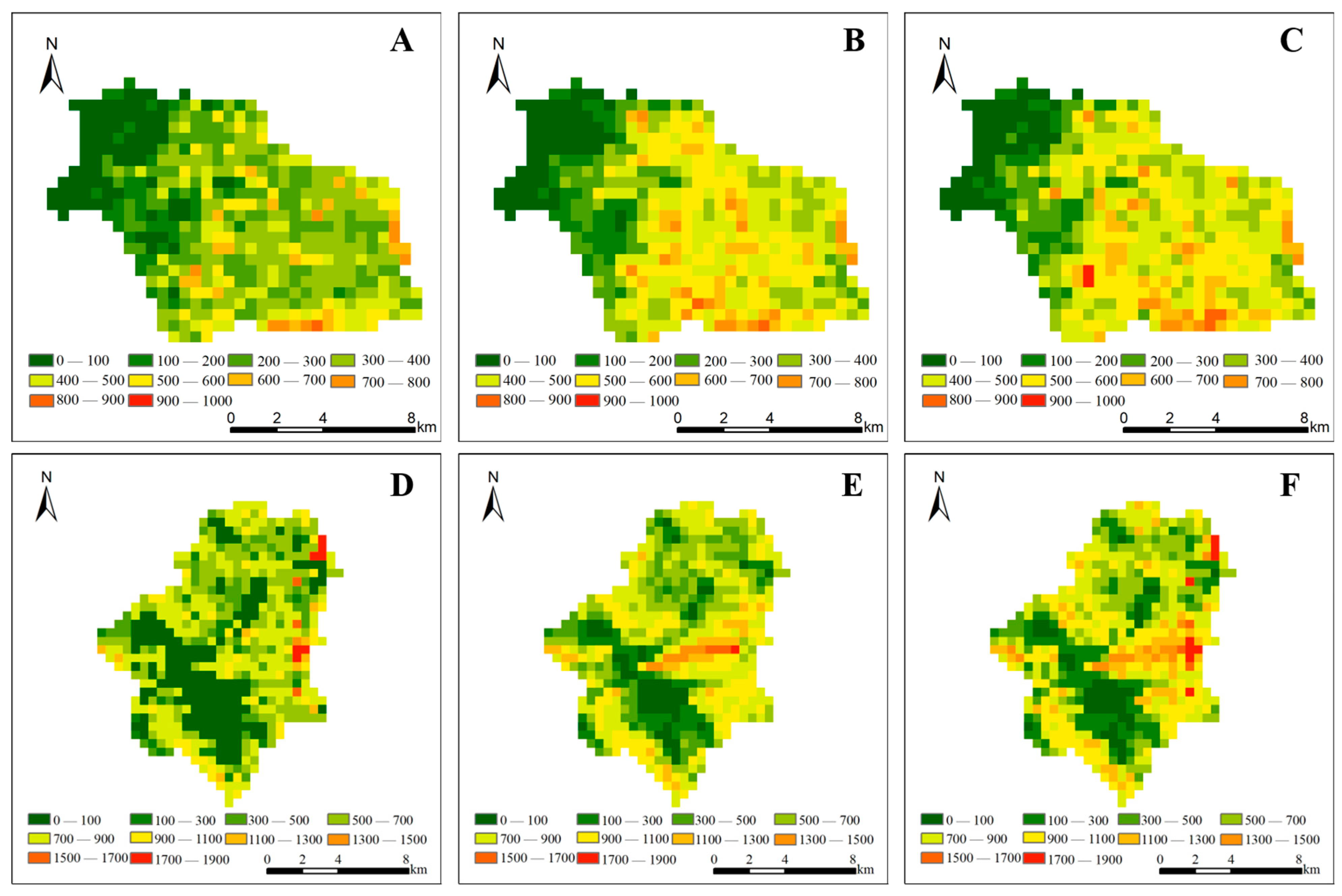
Figure 7 illustrates that Test 5, incorporating LC, LAI, Ele, slope, aspect, SVF, and TNI, achieved the highest accuracy among the experiments. The comparison between sub-experiments using six intervals and the optimal number of intervals showed comparable correction effects, with minimal differences in RMSE and MAE. However, selecting the optimal number of intervals incurred higher computational costs compared to using only six intervals. In conclusion, adopting LC, LAI, Ele, slope, aspect, SVF, and TNI factors with optimal steps and six intervals for equidistant variation capture represents the optimal scheme balancing high accuracy and lower computational burden. As depicted in Figure 8, this approach effectively enhances correction accuracy for GPPl while maintaining computational efficiency. Meanwhile, as shown in Figure 9, applying this correction scheme to a single site also showed a detailed improvement in visual effects.

4. Discussion

4.1. Improvement of Correction Accuracy by Considering Nonuniform Density Distributions of Surface Heterogeneities

The complex spatial heterogeneity found in mountainous environments, including surface moisture conditions, climatic environments, and thermal conditions, poses more significant challenges for simulating mountain vegetation GPP compared to flat surfaces [34,35,36]. When applying the same algorithm at different spatial scales, overlooking or oversimplifying spatial heterogeneity within each modeling grid can lead to significant discrepancies in simulation results. Addressing the intricate nonuniform density distributions of surface heterogeneities within coarse-resolution pixels is crucial to minimizing simulation errors. This study employed the optimal-step equidistant sampling method and the k-means clustering method to accurately capture surface heterogeneities. These methods effectively characterize the density distributions, thereby enhancing the predictive capability of the error correction model. The advancements of these approaches over previous studies can be attributed to the following: (1) Detailed description of density distributions: Mountainous regions exhibit complex surface environments where the impact of heterogeneity factors varies from subtle to drastic. For instance, sub-pixels may exhibit minimal, moderate, or drastic changes within a coarse pixel, necessitating nuanced classification. Unlike previous studies, which often employed simplistic or experiential classifications, this study adaptively categorized factor density distributions into appropriate classes or levels. This approach provides a more objective and accurate depiction of variations, which is crucial for constructing precise error correction models; and (2) Improved training sample representativeness: The quality of training samples significantly impacts the effectiveness of machine learning models. Redundant or improperly categorized information in samples can diminish model fitting. The methods used in this study improve training samples by better capturing main heterogeneity distributions. This improvement, in turn, improves the model’s training and predictive capabilities. As depicted in Table S6, employing six equal intervals to capture heterogeneity factor variations resulted in R2 improvements ranging from 0.133 to 0.286 when using optimal step correction.
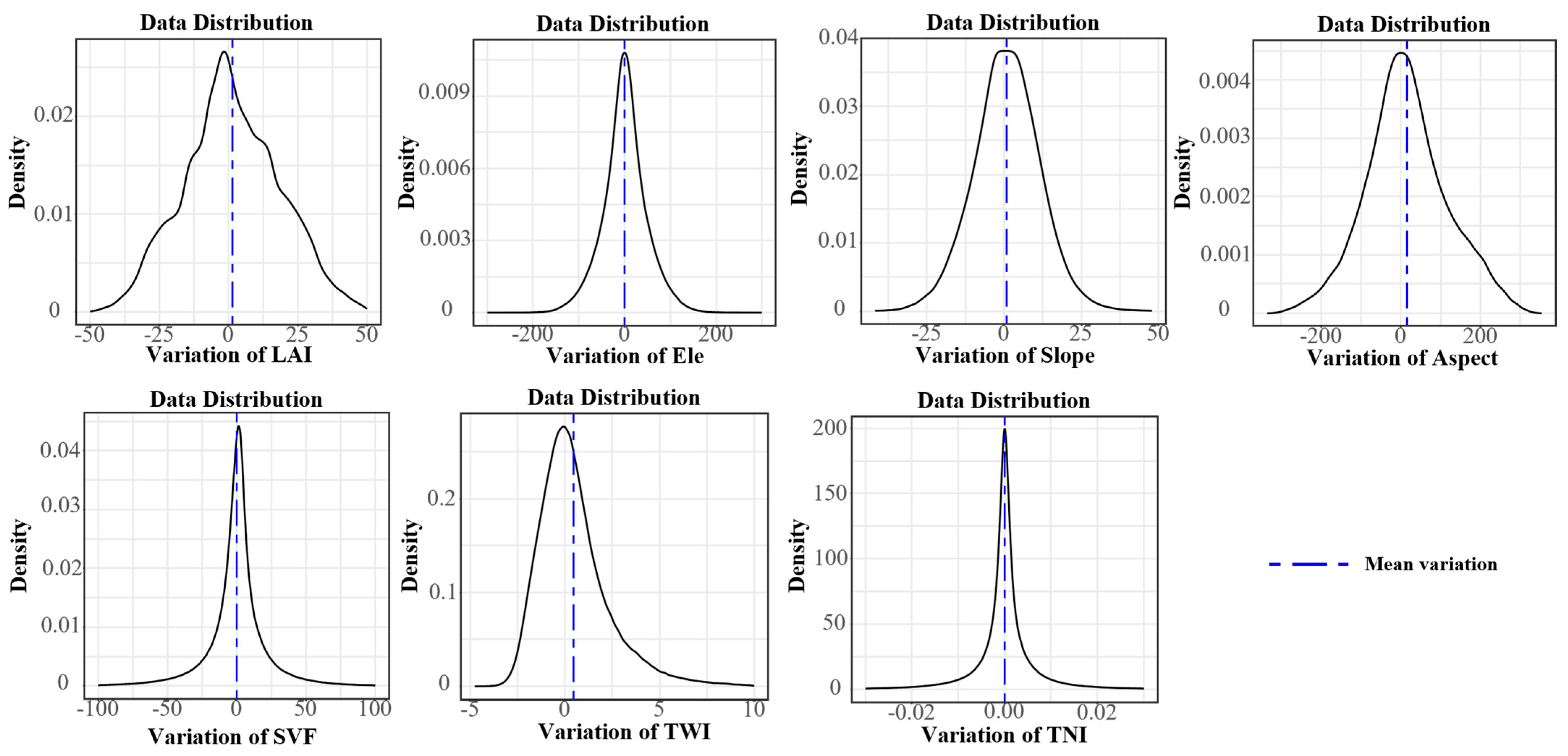
Overall, all ML-based GPP upscaling error correction methods comprise two primary steps: (1) simulating and predicting errors across scales and (2) removing upscaling errors from coarse-resolution GPP products. Given that step 2 can be achieved through simple differencing, the key to improving calibration accuracy lies in enhancing the simulation and prediction capabilities of machine learning models. This enhancement primarily involves adopting advanced algorithms and optimizing training sample quality. While the simulation performance of established machine learning algorithms has been extensively validated with marginal inter-algorithm differences, this study focuses on refining training samples to boost model efficacy. Through in-depth analysis of surface heterogeneity transitions during upscaling, we introduce tailored geostatistical methods to quantitatively characterize these dynamics. This approach improves training sample representativeness, strengthens model simulation-prediction performance, and ultimately achieves superior error correction outcomes. Simultaneously, our approach circumvents the subjective threshold setting employed in prior studies, which often causes calibration accuracy fluctuations, thereby achieving enhanced stability and reliability in calibration performance. Figure 10 illustrates that previous studies achieved notably better correction accuracy when using LAI and SVF alone than other factors. This disparity is attributed to the concentrated distribution of their sub-pixel values within narrow ranges (−50, 50) and (−25, 25), respectively, with most values centered around 0. Conversely, elevation and TWI exhibited broader distributions within ranges like (−100, 100) and (−2.5, 5), respectively. Previous studies set extensive statistical intervals (e.g., (−200, 200) for elevation), adversely affecting correction accuracy. Slope, with distribution mainly within (−25°, 25°), suffered from overly large steps (e.g., step = 15), insufficiently capturing the values near 0 and leading to suboptimal correction. In contrast, the statistical intervals derived from the optimal-step equidistant sampling method or k-means clustering method aligned closely with the primary distribution ranges of surface heterogeneities. These methods effectively captured the main distribution characteristics of surface heterogeneities by selecting appropriate steps, significantly enhancing correction accuracy. This underscores the importance of considering nonuniform density distributions of surface heterogeneities in spatial scaling algorithms.

4.2. Influence of Interval Number on the Correction Accuracy of the Equidistant Sampling Method and K-Means Clustering Method

By incrementally increasing the number of intervals through equidistant division with the optimal step, we analyzed the correction effects of each factor. The results indicated that, when intervals were expanded to eight and ten, factors such as LAI, elevation, and TWI showed improved correction accuracy. Slope and aspect initially saw accuracy gains that later declined, while SVF and TNI exhibited decreased accuracy. As illustrated in Table S7, LAI, elevation, and TWI maintained improved accuracy even with interval expansion, remaining within the primary distribution range of sub-pixel heterogeneities and emphasizing concentrated data distribution around zero. Slope and aspect, although staying within the principal distribution range, experienced weakened capture of concentrated distribution with 10 intervals, leading to initial accuracy gains followed by declines. Conversely, SVF and TNI exceeded the main distribution range post-interval expansion, decreasing accuracy. The performance of each factor was compared with the increased interval using the k-means clustering method. It can be found that LAI, slope, aspect, TWI, and TNI benefitted from increased intervals, enhancing correction accuracy. In contrast, elevation and SVF experienced decreased accuracy, likely due to their broader main distribution range and distinct concentrated distribution characteristics of heterogeneities. These findings underscore the importance of selecting optimal intervals tailored to each factor’s density distribution.
This study also compared the correction effects between the optimal-step equidistant sampling method and the k-means clustering method. As depicted in Table S3, the optimal-step equidistant sampling method consistently outperformed the k-means clustering method when fewer intervals were used. This superiority arises because the density curves of sub-pixel surface heterogeneity exhibit peaks near 0, making the k-means clustering method less effective when the number of categories is insufficient to capture this concentrated distribution, similar to using an excessive step in the equidistant sampling method. In contrast, the optimal-step equidistant sampling method starts from zero and iteratively determines the optimal step on both sides to divide intervals, effectively capturing the characteristics of concentrated distributions and achieving better correction accuracy. Using LAI as an example, this study compared the correction effects of the optimal-step equidistant sampling method and the k-means clustering method when continuously increasing the number of intervals. As shown in Figure 6, with increased intervals, the correction accuracy of the optimal-step equidistant sampling method initially rose and then declined. In contrast, the k-means clustering method showed continuous improvement followed by stabilization. When the interval ranges did not exceed the primary distribution range of surface heterogeneities, the optimal-step equal interval method demonstrated improved accuracy; however, accuracy decreased when the range was exceeded. The k-means clustering method, by subdividing intervals with an increasing number, better captured the concentrated distributions, resulting in improved accuracy. Yet, once the intervals were sufficiently subdivided, further increases did not enhance accuracy. Therefore, in the correction process, identifying the optimal number of intervals is crucial for maximizing correction accuracy for both the optimal-step equidistant sampling method and the k-means clustering method. Typically, this study found that setting intervals to 24 achieved similar R2 values for both methods, specifically 0.773 for the optimal-step equidistant sampling method and 0.763 for the k-means clustering method, demonstrating comparable correction effectiveness.

4.3. Contribution of Heterogeneity Factors in Correction

This study evaluated the contributions of various factors to calibration accuracy through a series of single-factor and multi-factor combined correction experiments. As illustrated in Figure 3, in single-factor correction experiments, the ranking of calibration accuracy from highest to lowest was elevation, slope, LAI, aspect, SVF, land cover, TNI, and TWI. Multi-factor combined experiments demonstrated that integrating vegetation and topographic heterogeneity could enhance calibration accuracy. However, it was observed that incorporating the derived index TWI in combined correction led to lower accuracy compared to combinations excluding TWI. This could be attributed to TWI’s poorer performance in single-factor correction, which added redundant data in the combined correction, thereby reducing overall model fitting and calibration accuracy. Conversely, the inclusion of TNI, which performed closer to other factors in single-factor correction, resulted in a slight improvement in accuracy during combined correction. Hence, while multi-factor combined correction effectively enhances accuracy, selecting factors should be optimized based on specific conditions rather than including more factors indiscriminately.
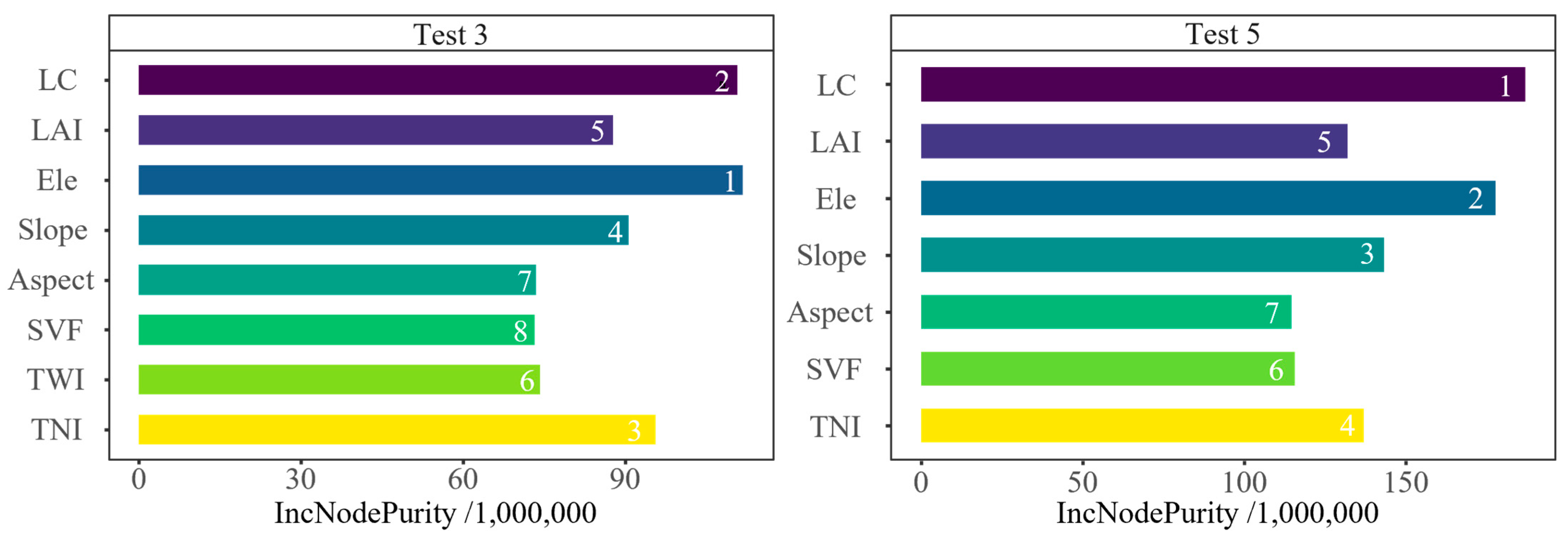
This study employed the random forest algorithm to assess the contribution of factors in multi-factor combined correction. As depicted in Figure 11, Test 3 and Test 5 represented combinations with and without TWI, respectively. Land cover, elevation, slope, and TNI were identified as the most influential factors, followed by LAI, whereas aspect, SVF, and TWI exhibited comparable importance. Land cover influences vegetation type and density, directly impacting parameters like maximum light use efficiency (LUE), carboxylation rate, and leaf clumping. LAI describes vegetation canopy structure, which is crucial for vegetation–atmosphere interactions. In mountainous regions, elevation and slope play critical roles in water redistribution, affecting GPP spatial distribution. TNI and TWI quantify elevation and slope impacts on topography, reflecting microclimatic water and heat characteristics essential for vegetation growth and indirectly influencing GPP spatial patterns.
It is important to note that, while random forest provides feature importance based on data partitioning error reduction, it does not explain individual prediction’s contributions. Therefore, its feature importance ranking serves as a general guide rather than an exhaustive explanation of each factor’s role in the final output. The multi-factor combined experiments in this study categorized factors broadly into vegetation, topographic, and specific combinations, revealing insights such as the superior performance of vegetation heterogeneity factors alone over topographic factors alone and the higher calibration accuracy using TNI compared to TWI. Future studies could explore all possible factor combinations or employ SHAP (SHapley Additive exPlanations) methods to explain each factor’s contribution in machine learning models. By integrating multiple methodologies, a deeper understanding of each factor’s performance in the calibration process could be achieved.

4.4. Residual Correction Error Analysis

The 16 selected mountainous watersheds in this study encompass prevalent vegetation types, with an elevation range of 73–4000 m covering complex topographic conditions from flat to steep and rugged terrain. This effectively validates both the correction performance and transferability of the proposed method. To thoroughly investigate the strengths and limitations of the method across different scenarios, we evaluated residual correction errors using the median absolute error (MedAE) from both vegetation and topographic perspectives. The calculation formulas are as follows:
M e d A E y a , y a ^ = m e d i a n y a y a ^ , , y n y n ^
where y a and y a ^ denote the corrected value and true value of pixel a, respectively. y n and y n ^ denote the corrected value and true value of pixel n, respectively. MedAE was calculated separately for distinct land cover types, LAI intervals, elevation zones, and slope ranges, where lower MedAE values indicate superior correction performance under the given conditions.
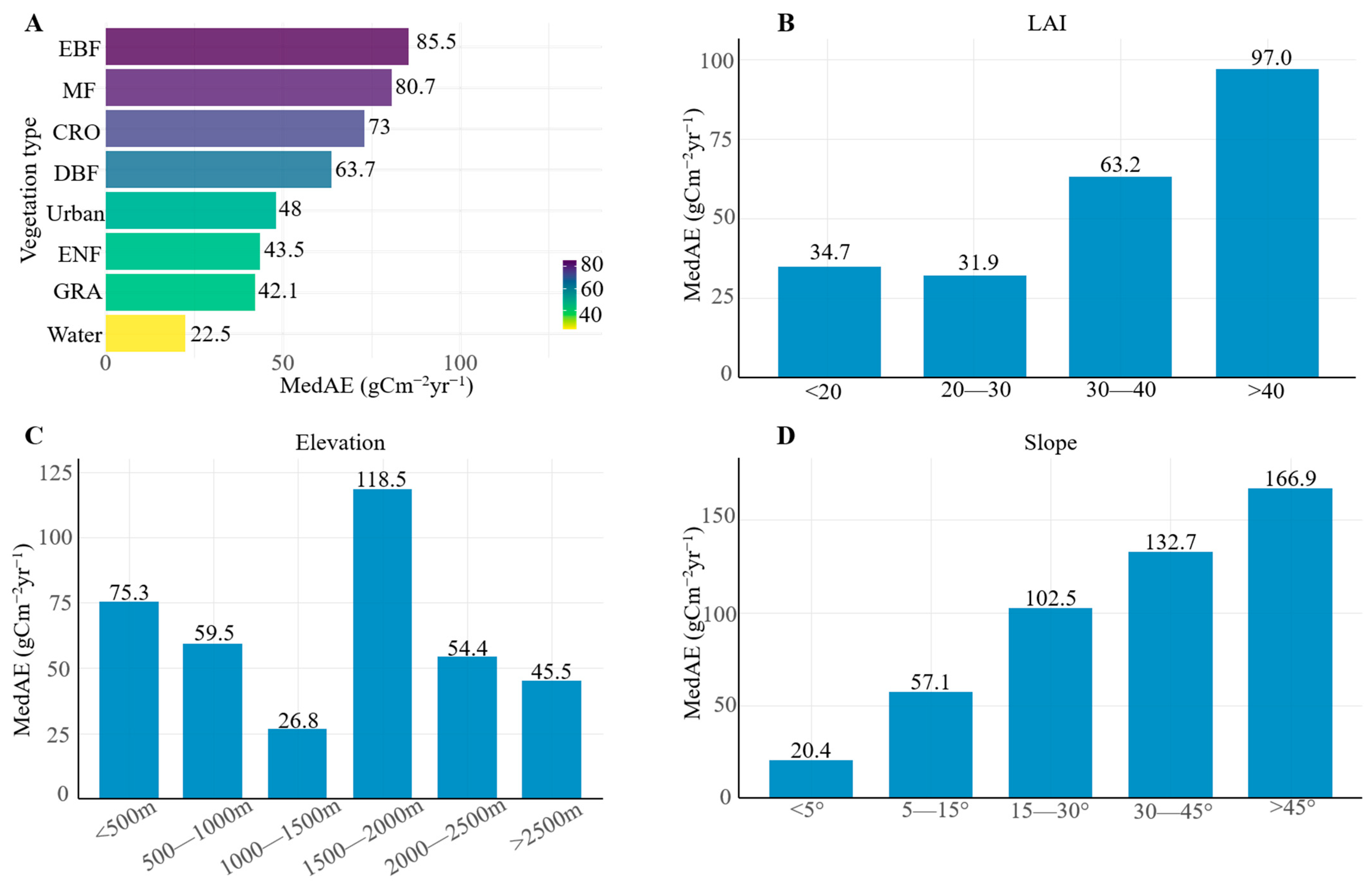
As illustrated in Figure 12, water and grasslands exhibited the most homogeneous characteristics and consequently achieved optimal correction results. Conversely, the poorest correction performance occurred in evergreen broadleaf forests due to vertical canopy-induced “radiation deprivation effects,” mixed forests because of “niche compression” from interspecies light competition, croplands owing to intensive anthropogenic interventions, and deciduous broadleaf forests resulting from phenological abruptness [37,38]. Evergreen needleleaf forests and urban areas showed moderate correction efficacy, attributable to “photosynthetic saturation hysteresis” and complex multi-stress environments, respectively. Regarding LAI, optimal correction occurred at the range 20–30, likely because this interval corresponds to mature forest canopies with peak photosynthetic efficiency and stable remote sensing signals. The poorest performance emerged at LAI > 40, which may reflect suppressed photosynthetic contributions from understory vegetation and topographic shadowing effects.
For elevation, the 1000–1500 m zone demonstrated the best performance, typically representing an optimal hydrothermal equilibrium zone that avoids low-elevation drought and high-altitude cold stress, with canopy structures favorable for ecological parameter estimation [39]. The weakest correction occurred at 1500–2000 m, potentially due to topography–climate mismatches where temperature abruptness shortens growing seasons, impairing GPP estimation [40]. On slopes < 5°, flat terrain exhibited optimal correction owing to uniform radiation, stable soil conditions, and vegetation homogeneity. Conversely, steep slopes > 45° showed the poorest performance due to canopy shadowing and rapid water loss. Collectively, the proposed method delivers the highest correction accuracy for mid-elevation mature forest canopies and the lowest for high-LAI areas at mid-to-high elevations, with acceptable precision in other scenarios. Future research should prioritize mitigating the impacts of steep topography and abrupt temperature shifts while addressing high-LAI interference to further optimize the method for complex mountainous environments.

5. Summary

This study incorporates geostatistical methods, including equidistant sampling and k-means clustering, into the ML-based GPP upscaling error correction framework. This approach quantitatively characterizes dynamic surface heterogeneity variations during upscaling processes, improves training sample representativeness, and effectively enhances GPP upscaling error correction accuracy. Through comprehensive experiments, the following conclusions were obtained:
(1)
Compared with conventional approaches using elevation alone for error correction (R2 of 0.48 and RMSE of 285 gCm−2yr−1), the implementation of the equidistant sampling method with optimal step size and intervals improved R2 by 0.27 and decreased RMSE by 91.22 gCm−2yr−1. Similarly, the application of the K-means clustering method enhanced R2 by 0.21 and reduced RMSE by 63.54 gCm−2yr−1.
(2)
When employing an identical number of statistical intervals, the equidistant sampling method with optimal step size consistently outperforms the k-means clustering approach. Using LAI calibration as an example, only when the number of intervals reaches 24 can the k-means clustering method match the accuracy of the optimal-step equidistant sampling method, with R2 values of 0.763 vs. 0.773 and RMSE values of 194.33 and 190.10 gCm−2yr−1, respectively. The optimal-step equidistant sampling method, paired with appropriate interval selection, offers an efficient solution that maintains high correction accuracy while minimizing computational costs.
(3)
Land cover, elevation, slope, and TNI were identified as the most influential factors, followed by LAI, whereas aspect, SVF, and TWI exhibited comparable importance.
In conclusion, this study underscores the importance of understanding and effectively capturing the nonuniform density distributions of surface heterogeneities in calibration processes. Utilizing methods like the optimal-step equidistant sampling method and carefully selecting factors for multi-factor combined calibration can significantly improve the accuracy of error correction.

Supplementary Materials

The following supporting information can be downloaded at: https://www.mdpi.com/article/10.3390/rs18010023/s1. References [41,42,43,44,45,46,47,48,49,50,51,52,53,54,55,56] are cited in the Supplementary Materials.

Author Contributions

Conceptualization, X.X.; Methodology, Z.W. and X.X.; Software, J.Z.; Validation, J.Z.; Formal Analysis, J.Z. and Z.Y.; Investigation, J.Z.; Data Curation, J.Z. and X.X.; Writing—Original Draft Preparation, J.Z. and Z.W.; Visualization, J.Z.; Writing—review & editing, Z.W. and X.X.; All authors have read and agreed to the published version of the manuscript.

Funding

This study has been jointly supported by the National Key Research and Development Program of China (2024YFF1306503), the National Natural Science Foundation of China (42201418, 42471429), Science and Technology Cooperation Project of CNPC-SWPU Innovation Alliance (2020CX020303), Sichuan Science and Technology Program (2023YFS0406, 2024NSFSC0794, 24YFHZ0133), and the Chinese Academy of Sciences Youth Innovation Promotion Association (2023390).

Data Availability Statement

We extend our thanks to all the data providers. The meteorological data and EC data are available at the global FLUXNET website (http://daac.ornl.gov/fluxnet/). The DEM and Landsat data are available at the USGS website (https://ers.cr.usgs.gov/). The LC and soil texture maps are available at the FROM-GLC center (http://data.ess.tsinghua.edu.cn) and the Open Land Map center (https://openlandmap.org), respectively.

Conflicts of Interest

The authors declare no conflicts of interest.

References

  1. Reichstein, M.; Camps-Valls, G.; Stevens, B.; Jung, M.; Denzler, J.; Carvalhais, N.; Prabhat. Deep learning and process understanding for data-driven Earth system science. Nature 2019, 566, 195–204. [Google Scholar] [CrossRef] [PubMed]
  2. Schimel, D.; Pavlick, R.; Fisher, J.B.; Asner, G.P.; Saatchi, S.; Townsend, P.; Miller, C.; Frankenberg, C.; Hibbard, K.; Cox, P. Observing terrestrial ecosystems and the carbon cycle from space. Glob. Change Biol. 2015, 21, 1762–1776. [Google Scholar] [CrossRef] [PubMed]
  3. Hu, Z.; Shi, H.; Cheng, K.; Wang, Y.-P.; Piao, S.; Li, Y.; Zhang, L.; Xia, J.; Zhou, L.; Yuan, W.; et al. Joint structural and physiological control on the interannual variation in productivity in a temperate grassland: A data-model comparison. Glob. Change Biol. 2018, 24, 2965–2979. [Google Scholar] [CrossRef]
  4. Yuan, W.; Lin, S.; Wang, X. Progress of studies on satellite-based terrestrial vegetation production models in China. Progress. Phys. Geogr.-Earth Environ. 2022, 46, 889–908. [Google Scholar] [CrossRef]
  5. Xie, X.Y.; Li, A.N.; Chen, J.M.; Guan, X.B.; Leng, J.Y. Quantifying Scaling Effect on Gross Primary Productivity Estimation in the Upscaling Process of Surface Heterogeneity. J. Geophys. Res. Biogeosci. 2022, 127, e2021JG006775. [Google Scholar] [CrossRef]
  6. Lawrence, D.M.; Fisher, R.A.; Koven, C.D.; Oleson, K.W.; Swenson, S.C.; Bonan, G.; Collier, N.; Ghimire, B.; van Kampenhout, L.; Kennedy, D.; et al. The Community Land Model Version 5: Description of New Features, Benchmarking, and Impact of Forcing Uncertainty. J. Adv. Model. Earth Syst. 2019, 11, 4245–4287. [Google Scholar] [CrossRef]
  7. Tesfa, T.K.; Leung, L.-Y.R. Exploring new topography-based subgrid spatial structures for improving land surface modeling. Geosci. Model Dev. 2017, 10, 873–888. [Google Scholar] [CrossRef]
  8. Chen, J.M.; Chen, X.; Ju, W. Effects of vegetation heterogeneity and surface topography on spatial scaling of net primary productivity. Biogeosciences 2013, 10, 4879–4896. [Google Scholar] [CrossRef]
  9. Xie, X.; Chen, J.M.; Gong, P.; Li, A. Spatial Scaling of Gross Primary Productivity Over Sixteen Mountainous Watersheds Using Vegetation Heterogeneity and Surface Topography. J. Geophys. Res. Biogeosci. 2021, 126, e2020JG005848. [Google Scholar] [CrossRef]
  10. Dang, C.Y.; Shao, Z.F.; Huang, X.; Qian, J.X.; Cheng, G.; Ding, Q.; Fan, Y.W. Assessment of the importance of increasing temperature and decreasing soil moisture on global ecosystem productivity using solar-induced chlorophyll fluorescence. Glob. Change Biol. 2022, 28, 2066–2080. [Google Scholar] [CrossRef] [PubMed]
  11. Stocker, B.D.; Zscheischler, J.; Keenan, T.F.; Prentice, I.C.; Seneviratne, S.I.; Peñuelas, J. Drought impacts on terrestrial primary production underestimated by satellite monitoring. Nat. Geosci. 2019, 12, 264–270. [Google Scholar] [CrossRef]
  12. Stoy, P.C.; Mauder, M.; Foken, T.; Marcolla, B.; Boegh, E.; Ibrom, A.; Arain, M.A.; Arneth, A.; Aurela, M.; Bernhofer, C.; et al. A data-driven analysis of energy balance closure across FLUXNET research sites: The role of landscape scale heterogeneity. Agric. For. Meteorol. 2013, 171–172, 137–152. [Google Scholar] [CrossRef]
  13. Moorcroft, P.R.; Hurtt, G.C.; Pacala, S.W. A Method for Scaling Vegetation Dynamics: The Ecosystem Demography Model (ED). Ecol. Monogr. 2001, 71, 557–585. [Google Scholar] [CrossRef]
  14. Chen, C.; Hu, B.; Li, Y. Easy-to-use spatial random-forest-based downscaling-calibration method for producing precipitation data with high resolution and high accuracy. Hydrol. Earth Syst. Sci. 2021, 25, 5667–5682. [Google Scholar] [CrossRef]
  15. Kirboga, K.K.; Kucuksille, E.U.; Naldan, M.E.; Isik, M.; Gulcu, O.; Aksakal, E. CVD22: Explainable artificial intelligence determination of the relationship of troponin to D-Dimer, mortality, and CK-MB in COVID-19 patients. Comput. Methods Programs Biomed. 2023, 233, 107492. [Google Scholar] [CrossRef]
  16. Fathololoumi, S.; Firozjaei, M.K.; Biswas, A. Improving spatial resolution of satellite soil water index (SWI) maps under clear-sky conditions using a machine learning approach. J. Hydrol. 2022, 615, 128709. [Google Scholar] [CrossRef]
  17. Mohammady, M.; Pourghasemi, H.R.; Amiri, M. Land subsidence susceptibility assessment using random forest machine learning algorithm. Environ. Earth Sci. 2019, 78, 503. [Google Scholar] [CrossRef]
  18. Songlin, C.; Tianxing, W. Comparison Analyses of Equal Interval Method and Mean-standard Deviation Method Used to Delimitate Urban Heat Island. J. Geo-Inf. Sci. 2009, 11, 145–150. [Google Scholar]
  19. Van Arkel, Z.; Kaleita, A.L. Identifying sampling locations for field-scale soil moisture estimation using K-means clustering. Water Resour. Res. 2015, 50, 7050–7057. [Google Scholar] [CrossRef]
  20. Liu, J.; Chen, J.M.; Cihlar, J.; Chen, W. Net primary productivity distribution in the BOREAS region from a process model using satellite and surface data. J. Geophys. Res. Atmos. 1999, 104, 27735–27754. [Google Scholar] [CrossRef]
  21. Leng, J.Y.; Chen, J.M.; Li, W.Y.; Luo, X.Z.; Xu, M.Z.; Liu, J.; Wang, R.; Rogers, C.; Li, B.L.; Yan, Y.L. Global datasets of hourly carbon and water fluxes simulated using a satellite-based process model with dynamic parameterizations. Earth Syst. Sci. Data 2024, 16, 1283–1300. [Google Scholar] [CrossRef]
  22. Chen, J.M.; Chen, X.Y.; Ju, W.M.; Geng, X.Y. Distributed hydrological model for mapping evapotranspiration using remote sensing inputs. J. Hydrol. 2005, 305, 15–39. [Google Scholar] [CrossRef]
  23. Gong, P.; Wang, J.; Yu, L.; Zhao, Y.C.; Zhao, Y.Y.; Liang, L.; Niu, Z.G.; Huang, X.M.; Fu, H.H.; Liu, S.; et al. Finer resolution observation and monitoring of global land cover: First mapping results with Landsat TM and ETM+ data. Int. J. Remote Sens. 2013, 34, 2607–2654. [Google Scholar] [CrossRef]
  24. Cao, R.Y.; Chen, Y.; Shen, M.G.; Chen, J.; Zhou, J.; Wang, C.; Yang, W. A simple method to improve the quality of NDVI time-series data by integrating spatiotemporal information with the Savitzky-Golay filter. Remote Sens. Environ. 2018, 217, 244–257. [Google Scholar] [CrossRef]
  25. Liu, M.; Yang, W.; Zhu, X.L.; Chen, J.; Chen, X.H.; Yang, L.Q.; Helmer, E.H. An Improved Flexible Spatiotemporal DAta Fusion (IFSDAF) method for producing high spatiotemporal resolution normalized difference vegetation index time series. Remote Sens. Environ. 2019, 227, 74–89. [Google Scholar] [CrossRef]
  26. Deng, F.; Chen, J.M.; Plummer, S.; Chen, M.Z.; Pisek, J. Algorithm for global leaf area index retrieval using satellite imagery. IEEE Trans. Geosci. Remote Sens. 2006, 44, 2219–2229. [Google Scholar] [CrossRef]
  27. van Zyl, J.J. The Shuttle Radar Topography Mission (SRTM): A breakthrough in remote sensing of topography. Acta Astronaut. 2001, 48, 559–565. [Google Scholar] [CrossRef]
  28. Sorensen, R.; Zinko, U.; Seibert, J. On the calculation of the topographic wetness index: Evaluation of different methods based on field observations. Hydrol. Earth Syst. Sci. 2006, 10, 101–112. [Google Scholar] [CrossRef]
  29. Zaksek, K.; Ostir, K.; Kokalj, Z. Sky-View Factor as a Relief Visualization Technique. Remote Sens. 2011, 3, 398–415. [Google Scholar] [CrossRef]
  30. Hutengs, C.; Vohland, M. Downscaling land surface temperatures at regional scales with random forest regression. Remote Sens. Environ. 2016, 178, 127–141. [Google Scholar] [CrossRef]
  31. Zhao, W.; Duan, S.-B.; Li, A.; Yin, G. A practical method for reducing terrain effect on land surface temperature using random forest regression. Remote Sens. Environ. 2019, 221, 635–649. [Google Scholar] [CrossRef]
  32. Macqueen, J. Some Methods for Classification and Analysis of MultiVariate Observations. In Proceedings of the Fifth Berkeley Symposium on Mathematical Statistics and Probability; University of California Press: Oakland, CA, USA, 1967; Volume 1. [Google Scholar]
  33. Celebi, M.E.; Kingravi, H.A.; Vela, P.A. A comparative study of efficient initialization methods for the k-means clustering algorithm. Expert. Syst. Appl. 2013, 40, 200–210. [Google Scholar] [CrossRef]
  34. Govind, A.; Chen, J.M.; Margolis, H.; Ju, W.; Sonnentag, O.; Giasson, M.-A. A spatially explicit hydro-ecological modeling framework (BEPS-TerrainLab V2.0): Model description and test in a boreal ecosystem in Eastern North America. J. Hydrol. 2009, 367, 200–216. [Google Scholar] [CrossRef]
  35. El Maayar, M.; Chen, J.M. Spatial scaling of evapotranspiration as affected by heterogeneities in vegetation, topography, and soil texture. Remote Sens. Environ. 2006, 102, 33–51. [Google Scholar] [CrossRef]
  36. Hao, D.; Bisht, G.; Huang, M.; Ma, P.-L.; Tesfa, T.; Lee, W.-L.; Gu, Y.; Leung, L.R. Impacts of Sub-Grid Topographic Representations on Surface Energy Balance and Boundary Conditions in the E3SM Land Model: A Case Study in Sierra Nevada. J. Adv. Model. Earth Syst. 2022, 14, e2021MS002862. [Google Scholar] [CrossRef]
  37. Zhu, W.; Zhao, C.; Xie, Z. An End-to-End Satellite-Based Gpp Estimation Model Devoid of Meteorological and Land Cover Data. Agric. For. Meteorol. 2023, 331, 109337. [Google Scholar] [CrossRef]
  38. Xie, X.; Zhao, W.; Yin, G.; Fu, H.; Wang, X. Divergent Ecological Restoration Driven by Afforestation Along the North and South Banks of the Yarlung Zangbo Middle Reach. Land Degrad. Dev. 2025, 36, 521–532. [Google Scholar] [CrossRef]
  39. Zuo, X.; Xu, K.; Zhao, P.; Wang, X.; Han, H. Influence of Mountain Shadows on Forest-Dominant Tree Species Mapping and Its Response to Topographic Corrections. For. Sci. 2025, 71, 625–656. [Google Scholar] [CrossRef]
  40. Cheng, Z.; Chen, J.M.; Guo, Z.; Miao, G.; Zeng, H.; Wang, R.; Huang, Z.; Wang, Y. Improving UAV-Based LAI Estimation for Forests Over Complex Terrain by Reducing Topographic Effects on Multispectral Reflectance. IEEE Trans. Geosci. Remote Sens. 2024, 62, 1–19. [Google Scholar] [CrossRef]
  41. Matsumoto, K.; Ohta, T.; Nakai, T.; Kuwada, T.; Daikoku, K.I.; Iida, S.I.; Yabuki, H.; Kononov, A.V.; Molen, M.K.V.D.; Kodama, Y. Energy consumption and evapotranspiration at several boreal and temperate forests in the Far East. Agric. For. Meteorol. 2008, 148, 1978–1989. [Google Scholar] [CrossRef]
  42. Zielis, S.; Etzold, S.; Zweifel, R.; Eugster, W.; Haeni, M.; Buchmann, N. NEP of a Swiss subalpine forest is significantly driven not only by current but also by previous year’s weather. Biogeosciences 2014, 11, 1627–1635. [Google Scholar] [CrossRef]
  43. Acosta, M.; Pavelka, M.; Montagnani, L.; Kutsch, W.; Lindroth, A.; Juszczak, R.A.; Janouš, D. Soil surface CO2 efflux measurements in Norway spruce forests: Comparison betweenfour different sites across Europe—From boreal to alpine forest. Geoderma 2013, 192, 295–303. [Google Scholar] [CrossRef]
  44. Lindauer, M.; Schmid, H.P.; Grote, R.; Mauder, M.; Steinbrecher, R.; Wolpert, B. Net ecosystem exchange over a non-cleared wind-throw-disturbed upland spruce forest—Measurements and simulations. Agric. For. Meteorol. 2014, 197, 219–234. [Google Scholar] [CrossRef]
  45. Marcolla, B.; Pitacco, A.; Cescatti, A. Canopy Architecture and Turbulence Structure in a Coniferous Forest. Bound.-Layer Meteorol. 2003, 108, 39–59. [Google Scholar] [CrossRef]
  46. Montagnani, L.; Manca, G.; Canepa, E.; Georgieva, E.; Acosta, M.; Feigenwinter, C.; Janous, D.; Kerschbaumer, G.; Lindroth, A.; Minach, L. A new mass conservation approach to the study of CO2 advection in an alpine forest. J. Geophys. Res. Atmos. 2009, 114, D07306. [Google Scholar] [CrossRef]
  47. Baker, B.; Guenther, A.; Greenberg, J.; Goldstein, A.; Fall, R. Canopy fluxes of 2-methyl-3-buten-2-ol over a ponderosa pine forest by relaxed eddy accumulation: Field data and model comparison. J. Geophys. Res. Atmos. 1999, 104, 26107–26114. [Google Scholar] [CrossRef]
  48. Arain, M.A.; Restrepo-Coupe, N. Net ecosystem production in a temperate pine plantation in southeastern Canada. Agric. For. Meteorol. 2005, 128, 223–241. [Google Scholar] [CrossRef]
  49. Campbell, J.L.; Sun, O.J.; Law, B.E. Disturbance and net ecosystem production across three climatically distinct forest landscapes. Glob. Biogeochem. Cycles 2004, 18, GB4017.1–GB4017.11. [Google Scholar] [CrossRef]
  50. Bond-Lamberty, B.; Wang, C.; Gower, S.T. A global relationship between the heterotrophic and autotrophic components of soil respiration? Glob. Change Biol. 2004, 10, 1756–1766. [Google Scholar] [CrossRef]
  51. Anthoni, P.M.; Unsworth, M.H.; Law, B.E.; Irvine, J.; Moore, D. Seasonal differences in carbon and water vapor exchange in young and old-growth ponderosa pine ecosystems. Agric. For. Meteorol. 2002, 111, 203–222. [Google Scholar] [CrossRef]
  52. Ruehr, N.K.; Martin, J.G.; Law, B.E. Effects of water availability on carbon and water exchange in a young ponderosa pine forest: Above- and belowground responses. Agric. For. Meteorol. 2012, 164, 136–148. [Google Scholar] [CrossRef]
  53. Albert, L.P.; Keenan, T.F.; Burns, S.P.; Huxman, T.E.; Monson, R.K. Climate controls over ecosystem metabolism: Insights from a fifteen-year inductive artificial neural network synthesis for a subalpine forest. Oecologia 2017, 184, 25–41. [Google Scholar] [CrossRef]
  54. Aubinet, M.; Chermanne, B.; Vandenhaute, M.; Longdoz, B.; Yernaux, M.; Laitat, E. Long term carbon dioxide exchange above a mixed forest in the Belgian Ardennes. Agric. For. Meteorol. 2001, 108, 293–315. [Google Scholar] [CrossRef]
  55. Etzold, S.; Ruehr, N.K.; Zweifel, R.; Dobbertin, M.; Zingg, A.; Pluess, P.; Häsler, R.; Eugster, W.; Buchmann, N. The Carbon Balance of Two Contrasting Mountain Forest Ecosystems in Switzerland: Similar Annual Trends, but Seasonal Differences. Ecosystems 2011, 14, 1289–1309. [Google Scholar] [CrossRef]
  56. Guan, D.-X.; Wu, J.-B.; Zhao, X.-S.; Han, S.-J.; Yu, G.-R.; Sun, X.-M.; Jin, C.-J. CO2 fluxes over an old, temperate mixed forest in northeastern China. Agr. Forest Meteorol. 2006, 137, 138–149. [Google Scholar] [CrossRef]
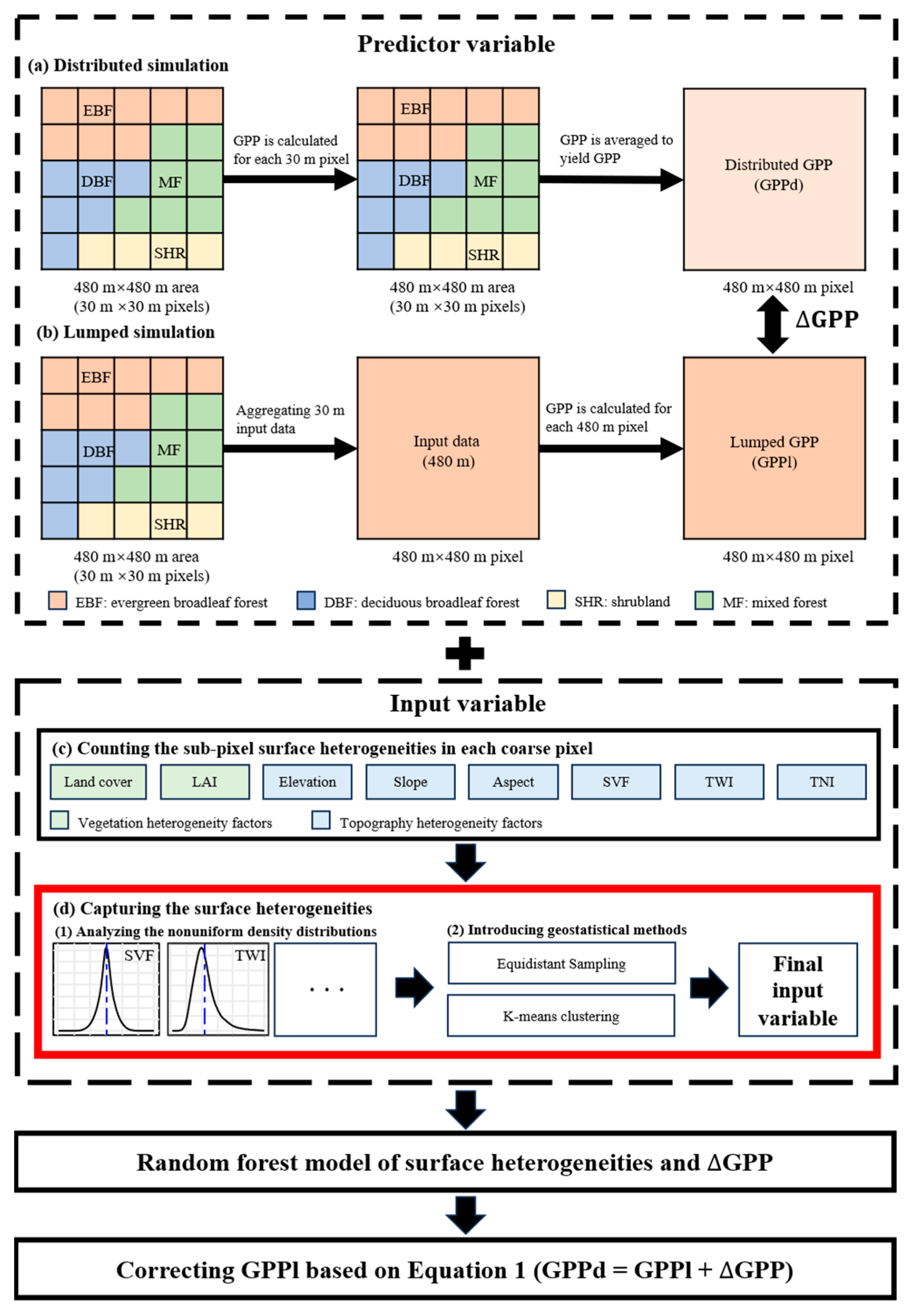
Figure 1. Method flowchart.
Remotesensing 18 00023 g001
Figure 2. Correction effect of dividing 6 equal intervals using different steps. LAI: leaf area index; Ele: elevation; SVF: sky view factor; TWI: topographic wetness index; TNI: terrain niche index.
Remotesensing 18 00023 g002
Figure 3. Sorting of single factor correction effects. None: uncorrected; LAI: leaf area index; Ele: elevation; SVF: sky view factor; TWI: topographic wetness index; TNI: terrain niche index.
Remotesensing 18 00023 g003
Figure 4. Variation in correction accuracy of two methods with the number of intervals. LAI: leaf area index; Ele: elevation; SVF: sky view factor; TWI: topographic wetness index; TNI: terrain niche index. Equal interval represents the optimal-step equidistant sampling method. Clustering represents k-means clustering method.
Remotesensing 18 00023 g004
Figure 5. Correction effects of the optimal-step equidistant sampling method and k-means clustering method under the same number of intervals. LAI: leaf area index; Ele: elevation; SVF: sky view factor; TWI: topographic wetness index; TNI: terrain niche index. (AC) show the comparison of correction accuracy with 6 intervals; (DF) show the comparison of correction accuracy with 8 intervals; (GI) show the comparison of correction accuracy with 10 intervals. Equal interval represents the optimal-step equidistant sampling method. Clustering represents the k-means clustering method.
Remotesensing 18 00023 g005
Figure 6. Variation in correction accuracy of two methods with increasing number of intervals. Equal interval represents the optimal-step equidistant sampling method. Clustering represents the k-means clustering method.
Remotesensing 18 00023 g006
Figure 7. Comparison of correction accuracy among different tests.
Remotesensing 18 00023 g007
Figure 8. Regression between GPPd and GPPl before and after combination corrections. The dashed black line represents a 1:1 linear regression, while the solid red line represents the best linear regression. (A) shows the performance of the control group; (BG) show the performance of test 1–6, respectively.
Remotesensing 18 00023 g008
Figure 9. Comparison before and after calibration of a single site. (AC) The effects before, reference, and after calibration of station 109, respectively. (DF) The effects before, reference, and after calibration of station 158, respectively.
Remotesensing 18 00023 g009
Figure 10. Density curves of the surface heterogeneity. LAI: leaf area index; Ele: elevation; SVF: sky view factor; TWI: topographic wetness index; TNI: terrain niche index.
Remotesensing 18 00023 g010
Figure 11. Importance ranking based on random forest. LAI: leaf area index; Ele: elevation; SVF: sky view factor; TWI: topographic wetness index; TNI: terrain niche index.
Remotesensing 18 00023 g011
Figure 12. Median absolute error of different vegetation types and terrain conditions. (AD) The median absolute errors corresponding to different vegetation types, leaf area indices, elevations, and slopes, respectively. EBF: evergreen broadleaf forests; MF: mixed forests; CRO: croplands; DBF: deciduous broadleaf forests; ENF: evergreen needleleaf forests; GRA: grasslands; LAI: leaf area index.
Remotesensing 18 00023 g012
Table 1. Parameter setting experiments.
MethodExperimentParameter SettingExperimental Purpose
Equidistant sampling IThe step: the value incremented from 0 (e.g., set the step to 10, 20, 30, 40, respectively).
The number of intervals: 6.
(a)
Analyzing the impact of steps on calibration accuracy.
(b)
Identifying the optimal step.
IIThe step: the optimal step identified in experiment I.
The number of intervals: 6, 8, 10, respectively.
Analyzing the calibration accuracy of increasing intervals appropriately.
K-means clustering IIIThe categories: 6, 8, 10, respectively (the corresponding intervals are 6, 8, 10).
(a)
Testing the effect of appropriately increasing the number of intervals on calibration accuracy.
(b)
Comparing the results with the equal interval method in Experiment II.
Equidistant sampling/K-means clusteringIVK-means clustering method: the categories are set from 6 to 36 (the corresponding intervals are from 6 to 36).
Equal interval method: the step is set to the optimal step, and the number of intervals is set from 6 to 36.
Testing the performance of the two methods when a sufficient or an excessive number of intervals is set.
Table 2. Description of control tests.
Test GroupDescriptionFactor Combination
Control groupNone
Test 1Vegetation heterogeneitiesLC + LAI
Test 2Topographic heterogeneitiesEle + Slope + Aspect + SVF + TWI + TNI
Test 3All surface heterogeneitiesLC + LAI + Ele + Slope + Aspect + SVF + TWI + TNI
Test 4Without TWI and TNILC + LAI + Ele + Slope + Aspect + SVF
Test 5Without TWILC + LAI + Ele + Slope + Aspect + SVF + TNI
Test 6Without TNILC + LAI + Ele + Slope + Aspect + SVF + TWI
LC: land cover; LAI: leaf area index; Ele: elevation; SVF: sky view factor; TWI: topographic wetness index; TNI: terrain niche index.
Table 3. Comparison of correction accuracy between previous research (PR) and this work (TW).
AccuracyLAIEleSlopeSVFTWI
PRTWPRTWPRTWPRTWPRTW
R20.570.7560.480.7510.50.760.570.7410.450.683
RMSE (gCm−2yr−1)259197285193.8280195.3259202.8294231.1
LAI: leaf area index; Ele: elevation; SVF: sky view factor; TWI: topographic wetness index.
Disclaimer/Publisher’s Note: The statements, opinions and data contained in all publications are solely those of the individual author(s) and contributor(s) and not of MDPI and/or the editor(s). MDPI and/or the editor(s) disclaim responsibility for any injury to people or property resulting from any ideas, methods, instructions or products referred to in the content.