Oilseed Flax Yield Prediction in Arid Gansu, China Using a CNN–Informer Model and Multi-Source Spatio-Temporal Data

Highlights

What are the main findings?

• A CNN–Informer hybrid model is developed to integrate multi-source spatiotemporal data (remote sensing, meteorological, soil, and historical yields), combining convolutional local feature extraction with ProbSparse attention for efficient long-range dependency modeling.
• Comparative experiments demonstrate that the proposed model significantly outperforms representative baselines (LSTM, CNN, Transformer, Informer, and XGBoost), achieving R² = 0.82, RMSE = 0.31 t/ha, MAE = 0.21 t/ha, and MAPE = 10.33%, representing an average improvement of 10–35% across metrics.

What are the implications of the main findings?

• Cross-county fivefold validation and feature ablation confirm strong spatial generalization and robustness, indicating the model’s applicability for county-level yield prediction in arid and semi-arid regions.
• Analysis of feature contributions highlights the dominant role of historical yield and remote sensing indices, while soil and meteorological variables improve spatial differentiation, providing actionable insights for precision crop management and data-driven decision-making.

Abstract

Oilseed flax (Linum usitatissimum, L.) is an important specialty oilseed crop cultivated in arid and semi-arid regions, where timely, accurate yield prediction is crucial for regional oilseed security and agricultural decision-making. To address the lack of robust county-level yield prediction models for oilseed flax, this study proposes a CNN–Informer hybrid framework that integrates convolutional neural networks (CNNs) with the Informer architecture to model multi-source spatio-temporal data. Unlike conventional Transformer-based approaches, the proposed framework combines CNN-based local temporal feature extraction with the ProbSparse attention mechanism of Informer, enabling the efficient modeling of long-range temporal dependencies across multiple years while reducing the computational burden of attention-based time-series modeling. The model incorporates multi-source inputs, including remote sensing indices (NDVI, EVI, SAVI, KNDVI), TerraClimate meteorological variables, soil properties, and historical yield records. Comprehensive experiments conducted at the county level in Gansu Province, China, demonstrate that the CNN–Informer model consistently outperforms representative machine learning and deep learning baselines (Transformer, Informer, LSTM, and XGBoost), achieving an average performance of R² = 0.82, RMSE = 0.31 t/ha, MAE = 0.21 t/ha, and MAPE = 10.33%. Results from feature ablation and historical yield window analyses reveal that a three-year historical yield window yields optimal performance, with remote sensing features contributing most strongly to predictive accuracy, while meteorological and soil variables enhance spatial adaptability under heterogeneous environmental conditions. Model robustness was further verified through fivefold county-based spatial cross-validation, indicating stable performance and strong generalization capability in unseen regions. Overall, the proposed CNN–Informer framework provides a reliable and interpretable solution for county-level oilseed flax yield prediction and offers practical insights for precision management of specialty crops in arid and semi-arid regions.

1. Introduction

Agricultural production is instrumental in driving global economic progress and safeguarding food security. Under increasing pressures from population growth, climate change, and resource constraints, accurate crop yield prediction is essential for sustainable agricultural planning and policy formulation [1]. Flax (Linum usitatissimum L.) is a vital economic crop widely utilized in the production of edible oils, textile fibers, and pharmaceuticals [2]. As the world’s largest consumer of oilseed flax, China accounted for 26.8% of global imports in 2020, with a cumulative import value of approximately USD 31.1 billion over the past decade [3]. Reliable yield forecasting can support planting decisions, reduce production risks, stabilize market supply, and improve the efficiency of the oilseed supply chain [4,5,6], thereby fostering sustainable agricultural economic growth. Crop yield formation is influenced by multiple interacting factors, including soil and meteorological conditions [7,8,9], crop traits, and management practices [10,11,12], resulting in inherently nonlinear relationships between yield and environmental drivers [13]. Existing yield prediction approaches mainly include mechanistic crop models and statistical models [14,15,16,17,18]. Mechanistic models simulate crop growth processes using meteorological, soil, phenological, and management inputs [19], but their applicability at regional scales is often constrained by high data requirements and parameter calibration complexity [20,21,22,23]. Statistical and early remote sensing-based regression models establish empirical relationships between yield and predictor variables [24,25], yet their performance is often unstable due to simplified assumptions and limited ability to represent complex interactions [26]. Although machine learning methods such as decision trees, random forests, and regression-based techniques have been applied to yield prediction, these approaches may still struggle to fully capture nonlinear and multi-factor interactions among environmental variables [27].

In recent years, deep learning technologies have been increasingly applied across agricultural domains due to their strengths in automatic feature extraction, nonlinear modeling, and handling large-scale high-dimensional datasets [28,29,30]. Compared with traditional statistical models and conventional machine learning approaches, deep learning models exhibit higher accuracy and stability in characterizing complex nonlinear relationships and spatio-temporal interactions involved in crop growth processes [30,31,32,33]. Remote sensing technology provides continuous and spatially explicit information on vegetation growth and environmental conditions, thereby significantly improving the timeliness and accuracy of crop yield estimation at regional scales [34]. With rapid advances in sensor technology, remote sensing data with extended temporal coverage and finer spatial resolution—such as MODIS and Sentinel-2—have become increasingly available, enabling detailed monitoring of crop growth dynamics over space and time [35]. Vegetation indices derived from remote sensing data, including the Normalized Difference Vegetation Index (NDVI) and Enhanced Vegetation Index (EVI), have been shown to effectively represent crop growth status and substantially improve yield prediction performance in numerous studies [36,37]. In this context, deep learning approaches combined with multi-source remote sensing data are widely adopted for regional-scale crop yield forecasting. For example, Lu et al. [38] proposed an integrated forecasting framework in China’s Northeast rice-producing regions, combining MODIS and Sentinel-2 data with the WOFOST crop model and deep learning algorithms, which demonstrated significantly higher prediction accuracy compared to traditional machine learning methods. Gavahi, Abbaszadeh, and Moradkhani [32] created a deep yield prediction framework that integrates ConvLSTM and 3D-CNN architectures to effectively model spatio-temporal dependencies in MODIS satellite data, achieving superior predictive capability.

Moreover, Transformer architectures based on attention mechanisms have gained prominence in regional-scale crop yield estimation, offering improvements in both accuracy and interpretability. For instance, Li et al. [39] proposed an AM-CNN-LSTM model that integrates remote sensing indicators such as VTCI, LAI, and FPAR. By incorporating attention mechanisms and uncertainty analysis, their model achieved highly accurate winter wheat yield prediction in the Guanzhong Plain and effectively identified key yield-influencing factors. Similarly, Liu, Wang, Chen, Chen, Wang, Hao and Sun [36] integrated remote sensing time series, environmental variables, and historical yield data into a Transformer-based Informer model for rice yield prediction, achieving substantially enhanced accuracy and interpretability at regional scales through feature importance analysis. Recent studies further demonstrate that Transformer-family models and their variants outperform conventional CNN–LSTM architectures when integrating multi-source satellite time series and modeling heterogeneous agro-environmental conditions [40,41].

Deep learning methods integrated with multi-source data such as remote sensing and meteorology have been extensively applied to predict yields of major food crops including wheat [13,42], rice [33,43,44], and others. These approaches have demonstrated clear advantages in enhancing prediction accuracy and adapting to complex spatio-temporal variability. However, most existing studies have focused on staple crops in relatively homogeneous agroecosystems, with limited attention to oilseed flax, a crop adapted to arid and semi-arid regions. Gansu Province, a key oilseed flax-producing area in northwestern China, features representative dryland agriculture, where cultivation is concentrated in water-limited zones such as the Hexi Corridor and adjacent counties [45]. Yield there is highly sensitive to interannual climate variability—especially precipitation fluctuations and drought intensity, which have intensified under recent climate warming [46,47,48]. Concurrently, marked soil heterogeneity across counties, including differences in texture and organic matter content, affects water-holding capacity and crop stress responses, amplifying spatial variation in yield–environment relationships [49,50]. These region-specific constraints result in strong spatio-temporal nonstationary of county-level yields, underscoring the need for prediction approaches that integrate multi-source data from remote sensing, meteorology, and soil properties to ensure robust performance in heterogeneous dryland systems.

Accordingly, this study proposes a CNN–Informer model for county-level oilseed flax yield prediction in Gansu Province by jointly modeling multi-source spatio-temporal data from remote sensing, meteorology, soil properties, and historical yield records. The main contributions of this study are as follows:

(1)

A county-level yield prediction framework for oilseed flax is established, addressing the underrepresentation of specialty oilseed crops in deep learning–based studies in arid and semi-arid regions.

(2)

The performance of an attention-enhanced CNN–Informer model is evaluated against representative machine learning and deep learning baselines (LSTM, Transformer, Informer, and XGBoost).

(3)

The added value of integrating multi-source data—including remote sensing indices, meteorological variables, soil properties, and historical yields—is systematically assessed using alternative feature combination schemes.

(4)

The spatial and temporal generalization performance of the proposed model is evaluated through county-based five-fold cross-validation with strict year-wise data partitioning.

Overall, this study provides methodological support for robust yield prediction and the digital management of specialty oilseed crops in heterogeneous dryland agroecosystems.

2. Materials and Methods

2.1. Study Area

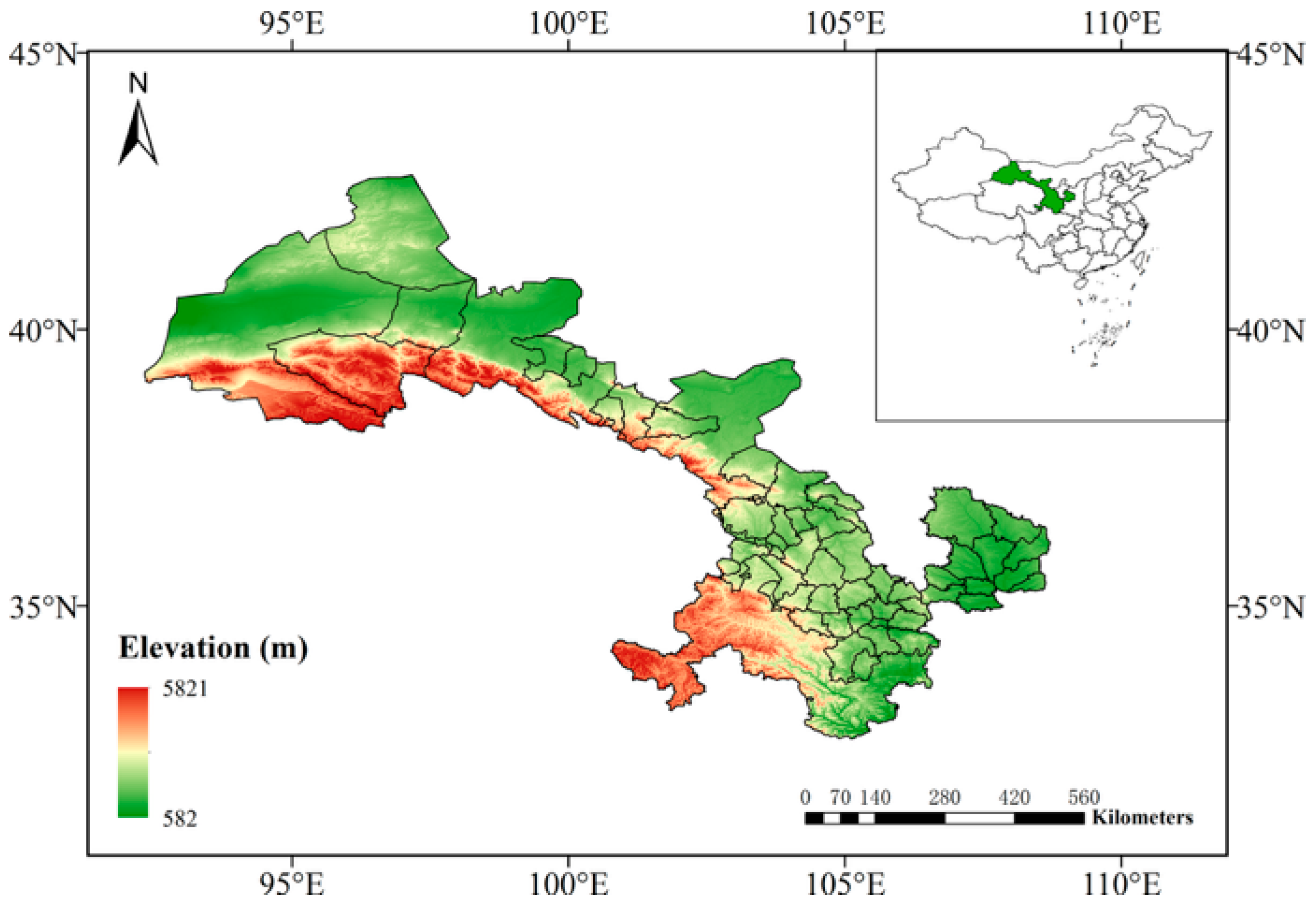
The study area is located in Gansu Province, China, situated in the northwestern region of China (Figure 1), a major oilseed flax-producing region spanning 32°35′–42°57′N and 92°13′–108°46′E, with an area of approximately 454,000 km². The province features complex topography and pronounced environmental heterogeneity, and oilseed flax is widely cultivated across Gansu, with major production areas extending from the Loess Plateau to the arid and semi-arid zones of the Hexi Corridor (e.g., Zhangye, Wuwei, and Jiuquan) and the northern foothills of the Qilian Mountains. Gansu has a typical arid to semi-arid continental climate, with mean annual temperatures ranging from 6 to 14 °C and strong spatial gradients in precipitation, which decreases from about 600 mm in the southeastern Loess Plateau to less than 100 mm in the northwestern arid regions, with most rainfall occurring between June and September. Under these water-limited conditions, soil water stress induces strong interannual variability in crop growth, making timely monitoring of vegetation dynamics and environmental stress essential for accurate modeling of oilseed flax growth and yield [51]. Remote sensing-derived vegetation indices (e.g., NDVI and EVI), together with key meteorological variables such as precipitation, temperature, and vapor pressure deficit, provide an effective means of characterizing crop growth status and water stress beyond sparse ground observation [52]. Oilseed flax in the study area is typically sown from late March to early April and harvested from mid- to late August, rendering its growth cycle highly sensitive to seasonal climate variability.

2.2. Data Sources and Preprocessing

In this study, multi-source datasets related to oilseed flax production in Gansu Province were compiled, including historical yield statistics, remote sensing-derived vegetation indices, climatic variables, and soil properties (

Table 1. Sources and descriptions of the datasets used in this study.

Data Type	Variables	Time Coverage	Spatial Resolution	Data Source
Vegetation Indices	NDVI, kNDVI, EVI, SAVI	2000–2023	500 m	MODIS (MOD13A1)
Climatic variables	AET, PPT, Soil Moisture, PDSI, Tmin, Tmax	2000–2023	4 km	TerraClimate
Soil properties	DRAINAGE, AWC_CLASS, T_GRAVEL, T_SAND, T_SILT, T_CLAY, T_REF_BULK, T_OC, T_PH_H2O, T_CACO3, T_ECE	Static	1 km	HWSD v1.2
Crop Yield	Oilseed flax yield	2000–2023	County-scale	Provincial Statistics Bureaus

). These datasets were used to characterize crop growth conditions and environmental drivers at the county level. Based on the phenological characteristics of oilseed flax in the study area, all gridded variables were extracted annually from March to August, covering the full growing season across counties. To ensure temporal consistency among heterogeneous data sources, all variables were standardized to a monthly temporal resolution. MODIS satellite data were processed on the Google Earth Engine (GEE) platform and aggregated to monthly county-level values. Climatic variables from the TerraClimate dataset [53] and soil property data, provided as raster (GeoTIFF) products, were processed using ArcGIS (version 10.8.2, Esri, Redlands, CA, USA) with the same county administrative boundaries. Climatic variables were aggregated to monthly mean values, while soil properties, treated as static attributes, were spatially averaged within each county. Overall, all input variables were transformed into a unified county-level monthly dataset, ensuring spatial and temporal alignment with historical yield records. The data sources and corresponding preprocessing steps for each variable are described in detail in the following subsections.

2.2.1. Remote Sensing Data

Vegetation indices are widely used to characterize vegetation growth status, canopy structure, and photosynthetic activity, and have been extensively applied in agricultural monitoring and yield prediction studies. This study employed four vegetation indices: Normalized Difference Vegetation Index (NDVI) [54], Kernel Normalized Difference Vegetation Index (kNDVI) [55], Enhanced Vegetation Index (EVI) [56], and Soil Adjusted Vegetation Index (SAVI) [57]. NDVI, the most commonly used vegetation index, exploits the contrast between near-infrared (NIR) and red (RED) reflectance to represent vegetation vigor and productivity [58]; its variations can intuitively reflect crop growth conditions and dynamic processes. EVI extends NDVI by incorporating atmospheric resistance and soil background adjustment terms, providing improved performance in high-biomass and complex canopy conditions [59]. kNDVI enhances the sensitivity of traditional NDVI in dense vegetation by introducing a kernel-based formulation with a scale parameter (σ), allowing for more precise detection of subtle vegetation variations [60]. SAVI further reduces soil background effects through a soil adjustment factor, making it particularly suitable for arid and semi-arid regions with sparse vegetation cover. Remote sensing data were obtained from the MODIS MOD13A1 product (2000–2023), which provides NDVI and EVI at a spatial resolution of 500 m. Based on the NDVI derived from MODIS surface reflectance bands, a kernel-based NDVI (kNDVI) was constructed using a nonlinear transformation to enhance sensitivity under varying canopy conditions, while SAVI was calculated to reduce soil background effects. The corresponding formulations are given as follows:

$$\begin{array}{c}kNDVI=tanh\left({NDVI}^2\right)\end{array}$$

(1)

$$SAVI={\displaystyle \frac{\left(NIR-RED\right)\left(1+L\right)}{NIR+RED+L}}$$

(2)

Here, L denotes the soil adjustment factor and was set to 0.5 following common practice in vegetation index studies. To ensure data quality, the MODIS QA layer was applied to mask low-quality pixels affected by clouds, snow, or ice. Since MODIS vegetation products are atmospherically and geometrically corrected as part of the standard processing chain, no additional atmospheric correction was required. All MODIS images were accessed and processed within the Google Earth Engine (GEE) platform (Google LLC, Mountain View, CA, USA), where they share a consistent spatial reference system. Vegetation indices were spatially clipped to the study area and aggregated to county-level statistics. Monthly values (mean, minimum, and maximum) were computed for each county during the growing season from 2000 to 2023, and kNDVI and SAVI were derived accordingly for subsequent analysis.

2.2.2. Meteorological Data

In this study, a suite of climatic and moisture-related variables was incorporated, including actual evapotranspiration (AET), precipitation (PPT), Palmer Drought Severity Index (PDSI), soil moisture, minimum temperature (Tmin), and maximum temperature (Tmax). All variables were obtained from the TerraClimate database [53], which provides globally gridded, high-resolution monthly records of climate and moisture conditions. PDSI was used to characterize regional drought intensity and persistence, reflecting cumulative water stress conditions relevant to crop growth. AET represents the actual water loss from the land surface, integrating soil evaporation and plant transpiration, and is therefore more indicative of effective crop water use than potential evapotranspiration (PET) under water-limited conditions. Soil moisture directly constrains plant water availability and mediates crop responses to precipitation variability. Temperature variables (Tmin and Tmax) regulate key physiological processes, including photosynthesis, respiration, and reproductive development, thereby exerting a critical influence on crop metabolism and yield formation [61]. All climatic variables were aggregated to monthly mean values and spatially averaged at the county level to ensure consistency with yield records and other input features.

2.2.3. Soil Data

Under comparable climatic conditions and similar crop management practices, soil properties are a major source of spatial variability in crop yields. Previous studies have demonstrated that soil attributes not only influence crop growth and development but also provide complementary information that can enhance yield prediction performance [62]. In this study, soil data were obtained from the Harmonized World Soil Database (HWSD) v1.2 [63,64], which provides soil attributes for two standard layers: the topsoil (T, 0–30 cm) and the subsoil (S, 30–100 cm). A set of key soil variables was selected as static input features (Table 1), including soil texture-related indicators (T_SAND: sand content; T_SILT: silt content; T_CLAY: clay content; T_GRAVEL: gravel content) and physicochemical properties (T_REF_BULK: reference bulk density; T_OC: organic carbon; T_PH_H₂O: soil pH; T_CACO₃: calcium carbonate content; T_ECE: electrical conductivity). These variables collectively describe the soil physical structure and chemical conditions relevant to crop water availability and nutrient status. In this study, only topsoil (0–30 cm) properties were used. All soil variables were spatially averaged at the county level and treated as static inputs, assuming that the soil properties remained relatively stable over the study period.

2.2.4. Statistical Data

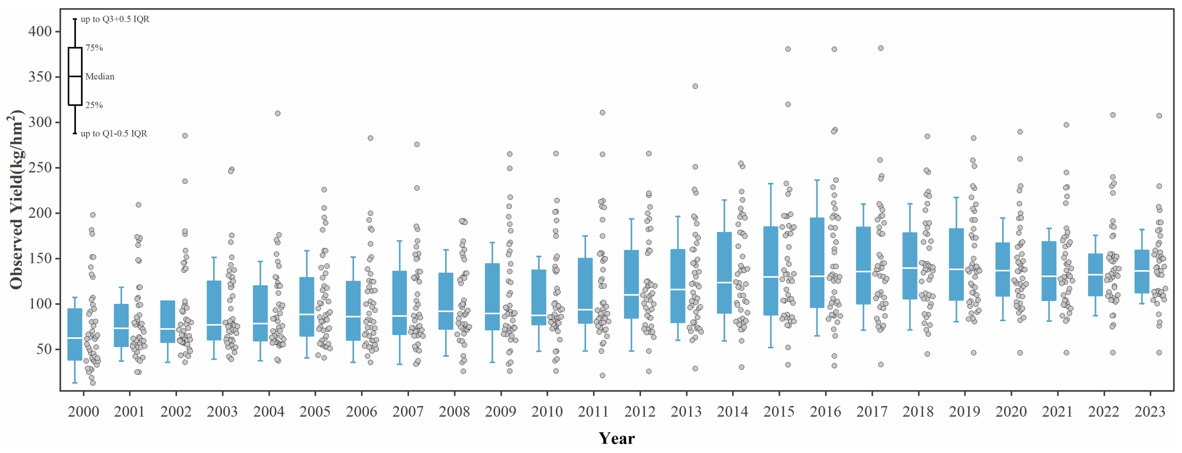
County-level data on oilseed flax production and cultivation area from 2000 to 2023 were collected from the Gansu Rural Statistical Yearbook compiled by the Gansu Provincial Rural Yearbook Editorial Committee [65,66,67,68,69,70,71,72,73,74,75,76,77,78,79,80,81,82,83,84,85,86,87,88]. Figure 2 presents a box plot illustrating the distribution of oilseed flax yields during this period. Prior to analysis, basic quality control procedures were applied to ensure data reliability. These included: (i) exclusion of counties with incomplete yield records for certain years within the study period, and (ii) removal of abnormal yield values that exceeded physiologically plausible ranges for oilseed flax, which were considered likely to result from reporting or recording errors. After quality control, the remaining yield records were used for model training and evaluation.

2.3. Methods

2.3.1. XGBoost

XGBoost (eXtreme Gradient Boosting) is an ensemble learning algorithm built upon the gradient boosting framework. It enhances model fitting accuracy by iteratively constructing multiple weak decision trees and minimizing prediction errors through gradient-based optimization [89]. During training, XGBoost incorporates regularization terms to mitigate overfitting. In addition, techniques such as column sampling, parallel computation, and automatic handling of missing values improve the model’s efficiency and robustness when processing high-dimensional and large-scale datasets. In recent years, XGBoost has been extensively applied in agricultural studies, demonstrating remarkable predictive performance in crop yield estimation. Compared with traditional algorithms such as Random Forest (RF) and Support Vector Machines (SVM), XGBoost more effectively captures nonlinear feature interactions and exhibits stronger robustness when handling multi-source heterogeneous data [90].

In this study, XGBoost was implemented as a representative traditional machine learning baseline using the scikit-learn library. The optimal hyperparameters were determined through a grid search combined with fivefold cross-validation. The final configuration was as follows: maximum tree depth of 4 and a total of 150 estimators, learning rate of 0.1, and minimum child weight of 5. To further alleviate overfitting, the subsample ratio and colsample_bytree ratio were set to 0.84 and 0.96, respectively.

2.3.2. LSTM

Long Short-Term Memory (LSTM), proposed by Hochreiter and Schmidhuber [91], is an improved variant of the traditional Recurrent Neural Network (RNN). By introducing memory cells and gating mechanisms (including the input gate, forget gate, and output gate), LSTM effectively mitigates the gradient vanishing and exploding problems commonly encountered in long-sequence modeling, thereby improving the network’s capability to capture long-term temporal dependencies. In this study, the designed LSTM model comprises two stacked LSTM layers to extract essential temporal patterns from multi-sequence inputs. The first LSTM layer contains 64 units and outputs the full sequence (return_sequences = True), while the second layer includes 32 units and provides the final temporal representation. A ReLU activation function is applied after each LSTM layer to enhance nonlinear feature learning. To reduce the risk of overfitting, a Dropout layer with a dropout rate of 0.2 is inserted after each LSTM layer. Finally, a fully connected (Dense) layer is employed to output the regression prediction of oilseed flax yield.

2.3.3. Input Feature Construction for Sequence Models

This section describes the construction of model-ready input features for sequence-based models, including the Transformer and the proposed CNN–Informer framework. These models share the same input feature definition and temporal organization. Based on the phenological characteristics of oilseed flax in Gansu Province, all dynamic variables were organized over the growing season from March to August, covering the complete crop growth cycle across counties. For each county $c$ and year $y$, remote sensing vegetation indices and climatic variables were aggregated to monthly mean values, resulting in a six-step temporal sequence. The dynamic input for each county–year sample is defined as:

$$X_{\left(c,y\right)}=\left[x_{\left(c,y,3\right)},x_{\left(c,y,4\right)},\dots ,x_{\left(c,y,8\right)}\right]\in R^{\left(T\times F\right)}$$

(3)

where $T=6$ denotes the number of monthly time steps (March–August), F represents the number of dynamic features per month, and $x_{c,y,m}$ is the feature vector for month m, formed by concatenating vegetation indices and climatic variables for the same county and year. All dynamic variables are temporally aligned at the monthly scale, such that meteorological variables and vegetation indices from the same month correspond to each other. Soil properties were treated as static features as they exhibited negligible interannual variation over the study period. Topsoil attributes (0–30 cm) were spatially averaged within each county and appended as time-invariant predictors to the model. When historical yield information was included, a yield window of length $H$ years was constructed as:

$$h_{\left(c,y\right)}=\left[Y_{\left(c,y-1\right)},Y_{\left(c,y-2\right)},\dots ,Y_{\left(c,y-H\right)}\right]$$

(4)

and fused with the learned sequence representation during model integration.

Each training sample thus corresponds to one county–year pair, with a monthly sequence of multi-source dynamic features and associated static attributes as input, and the annual county-level oilseed flax yield as the prediction target.

2.3.4. Transformer

The Transformer model has demonstrated superior performance in handling sequential data and often outperforms traditional recurrent models such as RNNs and LSTMs in capturing long-range temporal dependencies [92,93]. Its architecture is composed of stacked encoder–decoder modules that integrate multi-head self-attention and position-wise feedforward neural networks, along with residual connections and layer normalization [94]. The core operation of the self-attention mechanism can be expressed as:

$$\begin{array}{c}Attention\left(V,K,Q\right)=softmax\left({\displaystyle \frac{Q{K}^T}{\sqrt{d_K}}}\right)V\end{array}$$

(5)

where $d_K$ denotes the dimension of the key vectors; softmax represents the activation function; and Attention refers to the attention function. In this study, we constructed a two-layer Transformer encoder as a comparative model. Each encoder layer incorporated a multi-head self-attention mechanism with four attention heads and a feedforward neural network. Residual connections, layer normalization, and a Dropout layer (drop rate of 0.2) were applied after each sublayer to improve generalization stability. The feedforward network consisted of two fully connected layers, with 128 hidden units in the first layer (ReLU activation) and an output dimension matching the input embedding size in the second layer. After passing through the two encoder layers, sequence representations were aggregated via a GlobalAveragePooling1D layer, followed by Dropout (drop rate of 0.2), and finally mapped to a single regression output for oilseed flax yield prediction through a Dense layer.

2.3.5. CNN–Informer

Convolutional Neural Networks (CNNs) are a class of typical feedforward neural networks characterized by multi-layer structures and parameter-sharing mechanisms, and they have been widely adopted across deep learning applications. Their core strength lies in automatically extracting local spatial or temporal features through convolution operations and progressively constructing higher-level abstract representations. In computer vision, two-dimensional CNNs (2D-CNNs) have achieved remarkable success in image recognition, object detection, and semantic segmentation tasks [95]. However, for sequential or time-series data, one-dimensional CNNs (1D-CNNs) are more appropriate, as they effectively capture local temporal dependencies by applying convolutional kernels along the time axis. Additionally, 1D-CNNs possess advantages such as parameter efficiency, reduced computational cost, and strong parallelization capability. The convolution operation can be formally expressed as:

$$\begin{array}{c}\begin{array}{c}{y}_i=\sigma \left({\displaystyle \sum _{j=0}^{m-1}}{\omega }_j\cdot x_{i+j}+b_c\right)\end{array}\end{array}$$

(6)

where $y_i$ denotes the element at position iii in the output sequence, $\omega$ represents a convolution kernel of size $m$, and $x_{i+j}$ denotes the element of the input sequence $x$ at position $i+j$. The convolution kernel slides over the input sequence, performing element-wise multiplication and summation on the local segment at each position, followed by the addition of a bias term $b_c$. The final result is then processed by a nonlinear activation function $\sigma (·)$.

Traditional Transformer architectures suffer from significant memory and computational costs when processing long sequences due to their global attention calculations, making them difficult to apply in resource-constrained practical scenarios. To overcome this challenge, Zhou et al. [96] proposed the Informer model, which introduces a ProbSparseAttention mechanism—a sparse attention strategy that selectively computes attention only for the most informative queries. This design effectively eliminates redundant attention operations, reducing overall computational complexity from O(L²) to O(LlogL) while maintaining strong sequence modeling capabilities. Consequently, the Informer achieves substantial improvements in efficiency and scalability, making it more suitable for long-horizon time-series forecasting tasks. The core architecture of Informer consists of multi-head sparse self-attention layers, a feedforward neural network (FFN), residual connections, and layer normalization. The computation in the FFN layer can be expressed as:

$$FFN\left(x\right)=ReLU\left(x{W}_1+b_1\right)W_2+b_2$$

(7)

Here, $W_1\in {\mathbb{R}}^{d\times d_{ff}}$ and $W_2\in {\mathbb{R}}^{d_{ff}\times d}$ represent the weight matrices for the two fully connected layers, respectively, while $b_1$ and $b_2$ denote the corresponding bias terms; $d$ denotes the model dimension, and $d_{ff}$ denotes the hidden dimension of the feedforward layer. Within each Encoder Layer, the Informer stacks modules in the following sequence: first, the input is fed into the ProbSparseMulti-HeadAttention module and processed through LayerNormalization via a residual connection. Subsequently, it is passed into the FFN layer, also employing a residual structure and normalization operation, as defined by the formula:

$${\mathbf{Z}}_1=LayerNorm\left(\mathbf{X}+ProSparseMultiHead\left(\mathbf{X}\right)\right)$$

(8)

$${\mathbf{Z}}_2=LayerNorm\left({\mathbf{Z}}_1+FFN\left({\mathbf{Z}}_1\right)\right)$$

(9)

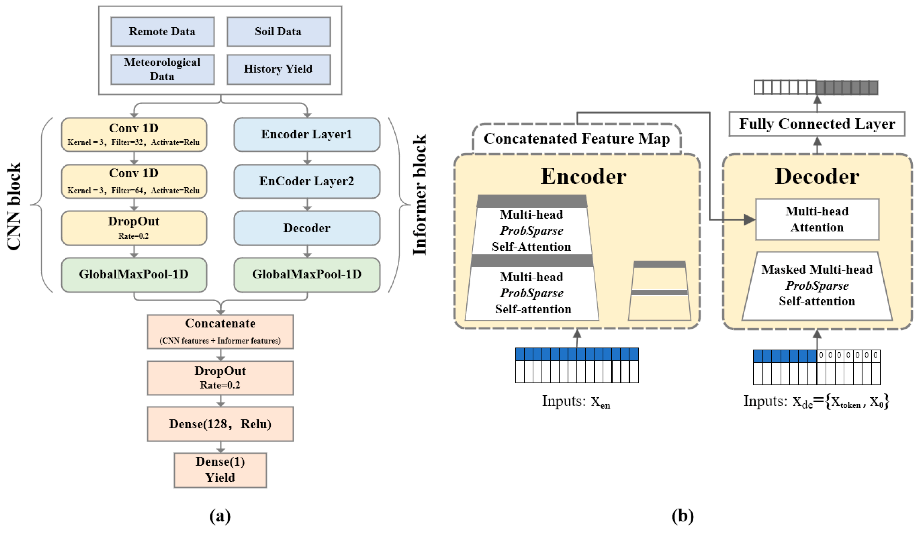
Here, $\mathbf{X}\in {\mathbb{R}}^{\mathit{L}\times \mathit{d}}$ represents the input sequence, where $L$ denotes the time step and $d$ denotes the feature dimension; ProbSparseMultiHead denotes a multi-head self-attention mechanism based on sparse attention; $FFN$ refers to a two-layer feedforward network; LayerNorm denotes a layer normalization operation; ${\mathit{Z}}_2$ denotes the output of the current encoding layer. Building upon the Informer architecture, this study integrates a convolutional neural network (CNN) with ProbSparse attention to construct a CNN–Informer hybrid model for county-level oilseed flax yield prediction using multi-source spatiotemporal data (Figure 3). The CNN branch was designed to capture local temporal patterns from multi-dimensional input sequences and consisted of two one-dimensional convolutional layers with kernel size 3, stride 1, and filter numbers of 32 and 64, respectively. ReLU activation was applied after each convolution to enhance nonlinear feature extraction. Dropout with a rate of 0.2 was introduced after each convolutional layer to mitigate overfitting. A MaxPooling1D operation was optionally applied depending on the input sequence length, followed by a GlobalMaxPooling1D layer to aggregate temporal information into a fixed-length feature representation.

The Informer component focuses on modeling long-range temporal dependencies and comprises two encoder layers and one decoder layer. Each encoder layer adopts the ProbSparse self-attention mechanism, which selects dominant query–key interactions to reduce computational complexity while preserving global dependency modeling capability. The attention module employs four attention heads and is followed by a position-wise feedforward network with a hidden dimension of 128 and ReLU activation. Residual connections, layer normalization, and dropout (rate = 0.2) are applied after both the attention and feedforward sublayers to ensure training stability. The decoder layer includes a ProbSparse self-attention module, an encoder–decoder ProbSparse cross-attention module, and a feedforward subnetwork with the same hidden dimension and regularization strategy as the encoder. The decoder output is aggregated using GlobalAveragePooling1D and concatenated with the CNN branch output for final yield prediction. The detailed architectural configuration and hyperparameter settings of the CNN–Informer model is provided in Appendix A,

Table A1. Architectural configuration and hyperparameter settings of the CNN–Informer model.

Module	Component	Hyperparameter	Value	Description
Input	Feature vector	Input feature dimension	65	Multi-source features including remote sensing, meteorological, soil, and historical yield variables
	Temporal window	Sequence length (T)	3	Historical observation window
CNN Branch	Conv1D Layer 1	Number of filters	32	Local temporal feature extraction
		Kernel size	3	Temporal receptive field
		Stride	1	Preserves temporal resolution
		Activation function	ReLU	Nonlinear transformation
	Conv1D Layer 2	Number of filters	64	Higher-level feature abstraction
		Kernel size	3	Consistent with first layer
		Stride	1	—
		Activation function	ReLU	—
	Regularization	Dropout rate	0.2	Applied after each convolutional layer
	Pooling	Strategy	GlobalMaxPooling1D	Temporal aggregation and dimensionality reduction
Informer Encoder	Encoder layers	Number of layers	2	Stacked encoder blocks
	Attention mechanism	Attention type	ProbSparse attention	Efficient long-sequences modeling
	—	Number of attention heads	4	Multi-head attention
	—	Sparsity mechanism	Top-$u$ dominant queries	Reduces redundant attention computation
	Feedforward network	$\mathrm{Hidden} \mathrm{dimension} (d_{ff}$)	128	Position-wise feedforward subnetwork
	—	Activation function	ReLU	—
	Normalization	Layer normalization	Yes	$\mathrm{Applied} \mathrm{after} \mathrm{attention} \mathrm{and} FFN$
	Regularization	Dropout rate	0.2	$\mathrm{Applied} \mathrm{to} \mathrm{attention} \mathrm{and} FFN$ modules
	Decoder layers	Number of layers	1	Single decoder block
	Self-attention	Attention type	ProbSparse attention	Decoder-side temporal modeling
	Cross-attention	Encoder–decoder attention	ProbSparse attention	Integrates encoder context
	Feedforward network	$\mathrm{Hidden} \mathrm{dimension} (d_{ff}$)	128	Same as encoder
	Regularization	Dropout rate	0.2	—
Fusion & Output	Feature fusion	Concatenation	CNN + decoder output	Multi-branch feature fusion
	Decoder aggregation	Pooling method	GlobalAveragePooling1D	Produces fixed-length decoder representation
	Output layer	Dense units	1	Yield prediction
Optimization	Optimizer	Type	Adam	Adaptive moment estimation
	Learning rate	Initial value	0.0001	Selected based on validation performance
	Loss function	Objective	Mean Squared Error (MSE)	Regression loss for yield prediction

.

2.4. Model Training and Performance Evaluation

2.4.1. Data Partitioning and Model Training

To ensure robust and fair model training, a unified training protocol was adopted by jointly considering temporal continuity, spatial independence, and consistent optimization settings. All samples were first partitioned chronologically: data from 2000 to 2018 were used for model training, data from 2019 were reserved as an independent validation set for hyperparameter tuning and early stopping, and data from 2020 to 2023 were held out for final testing. This year-based partitioning strategy effectively prevents information leakage across time and ensures that model performance reflects genuine predictive capability for future years. To further evaluate spatial generalization, a county-based spatial k-fold cross-validation strategy was employed, in which counties rather than individual samples served as the splitting units. Counties were randomly divided into five folds. In each fold, all samples from one subset of counties were excluded from training and used exclusively for validation or testing, while samples from the remaining counties were used for model training. Throughout this process, the temporal order of samples within each county was strictly preserved to maintain time-series continuity. Compared with conventional random k-fold cross-validation, this strategy enforces spatial independence and provides a more stringent assessment of model robustness in previously unseen regions. All deep learning–based models, including LSTM, Transformer, Informer, and the proposed CNN–Informer, were trained under identical optimization settings. The Adam optimizer was adopted with an initial learning rate of 0.0001, and the mean squared error (MSE) was used as the loss function. Training was conducted for a maximum of 500 epochs with a batch size of 12. To enhance training stability and mitigate overfitting, two callback mechanisms were applied consistently across all experiments: (1) EarlyStopping, which terminated training after 60 epochs without validation loss improvement and restored the best model weights, and (2) ReduceLROnPlateau, which reduced the learning rate by a factor of 0.5 after 30 epochs of stagnation, with a minimum learning rate of 1 × 10⁻⁷.

2.4.2. Evaluation Metrics for Model Performance

To comprehensively evaluate the performance and experimental results of different models, we adopted the Mean Absolute Error (MAE), Coefficient of Determination (R²), Root Mean Square Error (RMSE), and Mean Absolute Percentage Error (MAPE) as evaluation metrics. RMSE and R² are widely used evaluation metrics in crop yield prediction, with smaller RMSE values denoting greater stability and R² values nearer to 1 signifying improved accuracy and fit. We further used MAE to assess prediction accuracy, as lower values indicate superior precision. MAPE quantifies the percentage relative error against true values, offering an intuitive measure of relative prediction deviation. A joint analysis of these metrics thus enables a holistic assessment of model performance.

$$MAE={\displaystyle \frac{1}{N}}\sum _{t=1}^N\left|y_i-\widehat{y}\right|$$

(10)

$$R^2=1-{\displaystyle \frac{{\sum }_{i=1}^n{\left(y_i-{\widehat{y}}_i\right)}^2}{{\sum }_{i=1}^n{\left(y_i-\overline{y}\right)}^2}}$$

(11)

$$RMSE=\sqrt{{\displaystyle \frac{1}{n}}{\sum }_{i=1}^n{\left(y_i-{\widehat{y}}_i\right)}^2}$$

(12)

$$MAPE={\displaystyle \frac{100}{n}}\sum _{i=1}^n\left|{\displaystyle \frac{{\widehat{y}}_i-y_i}{y_i}}\right|$$

(13)

In the above equation, $n$ represents the sample size; $y_i$ and ${\widehat{y}}_i$ denote the true value and predicted value of the $i$ sample, respectively; $\overline{y}$ is the mean of the true values.

3. Results

3.1. Experiments on Historical Yield–Enhanced Time Series Modeling

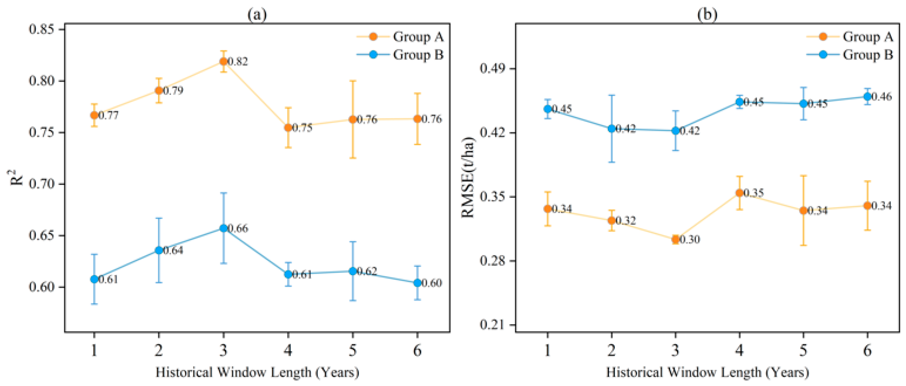
To assess the role of historical yield information in oilseed flax yield prediction, a comparative experiment was conducted between two model configurations: one incorporating historical yield features (Group A) and one excluding them (Group B). In addition, the impact of different historical window lengths (T) on model performance was systematically examined. As illustrated in Figure 4, Group A consistently outperformed Group B across all tested window lengths, with an average R² improvement ranging from approximately 11% to 17%. This result indicates that historical yield records provide valuable temporal context that cannot be fully captured by environmental variables alone. The inclusion of historical yields likely reflects the cumulative effects of management inertia, crop rotation practices, and the persistence of soil fertility conditions, all of which influence yield formation over multiple growing seasons. These legacy effects introduce temporal continuity into yield dynamics, making historical production records an informative auxiliary feature for county-level prediction. Across different window lengths, model performance exhibited a clear pattern of initial improvement followed by gradual decline as T increased. The optimal performance was observed at T = 3, corresponding to the highest mean R² (0.82) and the lowest RMSE (0.30 t/ha). At this window length, historical yield information provides sufficient temporal depth to capture medium-term yield evolution while avoiding excessive noise. The relatively small standard deviations associated with R² and RMSE at T = 3, as indicated by the error bars in Figure 4, further suggest that model performance is more consistent across repeated runs at this setting. When the historical window exceeded three years, prediction accuracy declined modestly. This decrease can be attributed to increased interannual variability in historical yields, driven by fluctuating climatic conditions and evolving management practices. Longer historical windows may introduce contextually inconsistent information and redundancy, thereby expanding the feature space and increasing the risk of overfitting, which ultimately degrades generalization performance. Based on these results, a three-year historical yield window was adopted in all subsequent experiments as a balance between informative temporal context and model complexity.

3.2. Comparative Analysis of Models Performance

3.2.1. Comparative Performance of All Models

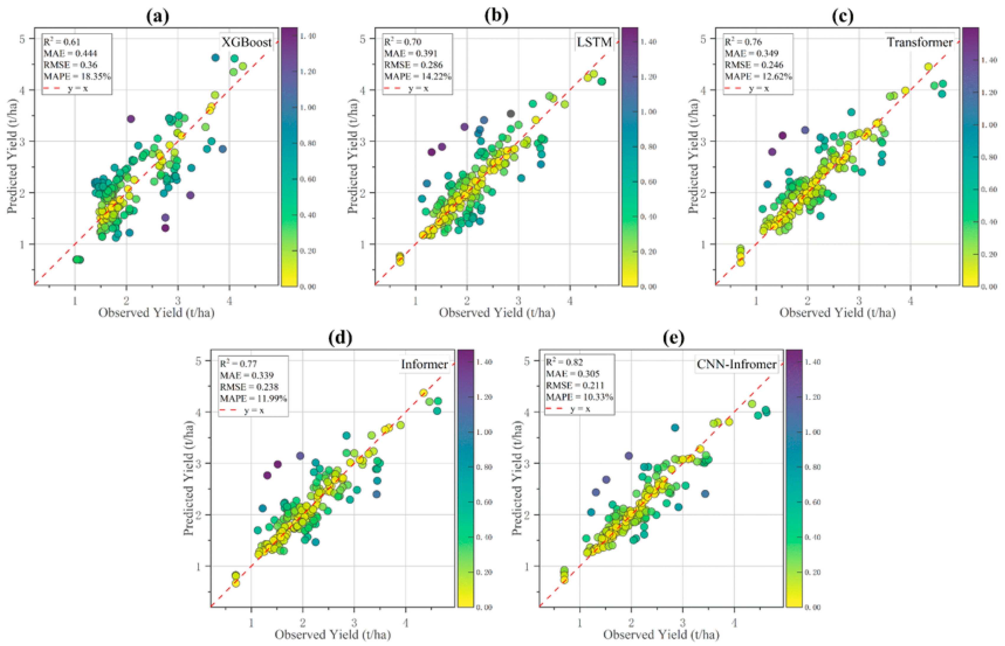
As shown in

Table 2. Performance Comparison of CNN–Informer with Other Contrastive Models.

Model	R2	RMSE (t/ha)	MAE (t/ha)	MAPE (%)
XGBoost	0.61	0.444	0.360	18.35
LSTM	0.70	0.391	0.286	14.22
Transformer	0.76	0.349	0.246	12.62
Informer	0.77	0.340	0.238	11.99
CNN–Informer	0.82	0.305	0.211	10.33

, substantial differences emerged in model performance on the full test set (2020–2023). Compared with XGBoost, all deep learning-based time-series models achieved notable improvements across evaluation metrics, with R² values exceeding 0.70, RMSE values below 0.391 t/ha, MAE values below 0.30 t/ha, and MAPE values below 15%. These results highlight the advantages of explicitly modeling temporal dependencies for oilseed flax yield prediction. Among the deep learning models, LSTM outperformed XGBoost by incorporating sequential information, while Transformer further improved performance by capturing longer-range temporal dependencies through self-attention. Informer achieved additional gains in predictive accuracy, reflecting its efficiency in modeling long time-series data and interannual variability under multi-source conditions. Notably, the proposed CNN–Informer model delivered the best overall performance, with an R² of 0.82, RMSE of 0.305 t/ha, MAE of 0.211 t/ha, and MAPE of 10.33%. These results indicate that integrating convolutional feature extraction with long-sequence temporal modeling is effective for county-level oilseed flax yield prediction.

Figure 5 presents a scatter plot depicting the relationship between the predicted and observed yields for various models on the test set (2020–2023). The figure incorporates a color-coded error band mechanism: data points are colored based on their vertical distance from the ideal 1:1 reference line (i.e., prediction error), with shades ranging from light yellow to dark, indicating increasing error magnitude. The XGBoost model exhibited relatively large dispersion and systematic bias, particularly in the mid-yield range (approximately 1.5–3.5 t/ha), indicating limited capability in capturing nonlinear relationships and temporal variability. In contrast, deep learning models showed progressively improved alignment with the 1:1 reference line, with reduced dispersion and fewer extreme deviations. Among all models, the CNN–Informer displayed the most concentrated distribution of points around the 1:1 line, with generally smaller and more evenly distributed errors across the yield range, demonstrating superior predictive consistency across counties and years.

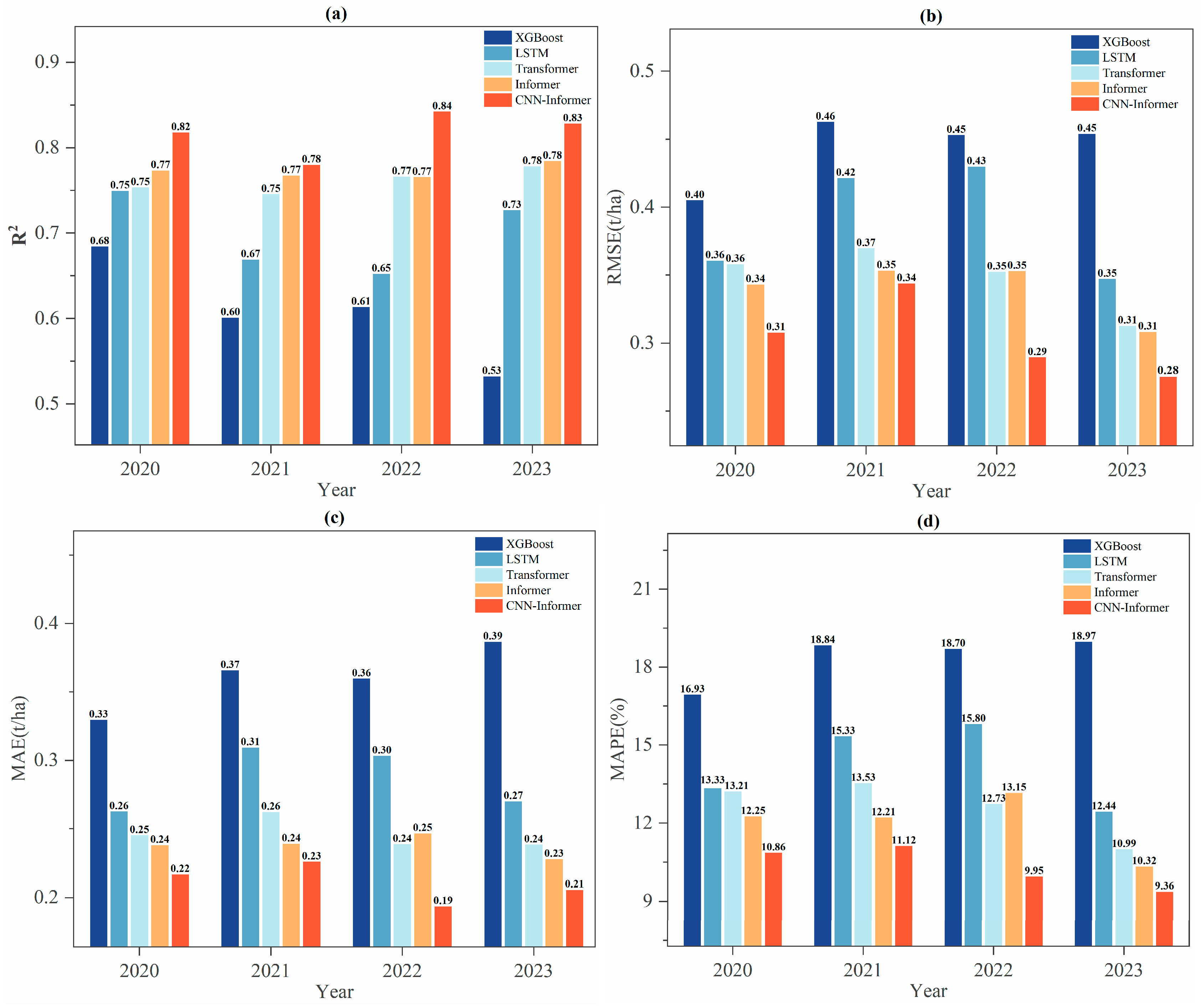
3.2.2. Performance Comparison of Models Across Test Years

Table 3. Performance comparison of CNN–informer with other oilseed flax yield prediction models (2020–2023).

Year	Model	R2	RMSE (t/ha)	MAE (t/ha)	MAPE (%)
2020	XGBoost	0.68	0.405	0.33	16.96
	LSTM	0.75	0.361	0.263	13.33
	Transformer	0.75	0.358	0.245	13.21
	Informer	0.77	0.343	0.238	12.26
	CNN–Informer	0.82	0.308	0.217	10.86
2021	XGBoost	0.60	0.463	0.366	16.93
	LSTM	0.67	0.421	0.309	15.33
	Transformer	0.75	0.369	0.262	13.53
	Informer	0.77	0.353	0.239	12.21
	CNN–Informer	0.78	0.343	0.226	11.12
2022	XGBoost	0.61	0.453	0.36	18.70
	LSTM	0.65	0.430	0.303	15.80
	Transformer	0.77	0.352	0.239	12.73
	Informer	0.77	0.353	0.247	13.15
	CNN–Informer	0.84	0.289	0.194	9.95
2023	XGBoost	0.53	0.454	0.387	18.97
	LSTM	0.73	0.347	0.271	12.44
	Transformer	0.78	0.313	0.238	10.99
	Informer	0.78	0.308	0.228	10.32
	CNN–Informer	0.83	0.275	0.205	9.36

and Figure 6 present the evaluation metrics of all models across different years. Overall, the deep learning-based time-series models consistently outperformed the XGBoost baseline across all years, demonstrating higher prediction accuracy and greater interannual stability. Among them, the proposed CNN–Informer achieved the best performance for each test year, with R² values exceeding 0.78 and reaching a maximum of 0.84 in 2022. Correspondingly, RMSE and MAE values were consistently lower than those of the other models, while MAPE remained below 11% throughout the study period and reached a minimum of 9.36% in 2023. Compared with Transformer, Informer generally exhibited lower MAE and MAPE values in multiple years, indicating improved stability in year-to-year yield prediction. The LSTM model achieved reasonable performance in earlier test years (e.g., R² = 0.75 in 2020) but showed noticeable degradation in 2022 (R² = 0.65), suggesting limited robustness under increased temporal and spatial complexity. In contrast, the XGBoost model consistently produced the lowest accuracy across all years, with R² declining to 0.53 in 2023 and relatively large prediction errors, highlighting the limitations of static learning approaches in modeling interannual yield variability. Overall, the year-by-year results demonstrate that models with stronger temporal modeling capacity exhibit more stable and accurate performance under varying climatic conditions, with CNN–Informer showing the highest robustness across different test years.

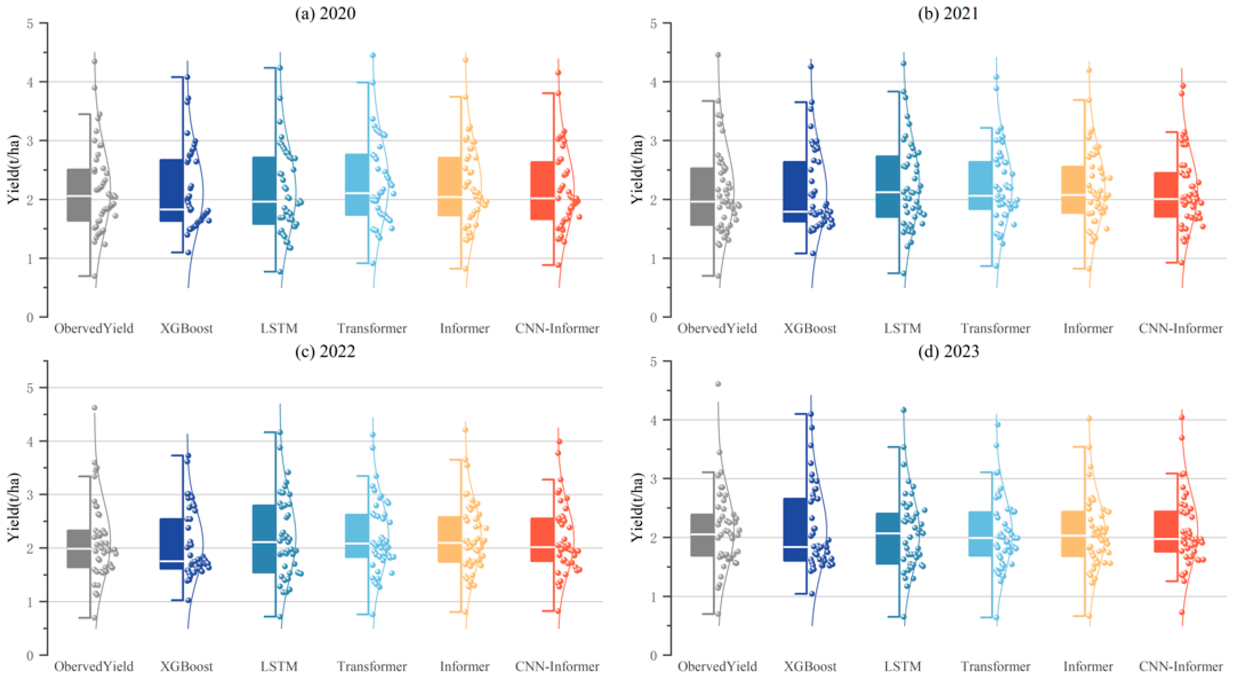
Figure 7 presents box-and-scatter plots comparing the distributions of the predicted and observed oilseed flax yields across test years. The box plots summarize the central tendency and spread of yield predictions for each model, while the overlaid scatter points illustrate the dispersion of individual samples. Overall, the CNN–Informer model produced yield distributions that more closely aligned with the observed yield ranges across all test years, with fewer extreme deviations. In contrast, the XGBoost model showed a wider spread of predicted yields and a higher frequency of samples deviating from the observed distribution. Among the deep learning models, Informer generally exhibited a more concentrated yield distribution than Transformer and LSTM, whereas LSTM shows larger dispersion in predicted yields across years. These distributional differences indicate clear performance gaps among models in representing the overall yield patterns at the county level.

3.3. Assessment of Model Performance Under Different Feature Input Configurations

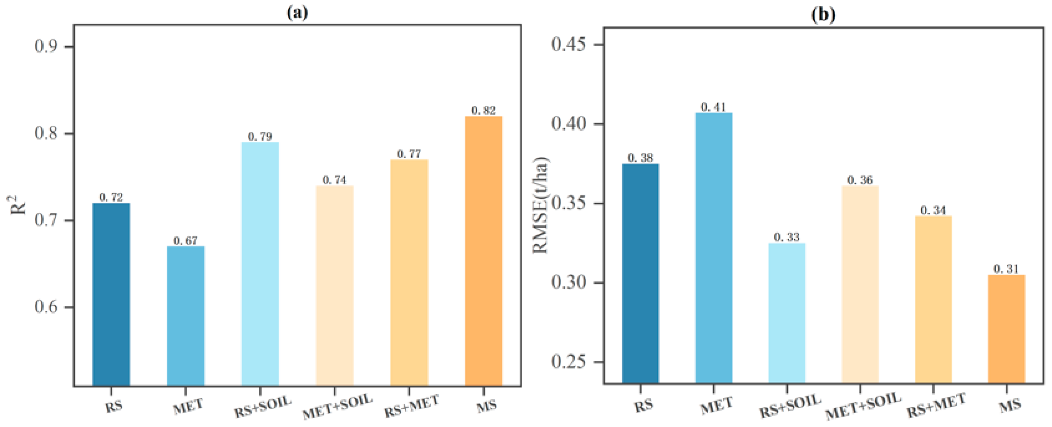
To further clarify the practical value of different data sources in oilseed flax yield prediction, we conducted a feature combination experiment by progressively integrating remote sensing, meteorological, and soil variables. The quantitative results are summarized in

Table 4. Model evaluation metrics under different data source combinations.

Combination of Data Sources	R2	RMSE (t/ha)	MAE (t/ha)	MAPE (%)
Remote sensing Data (RS)	0.72	0.375	0.260	12.78
Meteorological Data (MET)	0.67	0.407	0.291	15.51
Remote sensing Data and Soil Data (RS + SOIL)	0.79	0.325	0.229	11.38
Meteorological data and Soil Data (MET + SOIL)	0.74	0.361	0.263	13.07
Remote sensing Data and Meteorological Data (RS + MET)	0.77	0.342	0.239	12.27
Multi-Source Data (MS)	0.82	0.305	0.211	10.33

, and the relative contributions of different feature groups are further illustrated using bar charts in Figure 8 for intuitive comparison. When individual data sources were used, remote sensing features yielded the highest predictive accuracy, with an R² of 0.72, RMSE of 0.375 t/ha, and MAPE of 12.78, outperforming meteorological variables alone. Using meteorological data only resulted in lower accuracy, reflecting its more indirect relationship with yield at the county scale. Combining remote sensing and meteorological variables led to a moderate improvement in model performance compared with single-source inputs, indicating partial complementarity as well as potential information overlap between these two dynamic data sources. The inclusion of soil variables further improved model performance. Without soil information, the model achieved an R² of 0.77, RMSE of 0.342 t/ha, and MAPE of 12.27. After incorporating soil data, performance increased to an R² of 0.82, with RMSE and MAPE reduced to 0.305 t/ha and 10.33, respectively. These results suggest that soil attributes provide additional spatial context related to long-term production conditions, contributing to improved yield prediction when combined with dynamic remote sensing and meteorological features.

3.4. County-Level Five-Fold Cross-Validation Experiment

To evaluate model performance under cross-county prediction scenarios, a county-level fivefold cross-validation experiment was conducted. This experimental setting focuses on assessing how the model performs when applied to counties that are not included in the training process, providing a strict test of spatial transfer across administrative regions. Based on the feature combination experiments, two representative input configurations were selected: (1) a combination of remote sensing and meteorological variables, and (2) a multi-source configuration that additionally incorporates soil variables. A county-based fivefold cross-validation strategy was adopted, in which counties rather than individual samples served as the splitting units. In each fold, all samples from one subset of counties were excluded from training and used exclusively for testing. Specifically, data from 2018 and earlier years in 80% of the counties were used for model training, data from 2019 were used for validation, and data from 2020 to 2023 from the remaining 20% of counties were reserved for testing. In each fold, the model was reinitialized and trained independently to ensure consistency across cross-validation iterations.

The evaluation results are summarized in

Table 5. Model evaluation metrics under fivefold cross-validation.

Feature Combination	Fold	R2	RMSE (t/ha)	MAE (t/ha)	MAPE (%)
Remote sensing and Meteorological data	Fold 1	0.65	0.232	0.187	9.51
	Fold 2	0.61	0.452	0.307	13.85
	Fold 3	0.88	0.275	0.224	12.93
	Fold 4	0.65	0.493	0.352	12.83
	Fold 5	0.70	0.296	0.247	13.60
	Average	0.70	0.350	0.263	12.54
Multi-Source data	Fold 1	0.51	0.411	0.309	15.06
	Fold 2	0.58	0.407	0.323	14.58
	Fold 3	0.74	0.396	0.324	23.00
	Fold 4	0.40	0.645	0.460	17.98
	Fold 5	0.43	0.548	0.341	16.96
	Average	0.53	0.481	0.351	17.12

. When using remote sensing and meteorological variables, the model achieved an average R² of 0.70, with an RMSE of 0.350 t/ha and a MAPE of 12.54%. In comparison, the multi-source configuration yielded a lower average R² of 0.53 and a higher RMSE of 0.481 t/ha. Performance also varied more substantially across folds for the multi-source configuration, as reflected by the wider range of R² values among different county subsets. These results indicate that incorporating soil variables does not necessarily improve prediction performance when the model is applied to previously unseen counties under the current experimental setting. While soil properties provide long-term background information on regional production conditions, the soil datasets used in this study are derived from publicly available sources with relatively coarse spatial resolution. Such static representations may not fully capture intra-county heterogeneity and can introduce location-specific patterns that are less transferable across regions. In contrast, remote sensing and meteorological variables provide temporally dynamic information that directly reflects crop growth and environmental conditions, leading to more consistent performance across different county partitions. Therefore, for applications emphasizing cross-county prediction, feature combinations based on remote sensing and meteorological data appear to be more suitable, while the use of soil variables should be carefully evaluated depending on data quality and spatial resolution.

3.5. Spatial Distribution and Error Analysis of Flax Yield Prediction

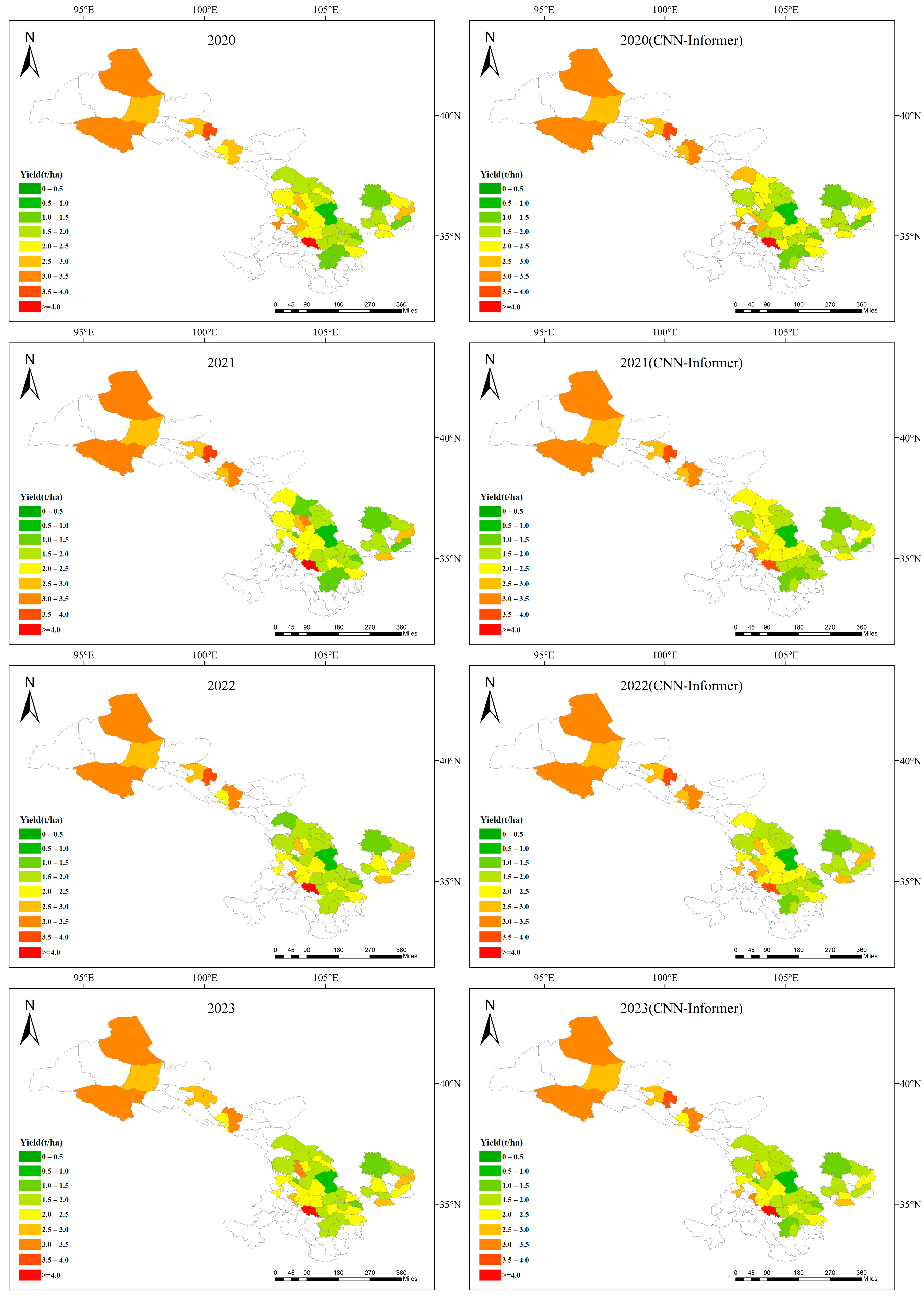
To visually depict the spatiotemporal variation in oilseed flax yield and the CNN–Informer model’s spatial predictive performance, Figure 9 shows spatial distribution maps of observed versus predicted yields for 2020–2023. The maps highlight marked regional disparities in oilseed flax distribution, with primary production concentrated in the southeast and central regions and sparser yet higher-yielding zones in the northwest. The relatively stable yield per unit area across years indicates that regional oilseed flax production systems exhibited strong resilience to interannual climatic and environmental variations. The model exhibits robust spatial generalization, accurately simulating yields in major production areas and effectively capturing inter-country yield gradients. Spatial patterns of predicted yields show a high degree of consistency with the actual distribution, particularly in central and eastern high-yield clusters, where the model successfully captures the spatial aggregation characteristics of productive areas. For instance, in 2020, the model accurately identified several high-yield counties in the northwest and central regions, while also recognizing relatively low-yield zones within the hilly southeastern areas. Similar agreement between predicted and observed spatial distributions was observed for 2021–2023, further confirming the model’s robust regional adaptability and capability in perceiving spatial yield structures.

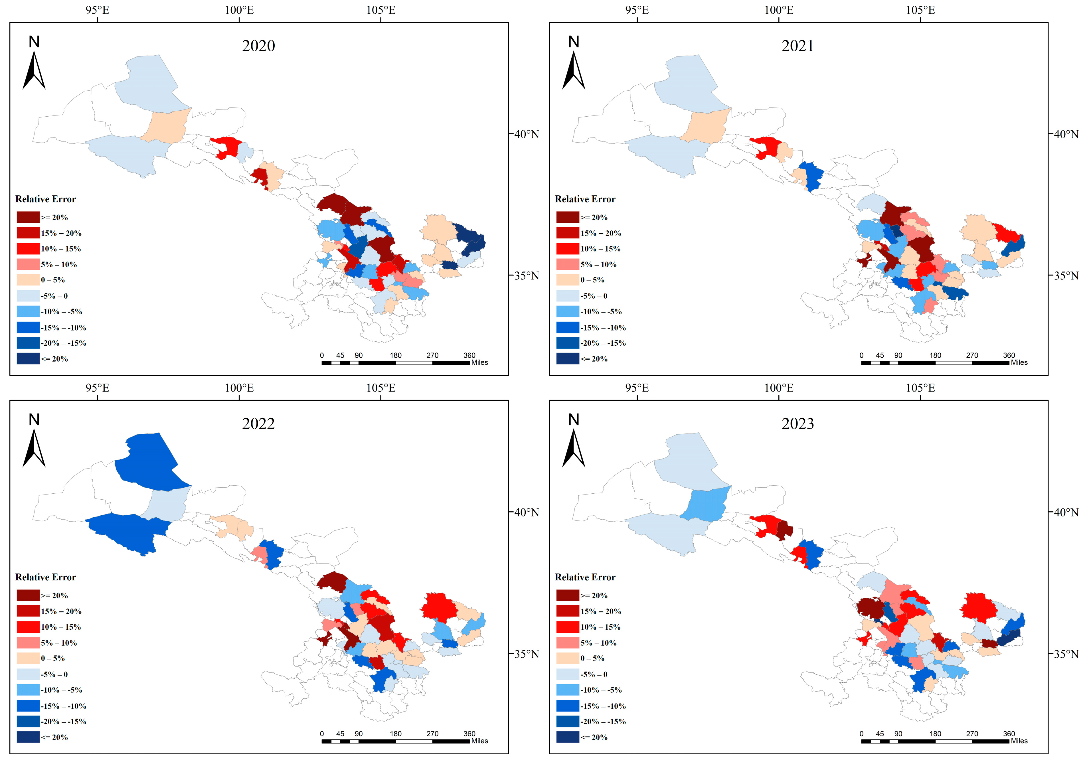
Following the spatial yield distribution analysis, Figure 9 and Figure 10 further illustrate the spatial distribution of relative errors in oilseed flax yield predictions across counties during 2000–2023. Overall, the CNN–Informer model maintained relative errors within ±10% for most counties, demonstrating strong consistency with observed yields, while only a few counties exhibited deviations exceeding ±15%. The model showed lower errors in major production areas such as central Gansu, Dingxi, and Qingyang, reflecting greater fidelity in simulating high-yield regions. Elevated errors in peripheral regions with sparse samples or pronounced climatic variations (e.g., certain counties in Hexi) may be attributed to input data quality, local meteorological disturbances, or inconsistent cultivation practices. Spatially, the model consistently showed low errors in major flax-producing areas including central Gansu (e.g., Lintao, Longxi), Dingxi City, and Qingyang. This indicates the model’s proficiency in simulating high-yield regions by effectively delineating oilseed flax yield clustering and the prominence of key production zones. This capability arises from the model’s integrated modeling of temporal dynamics and spatial patterns. However, relatively larger prediction biases were observed in several central counties, likely due to limited flax cultivation area, insufficient historical yield records, or noise in remote sensing and meteorological inputs. Furthermore, extreme local environmental conditions (e.g., high altitude, arid or windy settings) and non-standardized cultivation practices may have weakened the model’s generalization capacity. Occasional extreme meteorological events could also have amplified local prediction deviations.

4. Discussion

This study developed a CNN–Informer-based framework for county-level oilseed flax yield prediction using multi-source spatiotemporal data and evaluated its performance in terms of prediction accuracy and cross-county prediction behavior. The results revealed several consistent patterns regarding model architecture, feature contributions, and cross-regional transferability. The improved performance of the CNN–Informer model is closely related to its parallel structural design, which integrates convolutional neural networks with the Informer architecture. The CNN branch focuses on extracting localized temporal patterns, while the Informer branch captures long-range dependencies through sparse attention mechanisms. This complementary design enables the model to represent heterogeneous temporal information more effectively than sequential or single-branch architectures, providing a plausible explanation for its advantage over traditional machine learning models and other deep learning baselines in county-level yield prediction tasks.

Historical yield information was found to be an effective temporal feature. Incorporating historical yields consistently improved model performance, with a three-year window producing relatively consistent results across experiments. This finding suggests that yield formation exhibits temporal persistence at the county scale and that recent production history provides valuable contextual information for learning longer-term yield trends. Such persistence likely reflects the combined influence of regional environmental conditions and management practices that affect yield formation over multiple growing seasons. Analysis of feature contributions further revealed clear differences among data sources. Remote sensing indices consistently provided the strongest predictive signal, reflecting their ability to directly encode crop growth dynamics and interannual variability in a timely and spatially explicit manner.

Meteorological variables contributed additional environmental context but exhibited comparatively weaker predictive power, likely due to their spatial aggregation and indirect relationship with yield formation processes. As a result, combining meteorological variables with remote sensing indices resulted in only marginal performance gains, indicating partial complementarity as well as potential information overlap between these two dynamic data sources. The effect of soil variables was more complex. In global feature combination experiments, soil attributes improved the overall fitting performance by providing region-specific background information associated with baseline yield levels. However, county-level cross-validation showed that this improvement did not consistently translate into better performance when predicting yields in previously unseen counties. In some cases, models incorporating soil variables exhibited lower predictive accuracy under cross-county evaluation. This pattern suggests that the contribution of soil data may be conditional on the similarity between training and target regions. A likely explanation lies in the static nature of soil attributes and the relatively coarse spatial resolution of publicly available soil datasets. While such information can enhance model fitting within known regions, it may inadequately capture intra-county heterogeneity and local soil management differences. Consequently, soil features may introduce location-specific patterns that are difficult to transfer across counties with distinct soil characteristics. These findings indicate that the effectiveness of soil data depends not only on their relevance but also on their spatial resolution and consistency with the target prediction scale. The cross-county validation results highlight a trade-off between maximizing overall fitting accuracy and maintaining transferable performance across regions. Feature combinations dominated by dynamic variables, such as remote sensing and meteorological data, tended to show more consistent behavior across different county partitions, whereas the full multi-source configuration exhibited larger performance variation across folds. This observation suggests that feature selection should be aligned with modeling objectives, particularly when regional transferability is a primary concern. From a broader perspective, the prediction accuracy achieved by the proposed CNN–Informer model is consistent with the performance range reported in recent deep learning- and attention-based yield prediction studies. For example, Informer-based frameworks integrating time-series satellite observations and environmental variables have reported R² values on the order of 0.8 for regional rice yield prediction, demonstrating the effectiveness of sparse-attention architectures in modeling long-term temporal dependencies in agricultural systems [36]. In addition, satellite-driven yield estimation studies for major crops commonly report county- or provincial-scale accuracies in the range of R² ≈ 0.7–0.8, although the reported error magnitudes vary substantially with crop type, spatial aggregation level, and input data configuration [97]. Recent Transformer-based approaches applied to crop yield prediction further indicate that attention mechanisms outperform conventional CNN–LSTM architectures when modeling spatiotemporal satellite time series, particularly under heterogeneous agro-environmental conditions [98]. Within this context, the best performance achieved in this study (R² = 0.82, RMSE = 0.305 t/ha) fell within the expected accuracy envelope of recent attention-based approaches. Direct numerical comparisons across studies should nevertheless be interpreted with caution, given substantial differences in crop types, climatic regimes, spatial scales, and evaluation protocols. Notably, oilseed flax in Gansu Province is cultivated under more heterogeneous arid and semi-arid conditions than many staple crops examined in previous studies, posing additional challenges for robust county-level yield prediction.

Although the proposed framework achieved competitive predictive accuracy across multiple years, prediction uncertainty is likely to increase under pronounced environmental anomalies. Incorporating uncertainty-aware modeling strategies, such as ensemble learning or stochastic regularization, may help better characterize prediction uncertainty and improve result interpretability. In addition, the integration of higher-resolution soil data, phenology-related indicators, explicit spatial dependency modeling, and transfer learning techniques could further enhance model applicability across broader geographic regions. The findings highlight the need to balance feature richness with cross-regional applicability and underscore the importance of dynamic spatiotemporal information for large-scale yield prediction tasks.

5. Conclusions

This study presents and evaluates a CNN–Informer-based framework for county-level oilseed flax yield prediction using multi-source spatiotemporal data. By integrating convolutional neural networks with the Informer architecture in a parallel design, the framework effectively captures both localized temporal variations and long-range dependencies—features inherent to agricultural yield time series shaped by short-term environmental fluctuations and long-term agronomic trends. Comparative experiments demonstrate that this hybrid architecture consistently outperformed both conventional machine learning models and established deep learning baselines, underscoring its suitability for modeling heterogeneous agricultural systems at the regional scale. Feature-level analyses further showed that remote sensing indices provide the most informative signals for yield prediction due to their direct sensitivity to crop growth dynamics throughout the growing season, while meteorological variables mainly supply complementary environmental context. Historical yield information enhances the model’s ability to learn temporal persistence in yield formation, with a three-year historical window yielding the most stable performance, indicating that recent production history provides valuable contextual information for modeling long-term yield trends. In contrast, soil variables act primarily as region-specific background features that improve in-sample fitting. However, their utility for spatial generalization is limited: because publicly available soil datasets are static and coarse-resolution, they often encode location-specific patterns that fail to generalize to unseen counties. County-level cross-validation revealed a clear trade-off between optimizing in-sample accuracy and ensuring robust out-of-sample generalization. Notably, feature sets dominated by dynamic variables—such as remote sensing and meteorological data—exhibited markedly more stable performance under regional transfer scenarios. These findings point to several promising directions for future work. First, refining the temporal granularity of input features—for instance, by partitioning the growing season into ten-day or weekly intervals—could better resolve critical phenological stages and facilitate earlier yield forecasting. Second, explicitly modeling spatial interactions among counties via graph neural networks or spatially aware Transformer architectures may further improve regional generalization. Finally, applying the framework to other oilseed flax-producing regions or adjacent provinces through transfer learning would offer a rigorous test of its adaptability across diverse agro-environmental settings. Overall, the CNN–Informer framework offers an effective approach for county-level oilseed flax yield prediction in arid and semi-arid regions. The findings highlight the need to balance feature richness with cross-regional applicability and underscore the importance of dynamic spatiotemporal information for large-scale yield prediction tasks.

References

1. Kavita, M.; Mathur, P. Crop yield estimation in India using machine learning. In Proceedings of the 2020 IEEE 5th International Conference on Computing Communication and Automation (ICCCA), Greater Noida, India, 30–31 October 2020; pp. 220–224. [Google Scholar]
2. Diederichsen, A.; Fu, Y.B. Flax genetic diversity as the raw material for future success. In Proceedings of the International Conference on Flax and Bast Plants, Saskatoon, SK, Canada, 21–23 July 2008; pp. 270–280. [Google Scholar]
3. FAOSTAT. FAOSTAT Database; Food and Agriculture Organization: Rome, Italy, 2023. [Google Scholar]
4. Ibrar, D.; Ahmad, R.; Mirza, M.; Mahmood, T.; Khan, M.; Iqbal, M.S. Correlation and path analysis for yield and yield components in linseed (Linum usitatissimum L.). J. Agric. Res. 2016, 54, 153–159. [Google Scholar]
5. Harvey, M.L. Evaluation of the Performance of the Western Canadian Flaxseed Marketing System. Master’s Thesis, University of Saskatchewan, Saskatoon, SK, Canada, 1993. [Google Scholar]
6. Payasi, D.K.; Garg, D.; Payasi, S.; Yogranjan. Chapter 2.1—Preharvesting processing of linseed crop. In Linseed; Langyan, S., Kumar, A., Eds.; Academic Press: Cambridge, MA, USA, 2024; pp. 21–45. [Google Scholar]
7. Madhukar, A.; Kumar, V.; Dashora, K. Temperature and precipitation are adversely affecting wheat yield in India. J. Water Clim. Change 2022, 13, 1631–1656. [Google Scholar] [CrossRef]
8. Warrick, A.W.; Gardner, W.R. Crop yield as affected by spatial variations of soil and irrigation. Water Resour. Res. 1983, 19, 181–186. [Google Scholar] [CrossRef]
9. Maitah, M.; Malec, K.; Maitah, K. Influence of precipitation and temperature on maize production in the Czech Republic from 2002 to 2019. Sci. Rep. 2021, 11, 10467. [Google Scholar] [CrossRef]
10. Huang, T.; Döring, T.F.; Zhao, X.; Weiner, J.; Dang, P.; Zhang, M.; Zhang, M.; Siddique, K.H.M.; Schmid, B.; Qin, X. Cultivar mixtures increase crop yields and temporal yield stability globally. A meta-analysis. Agron. Sustain. Dev. 2024, 44, 28. [Google Scholar] [CrossRef]
11. Laidig, F.; Feike, T.; Klocke, B.; Macholdt, J.; Miedaner, T.; Rentel, D.; Piepho, H.P. Yield reduction due to diseases and lodging and impact of input intensity on yield in variety trials in five cereal crops. Euphytica 2022, 218, 150. [Google Scholar] [CrossRef]
12. Araya, A.; Prasad, P.V.V.; Ciampitti, I.A.; Jha, P.K. Using crop simulation model to evaluate influence of water management practices and multiple cropping systems on crop yields: A case study for Ethiopian highlands. Field Crops Res. 2021, 260, 108004. [Google Scholar] [CrossRef]
13. Ye, Z.; Zhai, X.; She, T.; Liu, X.; Hong, Y.; Wang, L.; Zhang, L.; Wang, Q. Winter Wheat Yield Prediction Based on the ASTGNN Model Coupled with Multi-Source Data. Agronomy 2024, 14, 2262. [Google Scholar] [CrossRef]
14. Becker-Reshef, I.; Vermote, E.; Lindeman, M.; Justice, C. A generalized regression-based model for forecasting winter wheat yields in Kansas and Ukraine using MODIS data. Remote Sens. Environ. 2010, 114, 1312–1323. [Google Scholar] [CrossRef]
15. Franch, B.; Vermote, E.F.; Becker-Reshef, I.; Claverie, M.; Huang, J.; Zhang, J.; Justice, C.; Sobrino, J.A. Improving the timeliness of winter wheat production forecast in the United States of America, Ukraine and China using MODIS data and NCAR Growing Degree Day information. Remote Sens. Environ. 2015, 161, 131–148. [Google Scholar] [CrossRef]
16. Yu, W.; Yang, G.; Li, D.; Zheng, H.; Yao, X.; Zhu, Y.; Cao, W.; Qiu, L.; Cheng, T. Improved prediction of rice yield at field and county levels by synergistic use of SAR, optical and meteorological data. Agric. For. Meteorol. 2023, 342, 109729. [Google Scholar] [CrossRef]
17. Zhuang, H.; Zhang, Z.; Cheng, F.; Han, J.; Luo, Y.; Zhang, L.; Cao, J.; Zhang, J.; He, B.; Xu, J.; et al. Integrating data assimilation, crop model, and machine learning for winter wheat yield forecasting in the North China Plain. Agric. For. Meteorol. 2024, 347, 109909. [Google Scholar] [CrossRef]
18. Feng, P.; Wang, B.; Liu, D.L.; Waters, C.; Yu, Q. Incorporating machine learning with biophysical model can improve the evaluation of climate extremes impacts on wheat yield in south-eastern Australia. Agric. For. Meteorol. 2019, 275, 100–113. [Google Scholar] [CrossRef]
19. Guan, K.; Sultan, B.; Biasutti, M.; Baron, C.; Lobell, D.B. Assessing climate adaptation options and uncertainties for cereal systems in West Africa. Agric. For. Meteorol. 2017, 232, 291–305. [Google Scholar] [CrossRef]
20. Kang, Y.; Özdoğan, M. Field-level crop yield mapping with Landsat using a hierarchical data assimilation approach. Remote Sens. Environ. 2019, 228, 144–163. [Google Scholar] [CrossRef]
21. Folberth, C.; Skalský, R.; Moltchanova, E.; Balkovič, J.; Azevedo, L.B.; Obersteiner, M.; van der Velde, M. Uncertainty in soil data can outweigh climate impact signals in global crop yield simulations. Nat. Commun. 2016, 7, 11872. [Google Scholar] [CrossRef] [PubMed]
22. Huang, J.; Tian, L.; Liang, S.; Ma, H.; Becker-Reshef, I.; Huang, Y.; Su, W.; Zhang, X.; Zhu, D.; Wu, W. Improving winter wheat yield estimation by assimilation of the leaf area index from Landsat TM and MODIS data into the WOFOST model. Agric. For. Meteorol. 2015, 204, 106–121. [Google Scholar] [CrossRef]
23. Lobell, D.B.; Thau, D.; Seifert, C.; Engle, E.; Little, B. A scalable satellite-based crop yield mapper. Remote Sens. Environ. 2015, 164, 324–333. [Google Scholar] [CrossRef]
24. Li, Y.; Guan, K.; Yu, A.; Peng, B.; Zhao, L.; Li, B.; Peng, J. Toward building a transparent statistical model for improving crop yield prediction: Modeling rainfed corn in the U.S. Field Crops Res. 2019, 234, 55–65. [Google Scholar] [CrossRef]
25. Blanc, É. Statistical emulators of maize, rice, soybean and wheat yields from global gridded crop models. Agric. For. Meteorol. 2017, 236, 145–161. [Google Scholar] [CrossRef]
26. Basso, B.; Cammarano, D.; Carfagna, E. Review of Crop Yield Forecasting Methods and Early Warning Systems. In Proceedings of the First Meeting of the Scientific Advisory Committee of the Global Strategy to Improve Agricultural and Rural Statistics, Rome, Italy, 18–19 July 2013. [Google Scholar]
27. Jeong, J.H.; Resop, J.P.; Mueller, N.D.; Fleisher, D.H.; Yun, K.; Butler, E.E.; Timlin, D.J.; Shim, K.-M.; Gerber, J.S.; Reddy, V.R.; et al. Random Forests for Global and Regional Crop Yield Predictions. PLoS ONE 2016, 11, e0156571. [Google Scholar] [CrossRef] [PubMed]
28. Khan, S.N.; Li, D.; Maimaitijiang, M. Using gross primary production data and deep transfer learning for crop yield prediction in the US Corn Belt. Int. J. Appl. Earth Obs. Geoinf. 2024, 131, 103965. [Google Scholar] [CrossRef]
29. Kuradusenge, M.; Hitimana, E.; Hanyurwimfura, D.; Rukundo, P.; Mtonga, K.; Mukasine, A.; Uwitonze, C.; Ngabonziza, J.; Uwamahoro, A. Crop Yield Prediction Using Machine Learning Models: Case of Irish Potato and Maize. Agriculture 2023, 13, 225. [Google Scholar] [CrossRef]
30. Kundu, N.; Rani, G.; Dhaka, V.S.; Gupta, K.; Nayaka, S.C.; Vocaturo, E.; Zumpano, E. Disease detection, severity prediction, and crop loss estimation in MaizeCrop using deep learning. Artif. Intell. Agric. 2022, 6, 276–291. [Google Scholar] [CrossRef]
31. Wang, J.; Wang, P.; Tian, H.; Tansey, K.; Liu, J.; Quan, W. A deep learning framework combining CNN and GRU for improving wheat yield estimates using time series remotely sensed multi-variables. Comput. Electron. Agric. 2023, 206, 107705. [Google Scholar] [CrossRef]
32. Gavahi, K.; Abbaszadeh, P.; Moradkhani, H. DeepYield: A combined convolutional neural network with long short-term memory for crop yield forecasting. Expert Syst. Appl. 2021, 184, 115511. [Google Scholar] [CrossRef]
33. Zhou, S.; Xu, L.; Chen, N. Rice Yield Prediction in Hubei Province Based on Deep Learning and the Effect of Spatial Heterogeneity. Remote Sens. 2023, 15, 1361. [Google Scholar] [CrossRef]
34. Joshi, A.; Pradhan, B.; Gite, S.; Chakraborty, S. Remote-Sensing Data and Deep-Learning Techniques in Crop Mapping and Yield Prediction: A Systematic Review. Remote Sens. 2023, 15, 2014. [Google Scholar] [CrossRef]
35. Satir, O.; Berberoglu, S. Crop yield prediction under soil salinity using satellite derived vegetation indices. Field Crops Res. 2016, 192, 134–143. [Google Scholar] [CrossRef]
36. Liu, Y.; Wang, S.; Chen, J.; Chen, B.; Wang, X.; Hao, D.; Sun, L. Rice Yield Prediction and Model Interpretation Based on Satellite and Climatic Indicators Using a Transformer Method. Remote Sens. 2022, 14, 5045. [Google Scholar] [CrossRef]
37. Saeed, U.; Dempewolf, J.; Becker-Reshef, I.; Khan, A.; Ahmad, A.; Wajid, S.A. Forecasting wheat yield from weather data and MODIS NDVI using Random Forests for Punjab province, Pakistan. Int. J. Remote Sens. 2017, 38, 4831–4854. [Google Scholar] [CrossRef]
38. Lu, J.; Li, J.; Fu, H.; Zou, W.; Kang, J.; Yu, H.; Lin, X. Estimation of rice yield using multi-source remote sensing data combined with crop growth model and deep learning algorithm. Agric. For. Meteorol. 2025, 370, 110600. [Google Scholar] [CrossRef]
39. Li, M.; Wang, P.; Tansey, K.; Zhang, Y.; Guo, F.; Liu, J.; Li, H. An interpretable wheat yield estimation model using an attention mechanism-based deep learning framework with multiple remotely sensed variables. Int. J. Appl. Earth Obs. Geoinf. 2025, 140, 104579. [Google Scholar] [CrossRef]
40. Lin, F.; Crawford, S.; Guillot, K.; Zhang, Y.; Chen, Y.; Yuan, X.; Chen, L.; Williams, S.; Minvielle, R.; Xiao, X. Mmst-vit: Climate change-aware crop yield prediction via multi-modal spatial-temporal vision transformer. In Proceedings of the IEEE/CVF International Conference on Computer Vision, Paris, France, 2–3 October 2023; pp. 5774–5784. [Google Scholar]
41. Jácome Galarza, L.; Realpe, M.; Viñán-Ludeña, M.S.; Calderón, M.F.; Jaramillo, S. AgriTransformer: A Transformer-Based Model with Attention Mechanisms for Enhanced Multimodal Crop Yield Prediction. Electronics 2025, 14, 2466. [Google Scholar] [CrossRef]
42. Raza, A.; Shahid, M.A.; Zaman, M.; Miao, Y.; Huang, Y.; Safdar, M.; Maqbool, S.; Muhammad, N.E. Improving Wheat Yield Prediction with Multi-Source Remote Sensing Data and Machine Learning in Arid Regions. Remote Sens. 2025, 17, 774. [Google Scholar] [CrossRef]
43. Huang, J.; Wang, X.; Li, X.; Tian, H.; Pan, Z. Remotely Sensed Rice Yield Prediction Using Multi-Temporal NDVI Data Derived from NOAA’s-AVHRR. PLoS ONE 2013, 8, e70816. [Google Scholar] [CrossRef] [PubMed]
44. Clarke, A.; Yates, D.; Blanchard, C.; Islam, M.Z.; Ford, R.; Rehman, S.-U.; Walsh, R.P. Integrating Climate and Satellite Data for Multi-Temporal Pre-Harvest Prediction of Head Rice Yield in Australia. Remote Sens. 2024, 16, 1815. [Google Scholar] [CrossRef]
45. Gao, Y. Oilseed flax (Linum usitatissimum L.), an emerging functional cash crop of China. Oil Crop Sci. 2020, 5, 23. [Google Scholar] [CrossRef]
46. Wang, S.; Zhang, Q.; Wang, J.; Liu, Y.; Zhang, Y. Relationship between Drought and Precipitation Heterogeneity: An Analysis across Rain-Fed Agricultural Regions in Eastern Gansu, China. Atmosphere 2021, 12, 1274. [Google Scholar] [CrossRef]
47. An, D.; Du, Y.; Berndtsson, R.; Niu, Z.; Zhang, L.; Yuan, F. Evidence of climate shift for temperature and precipitation extremes across Gansu Province in China. Theor. Appl. Climatol. 2020, 139, 1137–1149. [Google Scholar] [CrossRef]
48. Zeng, Z.; Wu, W.; Li, Z.; Zhou, Y.; Huang, H. Quantitative Assessment of Agricultural Drought Risk in Southeast Gansu Province, Northwest China. Sustainability 2019, 11, 5533. [Google Scholar] [CrossRef]
49. Li, Q.; Yang, J.; Guan, W.; Liu, Z.; He, G.; Zhang, D.; Liu, X. Soil fertility evaluation and spatial distribution of grasslands in Qilian Mountains Nature Reserve of eastern Qinghai-Tibetan Plateau. PeerJ 2021, 9, e10986. [Google Scholar] [CrossRef]
50. Manns, H.R.; Parkin, G.W.; Martin, R.C. Evidence of a union between organic carbon and water content in soil. Can. J. Soil. Sci. 2016, 96, 305–316. [Google Scholar] [CrossRef]
51. Becker-Reshef, I.; Justice, C.; Sullivan, M.; Vermote, E.; Tucker, C.; Anyamba, A.; Small, J.; Pak, E.; Masuoka, E.; Schmaltz, J.; et al. Monitoring Global Croplands with Coarse Resolution Earth Observations: The Global Agriculture Monitoring (GLAM) Project. Remote Sens. 2010, 2, 1589–1609. [Google Scholar] [CrossRef]
52. Yuan, W.; Zheng, Y.; Piao, S.; Ciais, P.; Lombardozzi, D.; Wang, Y.; Ryu, Y.; Chen, G.; Dong, W.; Hu, Z.; et al. Increased atmospheric vapor pressure deficit reduces global vegetation growth. Sci. Adv. 2019, 5, eaax1396. [Google Scholar] [CrossRef]
53. Abatzoglou, J.T. TerraClimate: Monthly Climate and Climatic Water Balance for Global Terrestrial Surfaces; University of California Merced: Merced, CA, USA, 2024. [Google Scholar]
54. Cihlar, J.; St Laurent, L.; Dyer, J.A. Relation between the normalized difference vegetation index and ecological variables. Remote Sens. Environ. 1991, 35, 279–298. [Google Scholar] [CrossRef]
55. Wang, Q.; Moreno-Martínez, Á.; Muñoz-Marí, J.; Campos-Taberner, M.; Camps-Valls, G. Estimation of vegetation traits with kernel NDVI. ISPRS J. Photogramm. Remote Sens. 2023, 195, 408–417. [Google Scholar] [CrossRef]
56. Son, N.T.; Chen, C.F.; Chen, C.R.; Minh, V.Q.; Trung, N.H. A comparative analysis of multitemporal MODIS EVI and NDVI data for large-scale rice yield estimation. Agric. For. Meteorol. 2014, 197, 52–64. [Google Scholar] [CrossRef]
57. Huete, A.R. A soil-adjusted vegetation index (SAVI). Remote Sens. Environ. 1988, 25, 295–309. [Google Scholar] [CrossRef]
58. Jordan, C.F. Derivation of Leaf-Area Index from Quality of Light on the Forest Floor. Ecology 1969, 50, 663–666. [Google Scholar] [CrossRef]
59. Roy, B. Optimum machine learning algorithm selection for forecasting vegetation indices: MODIS NDVI & EVI. Remote Sens. Appl. Soc. Environ. 2021, 23, 100582. [Google Scholar] [CrossRef]
60. Wang, X.; Biederman, J.A.; Knowles, J.F.; Scott, R.L.; Turner, A.J.; Dannenberg, M.P.; Köhler, P.; Frankenberg, C.; Litvak, M.E.; Flerchinger, G.N.; et al. Satellite solar-induced chlorophyll fluorescence and near-infrared reflectance capture complementary aspects of dryland vegetation productivity dynamics. Remote Sens. Environ. 2022, 270, 112858. [Google Scholar] [CrossRef]
61. Cheng, M.; Jiao, X.; Jin, X.; Li, B.; Liu, K.; Shi, L. Satellite time series data reveal interannual and seasonal spatiotemporal evapotranspiration patterns in China in response to effect factors. Agric. Water Manag. 2021, 255, 107046. [Google Scholar] [CrossRef]
62. Khanal, S.; Fulton, J.; Klopfenstein, A.; Douridas, N.; Shearer, S. Integration of high resolution remotely sensed data and machine learning techniques for spatial prediction of soil properties and corn yield. Comput. Electron. Agric. 2018, 153, 213–225. [Google Scholar] [CrossRef]
63. Fischer, G.; Nachtergaele, F.O.; Prieler, S.; van Velthuizen, H.; Verelst, L.; Wiberg, D. Global Agro-Ecological Zones (GAEZ v3.0): Global Soil Data for Use in Agro-Ecological Assessments; Food and Agriculture Organization of the United Nations (FAO): Rome, Italy; International Institute for Applied Systems Analysis (IIASA): Laxenburg, Austria, 2012. [Google Scholar]
64. FAO. Harmonized World Soil Database V 1.2; FAO: Rome, Italy, 2019. [Google Scholar]
65. Gansu Provincial Rural Yearbook Editorial Committee. Gansu Rural Statistical Yearbook; China Statistics Press: Beijing, China, 2000. [Google Scholar]
66. Gansu Provincial Rural Yearbook Editorial Committee. Gansu Rural Statistical Yearbook; China Statistics Press: Beijing, China, 2001. [Google Scholar]
67. Gansu Provincial Rural Yearbook Editorial Committee. Gansu Rural Statistical Yearbook; China Statistics Press: Beijing, China, 2002. [Google Scholar]
68. Gansu Provincial Rural Yearbook Editorial Committee. Gansu Rural Statistical Yearbook; China Statistics Press: Beijing, China, 2003. [Google Scholar]
69. Gansu Provincial Rural Yearbook Editorial Committee. Gansu Rural Statistical Yearbook; China Statistics Press: Beijing, China, 2004. [Google Scholar]
70. Gansu Provincial Rural Yearbook Editorial Committee. Gansu Rural Statistical Yearbook; China Statistics Press: Beijing, China, 2005. [Google Scholar]
71. Gansu Provincial Rural Yearbook Editorial Committee. Gansu Rural Statistical Yearbook; China Statistics Press: Beijing, China, 2006. [Google Scholar]
72. Gansu Provincial Rural Yearbook Editorial Committee. Gansu Rural Statistical Yearbook; China Statistics Press: Beijing, China, 2007. [Google Scholar]
73. Gansu Provincial Rural Yearbook Editorial Committee. Gansu Rural Statistical Yearbook; China Statistics Press: Beijing, China, 2008. [Google Scholar]
74. Gansu Provincial Rural Yearbook Editorial Committee. Gansu Rural Statistical Yearbook; China Statistics Press: Beijing, China, 2009. [Google Scholar]
75. Gansu Provincial Rural Yearbook Editorial Committee. Gansu Rural Statistical Yearbook; China Statistics Press: Beijing, China, 2010. [Google Scholar]
76. Gansu Provincial Rural Yearbook Editorial Committee. Gansu Rural Statistical Yearbook; China Statistics Press: Beijing, China, 2011. [Google Scholar]
77. Gansu Provincial Rural Yearbook Editorial Committee. Gansu Rural Statistical Yearbook; China Statistics Press: Beijing, China, 2012. [Google Scholar]
78. Gansu Provincial Rural Yearbook Editorial Committee. Gansu Rural Statistical Yearbook; China Statistics Press: Beijing, China, 2013. [Google Scholar]
79. Gansu Provincial Rural Yearbook Editorial Committee. Gansu Rural Statistical Yearbook; China Statistics Press: Beijing, China, 2014. [Google Scholar]
80. Gansu Provincial Rural Yearbook Editorial Committee. Gansu Rural Statistical Yearbook; China Statistics Press: Beijing, China, 2015. [Google Scholar]
81. Gansu Provincial Rural Yearbook Editorial Committee. Gansu Rural Statistical Yearbook; China Statistics Press: Beijing, China, 2016. [Google Scholar]
82. Gansu Provincial Rural Yearbook Editorial Committee. Gansu Rural Statistical Yearbook; China Statistics Press: Beijing, China, 2017. [Google Scholar]
83. Gansu Provincial Rural Yearbook Editorial Committee. Gansu Rural Statistical Yearbook; China Statistics Press: Beijing, China, 2018. [Google Scholar]
84. Gansu Provincial Rural Yearbook Editorial Committee. Gansu Rural Statistical Yearbook; China Statistics Press: Beijing, China, 2019. [Google Scholar]
85. Gansu Provincial Rural Yearbook Editorial Committee. Gansu Rural Statistical Yearbook; China Statistics Press: Beijing, China, 2020. [Google Scholar]
86. Gansu Provincial Rural Yearbook Editorial Committee. Gansu Rural Statistical Yearbook; China Statistics Press: Beijing, China, 2021. [Google Scholar]
87. Gansu Provincial Rural Yearbook Editorial Committee. Gansu Rural Statistical Yearbook; China Statistics Press: Beijing, China, 2022. [Google Scholar]
88. Gansu Provincial Rural Yearbook Editorial Committee. Gansu Rural Statistical Yearbook; China Statistics Press: Beijing, China, 2023. [Google Scholar]
89. Chen, T.; Guestrin, C. XGBoost: A Scalable Tree Boosting System. In Proceedings of the 22nd ACM SIGKDD International Conference on Knowledge Discovery and Data Mining, San Francisco, CA, USA, 13–17 August 2016. [Google Scholar]
90. Patil, Y.; Ramachandran, H.; Sundararajan, S.; Srideviponmalar, P. Comparative Analysis of Machine Learning Models for Crop Yield Prediction Across Multiple Crop Types. SN Comput. Sci. 2025, 6, 64. [Google Scholar] [CrossRef]
91. Hochreiter, S.; Schmidhuber, J. Long Short-Term Memory. Neural Comput. 1997, 9, 1735–1780. [Google Scholar] [CrossRef]
92. Santos, R.P.d.; Matos-Carvalho, J.P.; Leithardt, V.R.Q. Deep learning in time series forecasting with transformer models and RNNs. PeerJ Comput. Sci. 2025, 11, e3001. [Google Scholar] [CrossRef] [PubMed]
93. Su, L.; Zuo, X.; Li, R.; Wang, X.; Zhao, H.; Huang, B. A systematic review for transformer-based long-term series forecasting. Artif. Intell. Rev. 2025, 58, 80. [Google Scholar] [CrossRef]
94. Vaswani, A.; Shazeer, N.M.; Parmar, N.; Uszkoreit, J.; Jones, L.; Gomez, A.N.; Kaiser, L.; Polosukhin, I. Attention is All you Need. In Proceedings of the Neural Information Processing Systems, Long Beach, CA, USA, 4–9 December 2017. [Google Scholar]
95. Krizhevsky, A.; Sutskever, I.; Hinton, G.E. ImageNet classification with deep convolutional neural networks. Commun. ACM 2017, 60, 84–90. [Google Scholar] [CrossRef]
96. Zhou, H.; Zhang, S.; Peng, J.; Zhang, S.; Li, J.; Xiong, H.; Zhang, W. Informer: Beyond Efficient Transformer for Long Sequence Time-Series Forecasting. Proc. AAAI Conf. Artif. Intell. 2020, 35, 11106–11115. [Google Scholar] [CrossRef]
97. Xie, Y.; Huang, J. Integration of a Crop Growth Model and Deep Learning Methods to Improve Satellite-Based Yield Estimation of Winter Wheat in Henan Province, China. Remote Sens. 2021, 13, 4372. [Google Scholar] [CrossRef]
98. Bi, L.; Wally, O.; Hu, G.; Tenuta, A.U.; Kandel, Y.R.; Mueller, D.S. A transformer-based approach for early prediction of soybean yield using time-series images. Front. Plant Sci. 2023, 14, 1173036. [Google Scholar] [CrossRef] [PubMed]
Figure 1. Study area of Gansu Province.
Remotesensing 18 00181 g001
Figure 2. The temporal distribution of county-level flax yield from 2000 to 2023. The box represents the interquartile range (25th–75th percentiles), with whiskers extending to Q3 + 0.5 × IQR and Q1 − 0.5 × IQR, while scatter points indicate individual yield observations for each year.
Remotesensing 18 00181 g002
Figure 3. (a) The network architecture of the CNN–Informer model for oilseed flax yield prediction. (b) The architecture of the Informer model. Squares represent different model components, arrows indicate the flow of information, and different colors distinguish different feature types or branches.
Remotesensing 18 00181 g003
Figure 4. Effect of Historical Yield Data on Model Performance Across Different Time Windows: (a) R2, (b) RMSE (t/ha).
Remotesensing 18 00181 g004
Figure 5. Scatter plots for each model’s test set. (a) XGBoost; (b) LSTM; (c) Transformer; (d) Informer; (e) CNN–Informer.
Remotesensing 18 00181 g005
Figure 6. Comparative performance of the five models from 2020 to 2023: (a) R2; (b) RMSE (t/ha); (c) MAE (t/ha); (d) MAEP (%).
Remotesensing 18 00181 g006
Figure 7. Annual Yield Prediction Performance of five models for 2020–2023, illustrated using box-and-whisker and scatter plots. (ad) 2020–2023, respectively. Each subfigure represents one year. For each x-axis category, the left half box denotes the interquartile range (25th–75th percentiles), while the right half displays individual samples as scatter points together with a fitted normal distribution curve. Colors distinguish different models.
Remotesensing 18 00181 g007
Figure 8. Model performance under different feature combinations: (a) R2; (b) RMSE (t/ha).
Remotesensing 18 00181 g008
Figure 9. Spatial distribution of actual and CNN–Informer predicted oilseed flax yields from 2020–2023 ((Left) observed yields; (Right) model-predicted yields).
Remotesensing 18 00181 g009
Figure 10. The CNN–Informer model predicts the distribution of average errors for oilseed flax production in 2020, 2021, 2022, and 2023.
Remotesensing 18 00181 g010