Article

An Interpretable Transformer-Based Framework for Monitoring Dissolved Inorganic Nitrogen and Phosphorus in Jiangsu–Zhejiang–Shanghai Offshore

1
College of Computer and Information Engineering, Xiamen University of Technology, Xiamen 361024, China
2
State Key Laboratory of Satellite Ocean Environment Dynamics, Second Institute of Oceanography, Ministry of Natural Resources, Hangzhou 310012, China
3
School of Geographical Sciences, Guangzhou University, Guangzhou 510006, China
*
Author to whom correspondence should be addressed.
These authors contributed equally to this work.
These authors also contributed equally to this work.
Remote Sens. 2026, 18(1), 154; https://doi.org/10.3390/rs18010154
Submission received: 21 October 2025 / Revised: 26 December 2025 / Accepted: 30 December 2025 / Published: 3 January 2026

Highlights

What are the main findings?
  • Developed an interpretable transformer-based framework for retrieving DIN and DIP in Jiangsu–Zhejiang–Shanghai Offshore.
  • Area of medium-to-high eutrophic waters rose 3.94 × 10² km2/yr (2005–2016) and fell −4.45 × 10² km2/yr (2016–2024).
What are the implication of the main findings?
  • Key DIN and DIP drivers are water stratification (MLD), water turbidity (Rrs(667)), and temperature gradients.
  • DIN and DIP model achieved high accuracy with MAPE below 33.69% in Jiangsu–Zhejiang–Shanghai Offshore.

Abstract
Anthropogenic increases in nitrogen and phosphorus inputs have intensified coastal water pollution, leading to economic losses and even threats to human health. Dissolved Inorganic Nitrogen (DIN) and Dissolved Inorganic Phosphorus (DIP), as key indicators of water quality, are essential for formulating environmental protection strategies. While deep learning has advanced the retrieval of these nutrients in coastal waters, existing models remain constrained by limited accuracy, insufficient interpretability, and poor regional transferability. To address these issues, we developed a Transformer-based model for retrieving DIN and DIP in the Jiangsu-Zhejiang-Shanghai (JZS) Offshore, integrating satellite observations with reanalysis data. Our model outperformed previous studies in this region, achieving high retrieval accuracy for DIN (R2 = 0.88, RMSE = 0.16 mg/L, and MAPE = 33.69%) and DIP (R2 = 0.85, RMSE = 0.007 mg/L, and MAPE = 31.59%) with strong interpretability. Based on this model, we generated a long-term (2005–2024) dataset, revealing clear seasonality and spatial patterns of DIN and DIP. Specifically, the concentrations have a distinct seasonal cycle with winter minima and autumn maxima, as well as estuarine-to-offshore decreasing gradient. Water quality assessment further showed that the areal extent of medium-to-high eutrophic waters increased by 3.94 × 10² km2/yr (2005–2016) but decreased by 4.45 × 10² km2/yr (2016–2024). Overall, the proposed Transformer-based framework provided a robust, accurate, and interpretable tool for nitrogen and phosphorus nutrient retrieval, supporting sustainable management of marine water quality in the JZS coastal ecosystems.

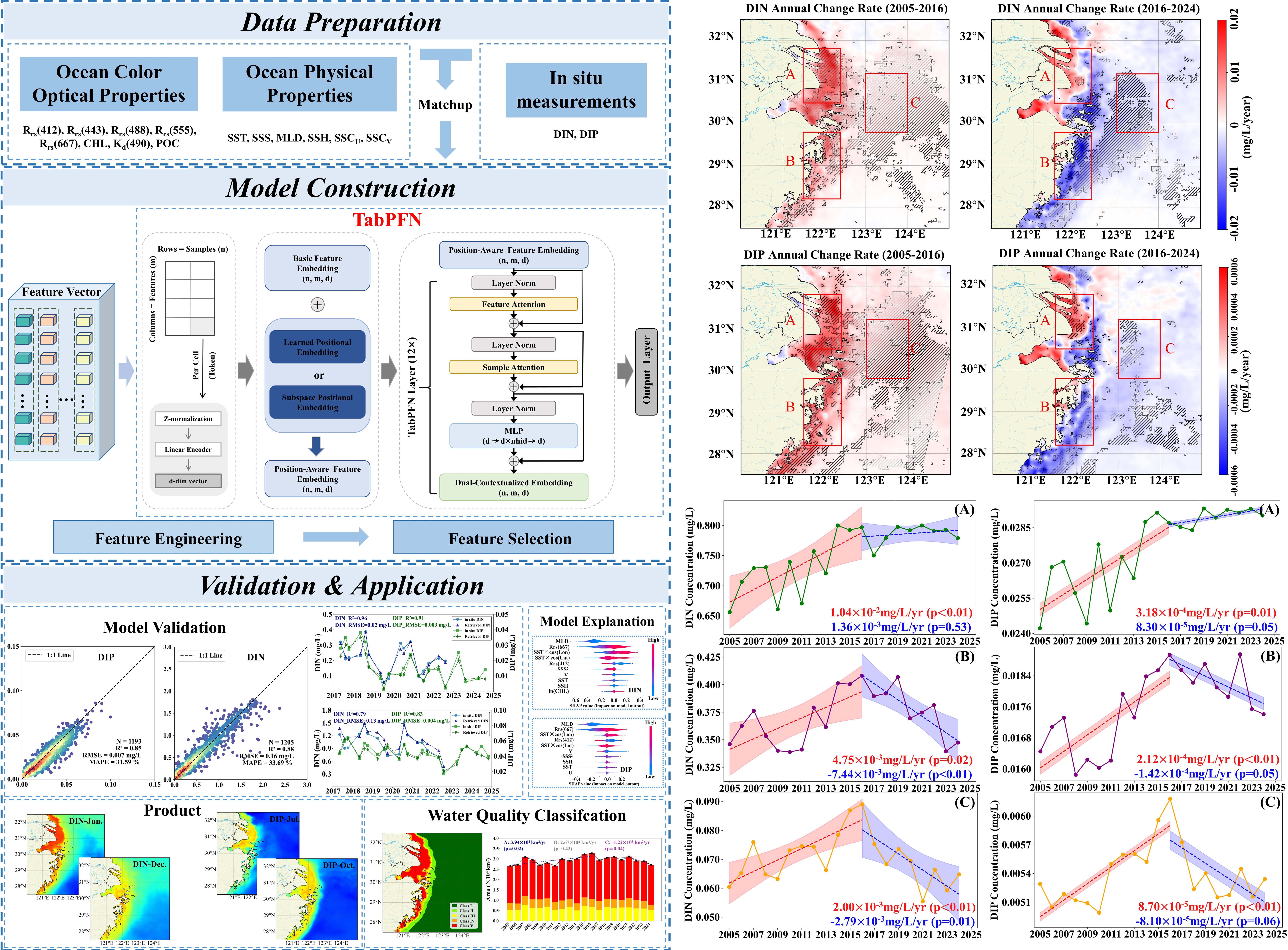
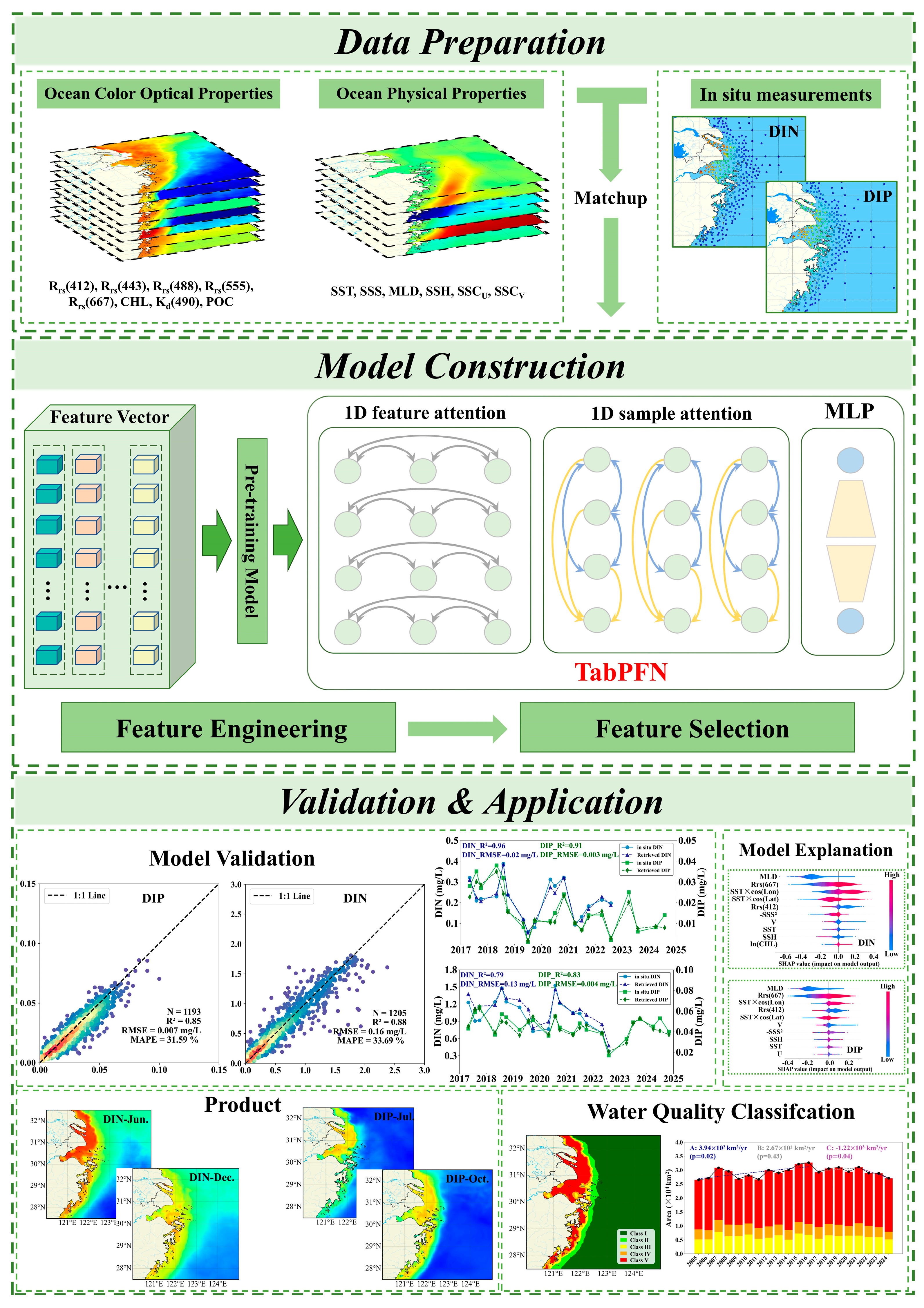
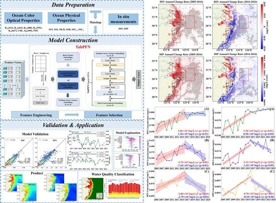
Graphical Abstract

1. Introduction

With the rapid development of industry and the continuous expansion of urban areas, anthropogenic disturbances have significantly increased the fluxes of nutrients such as nitrogen and phosphorus entering the ocean, thereby intensifying eutrophication in coastal waters [1,2,3]. Such nutrient enrichment frequently triggers environmental hazards, including algal blooms and red tides, resulting in reduced fishery yields and damaged tourism industries and causing economic losses on a global scale [4]. More seriously, deteriorated water quality may pose direct risks to human health through the bioaccumulation of harmful substances in the food chain [5]. Dissolved Inorganic Nitrogen (DIN) and Dissolved Inorganic Phosphorus (DIP) are widely recognized as key indicators for evaluating water pollution levels and diagnosing the state of marine ecosystems [6,7]. Therefore, accurate monitoring of DIN and DIP and a comprehensive understanding of their spatiotemporal dynamics are of great significance for water quality assessment and the development of environmental management strategies [8,9].
Traditional in situ monitoring of marine nutrients, while providing high accuracy, is constrained by substantial costs and time-consuming operations, especially for large-scale and long-term surveys [10]. In contrast, satellite remote sensing provides extensive spatial coverage and continuous observations, making it a valuable tool for acquiring the dynamic spatiotemporal information on marine nutrients [11]. Taking advantage of satellite observations, early studies employed multivariate linear regression to retrieve nutrient concentrations from optical remote sensing data. For example, Isenstein and Park [12] constructed regression models to estimate total phosphorus (TP) and total nitrogen (TN) in the Lake Champlain and Missisquoi Bay, while Yu et al. [9] applied multiple stepwise regression (MLSR) to estimate the DIN over the Bohai Sea based on the Moderate-resolution Imaging Spectroradiometer (MODIS) observations. Similarly, Mathew et al. [13] employed the MODIS data to assess TP and TN in the northern Arabian Sea. Conventional multivariate regression–based empirical models have ability to estimate the nutrient concentrations, but their retrieval accuracies are inherently limited, as nitrogen and phosphorus nutrients are non-optically active water quality parameters (WQPs) that affect water optical properties indirectly [14].
Recent developments in machine learning (ML), particularly deep learning (DL), have considerably enhanced the capability to retrieve nutrient concentrations from the remote sensing data. DL excels at capturing complex nonlinear relationships and has demonstrated strong performance in estimating WQPs [15,16,17], outperforming traditional empirical approaches. Currently, most ML-based nutrient retrieval studies have focused on inland waters [17,18,19], while several attempts have been made in marine waters. For example, Zhu et al. [6] developed classification and regression trees (CART) ML models to retrieve DIN, soluble reactive phosphate (SRP), and chemical oxygen demand (COD) in the Northern South China Sea (NSCS). However, due to the pronounced spatial heterogeneity of marine systems, regression relationships between nutrients and remote sensing satellite data generally vary by region, necessitating the development of dedicated models for specific marine areas [20]. Wu et al. [7] proposed an optimized deep belief network (DBN) incorporating spatiotemporal information to estimate DIN and DIP concentrations in the Zhejiang Coastal Sea. However, this model suffered from poor interpretability, functioning largely as a “black box”. In addition, despite progress in the Zhejiang coastal region, challenges of model accuracy, interpretability, and generalizability still remain in estimating nitrogen and phosphorus nutrients. Given these limitations, Transformer-based models and their variants have emerged as a promising alternative. Recent studies have increasingly explored their applications in ocean color remote sensing, demonstrating favorable accuracy and strong potential for retrieving water quality parameters [21,22].
Given the above considerations, this study develops an interpretable Transformer-based DL model to retrieve DIN and DIP concentrations in the Jiangsu-Zhejiang-Shanghai (JZS) offshore region, using satellite remote sensing and reanalysis datasets. The proposed framework will retrieve accurate and reliable DIN and DIP concentrations, reveal the spatiotemporal distribution characteristics of DIN and DIP in the JZS Offshore, and provide model interpretability by quantifying the contributions of input features to model outputs. This paper is structured as follows. Section 2 introduces the study area, data sources, processing and match-up methods, and model construction. Section 3 provides the results, including the validations of DIN and DIP, their seasonal characteristics and long-term changes, and water quality classification assessment. Finally, model interpretability, comparisons, and limitations are discussed in Section 4.

2. Data and Methods

2.1. Study Area

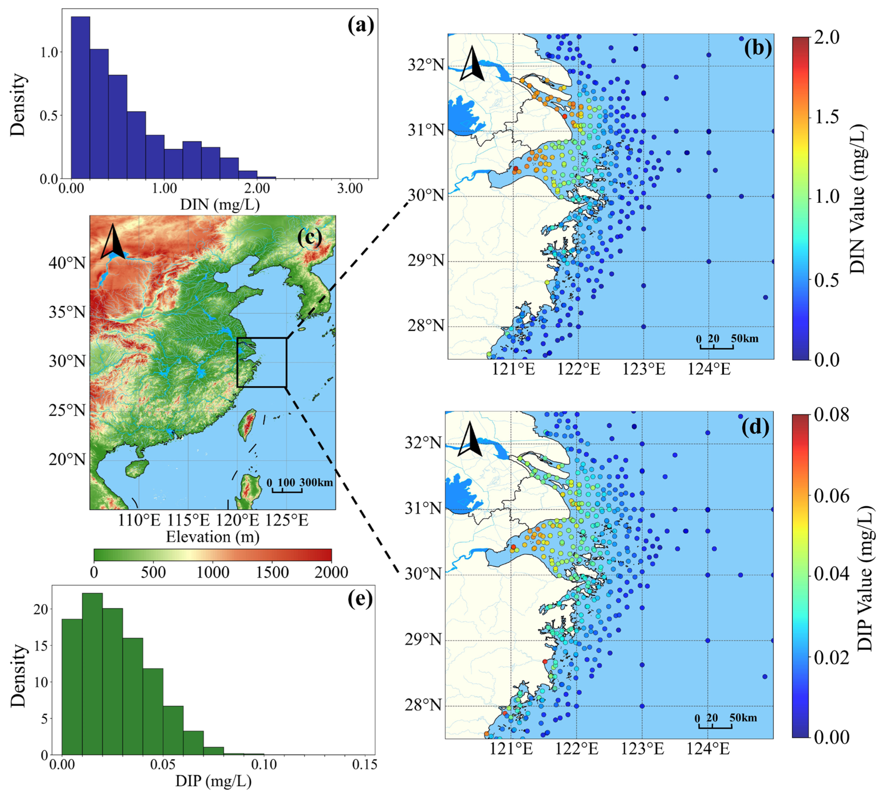
JZS offshore is located in the northern part of the East China Sea (ECS), spanning from 120°E to 125°E in longitude and 27.5°N to 32.5°N in latitude (Figure 1c). This area encompasses representative coastal and estuarine systems, including the Yangtze River Estuary and Hangzhou Bay, which have drawn considerable attention due to recurring eutrophication issues [23,24,25]. As the world’s third-largest estuary, the Yangtze River Estuary exhibits distinct hydrographic features such as the maximum turbidity zone and estuarine front [26]. Hangzhou Bay is one of the largest tidal bays globally, characterized by strong tidal dynamics that shape its unique hydrodynamic environment [27,28,29]. With the rapid population growth and industrial expansion in the Yangtze River Basin, nutrient enrichment and seawater eutrophication in the JZS offshore have been increasingly severe. Reports such as the Bulletin on the Ecological and Environmental Status of Zhejiang Province (https://sthjt.zj.gov.cn/art/2025/6/12/art_1229263297_5528655.html, accessed on 15 December 2025), together with relevant studies, consistently identify DIN and DIP as the primary water pollutants exceeding standard thresholds in this region [30,31].

2.2. Data Description

2.2.1. In Situ Measured Data

The in situ water quality observations employed in this study were derived from a comprehensive spatiotemporal dataset covering four decades (1980–2022) across China [32]. This dataset comprises more than 330,000 records of 18 water quality indicators collected from 2384 water quality monitoring sites. These sites are classified by monitoring frequency into daily (244 sites), weekly (149 sites), and monthly (1991 sites), with coverage extending across inland, coastal, and offshore waters.
For this study, the primary dataset used was the national monthly water quality records provided by NMEMC in the period of 2017–2022. The locations of monitoring sites and the mean values of the in situ measured DIN and DIP are shown as Figure 1b,d. Within the study region, DIN concentrations predominantly range between 0 and 2 mg/L (Figure 1a), while DIP concentrations fall mostly within 0–0.08 mg/L (Figure 1e). All data has undergone data cleaning and technical validation to ensure the consistency and scientific reliability. For data cleaning, geographical coordinate inconsistencies of the same monitoring site across different years were resolved by averaging longitude and latitude values, while duplicate records were removed to avoid redundancy. Missing data and empty entries were consistently coded as NA and excluded from the dataset, and values below the detection limits (0.001 mg/L for both DIN and DIP) were standardized and flagged as “<DL”. For technical validation, outliers were identified using the interquartile range (IQR) method where data points falling outside the range of Q1 − 1.5 × IQR to Q3 + 1.5 × IQR (Q1 denotes the first quartile and Q3 denotes the third quartile) were classified as outliers. Given that the number of available samples within the JZS Offshore was relatively limited, additional NMEMC records from 2023 and 2024 were incorporated. These supplemental datasets were exclusively used as training inputs for the retrieval model to alleviate underfitting and enhance model robustness.

2.2.2. Remote Sensing and Reanalysis Data

This study employed Level 3 satellite remote sensing products from the MODIS-Aqua sensor, obtained from the NASA Ocean Color Web (https://oceancolor.gsfc.nasa.gov/, accessed on 15 December 2025). Specifically, the ocean color remote sensing products utilized included CHL, SST, Rrs(412), Rrs(443), Rrs(488), Rrs(555), and Rrs(667), POC, and Kd(490). All datasets were processed under Version 2022.0, with a spatial resolution of 4 km. In addition, ocean reanalysis data were obtained from the Copernicus Marine Service (CMEMS) Data Store (https://data.marine.copernicus.eu/products, accessed on 15 December 2025). The selected variables included SSS, SSH, SSC, and MLD. The CMEMS products were provided at a spatial resolution of 1/12°, ensuring adequate representation of mesoscale oceanographic features relevant to nutrient dynamics. This study integrated in situ measured data, remote sensing data, and reanalysis products to predict DIN and DIP. The data sources and specific variables employed in this study were summarized in Table 1.

2.2.3. Data Processing and Match-Up

To address data gaps caused by cloud contamination and atmospheric correction errors in satellite observations, the Data Interpolating Empirical Orthogonal Function (DINEOF) method was applied to reconstruct missing values and ensure spatiotemporal continuity of the dataset [33]. For consistency, MODIS-Aqua remote sensing products (Rrs(λ), Kd(490), CHL, POC, and SST) and CMEMS reanalysis data (MLD, SSS, SSH, and SSC) were resampled to a spatial resolution of 1 km. Since NMEMC water quality measurements, remote sensing products, and reanalysis data are all monthly averages, the in situ DIN and DIP concentrations were matched to the nearest central pixel within a 1 km radius of each sampling point for the corresponding month. To minimize the influence of outliers in satellite-derived variables, an in situ measurement was deemed valid only when (i) more than ten valid pixels were available within a 5 × 5 pixel window, and (ii) the coefficient of variation across the window was less than 0.15. The 5 × 5 window provides a balanced spatial extent that effectively reduces sensor noise and small-scale anomalies while preserving physically meaningful environmental gradients in dynamic coastal waters like the Zhejiang Coastal Sea. The CV threshold of 0.15 filters out highly heterogeneous pixels that may result from sub-pixel contamination or unresolved fine-scale physical processes, thereby enhancing the reliability of the match-up dataset. These criteria are empirically supported and widely adopted in satellite ocean color studies over comparable marginal seas to ensure data quality for model development and validation [34,35]. Consequently, valid central grid cells and corresponding in situ WQPs concentrations were matched to construct the modeling dataset, resulting in a total of 5167 paired samples for DIN retrieval and 5058 paired samples for DIP retrieval, respectively.

2.3. Model Construction

The overall technical workflow of this study (Figure 2) comprises three stages: (i) data preparation, (ii) model construction, and (iii) validation and application. Specifically, data preparation includes two key steps: (1) acquisition of in situ measured data, remote sensing, and reanalysis data, and (2) data processing and matchup procedures. Model construction involves model training, feature engineering, and feature selection. The validation and application stage consists of three components: (1) model evaluation using statistical assessment metrics and interpretability analysis with SHapley Additive exPlanations (SHAP), (2) large-scale data production for the study area, and (3) water quality classification based on the generated outputs and established classification criteria.

2.3.1. Principle and Core Model

As typical non-optically active WQPs, DIN and DIP fail to directly absorb or scatter solar radiation in the visible spectrum (400–700 nm). Therefore, it proves incapable of accurately capturing the distribution patterns of DIN and DIP solely relying on optical characteristics. Instead, their spatiotemporal distributions are synergistically regulated by marine physical dynamic processes, biogeochemical cycles, and spatial geographical locations. To capture these indirect influences, two categories of input features were incorporated: ocean color properties (OCP, including Rrs(λ), Kd(490), CHL, and POC) and physio-chemical properties (PCP, including MLD, SSH, SSS, SST, and SSC). These predictors characterized the optical and physical conditions of the marine environment and were employed to model the nonlinear relationships with the target variables (DIN and DIP).
The core retrieval model is based on the Tabular Prior-data Fitted Network (TabPFN), a Transformer-based foundation model designed for small- to medium- scale tabular datasets [36]. TabPFN has been proven to have superior performance compared to the gradient-boosted decision tree (GBDT) like Categorical Boosting (CatBoost) and eXtreme Gradient Boosting (XGBoost), and the Automated Machine Learning systems (AutoML), achieving competitive regression accuracy while reducing training time by several orders of magnitude [36]. Generally, TabPFN delivers a speedup of up to a 3000× on datasets containing fewer than 10,000 samples and 500 features, alongside robust performance against outliers, uninformative features and missing values that are frequently encountered in real-world tabular regression scenarios. Feature normalization and missing-value handling are internally implemented in TabPFN through z-normalization and indicator-based imputation, respectively. When evaluated on the regression benchmarks, TabPFN improved normalized RMSE by 0.051 under default settings and by 0.093 after tuning compared with the CatBoost [36], underscoring its effectiveness beyond computational efficiency.
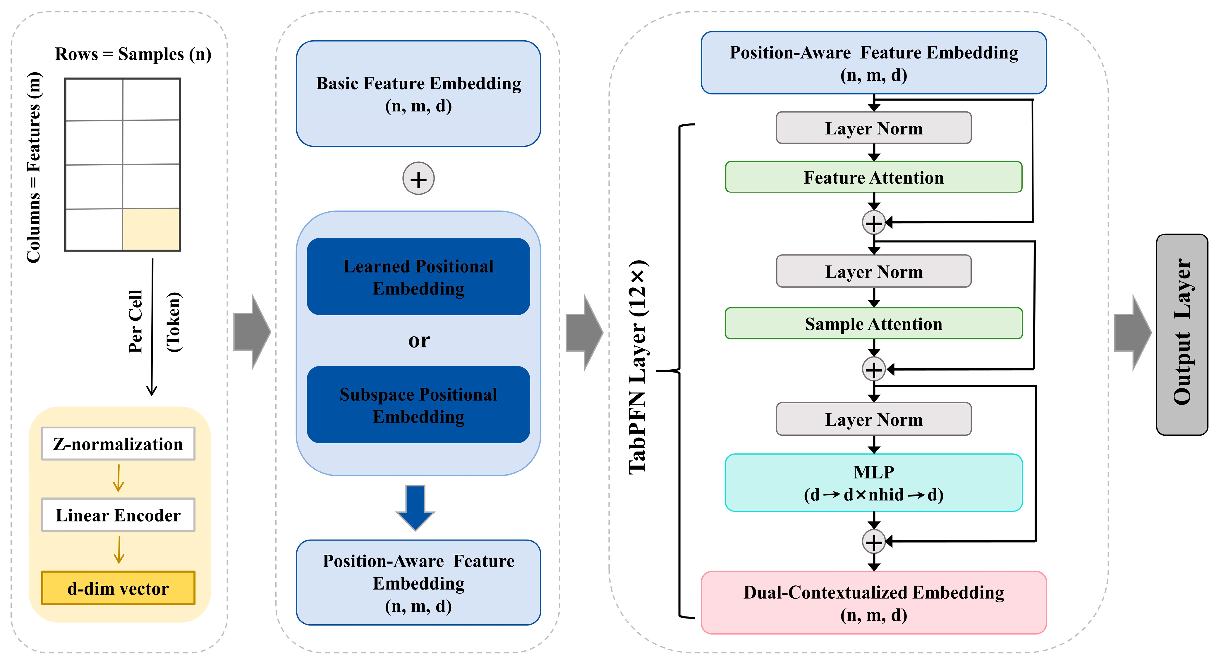
Unlike conventional Transformers that primarily process sequential data, TabPFN (architecture is illustrated in Figure 3) leverages a dual-attention mechanism optimized for tabular structures. At the intra-sample level, each feature attends to other variables within the same record to capture contextual relationships across predictors, while at the inter-sample level, attention is applied across rows for each feature, allowing the model to learn population-level patterns [36]. Furthermore, TabPFN was pretrained on millions of synthetic datasets generated through structural causal models, which not only enhanced generalization but also mitigated the risks of privacy leakage and data contamination associated with conventional foundational models [36]. During application, predictions are completed in a single forward pass by conditioning on the available feature set and unmasked samples. TabPFN is highly suitable for this study because the features (OCP and PCP) and the target variable (DIN and DIP) naturally form tabular structures, and the dataset size of the JZS Offshore region falls within the range where TabPFN exhibits its strongest advantages. Hence, TabPFN provides both computational efficiency and predictive robustness, making it an ideal choice for DIN and DIP retrieval. To further validate the advantages of TabPFN over mainstream ML models, this study constructed DIN and DIP retrieval models based on Random Forest (RF), XGBoost and Light Gradient Boosting Machine (LightGBM) using the same datasets.

2.3.2. Feature Engineering and Selection

Feature engineering in this study included classical mathematical transformations and spectrum-based transformations of predictor variables [37]. The former involved reciprocal, logarithmic, exponential, square root, and square operations, while the latter involved band normalization and two-band or three-band combinations. These mathematical operations were applied to both OCP and PCP in this study, thereby enriching the feature space. The algorithms used for the transformation are summarized in Table 2.
All parameters processed through feature engineering, along with the raw parameters (i.e., those not subjected to feature engineering), were initially included as candidate inputs for the model construction. To select the most effective features, the mean absolute percentage error (MAPE) is employed to rank and filter the features. The calculation formula of MAPE is as follows:
MAPE ( % ) = 1 n i = 1 n y i y ^ i y i × 100 %
where y i and y ^ i represent in situ measured and estimated values, respectively, and n represents the number of samples. In practice, random perturbations were introduced to a specified feature variable to update the input features, while keeping other features constant. A new model was constructed using these updated features, and its MAPE was calculated. If the resulting MAPE was greater than that of the baseline model, the feature was deemed effective.
The importance scores of all variables were calculated and ranked in descending order. Features were sequentially selected based on the list, ultimately yielding an appropriate set of input features to construct the optimal model. Detailed descriptions of the feature engineering and selection procedures are shown in Text S1 of Supplementary Materials. In this study, input features were randomly partitioned into training and validation subsets using stations as the grouping unit, with a baseline split ratio of 8:2. When a station contained a limited number of samples, the split ratio was reduced to ensure that the observations from each station were represented in both the training and validation datasets. As monthly average CMEMS and MODIS-Aqua products were used and the TabPFN model was trained to learn nonlinear input–output relationships, no additional region-specific outlier filtering was applied in this study.

2.3.3. SHAP Interpretability

Model interpretability was achieved using the SHAP tool, a post hoc explanatory method that quantified the marginal contribution of each feature to the model prediction [38,39]. As one of the most effective approaches for model interpretation [40], SHAP was employed to investigate the explainable mechanisms of TabPFN in estimating DIN and DIP concentrations. The model produced a predictive value for each sample, and the SHAP value was a quantity assigned to each feature within the sample, accounting for specific contribution of the feature toward predictive output of the model.
In addition to quantifying the magnitude of feature contributions, SHAP further revealed the direction (positive or negative) of the relationships between predictors and target variables [41,42]. A positive SHAP value (>0) indicates that the feature increases the predicted value of the target parameter, whereas a negative value (<0) denotes a suppressing effect. Therefore, SHAP enables the disentanglement of both direction and strength of feature contributions [43,44].

2.3.4. Accuracy Assessment

To assess the accuracy of the retrieval model, three widely used statistical metrics indices were adopted: MAPE, root mean square error (RMSE), and coefficient of determination (R2). Their specific mathematical expressions are given in Equations (1)–(3).
RMSE = 1 n i = 1 n ( y i y ^ i ) 2
R 2 = 1 i = 1 n ( y i y ^ i ) 2 i = 1 n ( y i y ¯ ) 2
where y i and y ^ i represent in situ measured and estimated values, respectively, y ¯ denotes the mean of observed values, and n is the number of samples.
To further assess predictive stability, residuals between in situ observations and model estimates were calculated, and their dispersion was quantified using the standard deviation of residuals (Std Residual) was used to quantify the stability of the model:
Std   Residual = 1 n 1 i = 1 n ( r i r ¯ ) 2
where r i is the residual for the i-th sample, and r ¯ is the mean residuals. A smaller Std Residual indicates a narrower residual distribution and, consequently, greater stability of model predictions.

2.4. Water Quality Classification Criterion

This study adopted the single-factor assessment method (https://mee.gov.cn/, accessed on 15 December 2025) to evaluate seawater quality with reference to the National Seawater Quality Standard of the People’s Republic of China (GB 3097-1997). In this method, the classification thresholds were defined separately for DIN and DIP. For DIN: concentrations ≤ 0.2 mg/L correspond to Case I, 0.2 < DIN ≤ 0.3 mg/L to Case II, 0.3 < DIN ≤ 0.4 mg/L to Case III, 0.4 < DIN ≤ 0.5 mg/L to Case IV, and DIN > 0.5 mg/L to Case V. For DIP: concentrations ≤ 0.015 mg/L correspond to Case I, 0.015 < DIP ≤ 0.03 mg/L to Case II or III, 0.03 < DIP ≤ 0.045 mg/L to Case IV, and DIP > 0.045 mg/L to Case V. The overall water quality classification of a given region was determined by the worst-performing indicator among all individual WQPs.

3. Results

3.1. Model Validation

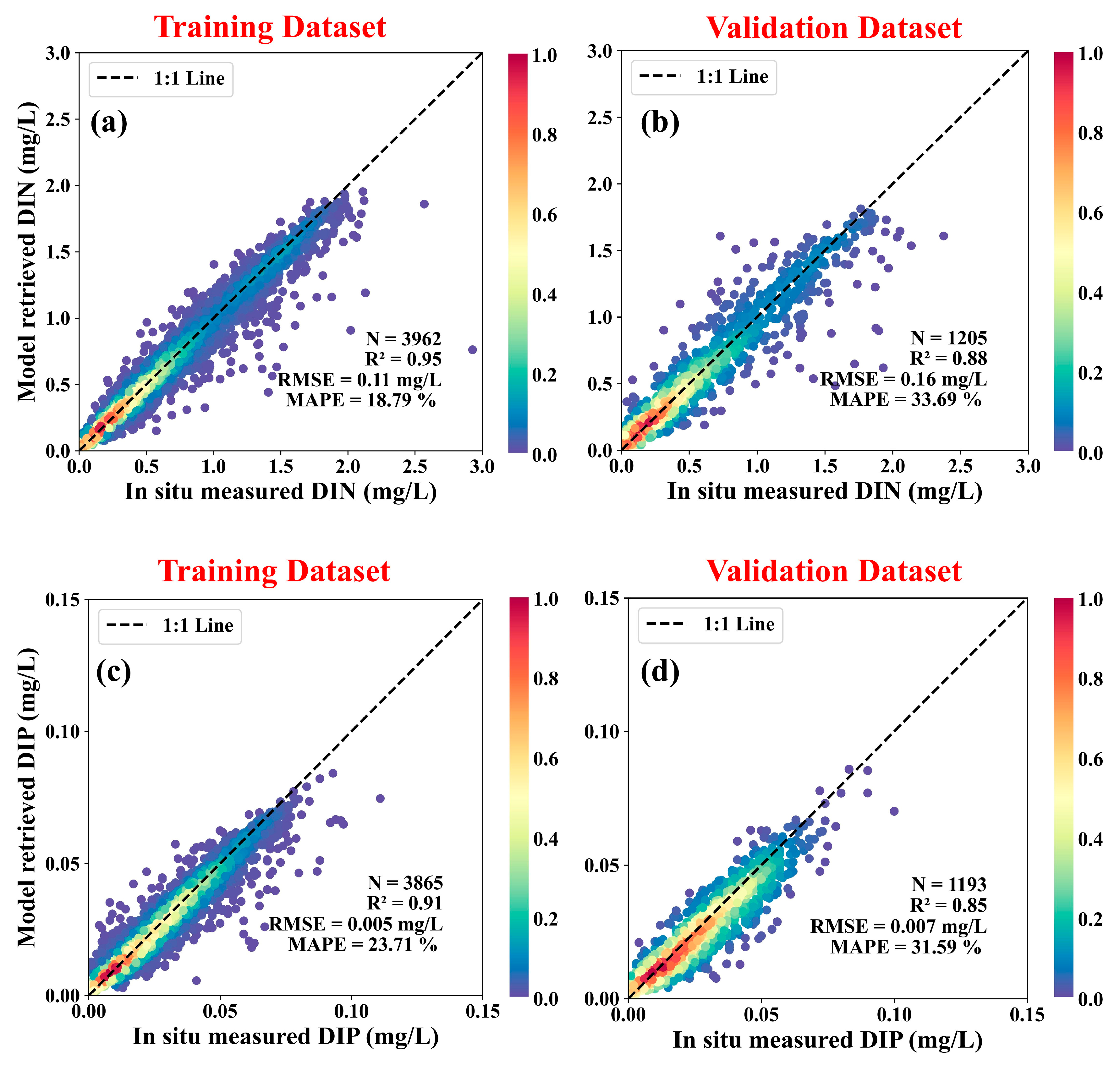
Using remote sensing and reanalysis data as inputs, TabPFN produced DIN and DIP predictions through a single forward propagation. Compared with RF, XGBoost, and LightGBM, TabPFN has been demonstrated to outperform these models on small-to-medium-sized datasets. Specifically, it achieves the highest R2 values and lowest MAPE and RMSE values in both DIN and DIP predictions (Table 3). Furthermore, the predicted values of TabPFN are uniformly distributed around the 1:1 line in Figure 4, indicating a high level of predictive accuracy. On the training dataset, R2 values for DIN and DIP reached 0.95 and 0.91, with RMSE values of 0.11 mg/L and 0.005 mg/L, and MAPE values of 18.79% and 23.71%, respectively. As for the validation dataset, R2 values remained high at 0.88 for DIN and 0.85 for DIP, accompanied by RMSE values of 0.16 mg/L and 0.007 mg/L, and MAPE values of 33.69% and 31.59% (Figure 4b,d). Notably, the distribution of scatter points is concentrated in the low-value regions (below 0.02 mg/L) of DIP, whereas higher DIP concentrations (over 0.08 mg/L) tend to be underestimated, with points scattered below the 1:1 line (Figure 4d). Nonetheless, the clustering of high-density scatter points is all located near the 1:1 line, indicating that the TabPFN model effectively captured the nonlinear relationships between WQPs with remote sensing inputs. The slight differences in RMSE and MAPE between the training and independent validation datasets further confirm the model robustness and generalizability.
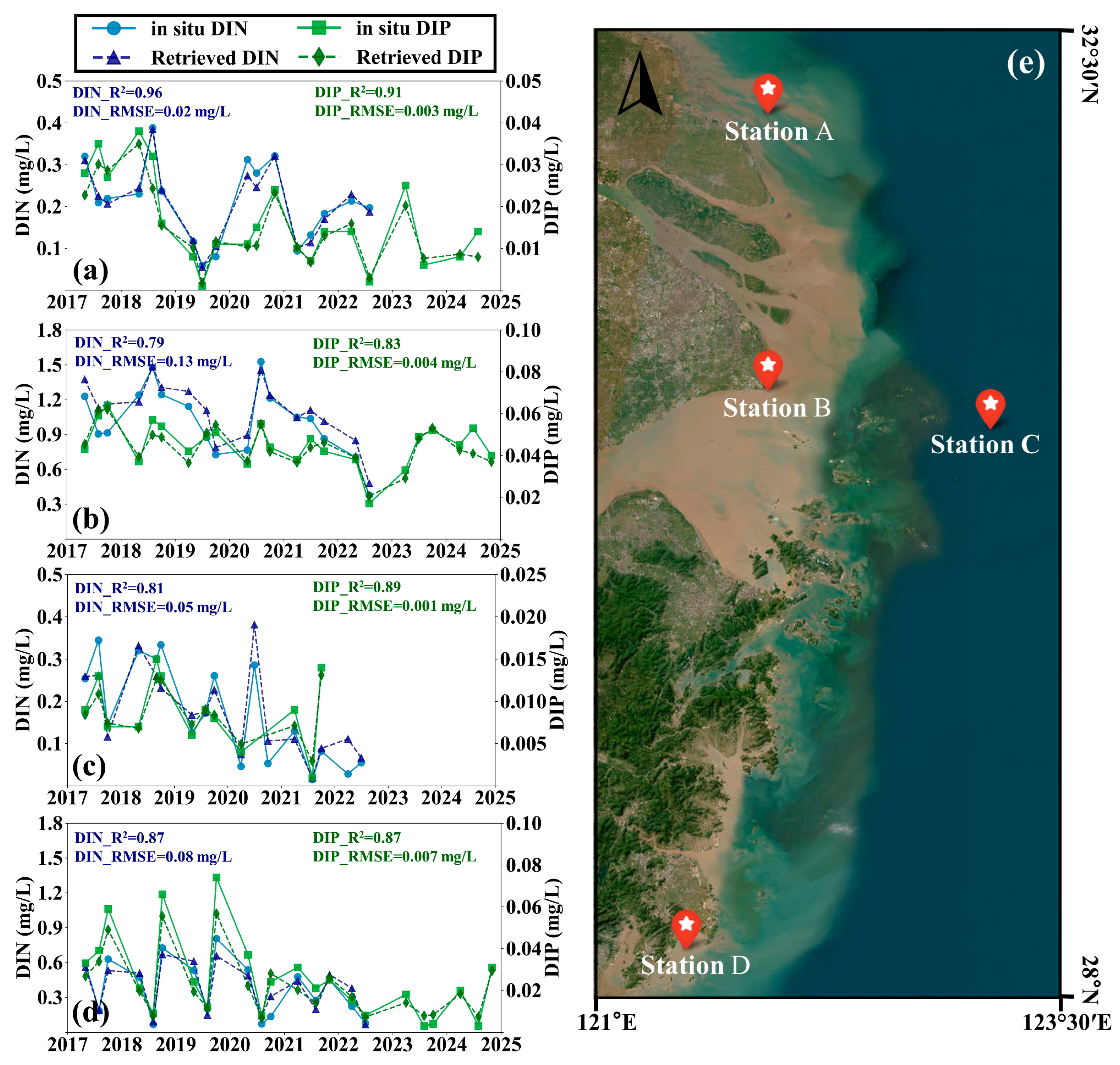
To assess station-level accuracy, four in situ monitoring sites (Stations A–D) with multi-year observations (2017–2022) were selected for time-series validation (Figure 5). The time-series comparison of the four stations revealed strong agreement between TabPFN retrievals and the in situ measurement, with relatively high R2 ≥ 0.79 and RMSE ≤ 0.13 mg/L for DIN and RMSE ≤ 0.007 mg/L for DIP across all stations. Notably, the R2 values of DIN and DIP at Station A reached as high as 0.96 and 0.91, respectively, with the corresponding RMSE values of 0.02 mg/L and 0.003 mg/L (Figure 5a). These results underscore the excellent accuracy and reliability of the TabPFN in station-level applications.
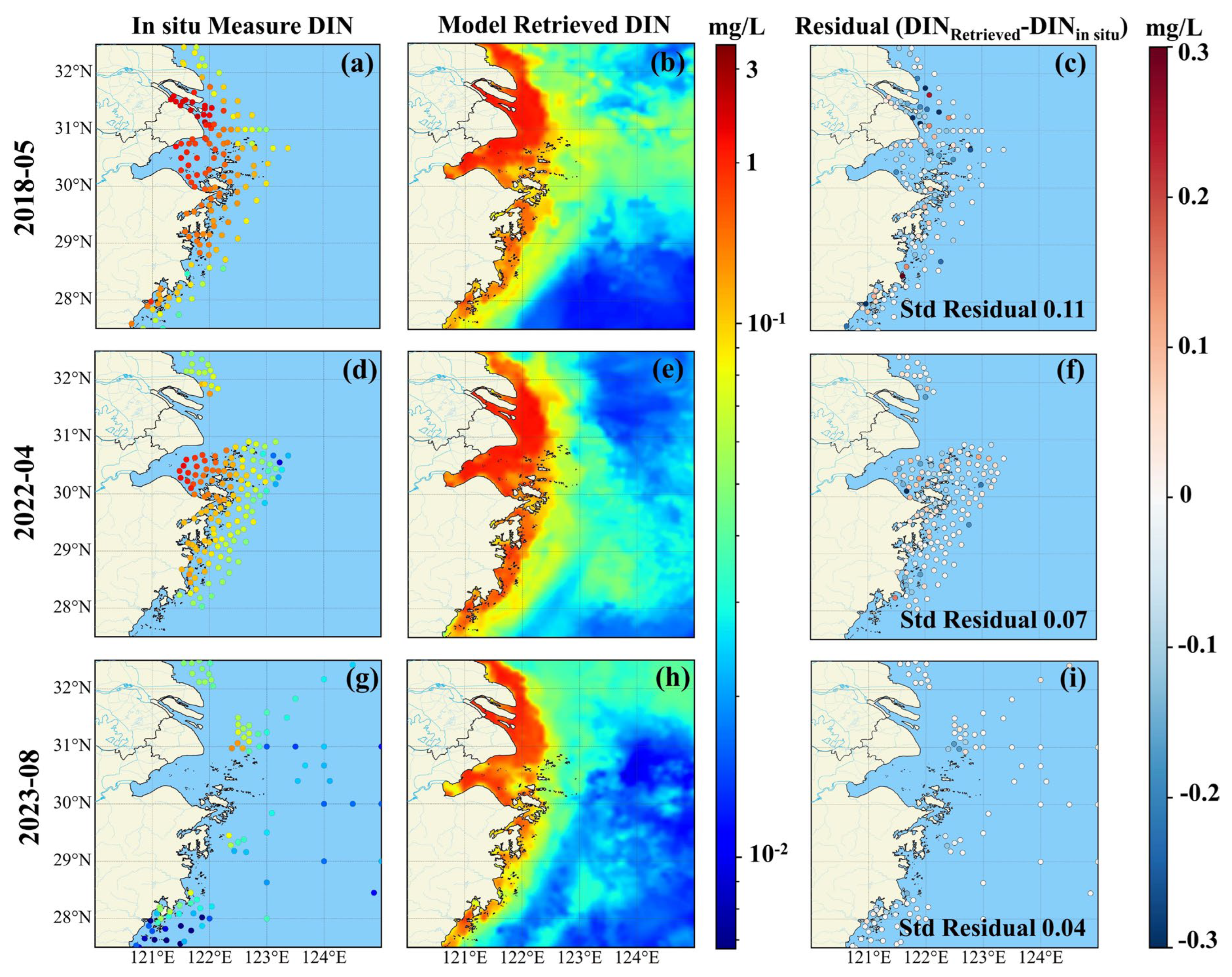
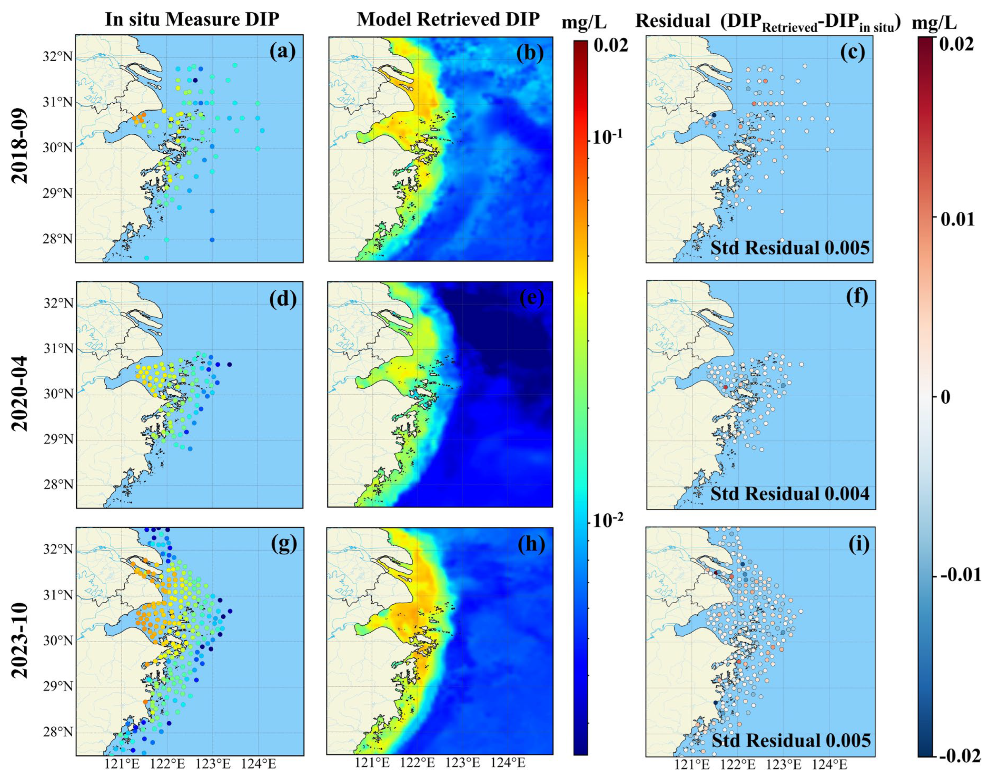
To further evaluate the spatial consistency of the remote sensing products for DIN and DIP, we selected the retrieval results for three months to compare with in situ station observations, as shown in Figure 6 and Figure 7. In detail, the months selected for DIN are May 2018, April 2022, and August 2023, and those for DIP are September 2018, April 2020, and July 2022. The selected months ensured adequate station coverage across estuarine, nearshore, and offshore environments. The predicted spatial distributions (Figure 6b,e,h and Figure 7b,e,h) closely matched the in situ observations (Figure 6a,d,g and Figure 7a,d,g), with residuals largely approaching zero. Specifically, the residuals of DIN were concentrated within −0.1 to 0.1 mg/L, and those of DIP within −0.005 to 0.005 mg/L, indicating high retrieval accuracy.
The high-value (>0.2 mg/L) and low-value (<0.2 mg/L) regions in Figure 6c,f,i are mainly localized in the Yangtze River Estuary, southern Hangzhou Bay, and the Zhejiang coast, while offshore stations exhibited minimal residuals, reflecting stronger model performance in open waters. Furthermore, the Std Residual values of DIN at the in situ measurement stations for the three corresponding time points were all less than 0.11, while those of DIP at the in situ stations for its corresponding time points were all less than 0.005, confirming the high stability of TabPFN across different time periods and marine environments.

3.2. Seasonal Variation Characteristics

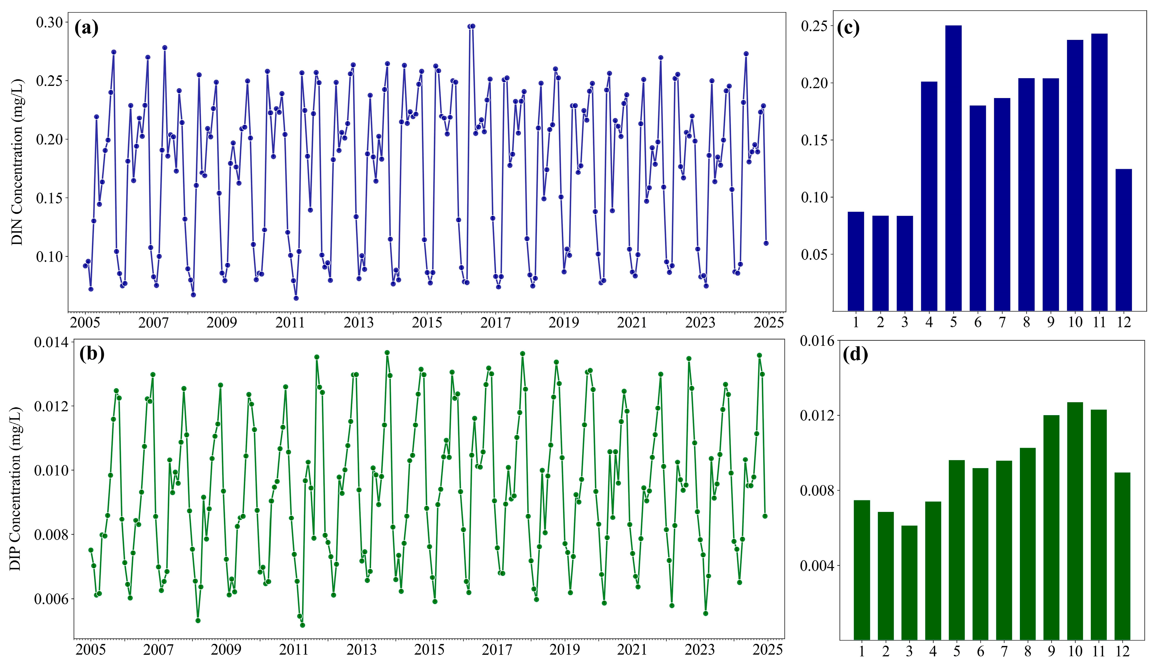
To investigate the seasonal dynamics and long-term changes in DIN and DIP in the JZS Offshore, TabPFN was applied to reconstruct nutrient concentration values from 2005 to 2024. The long-term time series (Figure 8a,b) reveal distinct seasonal cycles for DIN and DIP, characterized by regular intra-annual fluctuations and interannual variability. DIN concentrations (Figure 8a) typically ranged between 0.08 and 0.30 mg/L, while DIP concentrations (Figure 8b) varied from approximately 0.005 to 0.014 mg/L. The monthly climatologies (Figure 8c,d) show that DIN concentrations were lowest in March (0.08 mg/L) and peaked in May (0.25 mg/L). Seasonally, DIN concentration is the lowest in winter (December to February), while it reaches the highest in autumn (September to November). DIP exhibited a similar but less pronounced seasonal pattern, with minimum values in winter (0.006 mg/L) and maximum values in autumn (0.013 mg/L).
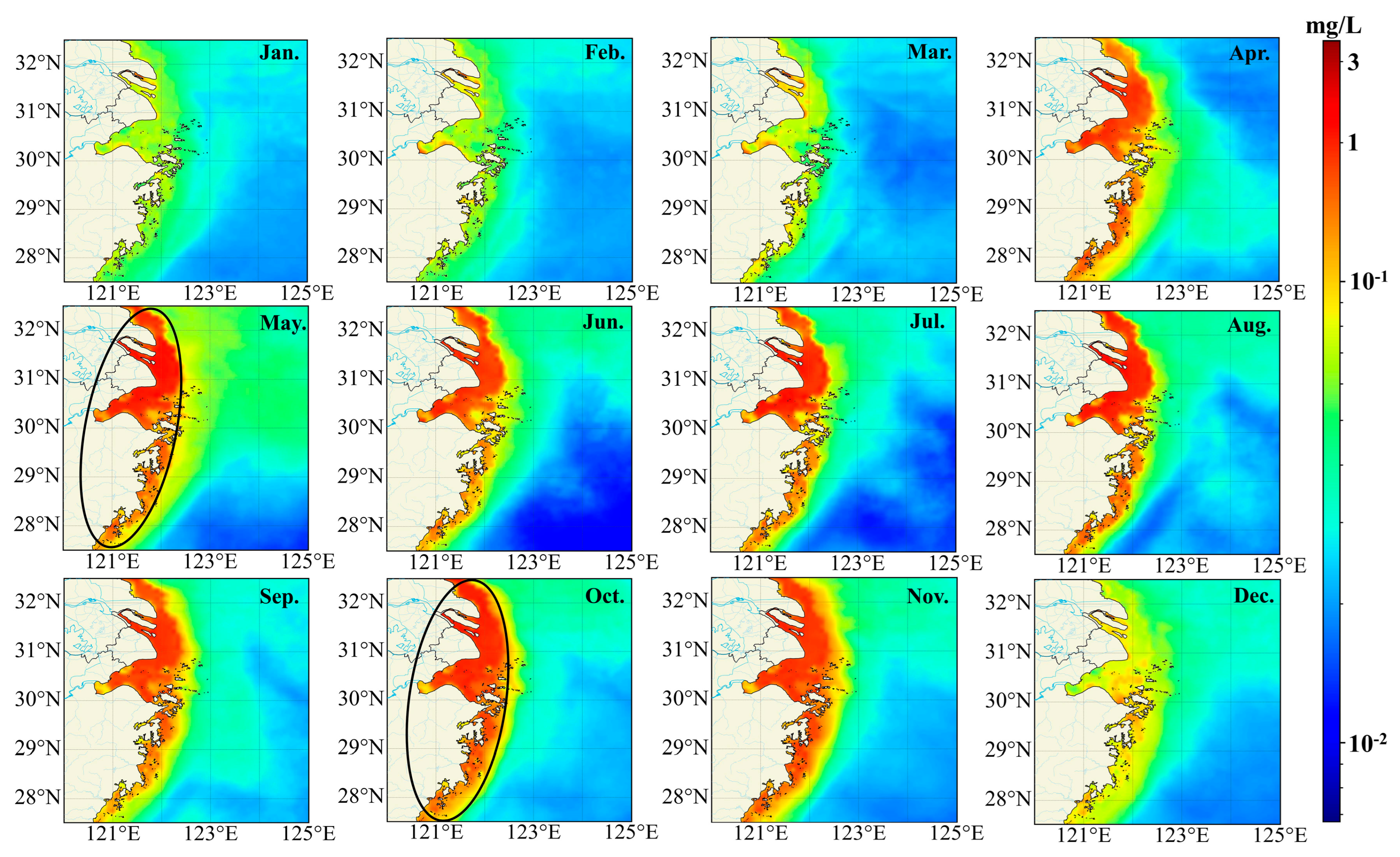
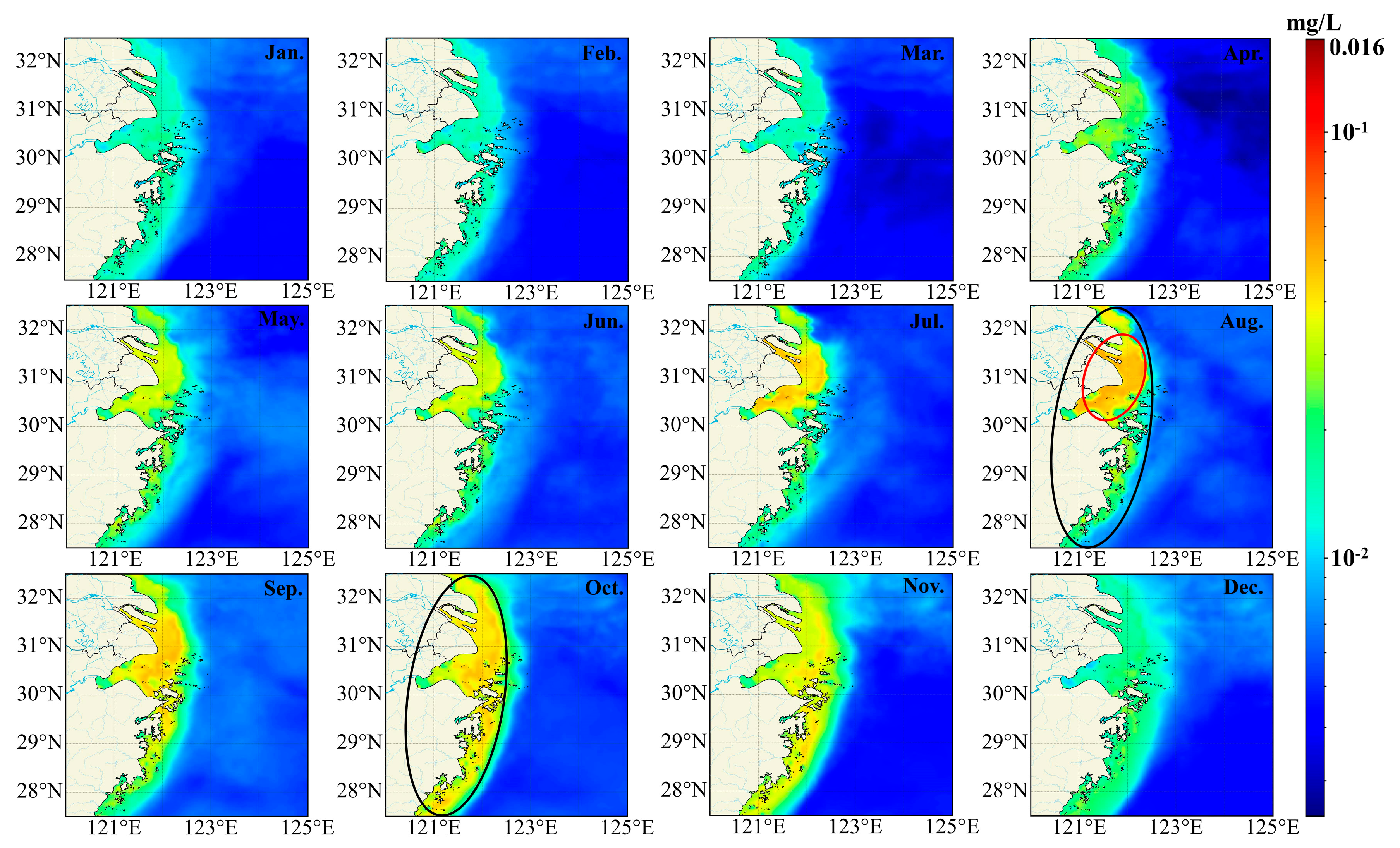
Figure 9 and Figure 10 illustrate the spatial distributions of monthly DIN and DIP retrievals in the JZS Offshore over the past 20 years. Overall, DIN and DIP both exhibited a characteristic estuarine–offshore gradient, with relatively high concentrations (more than 1.5 and 0.06 mg/L for DIN and DIP, respectively) in the estuarine and nearshore waters (highlighted by black ellipses), followed by a gradual decrease toward the open ocean. This spatial pattern reflects the strong influence of terrestrial inputs and estuarine hydrodynamics on nutrient distributions.
As shown in Figure 9, the spatial pattern of monthly DIN shows that in months with high concentrations (mean value over 0.2 mg/L), estuary and nearshore waters exhibit relatively homogeneous distributions, with nutrient levels broadly elevated across the region. In contrast, offshore waters exhibit markedly lower concentrations, with weaker temporal variability. The monthly changing rates of DIN in the estuarine and nearshore areas are considerably higher than that observed in offshore waters, highlighting the dominant role of riverine discharge and anthropogenic inputs in driving temporal fluctuations. Seasonal differences are also evident, with estuarine and nearshore DIN concentration falling below approximately 0.1 mg/L from December to March, whereas offshore low concentrations (less than 0.04 mg/L) are more pronounced during summer months, particularly in June and July, likely due to the intensified stratification and dilution effects.
The spatial distribution of DIP (Figure 10) exhibits pronounced seasonal variability, with higher concentrations (over 0.03 mg/L) mainly confined to estuarine and nearshore waters. Elevated DIP levels (more than 0.04 mg/L) are evident from May to October, particularly around the Yangtze River Estuary and Hangzhou Bay (highlighted by red ellipses), indicating strong terrestrial and anthropogenic influences. In summer (July–September), high DIP patches expand southward along the Zhejiang coast, while in winter (December–February), DIP concentration declines substantially across most coastal regions, reflecting reduced riverine inputs and enhanced vertical mixing. Offshore waters generally maintain low DIP concentration (less than 0.006 mg/L) throughout the year, suggesting limited nutrient transport from nearshore areas. These seasonal patterns collectively suggest that the DIP is predominantly governed by river discharge, coastal circulation, and biological uptake processes.

3.3. Long-Term Trend

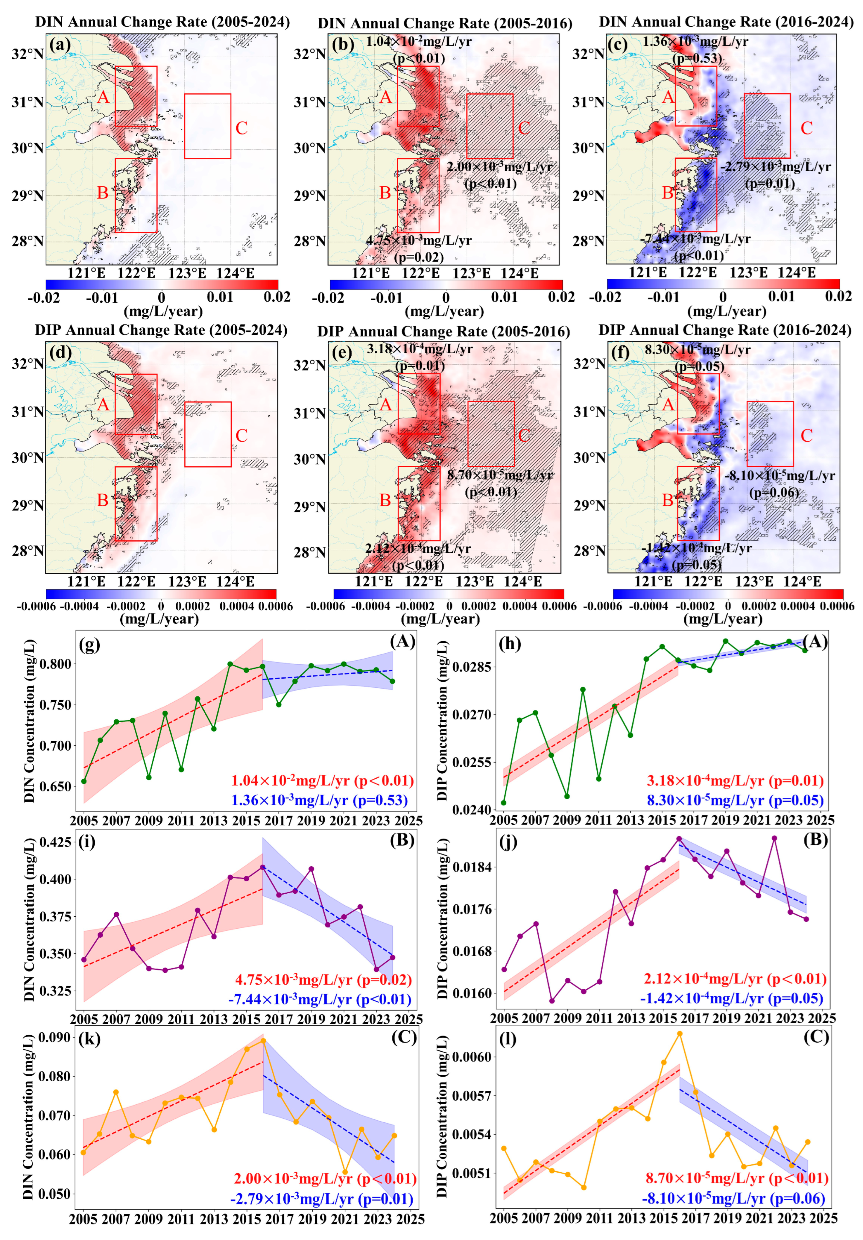
Figure 11 presents the spatial and temporal distributions of the long-term trends in model-derived DIN and DIP over the JZS Offshore. From 2005 to 2024 (Figure 11a,d), DIN and DIP both exhibited increasing trends across most coastal waters, particularly along the northern and central coastal waters (regions A and B), indicating sustained nutrient enrichment over the past two decades. The trend patterns in the period from 2005 to 2016 (Figure 11b,e) reveal widespread positive rates of changes in DIN and DIP, with evident increases occurring near the river estuaries and coastal waters, suggesting strong terrestrial influence during 2005–2024. In contrast, the spatial distributions of the variation trends of DIN and DIP during 2016–2024 (Figure 11c,f) present distinct transition, with decreasing trends dominating the offshore and southern waters, reflecting the effectiveness of recent pollution mitigation efforts and the resulting improvement in water quality.
Figure 11g–l illustrate the interannual changes in DIN and DIP concentrations in regions A–C. As for the region A (Figure 11g,h), DIN and DIP both exhibited significant upward trends during 2005–2016, with annual increases of 1.04 × 10⁻² mg/L/yr (p < 0.01) and 3.18 × 10⁻⁴ mg/L/yr (p = 0.01), respectively. In region B (Figure 11i,j), nutrient variations displayed turning pattern, with DIN and DIP increased significantly before 2016 (4.75 × 10⁻³ mg/L/yr and 2.12 × 10⁻⁴ mg/L/yr, respectively) but showed decreasing trends afterward (–7.44 × 10⁻³ mg/L/yr for DIN and –1.42 × 10⁻⁴ mg/L/yr for DIP). For the region C (Figure 11k,l), DIN and DIP exhibited similar temporal trends, with significant increases during 2005–2016 (2.00 × 10⁻³ mg/L/yr for DIN and 8.70 × 10⁻⁵ mg/L/yr for DIP, p < 0.01), followed by declines from 2016 to 2024 (–2.79 × 10⁻³ mg/L/yr and −8.10 × 10⁻⁵ mg/L/yr, respectively). The trend slops and significance levels across the aforementioned regions are detailed in Table 4. The spatiotemporal changes in DIN and DIP indicate that the nutrient enrichment strengthened in the previous twelve years (2005–2016) but has declined in the recent eight years due to the improved pollution control and management.

3.4. Water Quality Classification Assessment

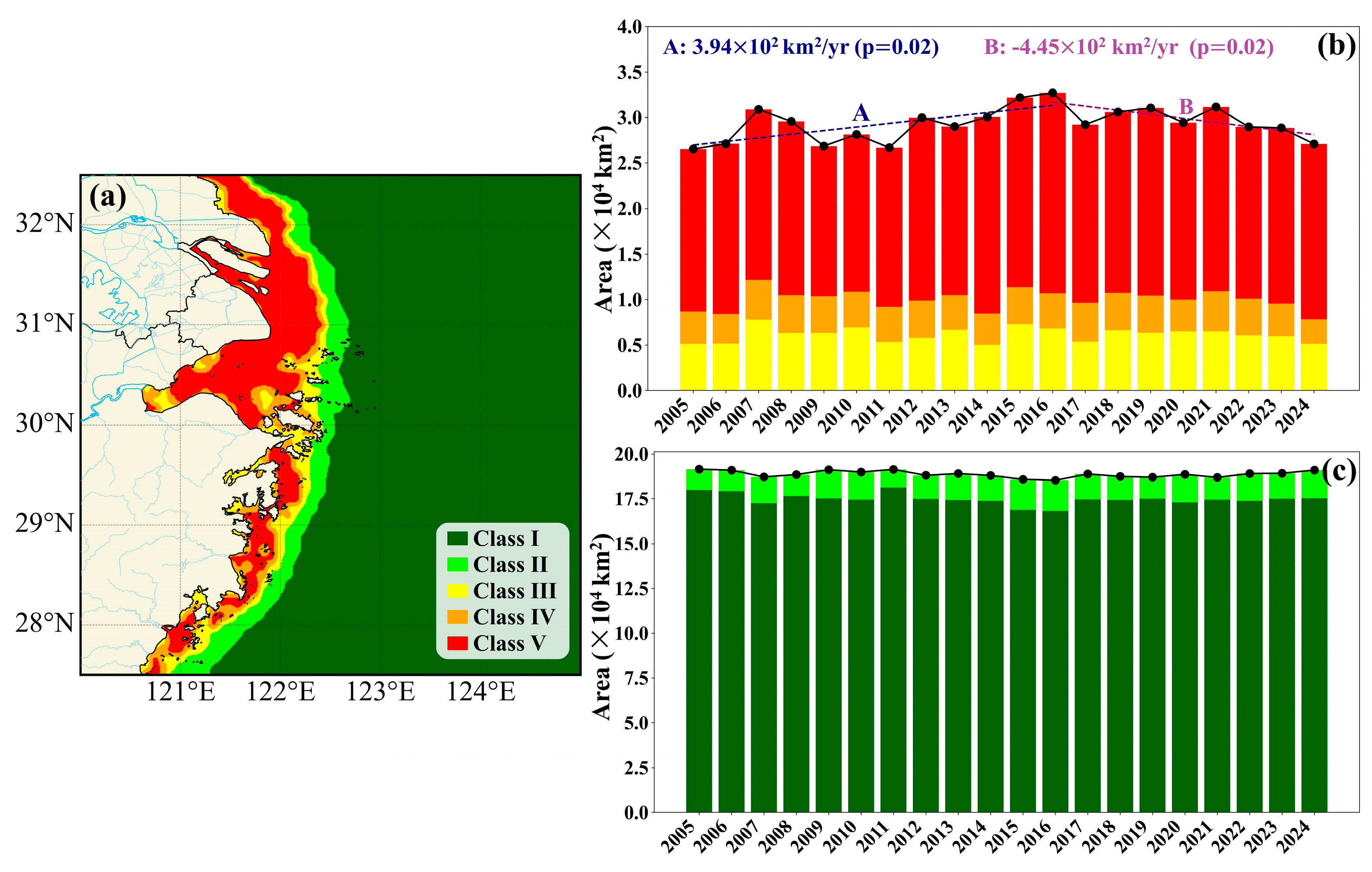
Based on the DIN and DIP derived from remote sensing retrieval, the water quality in the JZS region was classified in accordance with the National Seawater Quality Standard of the People’s Republic of China (GB 3097-1997), and the classification results are presented in Figure 12. Spatially, the water quality levels in the JZS offshore waters (Figure 12a) exhibit a distinct gradient, decreasing progressively from the estuarine and nearshore areas toward the open ocean. Case I waters occupy the largest proportion of the study area, followed by Case V, whereas Cases III and IV, which represent the transitional conditions between polluted and clean waters, cover the smallest areas. In particular, the estuary and nearshore regions were predominantly categorized as Cases III, IV, and V, indicating eutrophication and nutrient enrichment, while the offshore waters were dominated by Cases I and II. These spatial patterns basically align with the annual Bulletin on the Status of Marine Ecological Environment published by NMEMC (https://www.nmemc.org.cn/hjzl/sthjgb/202509/P020250910537280063392.pdf, accessed on 15 December 2025).
For analytical clarity, the water quality classifications were further consolidated into two categories: high-quality waters (Cases I and II) and medium-to-high eutrophic waters (Cases III, IV, and V). Specifically, waters were classified as medium-to-high eutrophic waters when DIN concentration exceeded 0.3 mg/L or DIP concentration exceeded 0.03 mg/L, while the remaining waters were defined as high-quality waters. A long-term temporal assessment (Figure 12b) indicates that the spatial extent of medium-to-high eutrophic waters showed an increasing trend from 2005 to 2016, with a rate of 3.94 × 10² km2/yr (p = 0.02). After 2016, the increasing trend transitioned into a significant decline (−4.45 × 10² km2/yr during 2016–2024, p = 0.02), suggesting notable improvement in coastal water quality during this period. Conversely, the areal extent of high-quality waters (Figure 12c) exhibited an inverse trend, remaining dominant throughout the study period and exhibiting slight expansion in recent years. The observed changes suggest a gradual transition toward better water conditions in the JZS Offshore in the past decade, consistent with recent improvements in coastal environmental management.

4. Discussion

4.1. Model Interpretability

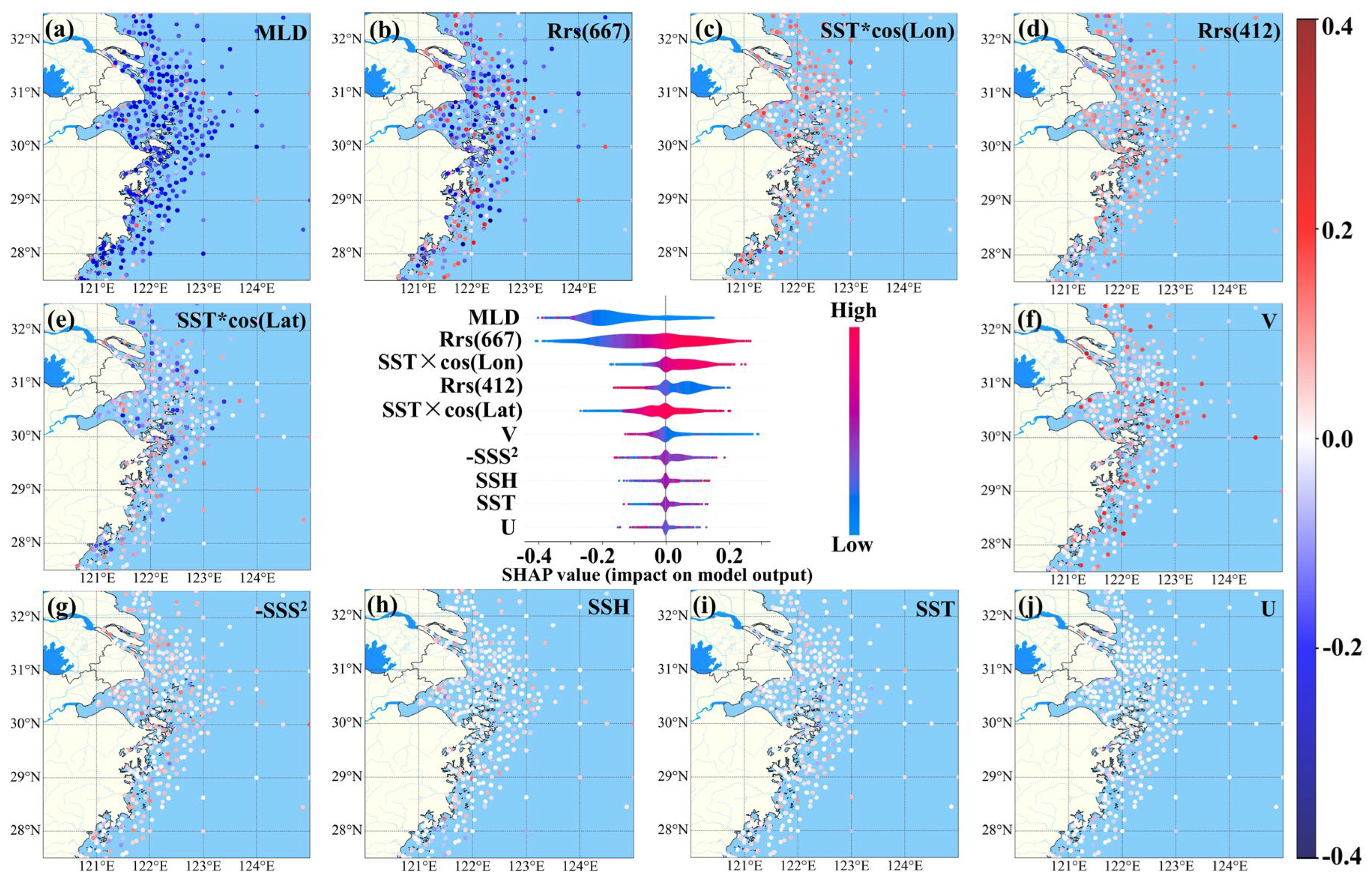
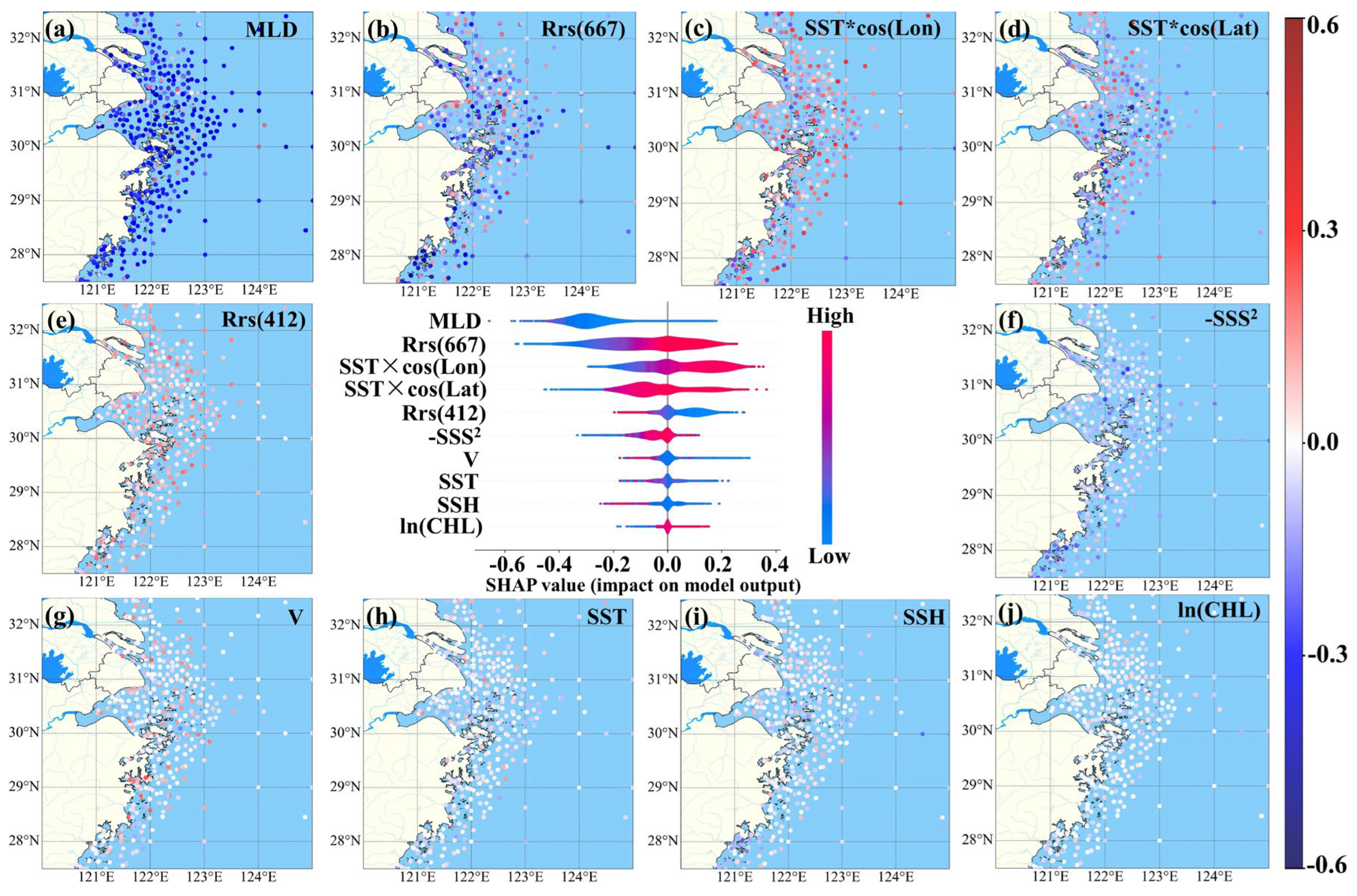
Figure 13 and Figure 14 illustrate the contribution of the first ten most influential input features to the model output, together with the corresponding SHAP value distributions for each feature (Figure 13a–j and Figure 14a–j), respectively. Among these variables, the constructed indices SST × cos(Lat and SST × cos(Lon) effectively capture the role of geographical location in modulating nutrient dynamics. Specifically, SST × cos(Lon) reflects the cross-shore gradient associated with coastal currents, while SST × cos(Lat) characterizes the latitudinal modulation of temperature effects.
For the TabPFN-DIN model (Figure 13), the variations in DIN in JZS Offshore are mainly controlled by MLD, Rrs(667), Rrs(412), SST × cos(Lon), and SST × cos(Lat). MLD exhibits predominantly negative SHAP values (below −0.3), reflecting the effect of water stratification, as deeper mixed layers promote vertical mixing that dilutes surface nutrients and lowers DIN, consistent with the in situ observations [45]. To further quantify the spatial heterogeneity of feature contributions, the study area was divided into 1° × 1° latitude-longitude grid cells, and the dominant positive and negative features influencing DIN were analyzed for each cell (Figure S1a,b in Supplementary Materials). This grid-based quantitative analysis confirms MLD as the consistent negative dominant feature for DIN across the entire study area, with the average negative SHAP value of MLD in each grid cell being lower than −0.23 (Figure S1a). These results quantitatively confirm the robust inhibitory effect of MLD on DIN concentrations, likely driven by enhanced vertical dilution processes. SST × cos(Lon) shows relatively large positive SHAP value (over 0.2), highlighting the impact of temperature gradients induced by ocean currents and at the land–sea interface on the DIN [46,47,48]. The grid-based analysis further reveals distinct spatial patterns in the positive dominant features for DIN (Figure S1b). Specifically, SST × cos(Lon) emerges as the dominant positive feature in nearshore regions, whereas SST × cos(Lat) predominates in the open ocean, with the average positive SHAP values of both features exceeding 0.13. This spatial differentiation suggests that nearshore DIN enrichment is more strongly affected by zonal temperature gradients associated with land–sea interface interactions, while DIN variability in the open ocean is primarily regulated by meridional temperature gradients linked to large-scale ocean circulation. By contrast, Rrs(667) and SST × cos(Lat) exhibit complex relationships with DIN, where lower values negatively affect concentrations, while higher values have mixed positive and negative effects depending on the spatial context, reflecting the regulatory role of water turbidity, biological consumption, and zonal temperature gradients [49,50,51]. Furthermore, in some individual inshore areas, −SSS2 and V exert notable influences on DIN (Figure 13f,h), with SHAP values reaching −0.3 and 0.3. By comparison, SST, SSH, and ln(CHL) make relatively weak contributions to DIN concentration, with absolute SHAP values consistently below 0.3. The strong explanatory abilities of the SST × cos(Lat) and SST × cos(Lon) suggest that spatially modulated SST indices can effectively substitute for the direct SST signal, thereby diminishing the standalone contribution of SST in the model.
As shown in Figure 14, the TabPFN-DIP model exhibits influencing factors and effect directions that are largely consistent with those identified for DIN, indicating that the biogeochemical dynamics of these two nutrients are regulated by similar physical and environmental drivers. Consistent with the DIN results, MLD shows predominantly negative SHAP values in the DIP model, reflecting its role in regulating water column mixing and stratification, which controls the vertical dilution of surface phosphate and represents a key mechanism underlying DIP variations [45]. Grid-based analysis (Figure S1c,d) further confirms MLD as a universal dominant negative factor for DIP across the entire study area, with the average negative SHAP value in each grid cell being lower than −0.11 (Figure S1c). Moreover, Rrs(667) and SST × cos(Lat) show bidirectional effects with spatially varying magnitudes, indicating that DIP dynamics are modulated by water turbidity and regional hydrodynamics processes to a certain degree [49,50]. Further grid-based analyses of positive dominant features reveal that Rrs(667) serves as the primary positive contributor in most regions, whereas SST × cos(Lon) and MLD emerge as positive dominant factors in parts of the open ocean, with average positive SHAP values exceeding 0.08 (Figure S1d). This spatial pattern underscores the prominent role of Rrs(667)-related processes, such as variations in water turbidity, in promoting DIP enrichment across most of the study area. Unlike the DIN model, Rrs(412) exerts a stronger influence on DIP than SST × cos(Lat), implying that CDOM-related processes, such as photochemical degradation or interactions with organic phosphorus cycling, contribute more substantially to shaping DIP distributions than thermally driven gradients. Other variables, including V, −SSS2, SSH, SST, and U, contribute relatively weakly to DIP, with the absolute SHAP values of most features remaining below 0.3.

4.2. Comparisons and Limitations

In previous studies on the retrieval of WQPs from satellite observations [9,12], traditional multiple regression models have been the dominant approach. However, due to the indirect and highly non-linear relationship between the WQPs and marine optical properties, these models generally suffer from limited predictive accuracy. In addition, ML algorithms such as feedforward neural networks, support vector machines, and random forests still had deficiencies in terms of training accuracy and robustness [52,53,54]. Recently, DL-based regression models have been increasingly applied in the retrieval of WQPs due to their superior capability to capture the non-linear relationships. Despite these advances, the application of DL to the retrieval of DIN and DIP has been primarily restricted to inland waters or estuaries [52,54], where optical characteristics demonstrate a relatively steady state [55]. By contrast, large-scale coastal waters are characterized by obvious seasonality, hydrodynamic variability, and biogeochemical processes [6]. These features reduce the transferability of inland-trained models to coastal environments, underscoring the importance for region-specific model development.
As for the retrieval of WQPs in coastal waters, Zhu et al. [6] constructed retrieval models for DIN (R2 = 0.88), SRP (R2 = 0.92), and COD (R2 = 0.75) in the NSCS using the XGBoost algorithm, which were comparable to those obtained in our study. Unlike the model inputs of Zhu et al. [6], our study reduced the use of spatiotemporal information such as depth, longitude, latitude, and date information to avoid spatial discontinuity. We performed latitude and longitude transformation on SST, which enabled a more stable simulation of the nonlinear relationship between water environmental properties (OCP and PCP) and WQPs, and thus can better reflect the spatiotemporal characteristics of DIN and DIP. Furthermore, as coastal hydrographic and biogeochemical conditions vary significantly among regions, the relationships between WQPs and environmental factors also differ, limiting the direct applicability of models trained in the NSCS for predicting nutrient dynamics in the JZS offshore region.
Wang et al. [55] advanced DIN and DIP retrieval in Zhejiang coastal waters using a DL framework, yet their model accuracy remained limited. In this study, DIN retrieval achieved an R2 of 0.88 (0.05 higher) with a lower RMSE (0.16 vs. 0.21 mg/L), while DIP showed a greater improvement with an R2 of 0.85 (0.20 higher). Moreover, unlike the black-box model of Wang et al. [55], our model offered higher interpretability, enabling the identification of the key environmental drivers of DIN and DIP. Spatially, our work extended to include the coastal waters of Shanghai, the Yangtze River Estuary, and adjacent East China Sea regions, encompassing diverse ecosystems and a complete nitrogen–phosphorus gradient from estuarine to offshore waters. This broader coverage supports a comprehensive understanding of nutrient dynamics across multiple ecological regions and enhances insights into cross-scale linkages between anthropogenic influences and marine processes.
Nonetheless, several limitations remain in this study. First, the model performance is still constrained by the availability and quality of in situ measured samples [32]. The NMEMC in situ dataset has limited spatial representativeness due to the uneven distribution of sampling stations. Specifically, NMEMC stations are denser in estuarine and coastal regions, whereas offshore coverage is relatively sparse, which may introduce some degree of sampling bias. Second, retrieval accuracy may be affected by uncertainties in satellite-derived inputs arising from high turbidity, imperfect atmospheric correction, or cloud contamination [33,56]. High turbidity can significantly modify water-leaving radiance spectra, while residual atmospheric correction errors and cloud interference may introduce noise or data gaps that propagate into nutrient estimates. These sensor and environmental uncertainties are amplified in optically complex coastal waters, thereby limiting the direct transferability of the current model. Moreover, although the proposed model improves interpretability, it remains region-specific and may not be directly applied precisely in other coastal systems with distinct optical and hydrodynamic characteristics. Future studies will incorporate broader datasets and multi-source observations to enhance model generalization and robustness.

5. Conclusions

In this study, an interpretable DL framework based on the TabPFN model was developed to retrieve high-accuracy DIN and DIP datasets for the JZS Offshore from 2005 to 2024. The proposed framework aimed to improve the retrieval accuracy and model transparency, while facilitating a comprehensive understanding of the spatial and temporal dynamics of nitrogen and phosphorus nutrients in the JZS Offshore. The model demonstrated excellent retrieval performance, achieving R2 = 0.88 and RMSE = 0.16 mg/L for DIN, and R2 = 0.85 and RMSE = 0.007 mg/L for DIP when validated against independent in situ measurements, outperforming results reported in previous studies. Based on the reconstructed dataset, the spatiotemporal variations in DIN and DIP concentrations were systematically analyzed. Temporally, DIN and DIP exhibited a consistent regularity, reaching minimum in winter and peaking in autumn. Spatially, DIN and DIP exhibited a pronounced decreasing gradient from nearshore regions toward the open ocean, reflecting the influence of terrestrial inputs and offshore dilution. Interpretability analysis revealed that the variability of DIN and DIP was primarily governed by the water stratification (MLD), temperature gradients, and water turbidity (Rrs(667)), with secondary contributions from coastal circulation and freshwater input, reflecting the combined influence of vertical mixing, hydrodynamics, and nutrient gradients. The long-term changes in water quality classification further indicated an overall expansion of medium-to-high eutrophic waters during 2005–2016 (3.94 × 10² km2/yr), decreased at a rate of −4.45 × 10² km2/yr from 2016 to 2024. Our findings highlighted the strong temporal variability of nutrient-driven water quality and its linkage to natural and anthropogenic processes. Overall, this study demonstrated the potential of interpretable Transformer-based DL model in accurately reconstructing large-scale coastal nutrient datasets. This dataset provided scientific evidence for long-term water quality assessment and supported the formulation of coastal environmental protection and management strategies under intensified anthropogenic pressures and climate change.

Supplementary Materials

The following supporting information can be downloaded at: https://www.mdpi.com/article/10.3390/rs18010154/s1, Figure S1: Dominant positive and negative features of (a,b) DIN and (c,d) DIP in each 1° latitude-longitude grid cell. The number in the center of each grid cell represents the mean SHAP value of the dominant feature. Text S1: Detailed procedure for feature engineering and selection.

Author Contributions

Conceptualization, Z.S.; methodology, Y.J. and Z.S.; software, Y.J. and Z.S.; validation, Y.J.; formal analysis, Z.S.; investigation, Y.J. and Z.S.; resources, X.H., W.M. and Z.L.; data curation, W.M. and X.D.; writing—original draft preparation, Y.J.; writing—review and editing, Z.S. and X.H.; visualization, Y.J. and Q.N.; supervision, X.Z., W.M. and X.D.; project administration, W.M. and Z.L.; funding acquisition, W.M. and Q.N. All authors have read and agreed to the published version of the manuscript.

Funding

This work was supported by the Guiding Project of Natural Science Foundation of Fujian Province (Grants #2021H0026), Natural Science Foundation of Fujian Province (Grants #2025J011276, #2024J011194, and #2023J011427), the Natural Resources Science and Technology Innovation Project of Fujian Province (Grants #KY-030000-04-2025-022), the Xiamen Industry-University-Research Cooperation Project (Grants #2024FCD012025010117) and the Zhejiang Provincial Natural Science Foundation of China (Grant #LDT23D06024D06).

Data Availability Statement

The retrieved DIN and DIP concentration products are openly and freely available at https://doi.org/10.6084/m9.figshare.30343414. The model training and production code are available at https://github.com/yu3jiang/TabPFN-DIN_DIP, accessed on 15 December 2025.

Acknowledgments

We gratefully acknowledge NASA for providing MODIS-Aqua remote sensing data (https://oceancolor.gsfc.nasa.gov/, accessed on 15 December 2025). We thank CMEMS for providing ocean reanalysis data (https://data.marine.copernicus.eu/products, accessed on 15 December 2025). We also appreciate NMEMC for providing in situ measured water quality data (http://ep.nmemc.org.cn:8888/Water, accessed on 15 December 2025). We thank Chunfang Zhang for providing partial data resources and project support, and Yingxue Zeng for polishing this manuscript.

Conflicts of Interest

The authors declare no conflicts of interest.

References

  1. Li, M.; Xu, K.; Watanabe, M.; Chen, Z. Long-Term Variations in Dissolved Silicate, Nitrogen, and Phosphorus Flux from the Yangtze River into the East China Sea and Impacts on Estuarine Ecosystem. Estuar. Coast. Shelf Sci. 2007, 71, 3–12. [Google Scholar] [CrossRef] [Scilit]
  2. Dai, M.; Zhao, Y.; Chai, F.; Chen, M.; Chen, N.; Chen, Y.; Cheng, D.; Gan, J.; Guan, D.; Hong, Y.; et al. Persistent Eutrophication and Hypoxia in the Coastal Ocean. Camb. Prism. Coast. Futures 2023, 1, e19. [Google Scholar] [CrossRef] [Scilit]
  3. Malone, T.C.; Newton, A. The Globalization of Cultural Eutrophication in the Coastal Ocean: Causes and Consequences. Front. Mar. Sci. 2020, 7, 670. [Google Scholar] [CrossRef] [Scilit]
  4. OECD. OECD Environmental Outlook to 2050: The Consequences of Inaction; OECD Publishing: Paris, France, 2012. [Google Scholar]
  5. Morin-Crini, N.; Lichtfouse, E.; Liu, G.; Balaram, V.; Ribeiro, A.R.L.; Lu, Z.; Stock, F.; Carmona, E.; Teixeira, M.R.; Picos-Corrales, L.A.; et al. Worldwide Cases of Water Pollution by Emerging Contaminants: A Review. Environ. Chem. Lett. 2022, 20, 2311–2338. [Google Scholar] [CrossRef] [Scilit]
  6. Zhu, L.; Cui, T.; Runa, A.; Pan, X.; Zhao, W.; Xiang, J.; Cao, M. Robust Remote Sensing Retrieval of Key Eutrophication Indicators in Coastal Waters Based on Explainable Machine Learning. ISPRS J. Photogramm. Remote Sens. 2024, 211, 262–280. [Google Scholar] [CrossRef] [Scilit]
  7. Wu, S.; Qi, J.; Yan, Z.; Lyu, F.; Lin, T.; Wang, Y.; Du, Z. Spatiotemporal Assessments of Nutrients and Water Quality in Coastal Areas Using Remote Sensing and a Spatiotemporal Deep Learning Model. Int. J. Appl. Earth Obs. Geoinf. 2022, 112, 102897. [Google Scholar] [CrossRef] [Scilit]
  8. Jiang, Q.; He, J.; Wu, J.; Hu, X.; Ye, G.; Christakos, G. Assessing the Severe Eutrophication Status and Spatial Trend in the Coastal Waters of Zhejiang Province (China). Limnol. Oceanogr. 2019, 64, 3–17. [Google Scholar] [CrossRef] [Scilit]
  9. Yu, X.; Yi, H.; Liu, X.; Wang, Y.; Liu, X.; Zhang, H. Remote-Sensing Estimation of Dissolved Inorganic Nitrogen Concentration in the Bohai Sea Using Band Combinations Derived from MODIS Data. Int. J. Remote Sens. 2016, 37, 327–340. [Google Scholar] [CrossRef] [Scilit]
  10. Bierman, P.; Lewis, M.; Ostendorf, B.; Tanner, J. A Review of Methods for Analysing Spatial and Temporal Patterns in Coastal Water Quality. Ecol. Indic. 2011, 11, 103–114. [Google Scholar] [CrossRef] [Scilit]
  11. Dong, G.; Hu, Z.; Liu, X.; Fu, Y.; Zhang, W. Spatio-Temporal Variation of Total Nitrogen and Ammonia Nitrogen in the Water Source of the Middle Route of the South-To-North Water Diversion Project. Water 2020, 12, 2615. [Google Scholar] [CrossRef] [Scilit]
  12. Isenstein, E.M.; Park, M.-H. Assessment of Nutrient Distributions in Lake Champlain Using Satellite Remote Sensing. J. Environ. Sci. 2014, 26, 1831–1836. [Google Scholar] [CrossRef] [Scilit]
  13. Mathew, M.M.; Srinivasa Rao, N.; Mandla, V.R. Development of Regression Equation to Study the Total Nitrogen, Total Phosphorus and Suspended Sediment Using Remote Sensing Data in Gujarat and Maharashtra Coast of India. J. Coast. Conserv. 2017, 21, 917–927. [Google Scholar] [CrossRef] [Scilit]
  14. Xiong, J.; Lin, C.; Cao, Z.; Hu, M.; Xue, K.; Chen, X.; Ma, R. Development of Remote Sensing Algorithm for Total Phosphorus Concentration in Eutrophic Lakes: Conventional or Machine Learning? Water Res. 2022, 215, 118213. [Google Scholar] [CrossRef] [Scilit]
  15. LeCun, Y.; Bengio, Y.; Hinton, G. Deep Learning. Nature 2015, 521, 436–444. [Google Scholar] [CrossRef] [Scilit]
  16. Li, X.; Liu, B.; Zheng, G.; Ren, Y.; Zhang, S.; Liu, Y.; Gao, L.; Liu, Y.; Zhang, B.; Wang, F. Deep-Learning-Based Information Mining from Ocean Remote-Sensing Imagery. Natl. Sci. Rev. 2020, 7, 1584–1605. [Google Scholar] [CrossRef] [Scilit] [PubMed]
  17. Niu, C.; Tan, K.; Jia, X.; Wang, X. Deep Learning Based Regression for Optically Inactive Inland Water Quality Parameter Estimation Using Airborne Hyperspectral Imagery. Environ. Pollut. 2021, 286, 117534. [Google Scholar] [CrossRef] [Scilit] [PubMed]
  18. Zhang, Z.; Huang, Y.; Huang, J. A Spatially Explicit Interpretable Machine-Learning Method to Track Dissolved Inorganic Nitrogen Pollution in a Coastal Watershed. Ecol. Indic. 2024, 158, 111428. [Google Scholar] [CrossRef] [Scilit]
  19. Zhang, H.; Xue, B.; Wang, G.; Zhang, X.; Zhang, Q. Deep Learning-Based Water Quality Retrieval in an Impounded Lake Using Landsat 8 Imagery: An Application in Dongping Lake. Remote Sens. 2022, 14, 4505. [Google Scholar] [CrossRef] [Scilit]
  20. Du, Z.; Qi, J.; Wu, S.; Zhang, F.; Liu, R. A Spatially Weighted Neural Network Based Water Quality Assessment Method for Large-Scale Coastal Areas. Environ. Sci. Technol. 2021, 55, 2553–2563. [Google Scholar] [CrossRef] [Scilit]
  21. Zheng, G. Transformer-Based Sensor-Agnostic Model for Satellite Chlorophyll Retrieval. IEEE Trans. Geosci. Remote Sens. 2025, 63, 4211021. [Google Scholar] [CrossRef] [Scilit]
  22. Yang, Y.; Wang, H.; Li, X. Deep Learning for Enhanced Ocean Color Remote Sensing: A Foundation Model Approach. IEEE Trans. Geosci. Remote Sens. 2025, 63, 4210718. [Google Scholar] [CrossRef] [Scilit]
  23. Sheng, H.; Darby, S.E.; Zhao, N.; Liu, D.; Kettner, A.J.; Lu, X.; Yang, Y.; Gao, J.; Zhao, Y.; Wang, Y.P. Anthropogenic Eutrophication and Stratification Strength Control Hypoxia in the Yangtze Estuary. Commun. Earth Environ. 2024, 5, 235. [Google Scholar] [CrossRef] [Scilit]
  24. Yang, Z.; Chen, J.; Jin, H.; Li, H.; Ji, Z.; Li, Y.; Wang, B.; Cao, Z.; Chen, Q. Tracing Nitrate Sources in One of the World’s Largest Eutrophicated Bays (Hangzhou Bay): Insights from Nitrogen and Oxygen Isotopes. Acta Oceanol. Sin. 2024, 43, 86–95. [Google Scholar] [CrossRef] [Scilit]
  25. Zhou, W.; Wang, X.; Han, Q. Unveiling the Structuring Effects of Eutrophication on Macrobenthic Biological Traits in Hangzhou Bay and Adjacent Waters. Front. Mar. Sci. 2024, 11, 1451886. [Google Scholar] [CrossRef] [Scilit]
  26. Zhu, B.; Li, Y.; Yue, Y.; Yang, Y.; Liang, E.; Zhang, C.; Borthwick, A.G.L. Alternate Erosion and Deposition in the Yangtze Estuary and the Future Change. J. Geogr. Sci. 2020, 30, 145–163. [Google Scholar] [CrossRef] [Scilit]
  27. Xie, D.; Gao, S.; Pan, C. Process-Based Modeling of Morphodynamics of a Tidal Inlet System. Acta Oceanol. Sin. 2010, 29, 51–61. [Google Scholar] [CrossRef] [Scilit]
  28. Xie, D.; Wang, Z.; Gao, S.; De Vriend, H.J. Modeling the Tidal Channel Morphodynamics in a Macro-Tidal Embayment, Hangzhou Bay, China. Cont. Shelf Res. 2009, 29, 1757–1767. [Google Scholar] [CrossRef] [Scilit]
  29. He, X.; Bai, Y.; Pan, D.; Huang, N.; Dong, X.; Chen, J.; Chen, C.-T.A.; Cui, Q. Using Geostationary Satellite Ocean Color Data to Map the Diurnal Dynamics of Suspended Particulate Matter in Coastal Waters. Remote Sens. Environ. 2013, 133, 225–239. [Google Scholar] [CrossRef] [Scilit]
  30. Fan, H.; Wang, J.; Hu, M.; Li, Z.; Jiang, X.; Wang, J. Spatiotemporal Assessment of Marine Environmental Monitoring Programme Based on DIN Concentration in the Yangtze River Estuary and Its Adjacent Sea. Sci. Total Environ. 2020, 707, 135527. [Google Scholar] [CrossRef] [Scilit] [PubMed]
  31. Zhang, G.Z.; Li, X.W.; Mu, J.B.; Zhao, X.; Ma, J.W. Effect of Nitrogen and Phosphorus Transport from Yangtze Estuary on Zhoushan Coastal Areas. IOP Conf. Ser. Earth Environ. Sci. 2020, 510, 042009. [Google Scholar] [CrossRef] [Scilit]
  32. Lin, J.; Wang, P.; Wang, J.; Zhou, Y.; Zhou, X.; Yang, P.; Zhang, H.; Cai, Y.; Yang, Z. An Extensive Spatiotemporal Water Quality Dataset Covering Four Decades (1980–2022) in China. Earth Syst. Sci. Data 2024, 16, 1137–1149. [Google Scholar] [CrossRef] [Scilit]
  33. Liu, X.; Wang, M. Gap Filling of Missing Data for VIIRS Global Ocean Color Products Using the DINEOF Method. IEEE Trans. Geosci. Remote Sens. 2018, 56, 4464–4476. [Google Scholar] [CrossRef] [Scilit]
  34. Song, Z.; Yu, S.; Bai, Y.; Guo, X.; He, X.; Zhai, W.; Dai, M. Construction of a High Spatiotemporal Resolution Dataset of Satellite-Derived pCO2 and Air–Sea CO2 Flux in the South China Sea (2003–2019). IEEE Trans. Geosci. Remote Sens. 2023, 61, 4207015. [Google Scholar] [CrossRef] [Scilit]
  35. Yu, S.; Song, Z.; Bai, Y.; Guo, X.; He, X.; Zhai, W.; Zhao, H.; Dai, M. Satellite-Estimated Air-Sea CO2 Fluxes in the Bohai Sea, Yellow Sea, and East China Sea: Patterns and Variations during 2003–2019. Sci. Total Environ. 2023, 904, 166804. [Google Scholar] [CrossRef] [Scilit] [PubMed]
  36. Hollmann, N.; Müller, S.; Purucker, L.; Krishnakumar, A.; Körfer, M.; Hoo, S.B.; Schirrmeister, R.T.; Hutter, F. Accurate Predictions on Small Data with a Tabular Foundation Model. Nature 2025, 637, 319–326. [Google Scholar] [CrossRef] [Scilit] [PubMed]
  37. Guo, H.; Tian, S.; Jeanne Huang, J.; Zhu, X.; Wang, B.; Zhang, Z. Performance of Deep Learning in Mapping Water Quality of Lake Simcoe with Long-Term Landsat Archive. ISPRS J. Photogramm. Remote Sens. 2022, 183, 451–469. [Google Scholar] [CrossRef] [Scilit]
  38. Mangalathu, S.; Hwang, S.-H.; Jeon, J.-S. Failure Mode and Effects Analysis of RC Members Based on Machine-Learning-Based SHapley Additive exPlanations (SHAP) Approach. Eng. Struct. 2020, 219, 110927. [Google Scholar] [CrossRef] [Scilit]
  39. Panda, C.; Mishra, A.K.; Dash, A.K.; Nawab, H. Predicting and Explaining Severity of Road Accident Using Artificial Intelligence Techniques, SHAP and Feature Analysis. Int. J. Crashworthiness 2023, 28, 186–201. [Google Scholar] [CrossRef] [Scilit]
  40. Yang, W.; Fu, B.; Li, S.; Lao, Z.; Deng, T.; He, W.; He, H.; Chen, Z. Monitoring Multi-Water Quality of Internationally Important Karst Wetland through Deep Learning, Multi-Sensor and Multi-Platform Remote Sensing Images: A Case Study of Guilin, China. Ecol. Indic. 2023, 154, 110755. [Google Scholar] [CrossRef] [Scilit]
  41. Nazar, S.; Yang, J.; Wang, X.-E.; Khan, K.; Amin, M.N.; Javed, M.F.; Althoey, F.; Ali, M. Estimation of Strength, Rheological Parameters, and Impact of Raw Constituents of Alkali-Activated Mortar Using Machine Learning and SHapely Additive exPlanations (SHAP). Constr. Build. Mater. 2023, 377, 131014. [Google Scholar] [CrossRef] [Scilit]
  42. Zheng, G.; Zhang, Y.; Yue, X.; Li, K. Interpretable Prediction of Thermal Sensation for Elderly People Based on Data Sampling, Machine Learning and SHapley Additive exPlanations (SHAP). Build. Environ. 2023, 242, 110602. [Google Scholar] [CrossRef] [Scilit]
  43. Lundberg, S.M.; Lee, S.-I. A Unified Approach to Interpreting Model Predictions. In Proceedings of the Proceedings of the 31st International Conference on Neural Information Processing Systems, Long Beach, CA, USA, 4–9 December 2017; Curran Associates Inc.: Red Hook, NY, USA, 2017; pp. 4768–4777. [Google Scholar]
  44. Ribeiro, M.T.; Singh, S.; Guestrin, C. “Why Should I Trust You?”: Explaining the Predictions of Any Classifier 2016. In Proceedings of the 22nd ACM SIGKDD International Conference on Knowledge Discovery and Data Mining, San Francisco, CA, USA, 13–17 August 2016. [Google Scholar]
  45. Eggert, A.; Schneider, B. A Nitrogen Source in Spring in the Surface Mixed-Layer of the Baltic Sea: Evidence from Total Nitrogen and Total Phosphorus Data. J. Mar. Syst. 2015, 148, 39–47. [Google Scholar] [CrossRef] [Scilit]
  46. Thompson, P.A.; Wild-Allen, K.; Lourey, M.; Rousseaux, C.; Waite, A.M.; Feng, M.; Beckley, L.E. Nutrients in an Oligotrophic Boundary Current: Evidence of a New Role for the Leeuwin Current. Prog. Oceanogr. 2011, 91, 345–359. [Google Scholar] [CrossRef] [Scilit]
  47. Hill, J.K.; Wheeler, P.A. Organic Carbon and Nitrogen in the Northern California Current System: Comparison of Offshore, River Plume, and Coastally Upwelled Waters. Prog. Oceanogr. 2002, 53, 369–387. [Google Scholar] [CrossRef] [Scilit]
  48. Ianson, D.; Allen, S.E. A Two-Dimensional Nitrogen and Carbon Flux Model in a Coastal Upwelling Region. Glob. Biogeochem. Cycles 2002, 16, 11-1–11-15. [Google Scholar] [CrossRef] [Scilit]
  49. Mutti, M.; Hallock, P. Carbonate Systems along Nutrient and Temperature Gradients: Some Sedimentological and Geochemical Constraints. Int. J. Earth Sci. Geol. Rundsch. 2003, 92, 465–475. [Google Scholar] [CrossRef] [Scilit]
  50. Han, A.; Dai, M.; Kao, S.-J.; Gan, J.; Li, Q.; Wang, L.; Zhai, W.; Wang, L. Nutrient Dynamics and Biological Consumption in a Large Continental Shelf System under the Influence of Both a River Plume and Coastal Upwelling. Limnol. Oceanogr. 2012, 57, 486–502. [Google Scholar] [CrossRef] [Scilit]
  51. Han, A.; Kao, S.-J.; Lin, W.; Lin, Q.; Han, L.; Zou, W.; Tan, E.; Lai, Y.; Ding, G.; Lin, H. Nutrient Budget and Biogeochemical Dynamics in Sansha Bay, China: A Coastal Bay Affected by Intensive Mariculture. J. Geophys. Res. Biogeosci. 2021, 126, e2020JG006220. [Google Scholar] [CrossRef] [Scilit]
  52. Sun, D.; Qiu, Z.; Li, Y.; Shi, K.; Gong, S. Detection of Total Phosphorus Concentrations of Turbid Inland Waters Using a Remote Sensing Method. Water Air Soil Pollut. 2014, 225, 1953. [Google Scholar] [CrossRef] [Scilit]
  53. Wang, D.; Cui, Q.; Gong, F.; Wang, L.; He, X.; Bai, Y. Satellite Retrieval of Surface Water Nutrients in the Coastal Regions of the East China Sea. Remote Sens. 2018, 10, 1896. [Google Scholar] [CrossRef] [Scilit]
  54. Jiang, D.; Matsushita, B.; Pahlevan, N.; Gurlin, D.; Fichot, C.G.; Harringmeyer, J.; Sent, G.; Brito, A.C.; Brotas, V.; Werther, M.; et al. Estimating the Concentration of Total Suspended Solids in Inland and Coastal Waters from Sentinel-2 MSI: A Semi-Analytical Approach. ISPRS J. Photogramm. Remote Sens. 2023, 204, 362–377. [Google Scholar] [CrossRef] [Scilit]
  55. Wang, Q.; Song, K.; Xiao, X.; Jacinthe, P.-A.; Wen, Z.; Zhao, F.; Tao, H.; Li, S.; Shang, Y.; Wang, Y.; et al. Mapping Water Clarity in North American Lakes and Reservoirs Using Landsat Images on the GEE Platform with the RGRB Model. ISPRS J. Photogramm. Remote Sens. 2022, 194, 39–57. [Google Scholar] [CrossRef] [Scilit]
  56. Men, J.; Feng, L.; Chen, X.; Tian, L. Atmospheric Correction under Cloud Edge Effects for Geostationary Ocean Color Imager through Deep Learning. ISPRS J. Photogramm. Remote Sens. 2023, 201, 38–53. [Google Scholar] [CrossRef] [Scilit]
Figure 1. Statistical distributions and locations of the in situ measured (a,b) DIN and (d,e) DIP concentrations average from 2017 to 2022. (c) Overview of the location of the JZS Offshore.
Remotesensing 18 00154 g001
Figure 2. Technical flowchart of retrieving the DIN and DIP in this study.
Remotesensing 18 00154 g002
Figure 3. TabPFN Architecture.
Remotesensing 18 00154 g003
Figure 4. Density scatter plots of the model-retrieved DIN and DIP versus in situ measurements based on TabPFN algorithm for (a,c) training and (b,d) independent validation datasets.
Remotesensing 18 00154 g004
Figure 5. (ad) Time-series comparison of the model-retrieved and in situ measured DIN and DIP values at the four monitoring stations (i.e., Station A, Station B, Station C, and Station D), respectively. (e) Location of selected in situ monitoring stations.
Remotesensing 18 00154 g005
Figure 6. Comparison of the model-retrieved DIN (DINretrieved) and in situ measured DIN (DINin situ) in (ac) May 2018, (df) April 2022, and (gi) August 2023. (c,f,i) Residual between DINretrieved and DINin situ.
Remotesensing 18 00154 g006
Figure 7. Comparison of the model-retrieved DIP (DIPretrieved) and in situ measured DIP (DIPin situ) in (ac) September 2018, (df) April 2020, and (gi) July 2022. (c,f,i) Residual between DINretrieved and DINin situ.
Remotesensing 18 00154 g007
Figure 8. (a,b) Monthly long-term series and (c,d) monthly mean of the model-retrieved DIN and DIP of the JZS Offshore during 2005–2024.
Remotesensing 18 00154 g008
Figure 9. Spatial distribution of monthly average DIN over the JZS Offshore retrieved from the MODIS-Aqua observations from 2005 to 2024. The region of estuary and nearshore is highlighted by black ellipses.
Remotesensing 18 00154 g009
Figure 10. Spatial distribution of monthly average DIP over the JZS Offshore retrieved from the MODIS-Aqua observations from 2005 to 2024. The region of estuary and nearshore is highlighted by black ellipses and high-concentration areas of DIP is highlighted by red ellipses.
Remotesensing 18 00154 g010
Figure 11. Spatial patterns of the long-term trends in the model-retrieved (ac) DIN and (df) DIP over the JZS Offshore during (a,d) 2005–2024, (b,e) 2005–2016, and (c,f) 2016–2024. Note that the diagonal shading and black dots represent the trend passes the significance test. (gl) Long-term series of (g,i,k) DIN and (h,j,l) DIP concentrations in regions A, B, and C.
Remotesensing 18 00154 g011
Figure 12. (a) Spatial distribution of water quality classification during 2005–2024. (b,c) Long-term series of the areal extent of high-quality waters (Cases I and II) and medium-to-high eutrophic waters (Cases III, IV, and V) in JZS Offshore. Dotted lines A and B represent the trend fitting lines for the change in areal extent of medium-to-high eutrophic waters during the time periods 2005–2016 and 2016–2024, respectively.
Remotesensing 18 00154 g012
Figure 13. SHAP values of the first ten input features with the highest importance on the TabPFN-DIN model output (scatter plot at the center) and (aj) the spatial distributions of SHAP values for the first ten input features in the TabPFN-DIN model.
Remotesensing 18 00154 g013
Figure 14. SHAP values of the first ten input features with the highest importance on the TabPFN-DIP model output (scatter plot at the center) and (aj) the spatial distributions of SHAP values for the first ten input features in the TabPFN-DIP model.
Remotesensing 18 00154 g014
Table 1. Data Sources and Feature Descriptions.
Data SourceVariables AbbreviationVariables DefinitionPhysical IndicationResolution
Remote sensing dataMODIS-Aqua Rrs(412) (sr−1)Remote sensing reflectance at 412 nmDissolved organic matterMonthly
4 km
Rrs(443) (sr−1)Remote sensing reflectance at 443 nmChlorophyll-a/Phytoplankton biomass
Rrs(488) (sr−1)Remote sensing reflectance at 488 nmParticulate matter scattering
Rrs(555) (sr−1)Remote sensing reflectance at 555 nmTotal suspended matter
Rrs(667) (sr−1)Remote sensing reflectance at 667 nmHigh turbidity, algae bloom
CHL (mg/m3)Chlorophyll-a concentrationPhytoplankton biomass
SST (°C)Sea Surface TemperatureThermodynamic effect
POC (mg/m3)Particulate Organic CarbonBiocarbon process
Kd(490) (m−1)Diffuse attenuation coefficient at 490 nmWater transparency
Reanalysis dataCMEMS SSS (psu)Sea Surface SalinitySalinity, freshwater inputMonthly
1/12°
SSH (m)Sea Surface HeightDynamic process (e.g., vortices, fronts, and circulation)
SSC (m/s)Sea Surface CurrentControl material transport
MLD (m)Mixed Layer DepthVertical mixing, stratification
Table 2. Feature mathematical transformation methods, where R denotes OCP and PCP.
VariableAlgorithm
F 1 ( i ) ln ( R i )
F 2 ( i ) R i 2
F 3 ( i ) R i   ×   cos ( Lon )
F 4 ( i ) R i   ×   cos ( Lat )
Table 3. Accuracy assessment of DIN and DIP retrieval models.
ModelDINDIP
R2MAPERMSE (mg/L)R2MAPERMSE (mg/L)
RF0.8244.06%0.210.7637.93%0.009
XGBoost0.8046.36%0.210.7739.45%0.009
LightGBM0.8441.96%0.190.7637.01%0.009
TabPFN0.8833.69%0.160.8531.59%0.007
Table 4. Summary of DIN and DIP trend slopes as well as significance levels in the three Regions.
RegionTime RangeVariableTrend Slops (mg/L/yr)Significance Levels
A2005–2016DIN1.04 × 10−2p < 0.01
DIP3.18 × 10−4p = 0.01
2016–2024DIN1.36 × 10−3p = 0.53
DIP8.30 × 10−5p = 0.05
B2005–2016DIN4.75 × 10−3p = 0.02
DIP2.12 × 10−4p < 0.01
2016–2024DIN−7.44 × 10⁻³p < 0.01
DIP−1.42 × 10⁻⁴p = 0.05
C2005–2016DIN2.00 × 10−3p < 0.01
DIP8.70 × 10−5p < 0.01
2016–2024DIN−2.79 × 10⁻³p = 0.01
DIP−8.10 × 10⁻⁵p = 0.06
Disclaimer/Publisher’s Note: The statements, opinions and data contained in all publications are solely those of the individual author(s) and contributor(s) and not of MDPI and/or the editor(s). MDPI and/or the editor(s) disclaim responsibility for any injury to people or property resulting from any ideas, methods, instructions or products referred to in the content.