Soil Organic Matter Prediction by Fusing Supervised-Derived VisNIR Variables with Multispectral Remote Sensing

Highlights

What are the main findings?

• Fusing Landsat 8 spectral bands with latent variables (LVs) extracted from laboratory VisNIR spectra by supervised partial least squares regression achieved more stable accuracy than principal components extracted by principal component analysis.
• Residual kriging substantially improved the spatialization accuracy of VisNIR variables compared with ordinary kriging.

What are the implications of the main findings?

• The RS + first i LVs method provides consistent and robust accuracy improvements across different areas and temporal windows, demonstrating strong applicability for soil organic matter monitoring in precision agriculture.

Abstract

Accurate mapping of soil organic matter (SOM) is essential for soil management. Remote sensing (RS) provides broad spatial coverage, while visible and near-infrared (VisNIR) laboratory spectroscopy enables accurate point-scale SOM prediction. Conventional data methods for fusing RS and VisNIR data often rely on principal components (PCs) extracted from VisNIR data that have an indirect relationship to SOM and employ ordinary kriging (OK) for their spatialization, resulting in limited accuracy. This study introduces an enhanced fusion method using partial least squares regression (PLSR) to extract supervised latent variables (LVs) related to SOM and residual kriging (RK) for spatialization. Two fusion strategies (four variants)—RS + first i PCs/LVs and RS + ith PC/LV—were evaluated in the contrasting agricultural regions of Da’an City (n = 100) and Fengqiu County (n = 117), China. Laboratory-measured soil spectra (400–2400 nm) were integrated with many temporal combinations of Landsat 8 imagery. The results demonstrate that LVs exhibit stronger correlations with SOM than PCs. For example, in Da’an, LV6 (r = 0.36) substantially outperformed PC6 (r = 0.02), while in Fengqiu, LV3 (r = 0.40) outperformed PC3 (r = −0.05). RK also dramatically improved their spatialization over OK, as demonstrated in Da’an where the R² for LV2 increased from 0.21 to 0.50. More importantly, in SOM prediction performance, all four fusion variants improved accuracy over RS alone, and the LV-based fusion achieved superior results. In terms of mean performance, RS + first i LVs achieved the highest R² (0.39), lowest RMSE (5.76 g/kg), and minimal variability (SD of R² = 0.06; SD of RMSE = 0.28 g/kg) in Da’an, outperforming the PC-based fusion (R² = 0.37, SD = 0.09; RMSE = 5.85 g/kg, SD = 0.42 g/kg). In Fengqiu, two fusion strategies demonstrated comparable performance. Regarding peak performance, the PC-based fusion in Da’an achieved a maximum R² of 0.57 (RMSE = 4.82 g/kg), while the LV-based fusion delivered comparable results (R² = 0.55, RMSE = 4.94 g/kg); both surpassed the RS-only method (R² = 0.54 and RMSE = 4.98 g/kg). In Fengqiu, however, the LV-based fusion demonstrated superiority, reaching the highest R² of 0.40, compared to 0.38 for the PC-based fusion and 0.35 for RS alone. Furthermore, across different temporal scenarios, the LV-based fusion also exhibited greater stability, particularly in Da’an, where the RS + first i LVs method yielded the lowest standard deviation in R² (0.06 vs. 0.09 for PC-based fusion). In summary, integrating LV-derived variables with RS data enhances the accuracy and temporal stability of SOM predictions, making it a preferable approach for practical SOM mapping.

1. Introduction

Soil organic matter (SOM, or soil organic carbon, SOC) is a cornerstone of soil fertility, regulating nutrient cycling, water retention, and microbial activity, which are essential for supporting crop productivity, enabling sustainable farming practices, and ensuring global food security [1,2]. Accurate, spatiotemporal monitoring of SOM is critical for guiding sustainable management strategies, yet traditional soil sampling and laboratory analysis techniques, while providing high precision, are costly, labor-intensive, and limited by their point-measurement nature [3,4]. Geostatistical methods have been employed to predict the spatial distribution of SOM based on the soil sampling points [5,6]. However, the accuracy of these predictions depends on the number and spatial arrangement of sampling points, and in regions with highly heterogeneous soil landscapes, modeling SOM variograms becomes difficult [7,8].

In recent years, the rapid advancement of remote sensing (RS) technology has provided powerful methods for predicting SOM. For instance, Demattê, et al. [9] leveraged time-series aggregation of multitemporal satellite data on Google Earth Engine (GEE) platform to increase bare soil coverage from 0.5% in single scene to 68% across the study area, overcoming spatiotemporal bare soil constraints in RS. Luo, et al. [10] processed Landsat 8 imagery using multitemporal median composites for SOM retrieval in the Songnen Plain and investigated the temporal effects of images. Furthermore, Ma et al. [11] developed separate prediction models for SOM in drylands and paddy fields, using an optimal image synthesis method, achieving a coefficient of determination (R²) of 0.74 for drylands and 0.52 for paddy fields in the Sanjiang Plain. These studies used bare soil images or multitemporal median composites to mitigate the impact of adverse factors—such as soil moisture and surface residues—on RS imagery, thereby enhancing characterization accuracy [12,13]. Although soil VisNIR spectra (350–2500 nm) with high spectral resolution measured in laboratory have been measured in many regions, and several regional or global spectral libraries have been established [14,15,16,17], their application has largely been limited to point-based predictions of soil properties. It remains to be investigated whether fusing RS imagery and soil VisNIR spectra can improve prediction accuracy.

Fusing RS imagery and soil VisNIR spectra to predict soil properties typically involves three steps: (1) extracting spectral variables from the soil VisNIR spectra; (2) spatially mapping these point-based variables to align with RS imagery; and (3) developing a predictive model by combining the spatialized variables with RS bands. In the first step, laboratory-measured soil VisNIR spectra typically have hundreds or thousands of bands due to high spectral resolution. This high dimensionality necessitates that these bands be selected or transformed into spectral variables suitable for fusion with RS imagery. For instance, Peng et al. [18] identified the 1930 nm wavelength as the most important spectral band for SOC prediction based on a Cubist regression tree model, which was then combined with SPOT5 and Landsat 8 images to improve the prediction accuracy in Denmark’s Skjern River catchment. This fusion approach reduced the root mean square error (RMSE) from 3.6% to 2.8% and increased R² from 0.46 to 0.59 compared to using only RS imagery and auxiliary environmental data. However, relying on one or a few wavelengths may fail to capture the full spectral information relevant to SOM/SOC, and the fusion performance can be area-specific. These limitations have driven the need for methods characterizing a full range of soil VisNIR spectra. Shi, et al. [19] applied principal component analysis (PCA) to derive principal components (PCs) and integrated them with time-sequential Landsat images to build a fusion model for lead prediction in urban topsoil, which achieved an R² of 0.55 and an RMSE of 25.84 mg/kg, outperforming the accuracy based solely on RS (R² = 0.30, RMSE = 35.47 mg/kg) or VisNIR spectra (R² = 0.42, RMSE = 32.03 mg/kg). Similarly, Xu, et al. [20] combined the PCs from field soil spectra with Gaofen-1 satellite imagery to estimate SOM, with a better concordance correlation coefficient of 0.72 for SOM prediction compared to 0.53 using Gaofen-1 imagery alone. Nevertheless, PCA is an unsupervised method that does not account for target soil properties when extracting PCs. This limitation highlights the need to employ a supervised method, such as partial least square regression (PLSR), to extract spectral variables closely related to SOM.

Spatializing extracted spectral variables from soil VisNIR spectra is necessary for fusing them with RS imagery, with two approaches often used in the literature. One is to employ a digital soil mapping method, which uses a machine learning model to relate the spectral variables to environmental covariates. For instance, Rossel and Chen [21] mapped the extracted PCs derived from soil VisNIR spectra to a three-arc-second grid across Australia based on 31 climate, topography, vegetation, and geology covariates. Ten-fold cross-validation showed high accuracy for PC1 and PC3 with R² of 0.48 and 0.42, but moderate accuracy for PC2 with R² of 0.31. Alternatively, the second approach uses a geostatistical method like kriging to map the spectral variables based on their spatial autocorrelation. For example, Peng, et al. [18] applied an empirical bayesian kriging (EBK) to interpolate the spectral values in 1930 nm, achieving an RMSE of 0.04% and explaining approximately 60% of the variance in the independent validation. Similarly, Xu, et al. [20] employed ordinary kriging (OK) to spatially interpolate the extracted PCs; however, the interpolation accuracy was not reported. Nevertheless, considering the requirement of spatial stationarity for OK, a low accuracy can be expected in highly heterogeneous regions [22,23]. Therefore, the spatial mapping method for the extracted spectral variables should be investigated. Residual kriging (RK), which models the spatial trend using a machine learning method and then interpolates the residuals by kriging, may improve the accuracy of mapped spectral variables. Furthermore, the literature generally used all of the first PCs extracted from soil VisNIR spectra for fusing with RS bands. For example, Shi, et al. [19] and Xu, et al. [20] combined the first three (explaining 96.7% spectral variance) and first four PCs (explaining 99.32% spectral variance), respectively, for SOM prediction when fusing with RS bands. A potential issue of using all PCs is that many may lack a strong relationship with SOM. Therefore, the spectral variables should be selected based on their relationship with target soil properties to improve the accuracy fusing RS imagery and soil VisNIR spectra.

To enhance the accuracy of SOM predictions, this study proposes a novel fusion method that integrates measured soil VisNIR spectra with RS imagery. This study focuses on addressing the limitations of characterizing soil VisNIR spectra by a supervised dimensionality reduction of PLSR and spatializing spectral variables by RK. Specifically, the objectives include the following: (1) employing PLSR to extract the spectral variables of soil VisNIR spectra closely related to SOM, which could strengthen the rationale of using laboratory spectra; (2) using RK to enhance the spatialization accuracy of extracted point-based spectral variables, which could decrease the uncertainty in the following fusion modeling; and (3) combing the RS bands and the mapped spectral variables to predict SOM, with the first i and ith variables compared to find a valid fusion strategy. This method proposed may contribute to monitoring soil properties and help for sustainable soil resource management.

2. Materials and Methods

2.1. Study Area

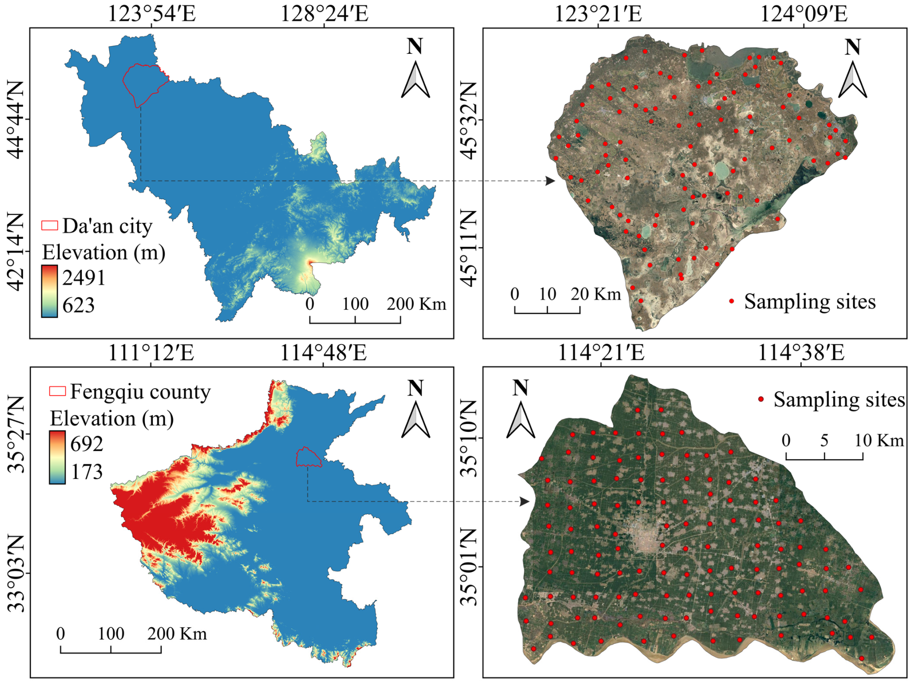
To validate the fusion performance of soil VisNIR spectra and RS imagery, this research was conducted in two contrasting agricultural regions in China: Da’an City, Jilin Province, and Fengqiu County, Henan Province (Figure 1).

Da’an City is situated in the Western Songnen Plain of Northeast China, with an area of approximately 4879 km². The topography is gently sloping, with elevations ranging from 120 to 210 m—higher in the west and lower in the east [24]. The region experiences a cold temperate continental monsoon climate, with a mean annual temperature of 4.5 °C and annual precipitation of approximately 410 mm, primarily concentrated between June and August. According to the World Reference Base for Soil Resources (WRB), the dominant soil types include Solonetz, Chernozems, and Kastanozems, which often exhibit high salinity and low organic matter content [25]. Agricultural practices primarily utilize a single-cropping system, with maize (Zea mays L.) and soybean (Glycine max L.) as the main crops. Plowing generally begins in late April or early May following the snowmelt period in recent years with increasing adoption of conservation tillage practices to enhance SOM sequestration and mitigate soil degradation. The growing season peaks between July and August, and harvest occurs in late September or early October. Therefore, in Da’an, the months from March to June represent the potential temporal window for bare soil surface detection.

Fengqiu County is located in the North China Plain and features flat alluvial terrain with elevations ranging from 45 to 110 m, covering an area of approximately 1220 km². The region has a warm temperate monsoon climate, with a mean annual temperature of 14.2 °C and average annual precipitation of 610 mm, most of which falls during the summer months of July and August. The soils—classified as Fluvisols and Cambisols under the WRB system—are derived from Yellow River alluvial deposits, supporting intensive agricultural production [26,27]. The dominant cropping system is a double-cropping rotation of winter wheat (Triticum aestivum L.) and summer maize [28]. Generally, wheat is sown in October, and maize is planted in June after the wheat harvest. The peak growing season spans July to August for maize and March to April for wheat. After the wheat harvest, substantial residues are often left on the soil surface, whereas after the maize harvest, only limited corn residues are partially retained. Therefore, compared to Da’an, Fengqiu lacks a distinct temporal window of bare soil exposure. However, the period from September to February after the maize harvest offers a more favorable window for bare soil exposure than the period following the wheat harvest.

2.2. Soil Sampling and Analysis

In Da’an, 100 topsoil samples (0–20 cm depth) were collected in 2023, while 117 samples were collected from Fengqiu in 2014. For both regions, sampling sites (Figure 1) were selected to ensure spatial representativeness while accounting for field accessibility. Non-agricultural areas such as roads and shelterbelts were avoided to minimize mixed-pixel effects in the subsequent RS analysis. Each soil sample was composited from 3–5 subsamples collected within a 5 m radius of each site. The coordinates of each sampling site were recorded using a sub-meter precision GPS device. Soil samples were transported to the laboratory, where they were air-dried, ground, and passed through a 2-mm sieve to ensure uniformity for subsequent soil spectral analysis and SOM measurement. The SOM content was determined using the potassium dichromate oxidation method [29].

2.3. VisNIR Spectra Acquisition and Processing

Soil spectral measurements were conducted using an ASD FieldSpec 4 spectrometer (Malvern Panalytical Ltd., Malvern, UK), which covers a wavelength range of 350–2500 nm with a nominal interval of 1 nm. The soil spectra in Fengqiu were sourced from Wang and Pan [30]. For the Da’an samples, measurements were taken by placing soils in a 5.6-cm diameter tray with a 75 W halogen lamp at a zenith angle of 45° in a dark room. A spectral probe with an 8° field of view was positioned vertically 18 cm above the sample. Each soil sample was rotated 90° between four sequential scans, and the average of these spectra was used as the final representative spectrum. Instrument calibration was performed every 30 min using a Spectralon reference panel.

To mitigate the impact of low signal-to-noise ratios at the spectral extremes, the wavelength regions 350–399 nm and 2401–2500 nm were excluded; consequently, only the 400–2400 nm range was used for model development. Additionally, the Savitzky–Golay smoothing algorithm with a window size of 11 and a polynomial order of 2 was applied to the measured spectra to reduce noise and enhance data quality [31]. It was conducted in the R package prospectr (version 0.2.8).

2.4. Landsat 8 Image Acquisition and Processing

Landsat 8, launched in 2013, is equipped with the Operational Land Imager and the Thermal Infrared Sensor. It provides multispectral imagery at a 30-m spatial resolution for visible, near-infrared, and shortwave infrared bands, and 100 m for thermal bands, making it suitable for monitoring soil properties. In this study, eight spectral bands were selected for analysis: the surface reflectance bands (SR_B1 to SR_B7) and the thermal band (ST_B10).

To address the limited availability of cloud-free and bare soil observations in agricultural regions, Landsat 8 imagery was composited over multiyear windows. This strategy improves spatial coverage and spectral robustness, as single-date images often provide insufficient usable data. A comprehensive compositing strategy was designed for each study area based on their distinct sampling years, climate, and cropping patterns (

Table 1. Temporal compositing strategy for Landsat 8 imagery in Da’an City and Fengqiu County.

Area	Temporal Strategy	Specific Combinations	N
Da’an	Multiyear Windows (3 to 6 years)	3-Year: 2020–2022, 2021–2023, 2022–2024 4-Year: 2019–2022, 2020–2023, 2021–2024 5-Year: 2018–2022, 2019–2023, 2020–2024 6-Year: 2017–2022, 2018–2023, 2019–2024	12
	Monthly Combinations (Mar–Jun)	1-month: Mar, Apr, May, Jun 2-month: Mar–Apr, Apr–May, May–Jun 3-month: Mar–May, Apr–Jun 4-month: Mar–Jun	10
Fengqiu	Multiyear Windows (3 to 6 years)	3-Year: 2013–2015, 2014–2016, 2015–2017 4-Year: 2013–2016, 2014–2017, 2015–2018 5-Year: 2013–2017, 2014–2018, 2015–2019 6-Year: 2013–2018, 2014–2019, 2015–2020	12
	Monthly Combinations (Sep–Feb)	1-month: Sep, Oct, Nov, Dec, Jan, Feb 2-month: Sep–Oct, Oct–Nov, Nov–Dec, Dec–Jan, Jan–Feb 3-month: Sep–Nov, Oct–Dec, Nov–Jan, Dec–Feb 4-month: Sep–Dec, Oct–Jan, Nov–Feb 5-month: Sep–Jan, Oct–Feb 6-month: Sep–Feb	21

Note: N represents the combination number under each temporal strategy.

). The strategy involved creating multiyear composites for different rolling time windows (e.g., 3-year, 4-year) and testing various monthly combinations within the critical agricultural periods for each region to identify the optimal temporal window for bare soil exposure. The agricultural systems differed significantly: Da’an utilized a single-cropping system, whereas Fengqiu practiced double-cropping. Consequently, a wider range of monthly combinations was evaluated in Fengqiu (n = 21) than in Da’an (n = 10) to retrieve soil spectral information from RS imagery. The total number of unique year–month combinations was 252 for Fengqiu and 120 for Da’an.

To ensure image quality, the pixels contaminated by clouds and cloud shadows were masked. Median compositing was then applied to the remaining clear-sky pixels from all images within each specified temporal combination to generate cloud-free composites for subsequent analysis. All image processing was conducted on the Google Earth Engine (GEE) platform, which provides efficient access to the data archive and robust geospatial analysis tools [9,10].

2.5. The Fusion Method

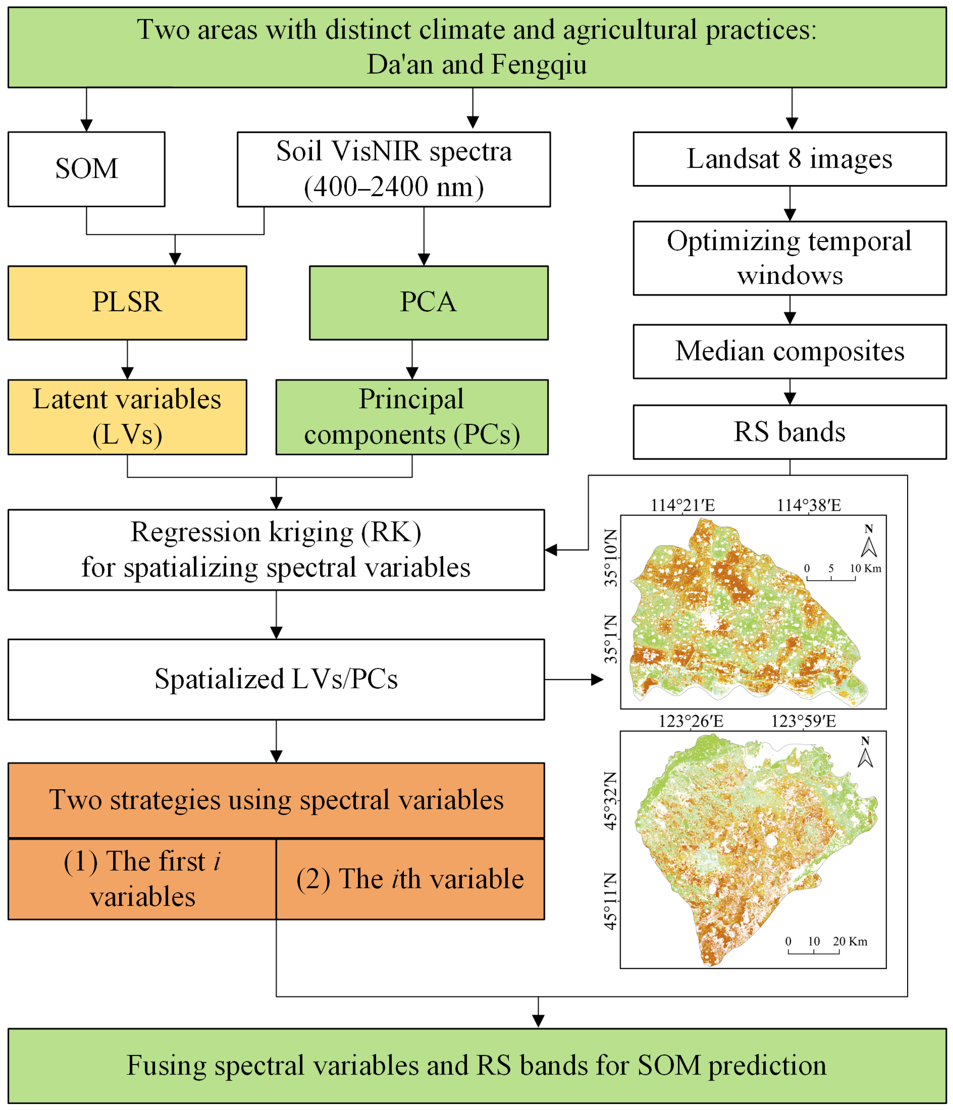
This study proposes a novel method of fusing soil VisNIR spectra and RS bands to predict SOM (Figure 2). The procedure consists of three main steps:

Step 1: Extraction of spectral variables from the soil VisNIR spectra. We employed a supervised method, PLSR, to extract spectral variables (i.e., latent variables, LVs), which might have strong correlations with SOM. In this study, the number of LVs was determined arbitrarily by a threshold of 70% for the cumulative variance in SOM explained by the spectra. Furthermore, PCA—a commonly used technique for extracting spectral variables (i.e., PCs) in the literature—was employed as a benchmark to evaluate the performance of PLSR. An equivalent number of PCs and LVs were extracted for a direct comparison.

Step 2: Spatialization of PCs and LVs using RK. For each PC or LV, we first used a random forest (RF) model based on composites of multitemporal Landsat 8 images to obtain the spatial trend. Then, the residuals from the RF model were interpolated using OK based on their spatial autocorrelation. The final spatialized map for each LV or PC was generated by summing the predicted trend surface and the kriged residual map.

Step 3: Establishing fusion models by integrating PCs/LVs and RS bands. We implemented two fusion strategies. The first involved combining the first i PCs/LVs with the RS bands. The second involved selectively combining individual PCs/LVs (ith PC/LV) with the RS bands. This strategy was motivated by the fact that not all PCs/LVs have a strong relationship with SOM.

2.6. Model Calibration and Evaluation

Random forest was selected to calibrate the two types of relationships: (1) between PCs/LVs and RS bands, and (2) between SOM and the combined set of RS bands and PCs/LVs. As an ensemble machine learning algorithm, RF constructs multiple decision trees and aggregates predictions through voting or averaging to increase model accuracy and stability. RF has been successfully and widely used to map soil properties in the literature. In this study, the number of trees was tested using the values 500 and 1000, and the node size was tested from 1 to 10. The number of variables available for splitting at each node (mtry) was tested across all possible integer values from one to the total number of input variables. All these parameters were optimized simultaneously using a grid search approach with cross-validation.

A 10-fold cross-validation approach was employed to evaluate the prediction accuracy. The evaluation metrics included R² and RMSE:

$${\mathrm{R}}^2=1-{\displaystyle \frac{{\sum }_{i=1}^n{\left(y_i-{\widehat{y}}_i\right)}^2}{{\sum }_{i=1}^n{\left(y_i-\overline{y}\right)}^2}}\hspace{1em}$$

(1)

$$\mathrm{R}\mathrm{M}\mathrm{S}\mathrm{E}=\sqrt{{\displaystyle \frac{1}{n}}\sum _{i=1}^n{\left(y_i-{\widehat{y}}_i\right)}^2}\hspace{1em}$$

(2)

where $y_i$ and ${\widehat{y}}_i$ are the observed and predicted SOM values, respectively, $\overline{y}$ is the mean of the observed values, and n is the number of samples. A higher R² and a lower RMSE indicate better predictive performance of the model for SOM.

3. Results

3.1. Statistics of SOM Contents

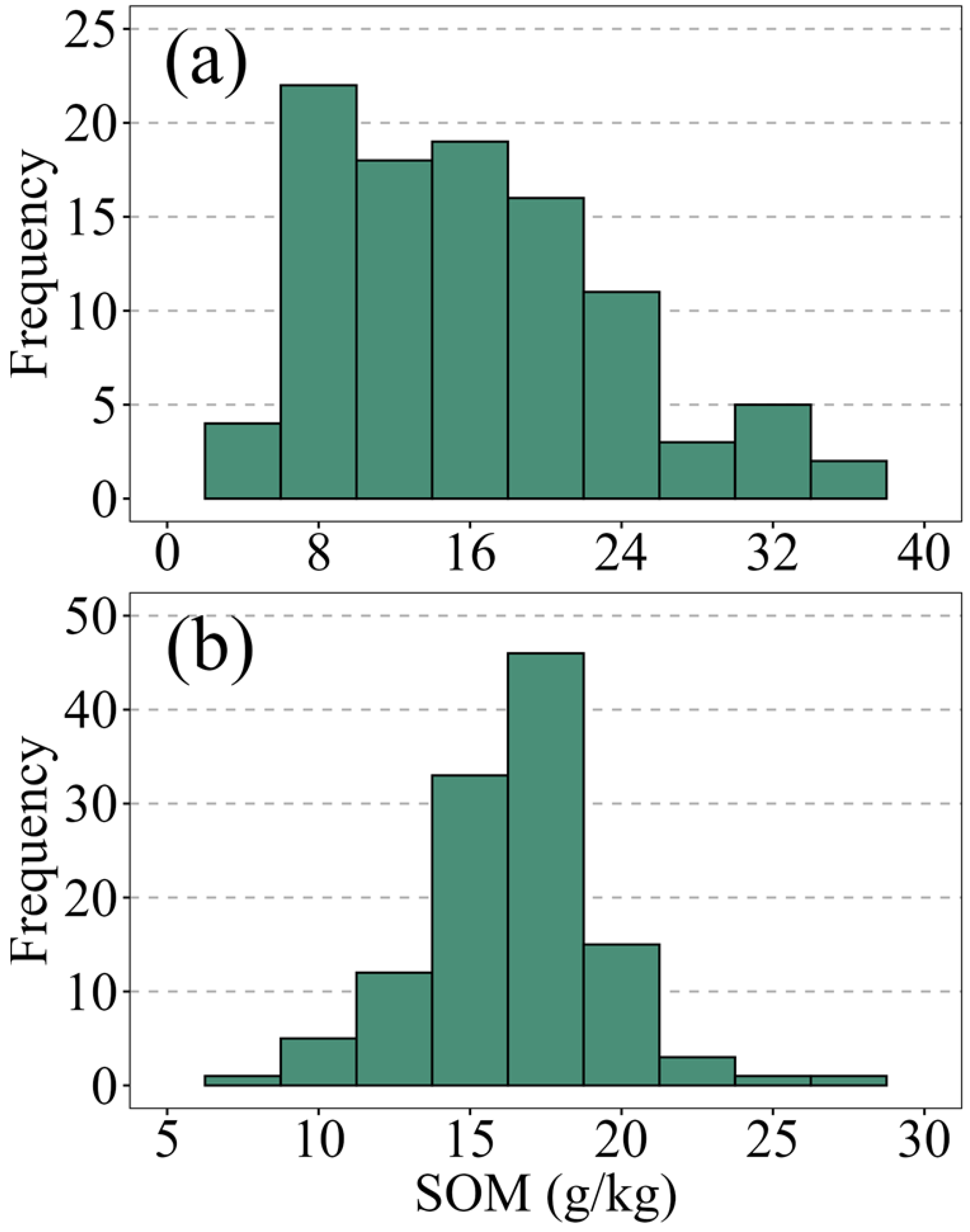
The mean SOM content was 16.21 and 16.40 g/kg for Da’an and Fengqiu, respectively. Despite similar means in these two regions, the SOM content in Da’an exhibited greater variability, ranging from 4.34 to 36.00 g/kg and standard deviation (SD) with 7.40 g/kg, compared to Fengqiu’s range of 8.60 to 28.40 g/kg (SD = 3.01 g/kg). This difference in variability was quantified by the coefficient of variation (CV), which was 45.66% for Da’an (indicating moderate variability) and 18.36% for Fengqiu (indicating low variability), as classified by [32]. The skewness values for Da’an (0.65) and Fengqiu (0.41) indicated that the SOM values for both regions were approximately normally distributed; consequently, no data transformation was applied prior to modeling (Figure 3).

3.2. Extracting Spectral Variables from VisNIR Spectra

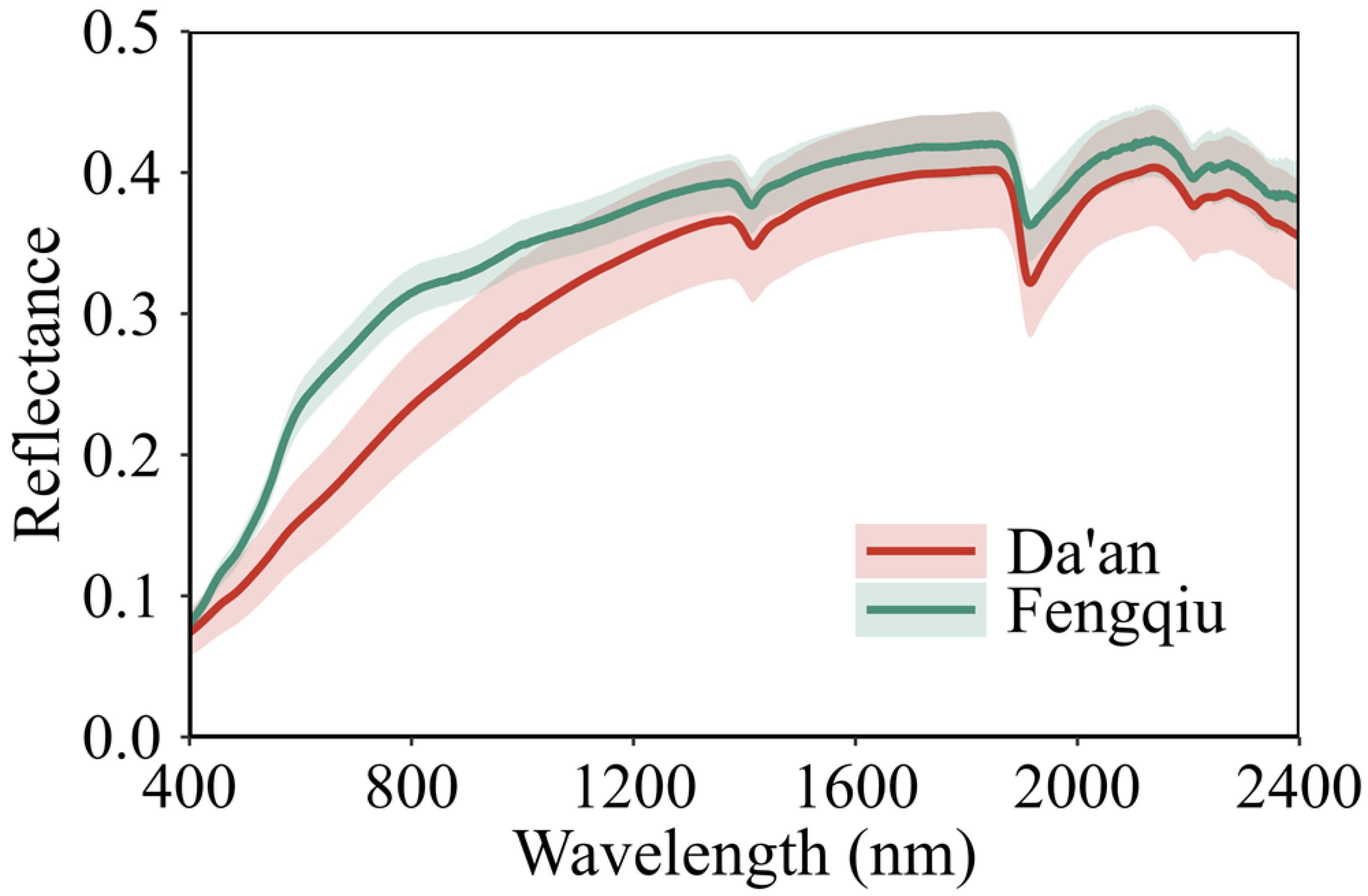
Soils from Da’an demonstrated lower reflectance compared to those from Fengqiu, particularly in the visible region (400–780 nm, Figure 4) where SOM and iron oxides strongly absorb radiation. The greater variability was demonstrated in soil spectra in Da’an, probably resulting from its higher heterogeneity of soil properties (e.g., SOM content). In contrast, Fengqiu’s spectra showed higher overall reflectance with less variability.

We employed both PLSR and PCA to extract spectral variables for subsequent fusion with RS bands. For Da’an, the first six LVs derived from PLSR collectively explained 70.64% of the variance in SOM, with individual contributions of LV1 to LV6 being 30.77%, 10.69%, 9.91%, 3.89%, 2.23%, and 13.15%, respectively. These same LVs accounted for 99.97% of the variance in the soil spectra. For Fengqiu, the first five LVs explained 74.08% of the variance in SOM, with respective contributions of 20.03%, 5.49%, 16.04%, 23.06%, and 9.46% for LV1 to LV5, while capturing 99.94% of the spectral variance. For comparison, an equivalent number of PCs were extracted using PCA. The first six PCs explained 99.98% variance of soil spectra for Da’an, while the first five PCs explained 99.95% variance of soil spectra for Fengqiu.

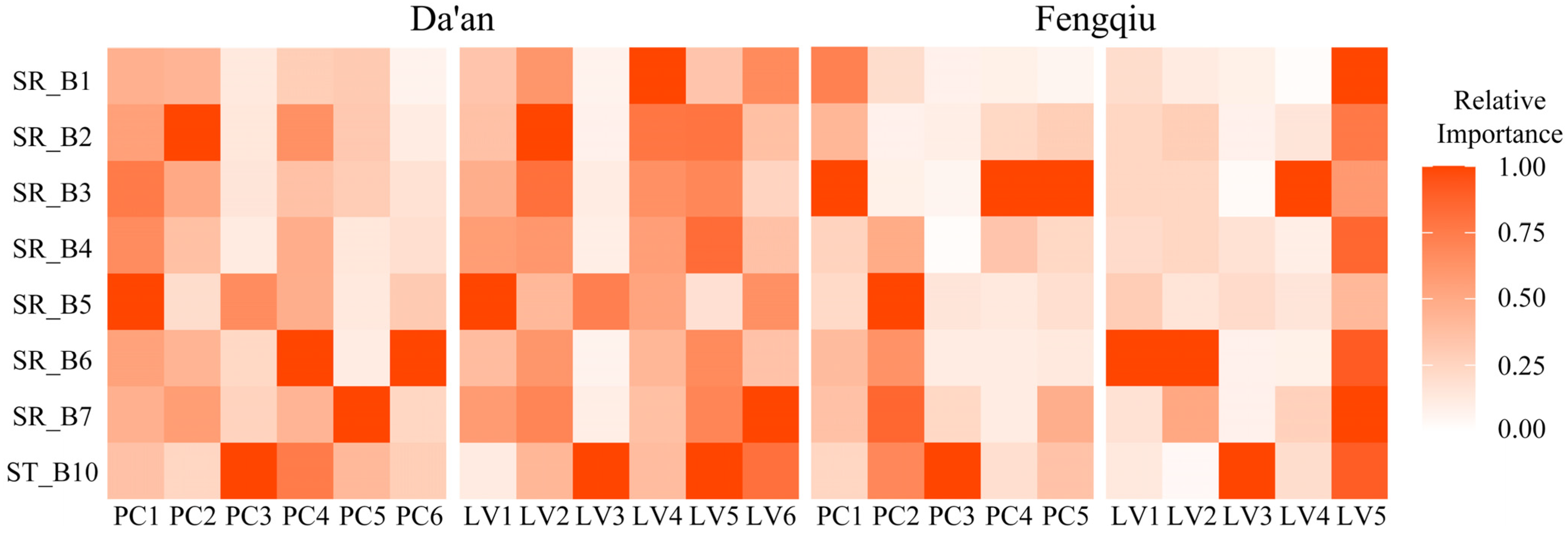
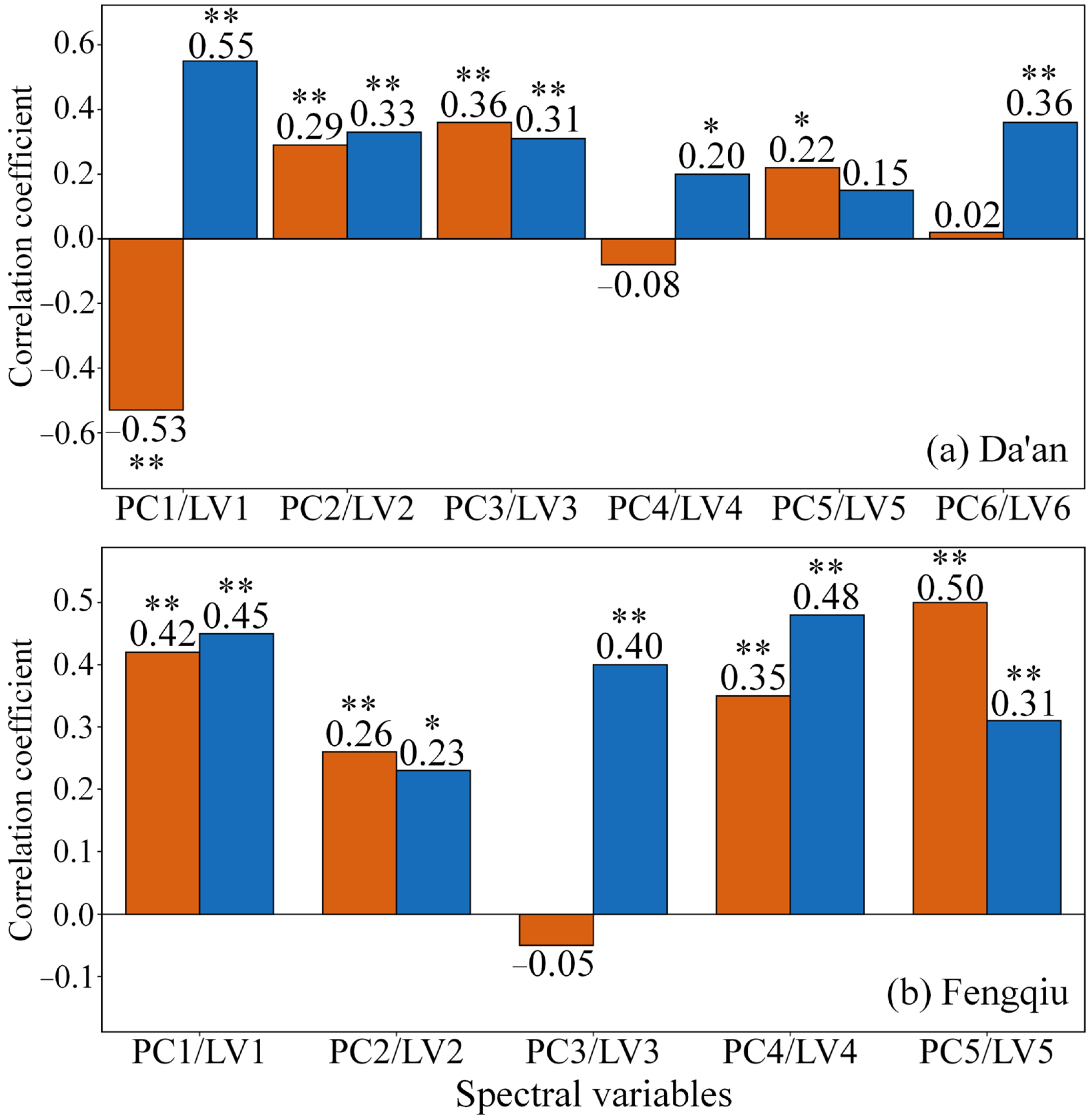
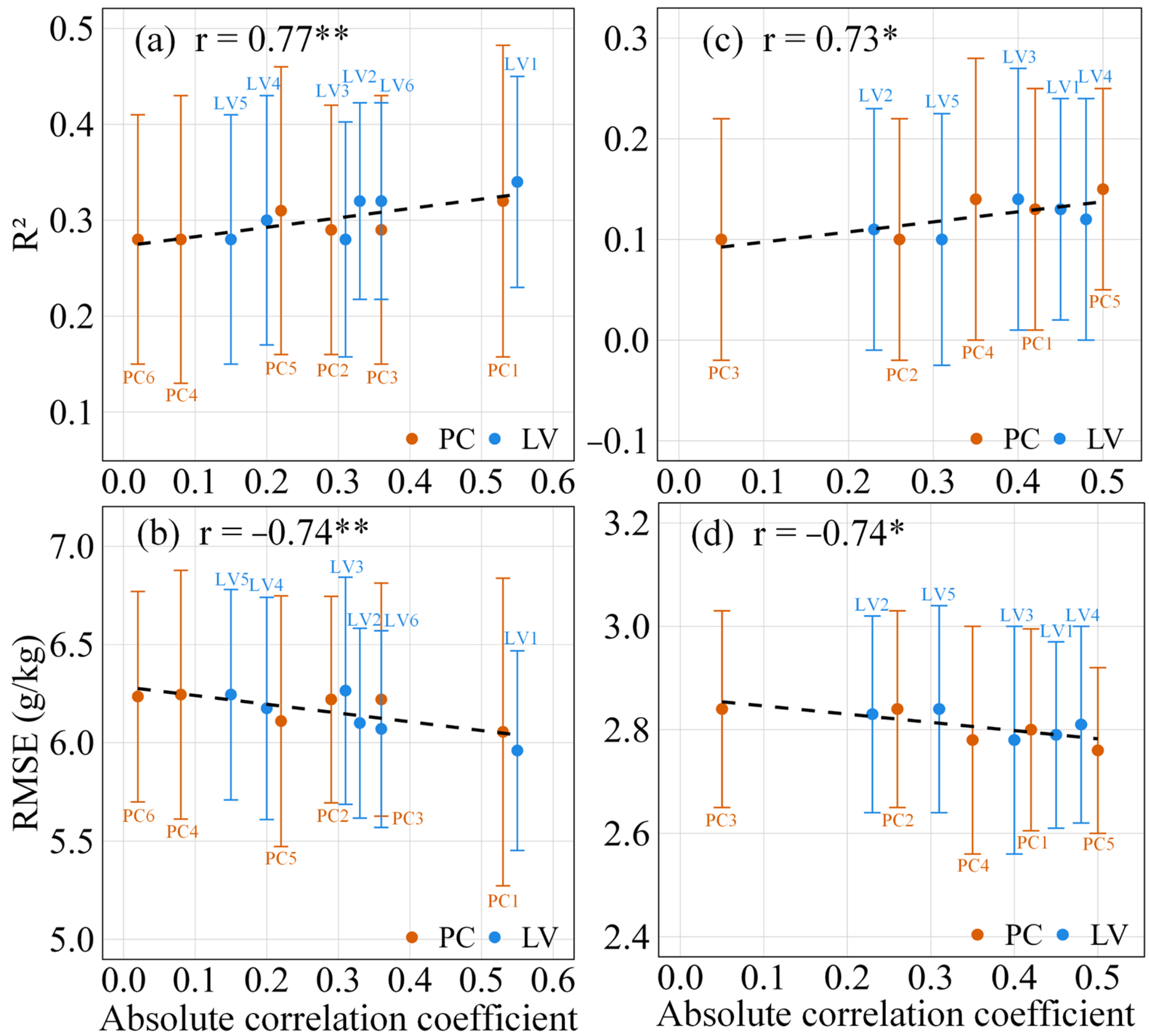
The correlations between PCs/LVs with SOM are presented in Figure 5. For Da’an, both PC1 and LV1 showed the strongest correlations with SOM (r = −0.53 and r = 0.55, respectively). While the correlations of subsequent LVs generally decreased with component order, LV6 showed an increased correlation (r = 0.36). A similar pattern was observed for PCs, with PC1, PC2, PC3, and PC5 following comparable trends to LVs. However, PC4 (r = −0.08) and PC6 (r = 0.02) demonstrated substantially weaker correlations compared to LV4 (r = 0.20) and LV6 (r = 0.36). In Fengqiu, LV1, LV3, and LV4 exhibited relatively strong and consistent correlations with SOM (ranging from 0.40 to 0.48), while LV5 showed a moderate correlation (r = 0.31) and LV2 demonstrated the weakest relationship (r = 0.23). The correlation patterns for PCs differed notably from LVs: while PC1 and PC2 showed similar correlations to LVs, PC3 (r = −0.05) and PC4 (r = 0.35) were substantially lower than LV3 (r = 0.40) and LV4 (r = 0.48). Interestingly, PC5 (r = 0.50) exceeded the correlation of LV5 (r = 0.31).

3.3. Spatialization of PCs and LVs

The spatialization of PCs and LVs was performed using RK, which was tested based on all composite images with unique year–month combinations (Table 1). For comparison, we applied OK for spatializing PCs and LVs, which was commonly used in the literature.

Table 2. Spatialization accuracy (R²) of principal components (PCs) and latent variables (LVs) by ordinary kriging (OK) and residual kriging (RK).

Area	Method	PC1/LV1	PC2/LV2	PC3/LV3	PC4/LV4	PC5/LV5	PC6/LV6
Da’an	OK	0.14/0.14	0.18/0.21	−0.03/−0.01	0.18/0.24	0.13/0.14	0.03/−0.21
	RK	0.36/0.33	0.47/0.50	0.44/0.44	0.27/0.26	0.35/0.23	0.17/0.06
Fengqiu	OK	0.09/0.05	0.32/0.39	0.40/0.47	0.27/0.15	0.17/0.17	No data
	RK	0.18/0.23	0.52/0.54	0.48/0.45	0.41/0.37	0.36/0.31	No data

presents the optimal results selected from all of the year–month combinations based cross-validation performance. The results show that RK consistently yielded higher spatialization accuracy than OK in both areas. Substantial improvements were observed particularly for intermediate PCs/LVs: in Da’an, the R² values for PC2/LV2 increased from 0.18/0.21 with OK to 0.47/0.50 with RK, while PC3/LV3 showed remarkable improvement from −0.03/−0.01 to 0.44/0.44. Similarly, in Fengqiu, the R² for PC2/LV2 increased from 0.32/0.39 to 0.52/0.54.

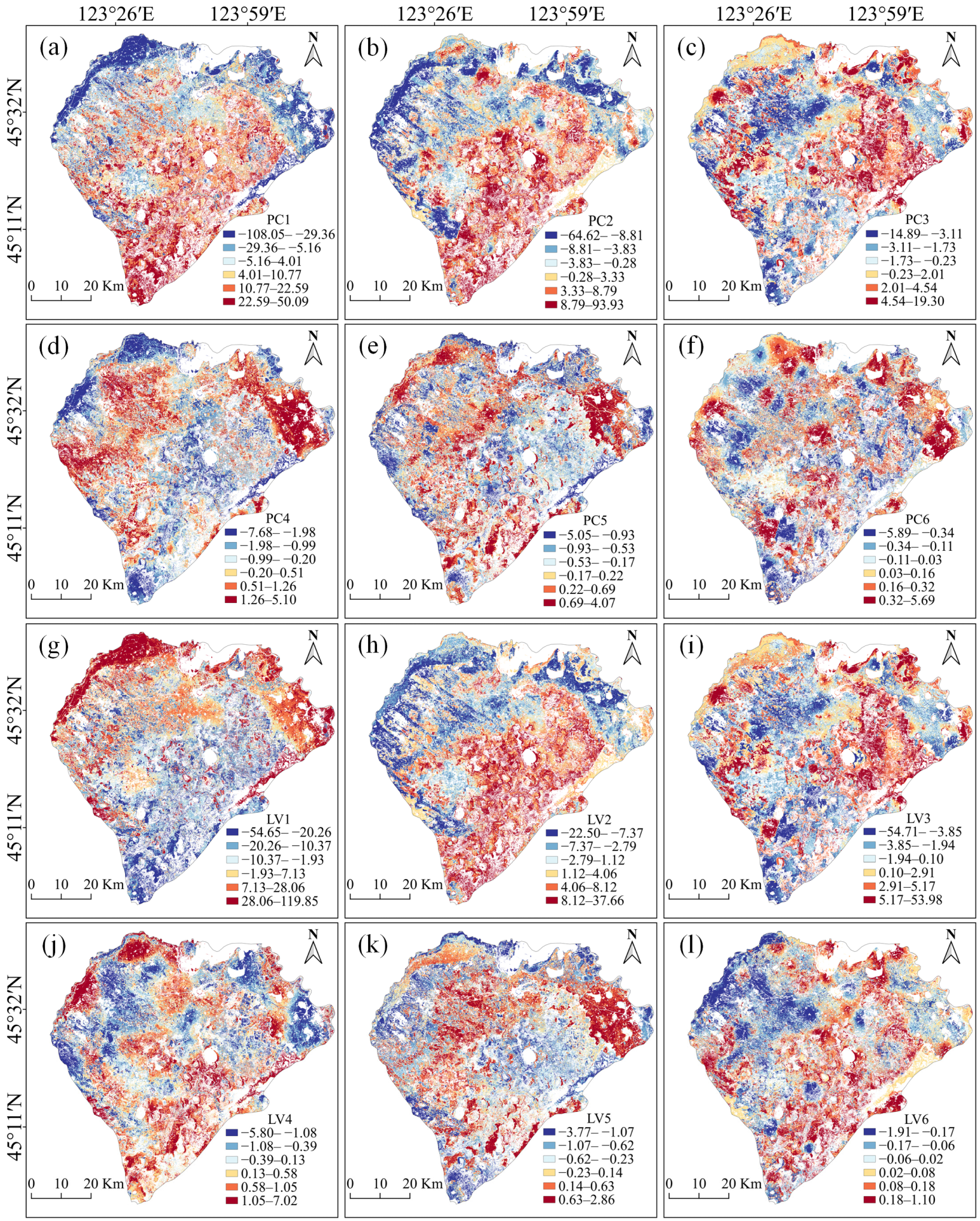
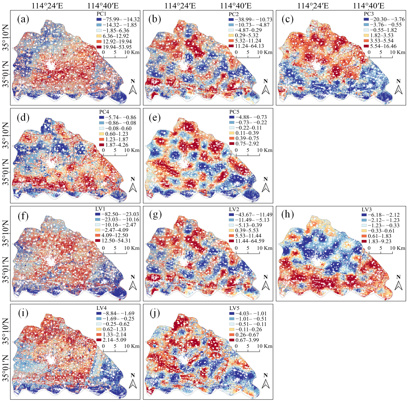
Despite these overall improvements, certain PC/LV maintained relatively low spatialization accuracy even with RK. Specifically, PC6/LV6 in Da’an achieved R² values of 0.17/0.06, and PC1/LV1 in Fengqiu remained low at 0.18/0.23. Notably, PC1/LV1, despite exhibiting the strongest correlation with SOM content, showed limited spatialization accuracy, with R² values improving from 0.14/0.14 to 0.36/0.33 in Da’an and from 0.09/0.05 to 0.18/0.23 in Fengqiu. These limitations may consequently affect the performance of subsequent fusion models. The maps of all PCs and LVs for both areas are presented in Figure A1 and Figure A2.

3.4. SOM Predictions Using the Fusion Method

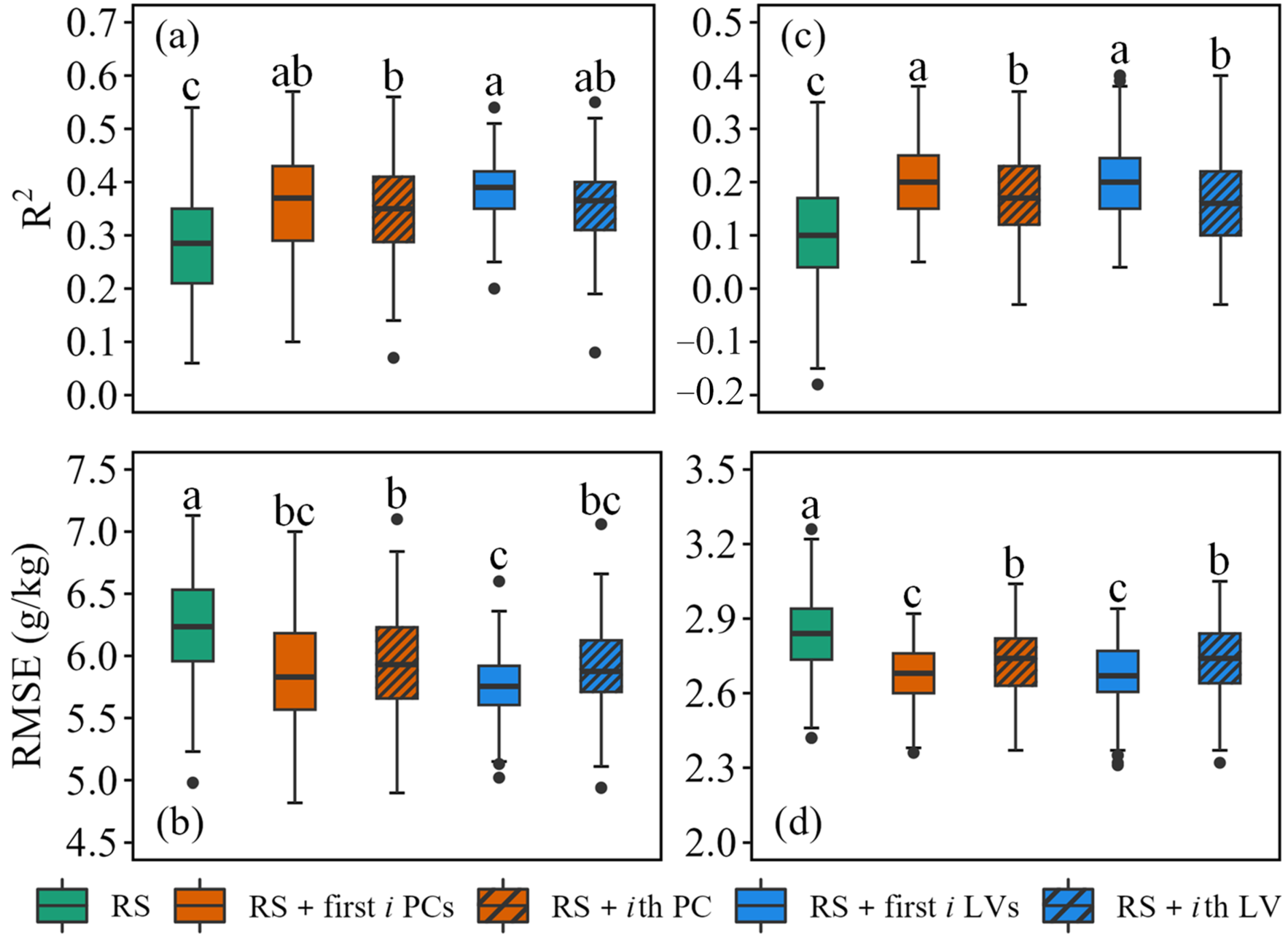
We evaluated two fusion strategies (four variants), i.e., RS + first i PCs/LVs and RS + ith PC/LV (i = 6 for Da’an and = 5 for Fengqiu). For each multiyear window, the optimal spatialization of PCs/LVs selected among all available monthly combinations were fused with their corresponding RS composite images across all unique year–month combinations (Table 1). The significance of differences in mean R² and RMSE between the RS method (using RS bands alone) and the four fusion variants was assessed using one-way ANOVA with post-hoc tests at a 5% significance level. The results are presented in Figure 6 and

Table 3. The prediction accuracy of SOM for the remote sensing (RS) method and the four variants of the fusion method.

Area	Metrics	Method	Mean	Median	Min	Max	SD
Da’an	R2	RS	0.28	0.29	0.06	0.54	0.09
		RS + first i PCs	0.37	0.37	0.10	0.57	0.09
		RS + ith PC	0.34	0.35	0.07	0.56	0.09
		RS + first i LVs	0.39	0.39	0.20	0.54	0.06
		RS + ith LV	0.36	0.37	0.08	0.55	0.08
	RMSE (g/kg)	RS	6.23	6.24	4.98	7.13	0.41
		RS + first i PCs	5.85	5.83	4.82	7.00	0.42
		RS + ith PC	5.95	5.93	4.90	7.10	0.41
		RS + first i LVs	5.76	5.76	5.02	6.60	0.28
		RS + ith LV	5.89	5.88	4.94	7.06	0.35
Fengqiu	R2	RS	0.10	0.10	−0.18	0.35	0.10
		RS + first i PCs	0.21	0.20	0.05	0.38	0.07
		RS + ith PC	0.17	0.17	−0.03	0.37	0.08
		RS + first i LVs	0.20	0.20	0.04	0.40	0.08
		RS + ith LV	0.17	0.16	−0.03	0.40	0.09
	RMSE (g/kg)	RS	2.84	2.84	2.42	3.26	0.15
		RS + first i PCs	2.67	2.68	2.36	2.92	0.11
		RS + ith PC	2.73	2.74	2.37	3.04	0.14
		RS + first i LVs	2.67	2.67	2.31	2.94	0.13
		RS + ith LV	2.72	2.74	2.32	3.05	0.14

Note: RS, PC, and LV indicate remote sensing, principal component, and latent variable, respectively. RS + first i PCs, RS + ith PC, RS + first i LVs, and RS + ith LV are four fusion variants.

.

In Da’an, both fusion strategies significantly improved the prediction performance of SOM compared to the RS method (mean R² = 0.28, RMSE = 6.23 g/kg). The RS + first i LVs method achieved the highest accuracy, with a mean R² of 0.39 and RMSE of 5.76 g/kg, representing a 39.3% improvement in R² and a 7.5% reduction in RMSE. This was closely followed by RS + first i PCs (mean R² = 0.37, and RMSE = 5.85 g/kg). Among the results of four fusion variants—RS + first i PCs, RS + ith PC, RS + first i LVs, and RS + ith LV, statistical analysis indicated that RS + first i LVs significantly outperformed RS + ith PC (p < 0.05), though no other pairwise differences reached significance. However, LV-based methods demonstrated greater predictive stability than PC-based methods, as reflected by lower SD in both R² and RMSE values (Table 3).

In Fengqiu, the fusion method also enhanced the prediction accuracy of SOM compared to the RS method (mean R² = 0.10, and RMSE = 2.84 g/kg), though the improvements were more modest than those observed in Da’an. The RS + first i PCs method yielded the highest mean R² (0.21) and lowest RMSE (2.67 g/kg), representing a 110% improvement in R² and a 6.0% reduction in RMSE. The RS + first i LVs method performed similarly (mean R² = 0.20, and RMSE = 2.67 g/kg). No significant differences were observed between RS + first i PCs and RS + first i LVs or between RS + ith PC and RS + ith LV, while the RS + first i PCs method was better than the RS + ith PC method and the RS + first i LVs method outperformed the RS + ith LV method. Meanwhile, the fusion strategy employing multiple variables (first i PCs/LVs) consistently outperformed that using a single variable (ith PC/LV), highlighting the importance of incorporating comprehensive spectral information for SOM prediction in this region. It should be noted that the SD of R² and RMSE for LV-based methods were similar to that for PC-based methods.

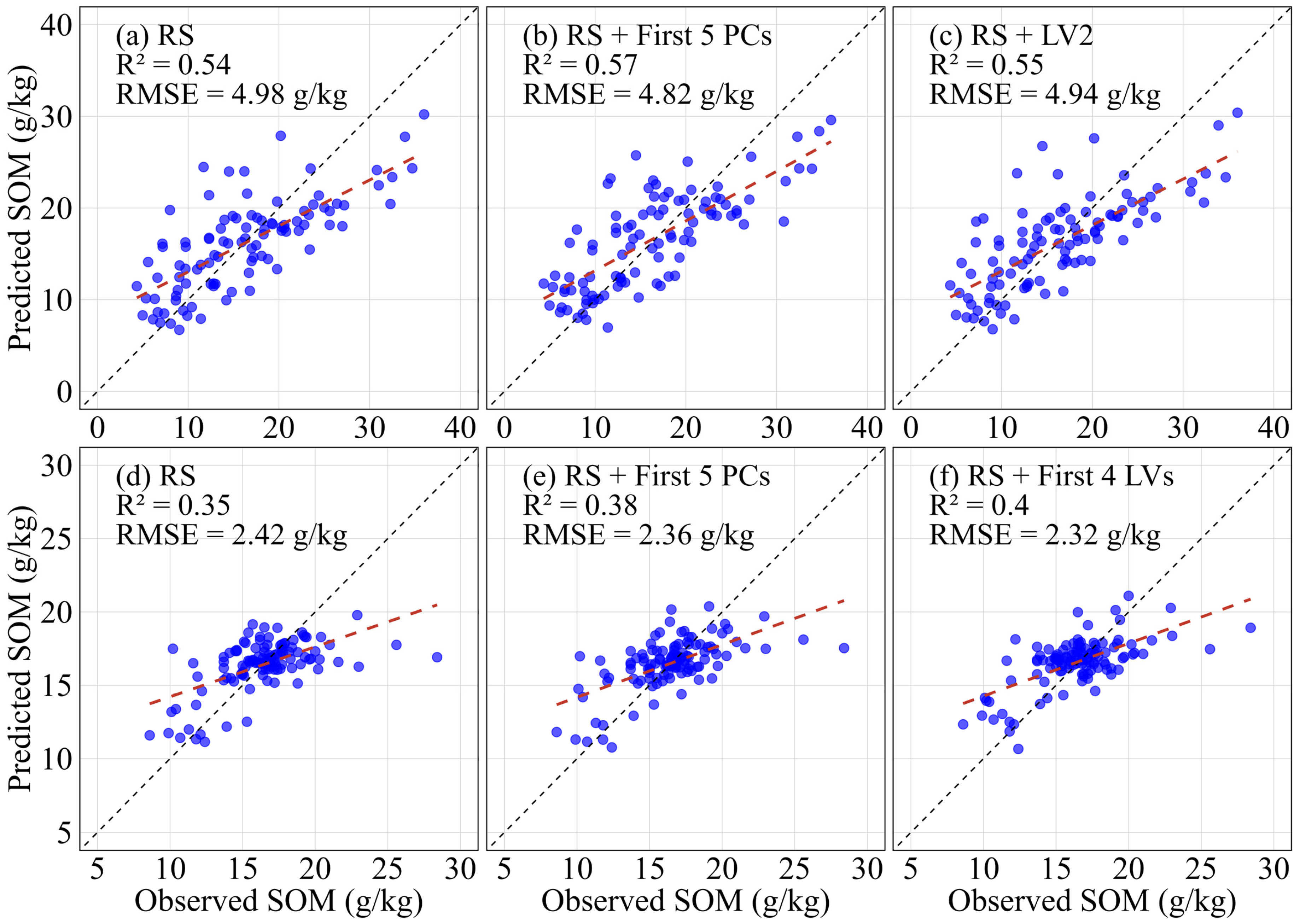
For both study areas, the fusion method achieved substantially higher peak performance compared to the RS method (Table 3). The RS + first i PCs method yielded the most substantial improvement, reaching a maximum R² of 0.57 and minimum RMSE of 4.82 g/kg, indicating a 5.6% increase in predictive accuracy and a 3.2% reduction in error compared to the best result of the RS method (R² = 0.54, and RMSE = 4.98 g/kg). The LV-based fusion method (RS + ith LV) also demonstrated strong performance with maximum R² of 0.55 and minimum RMSE of 4.94 g/kg. In Fengqiu, both RS + first i LVs and RS + ith LV achieved the highest R² value of 0.40, representing a 14.3% improvement over the maximum R² of 0.35 for the RS method. In addition, the RS + first i LVs method produced the smallest RMSE (2.31 g/kg), a 4.5% reduction from the RS method’s minimum of 2.42 g/kg. These improvements are visually corroborated by the scatter plots in Figure 7, which shows reduced dispersion and tighter clustering along the 1:1 line for fusion-based predictions compared to the results of the RS method. Therefore, these results demonstrate that the fusion method not only improves average accuracy but also enhances the best-case predictive performance across temporal combinations.

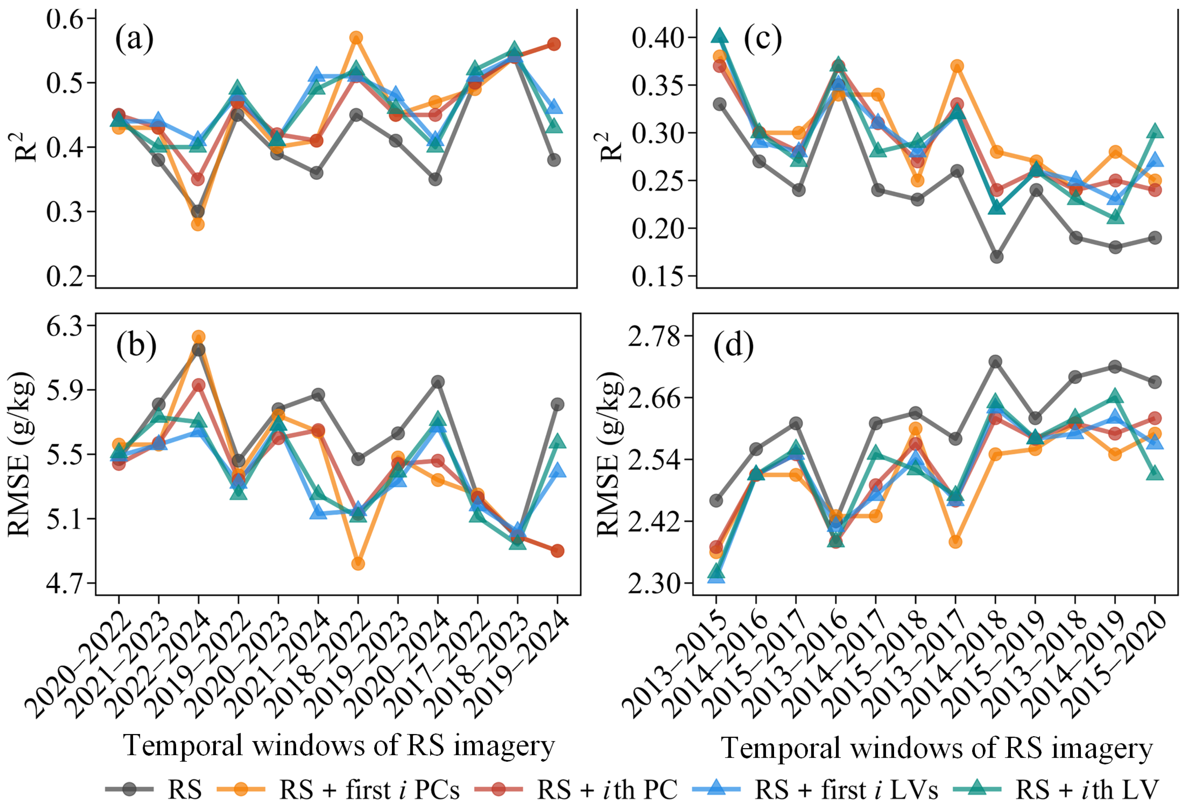
3.5. Temporal Stability of Fusion Method

We further investigated the temporal stability of the fusion method’s performance across different multiyear windows, a critical consideration for scenarios where RS imagery availability may be limited in certain years. For each window, the optimal SOM prediction results from all available monthly combinations are shown for the RS method and the fusion method with four variants (RS + first i PCs, RS + ith PC, RS + first i LVs, and RS + ith LV) in Figure 8. The results, in terms of R² and RMSE, clearly demonstrate that the fusion method consistently enhanced prediction accuracy compared to the RS method in both Da’an and Fengqiu.

In Da’an, the RS method showed moderate but variable performance with a mean R² of 0.41 (range: 0.30–0.54) and a mean RMSE of 5.63 g/kg (range: 4.98–6.15 g/kg). Both PC-based fusion methods significantly improved predictive accuracy, compared to the RS method. The RS + first i PCs method achieved a higher mean R² of 0.46 (range: 0.28–0.57) and a lower mean RMSE of 5.41 g/kg (range: 4.82–6.23 g/kg). Notably, it achieved the highest performance in the 2018–2022 window (R² = 0.57, and RMSE = 4.82 g/kg). Similarly, the RS + ith PC method yielded a mean R² of 0.46 (range: 0.35–0.56) and a mean RMSE of 5.39 g/kg (range: 4.90–5.93 g/kg), with peak performance in the 2019–2024 window (R² = 0.56, and RMSE = 4.90 g/kg). The LV-based fusion methods also enhanced predictions and exhibited greater temporal stability. The RS + first i LVs method produced a mean R² of 0.47 (range: 0.41–0.54) and a mean RMSE of 5.38 g/kg (range: 5.02–5.68 g/kg), with the best performance in the 2018–2023 window (R² = 0.54, and RMSE = 5.02 g/kg). The RS + ith LV method resulted in a mean R² of 0.46 (range: 0.40–0.55) and a mean RMSE of 5.41 g/kg (range: 4.94–5.73 g/kg), peaking in the 2018–2023 window (R² = 0.55, and RMSE = 4.94 g/kg). The lower variability of R² and RMSE for LV-based methods (e.g., SD of R² = 0.04 for RS + first i LVs) confirm their superior stability across years compared to PC-based and RS methods.

In Fengqiu, the RS method performed poorly and inconsistently across multiyear windows, with a mean R² of 0.24 (range: 0.17–0.35) and a mean RMSE of 2.61 g/kg (range: 2.42–2.73 g/kg). All fusion variants substantially improved accuracy. The PC-based fusion methods increased the mean R² to 0.30 (RS + first i PCs; range: 0.24–0.38) and 0.29 (RS + ith PC; range: 0.24–0.37), while reducing the mean RMSE to 2.51 g/kg (range: 2.36–2.61 g/kg) and 2.53 g/kg (range: 2.37–2.62 g/kg), respectively. The RS + first i PCs method achieved the highest R² (0.38) and the lowest RMSE (2.36 g/kg) in the 2013–2015 window, and the RS + ith PC method achieved a mean R² (0.37) and RMSE (2.37 g/kg) in the same window. The LV-based fusion methods also showed notable improvements. The RS + first i LVs method attained a mean R² of 0.29 (range: 0.22–0.40) and a mean RMSE of 2.52 g/kg (range: 2.31–2.64 g/kg), with optimal performance in the 2013–2015 window (R² = 0.40, and RMSE = 2.31 g/kg). The RS + ith LV method achieved a mean R² of 0.29 (range: 0.21–0.40) and a mean RMSE of 2.53 g/kg (range: 2.32–2.66 g/kg), excelling in the 2013–2015 window (R² = 0.40, and RMSE = 2.32 g/kg).

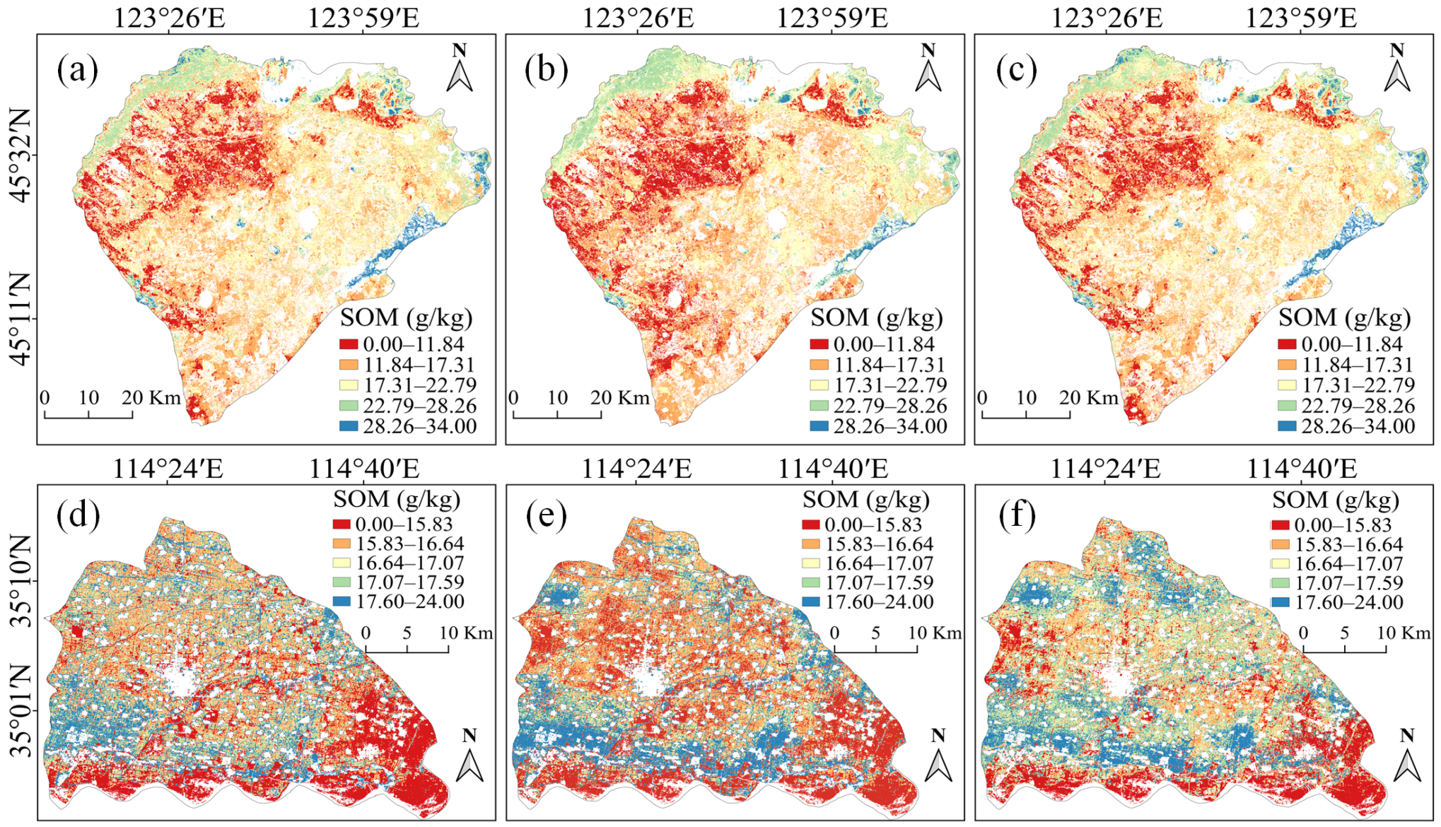
3.6. SOM Distributions in Two Areas

The SOM maps in Da’an and Fengqiu (Figure 9) were generated by the optimal models of the RS method, the RS + PC method, and the RS + LV method. These models were selected through 10-fold cross-validation across all temporal combinations based on the highest validation R² and low RMSE values. Their corresponding RF parameters are listed in

Table A1. Optimal Random Forest parameters for the SOM predictions in Figure 7 and Figure 9.

Area	Model	ntree	Nodesize	mtry
Da’an	RS	1000	3	8
	RS + First 5 PCs	500	1	13
	RS + LV2	1000	2	6
Fengqiu	RS	500	8	1
	RS + First 5 PCs	500	6	5
	RS + First 4 LVs	1000	3	4

. In Da’an, overall, all methods consistently revealed a distinct east-high, west-low pattern in SOM (Figure 9a–c). This pattern is primarily driven by land use. High salinity in the Western areas led to lower SOM. In contrast, the central parts show moderately higher SOM content due to cultivation. The highest SOM values are consistently predicted along the northwestern and eastern boundaries, which were mainly characterized by high-quality drylands and paddy fields, respectively. Compared to the RS method, the RS + PC fusion result exhibits a larger spatial extent of low-value SOM patches in the mid-Western and Southwestern regions. The RS + LV fusion method shows a slight expansion in the range of high-value regions, particularly evident along the Northern and Eastern boundaries. This enhancement might better capture the expected high SOM in the paddy fields.

In Fengqiu, the resulting maps show a similar spatial pattern of SOM across the different methods. The high SOM values are predominantly located in the Northeastern and south–central sectors of the county (Figure 9d–f). This pattern can be attributed to agricultural practices and proximity to branches of the Yellow River. Conversely, the lowest SOM values are found along the Yellow River in the south and southeastern areas. These areas can be affected by river flooding. Compared to the RS method, the RS + PC result sharpens the spatial contrasts. It shows an expanded area of low-value SOM in the central–northern region. The RS + LV method shows noticeably higher SOM levels in the Central and Northern regions. The spatial extent of the low-value area in the mid-western region is intermediate between those predicted by the RS method and the RS + PC method, suggesting a more balanced and potentially more accurate representation of the spatial distribution.

4. Discussion

4.1. Importance of Spectral Feature Extraction in VisNIR Data for Fusion with RS

A key limitation laboratory of VisNIR spectroscopy is its restriction to point-based predictions, while RS imagery provides continuous spatial coverage [33]. To bridge this gap, data fusion approaches are commonly employed to integrate the complementary strengths of both techniques. In this study, all four fusion variants (RS + first i PCs, RS + first i LVs, RS + ith PC, and RS + ith LV) significantly improved SOM prediction accuracy in both Da’an and Fengqiu. This aligns with previous findings that integrating VisNIR spectra and RS imagery enhances SOM prediction compared to using RS data alone [18,20]. Specifically, in terms of mean values of R² and RMSE derived from 120 composited images (Table 1), R² improved from 0.28 (RS alone) to 0.34–0.39 (fusion methods), and RMSE decreased from 6.23 g/kg to 5.76–5.93 g/kg (Table 3) in Da’an. Similar improvements were observed in Fengqiu, where the fusion method boosted the mean R² from 0.10 to 0.17–0.21 and lowered RMSE from 2.84 g/kg to 2.67–2.73 g/kg. These consistent improvements confirm the advantage of the fusion method over using RS alone.

Crucially, our results further revealed that the variable extraction method of soil spectra influences prediction accuracy of SOM by the fusion method. In Da’an, the LV-based fusion methods achieved more stable predictive accuracy than those based on PC-based methods. Although fusion consistently outperformed RS alone, many existing studies overlooked the relationship between extracted VisNIR variables and target soil properties. For example, Xu, et al. [20] reported that in a region with similar soils to Fengqiu, fusing PCs with RS imagery improved prediction, with R² increasing from 0.53 to 0.72; however, among the first four PCs (from field soil spectra in 400–2450 nm) used in their fusion model with GF-1 imagery, only PC1 and PC3 strongly impacted SOM prediction. In addition, Rossel and Chen [21] demonstrated that PCs from VisNIR spectra captured different soil properties; some were related to iron oxides or clay content, while only a subset correlated with organic carbon. This pattern underscores that PCA, as an unsupervised method, maximizes spectral variance rather than its covariance with specific soil properties, which can result in components with little relevance to SOM. This issue was also evident in our study (Figure 5), where PC4 and PC6 in Da’an and PC3 in Fengqiu showed near-zero correlation with SOM. Therefore, selecting PCs based solely on the proportion of spectral variance explained (e.g., 99%) risks including these irrelevant components, potentially reducing SOM prediction accuracy.

In contrast, PLSR, a supervised method, explicitly incorporates the target variable during spectral feature extraction by maximizing the covariance between soil spectra and properties [34]. Consequently, the resulting LVs not only capture spectral variation but also maintain a stable relationship with SOM, effectively avoiding variables with negligible predictive power. This methodological advantage is confirmed by our findings: while some PCs and LVs showed comparable correlations with SOM (e.g., PC1 and LV1), the LVs consistently avoided the near-zero correlations observed for certain PCs (e.g., PC4 with r = −0.08 and PC6 with r = 0.02 in Da’an, PC3 with r = −0.05 in Fengqiu). Furthermore, the accuracy (R² and RMSE) of the RS + ith PC/LV method was significantly correlated with the absolute correlation between each PC/LV and SOM (p < 0.01 in Da’an; p < 0.05 in Fengqiu; Figure 10). This indicates that components with stronger SOM correlations lead to higher predictive accuracy in the fusion method. Consequently, the LV-based fusion methods delivered more stable performance. In Da’an, the RS + first i LVs method achieved the highest mean R² (0.39), the lowest RMSE (5.76 g/kg), and lower variability across different composited images with various year–month combinations than the PC-based methods (Table 3). In Fengqiu, the LV-based and PC-based methods demonstrated comparable performance.

Moreover, the temporal stability of the fusion method across multiyear windows provides further evidence for the advantage of supervised extraction of spectral variables from soil spectra (Figure 8). In Da’an, while the RS + first i PCs method reached a peak R² of 0.57 in the 2018–2022 window, the RS + first i LVs method achieved comparable accuracy (R² = 0.54) with much lower variability across the windows (SD of R² = 0.04). In Fengqiu, fusion methods enhanced both the accuracy and stability of the inherently poor and inconsistent RS-alone performance, with the RS + first i LVs method achieving the best performance in the 2013–2015 window (R² = 0.40, RMSE = 2.31 g/kg). These results highlight that the supervised extraction method of spectral variables not only enhances SOM prediction accuracy but also provides greater stability across different temporal conditions. Therefore, employing supervised methods like PLSR is essential to ensure that VisNIR-derived variables contribute effectively to the fusion model.

The performance difference of the RS method and the fusion method between the two sites can be attributed to their contrasting agricultural practices and soil variability. Da’an’s single-cropping system provides a reliable bare-soil window, and its higher SOM variability (CV = 45.66%) creates a strong spectral signal, yielding robust predictions. Conversely, Fengqiu’s double-cropping system and crop residues limit bare-soil detection, while its lower SOM variability (CV = 18.36%) provides weaker spectral contrast, constraining the prediction performance. This demonstrates that while fusion enhances accuracy, its absolute potential might be governed by local agronomic and pedological conditions.

4.2. Effect of Spatialization of PCs and LVs

Spatializing point-based VisNIR spectral variables (i.e., PCs/LVs) is a critical step in the fusion process. Previous studies have typically used kriging methods like OK (Xu, et al. [20]) or EBK (Peng, et al. [18]) for this purpose, but few of which reported interpolation accuracy. However, in our study, the spatialization accuracy achieved by OK for PCs and LVs was poor in both study sites (Table 2). For example, in Da’an, PC3 and LV3 showed negative accuracy, while in Fengqiu, PC1 and LV1 had near-zero accuracy. Such results would inject spatial uncertainty rather than meaningful spectral information into the fusion model. An alternative was to model VisNIR variables with environmental covariates. For instance, Rossel and Chen [21] mapped PCs derived from soil VisNIR spectra across Australia using 31 climatic, topographic, vegetation, and geological variables, achieving strong cross-validation accuracy for PC1 and PC3 (R² = 0.48 and 0.42, respectively) but only moderate accuracy for PC2 (R² = 0.31).

In this study, we introduced RK to spatialize PCs and LVs, which first establishes a regression trend using RF and then interpolates the residuals with OK. This method substantially improved spatialization accuracy in both Da’an and Fengqiu, especially for PCs/LVs that performed poorly with OK (Table 2). This suggests that replacing OK with RK in spatializing PCs/LVs could lead to further performance gains for fusing with RS imagery. The variable importance analysis (Figure A3) indicates the RF model captured distinct environmental signals during spatial trend estimation. Components linked to visible bands (e.g., PC1 in Fengqiu with SR_B3; PC2/LV2 in Da’an with SR_B2) might reflect surface brightness and residue cover associated with recent land management [35,36]. Those dominated by SWIR bands (e.g., PC4/PC6 in Da’an) suggest influence from soil moisture and clay content [35,36], while the consistent importance of the thermal band (ST_B10) for PC3/LV3 points to the role of surface temperature patterns [37]. This shows the RK projected spatially coherent surface conditions, such as soil moisture and thermal properties, which underpin the reflectance variability used for SOM prediction.

Nonetheless, it should be noted that certain spectral variables (e.g., PC6 and LV6 in Da’an, and PC1 and LV1 in Fengqiu) still exhibited low accuracy even under RK. Future studies could incorporate additional environmental covariates or explore more advanced machine learning techniques to better model the spatial trends of PCs/LVs, further enhancing the fusion method’s performance.

4.3. Application of Fusion Method for SOM Prediction

The integration of VisNIR-derived variables with Landsat 8 imagery markedly improved SOM prediction compared to using RS alone. The effectiveness of fusion strategies, however, depended on how these variables were incorporated (Table 3, Figure 8 and Figure 9). Across both Da’an and Fengqiu, the RS + first i LVs method delivered the most accurate and stable results, owing to the supervised extraction of LVs that preserved strong associations with SOM. In Da’an, this strategy achieved the highest mean R² (0.39) with the lowest variability, while in Fengqiu, it yielded the lowest RMSE variability. These findings highlight the RS + first i LVs method as the preferred strategy for robust SOM prediction across diverse conditions.

Nevertheless, the RS + ith PC/LV method achieved superior performance in certain temporal windows. For instance, in Da’an, during the 2018–2023 window, the RS + ith LV method outperformed the RS + first i LVs method (Figure 8). This highlights that the individual spectral variable with strong correlation to SOM could provide a good prediction accuracy of SOM when fusing with RS. In practice, while the RS + first i LVs method should be prioritized for routine applications due to their stability, the RS + ith PC/LV method can serve as a valuable complementary strategy when RS imagery availability is limited.

These findings extend the fusion method for SOM prediction by improving the conventional RS + first i PCs strategy, which risked incorporating spectral variables weakly related to SOM. In contrast, selective fusion with LVs extracted by PLSR delivered superior performance.

However, several limitations should be investigated in future. Although PLSR provided a stable and interpretable means of dimensionality reduction for extracting VisNIR spectral variables in this study, it is inherently linear and may not fully capture the complex nonlinear relationships between soil spectra and SOM. Future research could, therefore, explore more advanced spectral feature extraction approaches, such as convolutional neural networks, to derive nonlinear spectral representations that are closely aligned with SOM and potentially enhance the fusion performance. In addition, the 30-m spatial resolution of Landsat 8 imagery may constrain fusion performance in regions with fragmented, small agricultural fields (as observed in Fengqiu) where multiple fields can fall within a single pixel. Integrating higher-resolution data from sources like Sentinel-2 or UAV-based imagery could better capture fine-scale spatial heterogeneity and improve the accuracy of fusion models.

5. Conclusions

This study proposed a fusion method for SOM prediction by integrating VisNIR spectra with multispectral RS imagery. It employed a supervised method of PLSR to extract VisNIR spectral variables, applied RK for their spatialization, and fused them with RS bands. We designed four fusion variants for integrating RS bands with spectral variables: RS + first i PCs, RS + first i LVs, RS + ith PC, and RS + ith LV. All fusion variants significantly improved the prediction accuracy of SOM compared to using RS alone. Furthermore, the PLSR-derived LVs fusion yielded more stable accuracy than PC-based fusion, demonstrating the advantage of supervised variable extraction. Moreover, RK substantially enhanced the spatialization accuracy of PCs/LVs. The RS + the first i LVs method generally yielded superior performance and should be prioritized for routine applications. In addition, the RS + ith PC/LV method outperformed well in certain temporal windows of RS images and can be a valuable complementary strategy. The proposed fusion of VisNIR spectra and RS imagery facilitates an advancement in soil monitoring capabilities.