Article

MSMCD: A Multi-Stage Mamba Network for Geohazard Change Detection

1
College of Computer and Information Science College of Software, Southwest University, Chongqing 400715, China
2
Aerospace Information Research Institute, Chinese Academy of Sciences, Beijing 100094, China
3
Chongqing Institute of Geology and Mineral Resources, Chongqing 401120, China
*
Author to whom correspondence should be addressed.
Remote Sens. 2026, 18(1), 108; https://doi.org/10.3390/rs18010108
Submission received: 27 October 2025 / Revised: 23 December 2025 / Accepted: 26 December 2025 / Published: 28 December 2025
(This article belongs to the Special Issue Efficient Object Detection Based on Remote Sensing Images)

Highlights

What are the main findings?
  • A novel multi-stage Mamba network (MSMCD) for change detection is proposed, which integrates global dependency modeling, local difference enhancement, edge constraints, and frequency-domain fusion strategies, achieving precise perception of geohazard change areas.
  • Experimental results on three remote sensing benchmark datasets for landslide, post-earthquake building, and unstable rock mass change detection demonstrate that MSMCD achieves state-of-the-art performance across all tests, confirming its strong multi-scene application capability.
What are the implications of the main findings?
  • This study provides an effective solution for robust and accurate remote sensing change detection in complex geohazard scenarios. The proposed global–local–edge–frequency collaborative processing framework significantly improves model performance under complex backgrounds and interference.
  • The research outcomes can advance the application of remote sensing technology in geohazard monitoring, providing reliable technical support for the full-cycle management of geological disasters and promoting practical application in remote sensing-based change detection research.

Abstract

Change detection plays a crucial role in geological disaster tasks such as landslide identification, post-earthquake building reconstruction assessment, and unstable rock mass monitoring. However, real-world scenarios often pose significant challenges, including complex surface backgrounds, illumination and seasonal variations between temporal phases, and diverse change patterns. To address these issues, this paper proposes a multi-stage model for geological disaster change detection, termed MSMCD, which integrates strategies of global dependency modeling, local difference enhancement, edge constraint, and frequency-domain fusion to achieve precise perception and delineation of change regions. Specifically, the model first employs a DualTimeMamba (DTM) module for two-dimensional selective scanning state-space modeling, explicitly capturing cross-temporal long-range dependencies to learn robust shared representations. Subsequently, a Multi-Scale Perception (MSP) module highlights fine-grained differences to enhance local discrimination. The Edge–Change Interaction (ECI) module then constructs bidirectional coupling between the change and edge branches with edge supervision, improving boundary accuracy and geometric consistency. Finally, the Frequency-domain Change Fusion (FCF) module performs weighted modulation on multi-layer, channel-joint spectra, balancing low-frequency structural consistency with high-frequency detail fidelity. Experiments conducted on the landslide change detection dataset (GVLM-CD), post-earthquake building change detection dataset (WHU-CD), and a self-constructed unstable rock mass change detection dataset (TGRM-CD) demonstrate that MSMCD achieves state-of-the-art performance across all benchmarks. These results confirm its strong cross-scenario generalization ability and effectiveness in multiple geological disaster tasks.

1. Introduction

Change detection serves as a pivotal component in the evolution of intelligent remote sensing interpretation, marking the transition from static perception to dynamic spatiotemporal cognition. By analyzing remote sensing data from different periods over the same region, it enables the precise identification of surface changes, providing an irreplaceable technical means for understanding and monitoring dynamic processes on the Earth’s surface [1,2,3]. This capability plays an essential role in the full-cycle management of geological disasters, encompassing pre-disaster early warning, emergency response during disasters, and post-disaster assessment. For instance, identifying landslide bodies in remote sensing images is vital for ensuring the safety of infrastructure and human lives [4]; analyzing building changes in post-earthquake areas facilitates efficient evaluation of damage extent and reconstruction progress, thereby optimizing the allocation of rescue resources [5]; and monitoring changes in unstable rock masses enables the timely detection of instability precursors and provides scientific evidence for risk prevention [6]. With the rapid advancement of technologies such as high-resolution satellites and unmanned aerial vehicle (UAV) remote sensing, the acquisition of multi-temporal and high-resolution remote sensing data has become unprecedentedly convenient and abundant, laying a solid data foundation for the aforementioned applications [7].
Early remote sensing change detection methods primarily relied on explicit comparisons between bi-temporal images. Representative approaches include algebraic operations such as image differencing [8], image ratioing, and change vector analysis [9,10]; transform-based methods such as principal component analysis (PCA) [11] and the tasseled cap transform [12], which project images into a common feature space to highlight change responses; and the post-classification paradigm, in which land-cover classification is performed separately on each temporal image followed by difference analysis (e.g., SVM-based classification [13] and spatial domain analysis [14]). However, these methods exhibit limited adaptability to high-resolution imagery, complex background conditions, and radiometric inconsistencies, making it difficult to capture intricate feature representations.
In recent years, deep learning has achieved remarkable success in core computer vision tasks such as image classification, object detection, and semantic segmentation, owing to its powerful capability for hierarchical feature representation. Consequently, it has rapidly become the mainstream paradigm in change detection research. Deep learning-based change detection methods can be broadly categorized into three types according to the evolution of their core architectures. Convolutional neural network (CNN)-based methods typically adopt Siamese encoder–decoder architectures with skip connections, which effectively extract multi-scale local features and integrate fine-grained details [15,16,17]. Transformer-based methods excel at modeling global dependencies among image patches, and their global receptive field offers unique advantages in handling complex backgrounds or widely distributed changes, helping to suppress pseudo-change noise [18,19,20]. Mamba-based methods, through their selective scanning mechanism, achieve long-sequence modeling with linear computational complexity. The Mamba architecture has recently been extended to computer vision tasks and has demonstrated promising results in several visual applications [21,22,23]. However, research on Mamba-based approaches for change detection remains in the exploratory stage, and how to deeply integrate its core strengths into this task remains a key focus of current investigations.
Although the aforementioned methods have demonstrated satisfactory performance in existing studies, change perception and discrimination in geological disaster scenarios still face multiple challenges. First, complex backgrounds and imaging disturbances pose significant difficulties. Geological disaster areas are characterized by rugged terrain and diverse surface materials, which often lead to feature confusion and false detections. Moreover, multi-temporal images are affected by variations in season, illumination, and imaging angles, further complicating the extraction of true change information. Second, the diversity of change types and significant scale differences present additional challenges. Geological disaster processes encompass a wide range of phenomena—from localized weathering, erosion, and block displacement to large-scale landslides, collapses, and ground subsidence—resulting in substantial variations in spatial scale and structural characteristics. This requires models with strong multi-feature perception and fusion capabilities to simultaneously capture subtle local changes and overall macroscopic patterns. Third, boundary ambiguity and irregular morphology remain persistent issues. The boundaries of geological change regions are often rugged and morphologically irregular, and the visual characteristics of change targets frequently resemble those of the background in spectral and textural features. These factors impose higher demands on the model’s ability to precisely delineate the contours and details of change regions.
To address the aforementioned challenges, this study proposes a novel change detection network named MSMCD. The model adopts a progressive optimization strategy of “global modeling–detail enhancement–edge constraint–multi-level fusion” to achieve precise perception of real changes and effective suppression of pseudo changes in geological disaster scenarios. The core of MSMCD consists of four carefully designed modules. First, the DualTimeMamba (DTM) module is built upon the advanced two-dimensional Selective State Space Model (SS2D), explicitly modeling long-range spatiotemporal dependencies between bi-temporal images and learning robust shared representations that are resilient to illumination and seasonal variations, thus providing a stable feature foundation for subsequent processing. Next, the Multi-Scale Perception (MSP) module focuses on local discrimination by amplifying fine-grained differences through multi-scale convolution and feature fusion mechanisms, thereby enhancing the model’s sensitivity to subtle changes such as rock exfoliation and building damage. Subsequently, the Edge–Change Interaction (ECI) module establishes bidirectional coupling between the change and edge branches and introduces edge supervision, which improves the accuracy and consistency of change boundaries. Finally, the Frequency-domain Change Fusion (FCF) module transforms spatial features into the frequency domain and employs a learnable spectral modulation mask to adaptively balance low-frequency structural information and high-frequency detail representation, enabling self-adaptive fusion of deep semantic and shallow detail features to generate precise change maps.
The main contributions of this paper are summarized as follows:
(1)
A Mamba-based multi-stage change detection model, MSMCD, is proposed. The model constructs a global–local–edge–frequency collaborative processing framework, improving the robustness and accuracy of change detection in complex geological disaster scenarios.
(2)
A DualTimeMamba (DTM) module is designed. This module explicitly models long-range spatiotemporal dependencies between bi-temporal images through a two-dimensional selective scanning mechanism of the state space model, accurately capturing change regions via shared representations and temporal differences.
(3)
An Edge–Change Interaction (ECI) module is proposed. By introducing edge supervision and establishing bidirectional information interaction between the change and edge branches, this module achieves joint optimization of change perception and edge extraction, improving boundary clarity.
(4)
A Frequency-domain Change Fusion (FCF) module is developed. By mapping adjacent features into the frequency domain and applying a learnable spectral modulation mechanism, this module adaptively balances low-frequency structural consistency and high-frequency detail representation.

2. Related Work

In recent years, the rapid development of deep learning has led to its great success in computer vision tasks [24,25,26], and it has become the mainstream paradigm in change detection research. Deep learning-based methods have achieved outstanding performance in change detection tasks by autonomously learning discriminative features from data, significantly surpassing traditional methods. Based on their core architectural principles, existing research can be roughly divided into three categories: methods based on convolutional neural networks (CNNs), methods based on Transformers, and the emerging Mamba-based methods.
CNN-based methods. Convolutional neural networks (CNNs) have demonstrated robust performance in change detection (CD) tasks owing to their ability to learn multi-scale hierarchical representations and capture local spatial patterns. Early approaches commonly adopted a Siamese framework, in which two weight-sharing encoder branches extract bi-temporal features and perform differencing or concatenation in the feature space to generate change maps, such as the FC-EF series [27]. Subsequently, several studies introduced U-Net and its variants to leverage the encoder–decoder architecture for restoring spatial details; for example, Siamese-AUNet [28] employed a dual-branch U-Net architecture to capture features from input images. Meanwhile, some researchers integrated multi-scale pooling, attention mechanisms, and feature fusion to suppress background noise, sharpen boundaries, and highlight change regions. For instance, DSAMNet [29] incorporated an attention mechanism module to improve deep supervision-based feature extraction, yielding more discriminative representations, while WRICNet [30] proposed a weighted multi-scale encoding network that adaptively weighted multi-scale features to accurately detect changes at different scales. Thanks to its powerful local spatial modeling capabilities and efficient multi-level feature extraction mechanism, CNN still demonstrates excellent practicality in change detection tasks and remains one of the most widely adopted infrastructures in this field [31,32,33].
Transformer-based methods. To overcome the limitations of CNNs in modeling global dependencies, Transformers have been introduced into change detection (CD) tasks. The self-attention mechanism of Transformers enables direct modeling of long-range relationships among image patches, thereby improving the recognition of complex and large-scale changes while reducing background interference. Representative work such as BIT [34] employs a Transformer-based framework to capture deep temporal semantic differences. Swinsunet [35] utilizes a weighted Swin Transformer [36] as the backbone for multi-level feature extraction and further enhances multi-layer features through a channel attention mechanism. In addition, several CNN–Transformer hybrid architectures have been proposed to combine the advantages of both paradigms, achieving local–global complementarity that improves accuracy and boundary quality in high-resolution and multi-scale scenarios [37,38]. Despite these advancements, the core attention mechanism of Transformers leads to a quadratic increase in computational cost with input size, and the high resolution of remote sensing imagery further amplifies the demand for computational resources and memory. Nevertheless, the powerful global modeling capabilities of Transformer continue to drive research innovation in the field of change detection [37,39].
Mamba-based methods. Recently, state space models represented by Mamba have attracted considerable attention in the computer vision community due to their ability to achieve global context modeling with linear computational complexity in long-sequence processing [40,41]. Through a selective scanning mechanism [42], Mamba effectively models long-range dependencies while maintaining computational efficiency, making it particularly suitable for handling high-resolution remote sensing imagery. Pioneering studies such as RS-Mamba [43] and ChangeMamba [44] have been the first to introduce the Mamba architecture into remote sensing change detection tasks. By designing two-dimensional scanning strategies tailored for image data, these works have demonstrated the great potential of state space modeling in this field. However, as early explorations in this direction, they mainly focused on validating the effectiveness of Mamba as a core backbone network. How to integrate Mamba’s advantages in global dependency modeling with the specific characteristics of change detection tasks remains an open and promising research problem for further investigation [45,46].

3. Methodology

3.1. Preliminaries

State space models (SSMs) [47,48], originating from linear systems theory, are widely used to describe the dynamic evolution of a hidden state driven by an input sequence. Let the input sequence be x ( t ) R , the hidden state be h ( t ) R N , and the output be y ( t ) R . Their continuous-time formulation is given by:
h ( t ) = A h ( t ) + B x ( t ) y ( t ) = C h ( t )
where N indicates the state size, A R N × N is the state matrix, B R N is the input projection matrix, and C R N is the output projection matrix. To adapt to real-world discrete data, the model is discretized using a timescale parameter Δ :
h t = A ¯ h t 1 + B ¯ x t y t = C h t
where x t = x ( Δ t ) , and
A ¯ = exp ( Δ A ) B ¯ = ( Δ A ) 1 ( exp ( Δ A ) I ) ( Δ B )
Previous structured state space models, such as S4 [49], directly parameterize A , B , C , and   Δ as trainable parameters. However, these parameters are input-invariant, making it difficult to model complex contextual dependencies effectively. To address this, Mamba [50] introduces input-dependent parameterization, integrating a scanning mechanism with data-dependent learnable parameters Δ , B , and C to dynamically adjust the context learned by the model. Nevertheless, the original formulation of Mamba is primarily designed for 1D sequences and is not directly applicable to 2D visual data. To bridge this gap, recent work [42] proposed the 2D-Selective-Scan (SS2D) mechanism. This method unfolds the 2D input feature map into 1D sequences along four distinct directions (e.g., top-down, bottom-up, left–right, right–left), processes each sequence through a Mamba block, and subsequently aggregates the results back into a 2D feature map:
z v = expand ( z , v ) , v { 1 , 2 , 3 , 4 } z ¯ v = S 6 ( z v ) , v { 1 , 2 , 3 , 4 } z ¯ = sum ( z ¯ 1 , z ¯ 2 , z ¯ 3 , z ¯ 4 )
where z denotes the 2D input feature map, v represents the scanning direction, and S 6 ( · ) is the sequence modeling module based on Mamba. Through SS2D, the model can simultaneously retain Mamba’s long-range modeling capability and the 2D structural information of the image space, demonstrating superior feature representation power in visual tasks.

3.2. Overall Architecture

The overall architecture of MSMCD is illustrated in Figure 1, comprising five core components: a feature extraction part, a Dual-Time Mamba (DTM) module, a Multi-Scale Perception (MSP) module, an Edge–Change Interaction (ECI) module, and a Frequency-domain Change Fusion (FCF) module. These components work in concert to process image features at different stages. Finally, through progressive interactive fusion, they achieve precise localization of changed regions.
The feature extraction module employs MobileNetV2 as a lightweight backbone network to extract three multi-scale features from the input bitemporal images. To better capture image details, the module applies a convolutional block containing three convolutional operations to the original image, generating an additional feature layer to mitigate detail loss caused by downsampling. Ultimately, the module outputs a four-level feature pyramid, corresponding to feature maps with downsampling rates of {1, 2, 4, 8} and channel numbers of {12, 16, 24, 32}, respectively. These feature maps can be formulated as:
F m = { F m 1 , F m 2 , F m 3 , F m 4 } , m { A , B }
where A and B denote the image features of the two temporal images I A and I B , respectively, and the superscripts 1 to 4 indicate the feature level. F m i represents the i-th level feature extracted from the image I m . To overcome challenges from complex backgrounds and external interference, we employ the DTM module for global modeling, which extracts common characteristics from the bitemporal features to aid in locating changed regions. By performing global modeling on features at each level, the DTM can effectively capture crucial information from different hierarchical features, thereby achieving precise localization of changed areas. This process is formulated as follows:
F D i = DTM ( F A i , F B i ) , i { 1 , 2 , 3 , 4 }
F D i denotes the i-th level change features computed by the DTM module. Although global modeling can effectively locate changed regions, it often lacks fine-grained change details. To enhance the capture of detailed changes on the basis of the global change features provided by the DTM module, we employ the MSP module, which utilizes a multi-scale convolutional structure for refined modeling. This strengthens the perception of details in changed regions and improves change detection accuracy. This process is formulated as follows:
F M i = MSP ( F D i , Δ F i , F A i , F B i ) , Δ F i = F A i F B i , i { 1 , 2 , 3 , 4 }
where F M i represents the i-th level change-enhanced features obtained via the MSP module, and Δ F i is the i-th level differential feature between images A and B . The boundaries of geological hazard change areas are often intertwined with the background; therefore, edge features play a crucial role in the precise localization of changed regions. To strengthen the complementary effect of edge features on change features, we use the ECI module, which employs a bidirectional interaction mechanism to improve the accuracy of change area boundaries. The module outputs both change features and edge features. This process is formulated as follows:
F C I i , F E I i = ECI ( F M i ) , i { 1 , 2 , 3 , 4 }
where F C I i denotes the i-th level change features computed by the ECI module, and F E I i represents the corresponding i-th level edge features. The ECI module facilitates bidirectional interaction and collaborative optimization between change and edge features within the same feature level. To further fuse semantic and structural information across different levels, we employ the FCF module to perform weighted modulation on the frequency spectrum of multi-level features, achieving complementary fusion and adaptive reconstruction of inter-level features. This process enables the global integration of cross-level global semantics and local details in the frequency domain, thereby generating precise change features that exhibit both structural consistency and boundary accuracy.
F C i = FCF ( F C I i , F E I i , F D C i ) , i { 2 , 3 , 4 }
Here, F C i signifies the i-th level change features produced by the FCF module. In this formulation, F C I i and F E I i represent the change features and edge features output by the ECI module at the i-th level, respectively, while F D C i denotes the change features from the next deeper level (i.e., level i 1 ). Finally, deep supervision is applied to the outputs of each level. Among them, the change features output by the FCF module at each level are used to compute the change loss against the corresponding change label map, while the edge features output by the ECI module are used to calculate the edge loss against the change edge label map. Before loss computation, a prediction head is applied to features to generate prediction probability maps. The prediction head consists of one upsampling operation followed by two 3 × 3 convolutional layers, which serve to adjust the spatial dimensions and channel counts of the features, thereby achieving stable training.

3.3. Dual-Time Mamba Module

Change monitoring of geological hazards often faces complex interfering factors: on the one hand, the surface background is complex, and hazardous rock mass areas often exhibit an interwoven distribution of vegetation, water bodies, and bare rocks, making the extraction of texture and semantic features difficult; on the other hand, the bi-temporal images are affected by differences in illumination conditions, shadow movement, and seasonal and weather variations. These factors easily cause local detail features to be weakened or lost. However, global feature modeling, due to its focus on characterizing macro-level semantic structures, exhibits low sensitivity to these local-scale disturbances. Therefore, we propose the Dual-Time Mamba (DTM) module, whose core idea is to extract robust common features through global state space modeling and further identify semantic differences across time and space. A schematic diagram of the DTM module is shown in Figure 2.
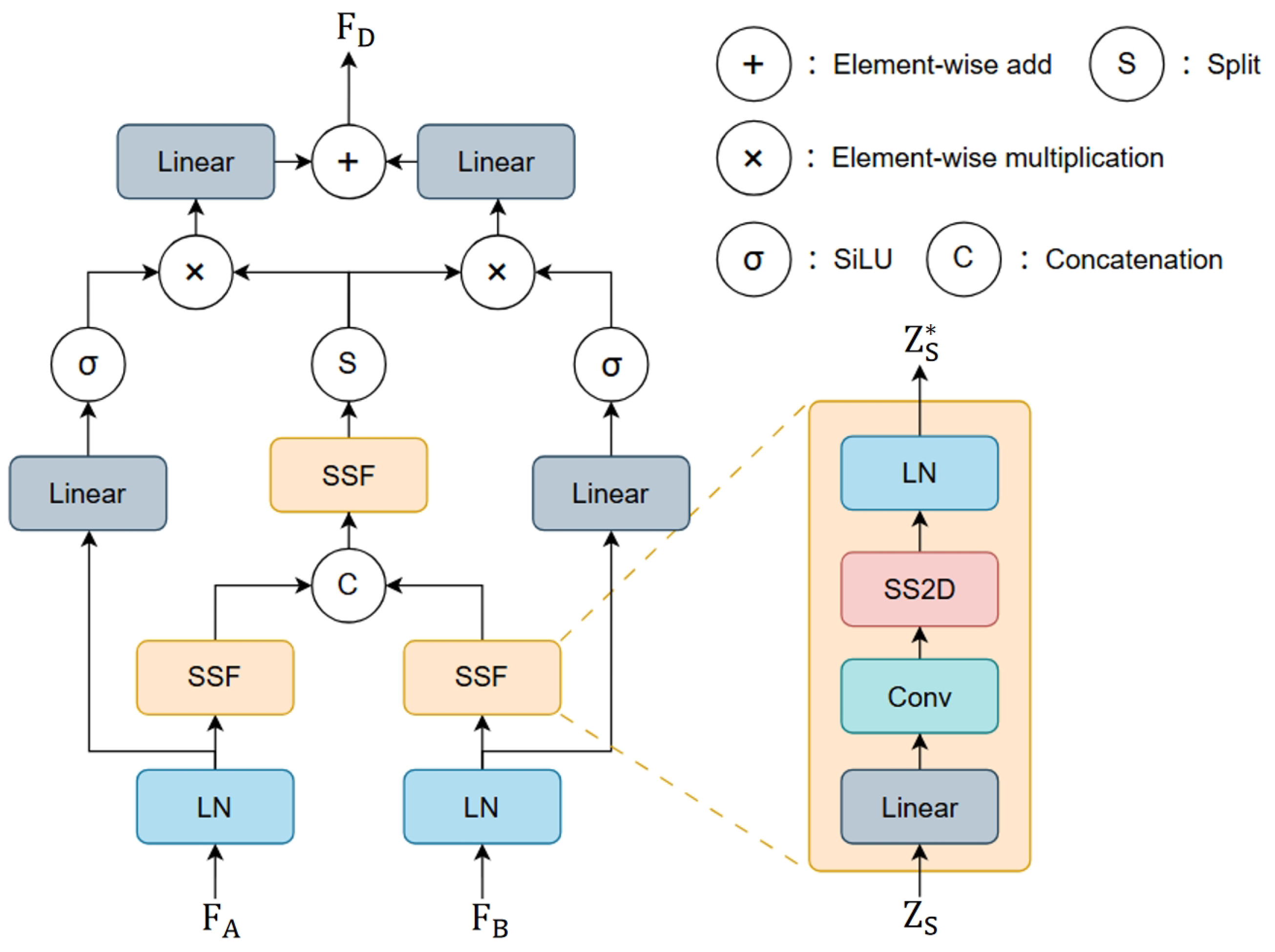
Inspired by Vmamba [42], we propose the State Space Feature (SSF) module, which aims to capture global dependencies through 2D selective state space modeling, thereby obtaining more robust feature representations under complex backgrounds and diverse disturbances. As illustrated in Figure 2, the SSF module consists of four components: First, a linear layer expands the channel dimension of the input features to enhance representational capacity. Second, a convolutional layer combined with a non-linear activation function extracts local contextual information. Subsequently, the SS2D operation is introduced to model long-range spatial dependencies. Finally, layer normalization is applied to enhance feature stability. Formally, given an input feature Z S , the computational process of the SSF module is defined as:
Z S = LN ( SS 2 D ( Conv ( Linear ( Z S ) ) ) )
Building upon this, the DTM module leverages the SSF module to capture the spatio-temporal relationships within bitemporal image features. Given the input bitemporal features F A and F B , they are first normalized using layer normalization to obtain F a and F b . Each is then processed by an individual SSF module to derive its respective global state representations. Subsequently, these two global state representations are concatenated along the channel dimension. Another SSF module is applied to this concatenated feature to model cross-temporal global dependencies and semantic discrepancies, yielding a common feature representation. This common feature is then split evenly along the channel dimension into two sub-features, S A and S B , which correspond to the fusion responses for image A and image B, respectively:
S A , S B = Split ( SSF ( Concat ( SSF ( F a ) , SSF ( F b ) ) ) )
Subsequently, we introduce a feature transformation branch. This branch performs a fully connected computation on the inputs F a and F b , respectively, and incorporates the SiLU activation function to introduce non-linearity, thereby enhancing the model’s expressive capability. Subsequently, the fused response features and the transformed features undergo element-wise multiplication. This mechanism enables the two temporal phases to adaptively emphasize regions relevant to change based on their own semantic characteristics, yielding change features for the two phases. Finally, the results from the two branches are linearly projected and summed pixel by pixel to output the resulting change feature F D .
F D = Linear ( S A SiLU ( Linear ( F a ) ) ) + Linear ( S B SiLU ( Linear ( F b ) ) )
By incorporating the 2D selective scan state space modeling mechanism, the DTM module achieves explicit long-range dependency modeling and global semantic alignment between the bitemporal features. This module sequentially performs state modeling of the bitemporal features, learning of common representations, and reconstruction of differential features during the feature extraction process. Consequently, it captures the semantic correlations of changed regions at a global scale. The output global change features provide a stable and discriminative foundation for subsequent multi-scale refinement modeling and edge interaction fusion.

3.4. Multi-Scale Perception Module

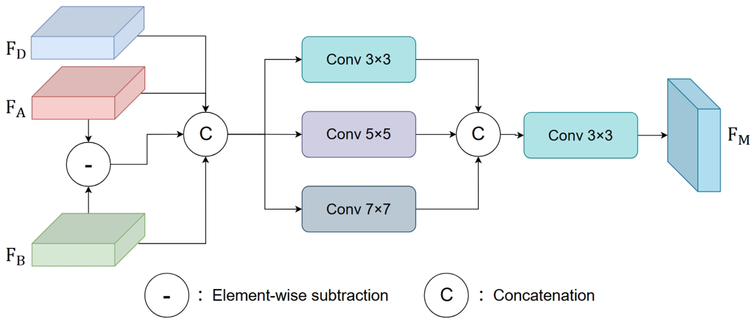
In the change detection task for geological hazards, relying exclusively on global features often proves inadequate for addressing the diverse change patterns inherent in complex scenarios. For example, landslides involve both the overall displacement of the land surface and localized texture perturbations. Similarly, hazardous rock mass changes encompass both weathered regions and minor block movements. To enhance the characterization of fine-grained changes on the basis of the global semantic change features provided by the DTM module, this paper proposes a Multi-Scale Perception (MSP) module. This module refines the modeling of cross-temporal contextual differences through a multi-scale convolutional architecture, effectively augmenting the representational capacity of the change features. This design enables the model to balance global consistency with local sensitivity. A schematic diagram of the MSP module is shown in Figure 3.
Specifically, the MSP module utilizes four features: the global change feature computed by the DTM module, the differential feature of the bi-temporal images, and the bi-temporal image features themselves. First, these four features are concatenated along the channel dimension to form a joint feature representation. Subsequently, the MSP module processes this joint feature through three parallel convolutional branches for multi-scale modeling. The kernel sizes of these branches are 3 × 3 , 5 × 5 , and 7 × 7 , yielding feature maps F 3 , F 5 , and F 7 , respectively. Through this design, the MSP module effectively leverages the global change perception capability of the DTM module while simultaneously enhancing the representation of local structures via multi-scale convolutions. This enables precise extraction of change features even in scenarios characterized by irregular and diverse morphological changes. The outputs of the three branches are then concatenated along the channel dimension and integrated using a 3 × 3 convolution for feature fusion and compression, producing the enhanced change feature F M . This process is formulated as follows:
F M = σ ( BN ( Conv 3 × 3 ( Cat ( F 3 , F 5 , F 7 ) ) ) )
The MSP module further refines the hierarchical expression of cross-temporal feature differences, strengthening the model’s ability to perceive subtle changes and complex shapes. The resulting multi-scale enhanced features provide a richer and more refined feature representation for the subsequent edge–change interaction and frequency-domain fusion.

3.5. Edge-Change Interaction Module

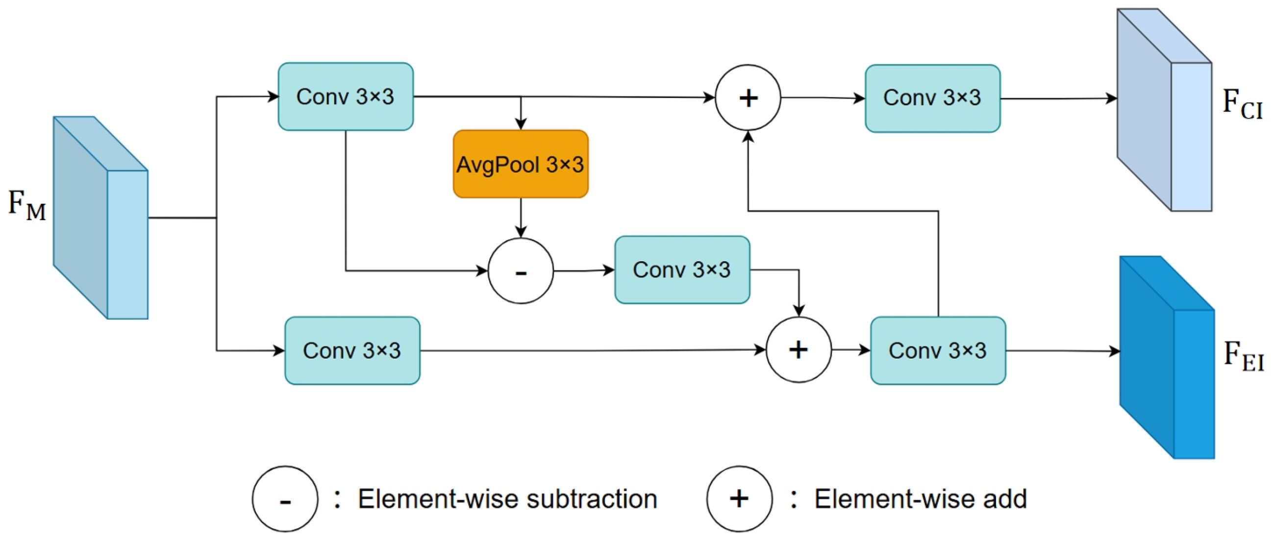
In geological hazard change detection, changed regions are often intertwined with complex backgrounds. Furthermore, some change boundaries are rugged and accompanied by fine-grained edge perturbations, making it difficult to accurately identify them. To address this challenge, we propose an Edge–Change Interaction (ECI) module. This module leverages the complementary relationship between change features and edge features at the feature level. Through a bidirectional interaction mechanism, it achieves mutual enhancement of both edge and change features, thereby improving the model’s capacity to delineate change region boundaries. A schematic diagram of the ECI module is shown in Figure 4.
Specifically, the ECI module first processes the input feature F M through parallel 3 × 3 convolutions to generate the initial features for the change branch and the edge branch, denoted as F ci and F ei , respectively. We aim to enhance the edge branch using edge information derived from the change branch. To this end, a 3 × 3 average pooling is first applied to the initial change feature F ci to obtain a locally smoothed background representation. This representation is then subtracted from the initial change feature, and a convolutional operation is applied to adjust the representation of the resulting difference feature, yielding an edge-difference feature. This operation effectively suppresses low-frequency background information while highlighting regions with significant gradients (i.e., edge regions). Finally, the edge-difference feature is added to the initial edge feature F ei , and the result is adjusted by a 3 × 3 convolution. This guides the edge branch to focus on the genuine boundaries of the changed regions, producing the refined change-edge feature F EI . This process establishes a unidirectional information flow from the change branch to the edge branch, enabling the edge branch to precisely locate change edges with the aid of the edge-difference feature.
F EI = Conv 3 × 3 ( F ei + ( F ci Conv 3 × 3 ( Avg 3 × 3 ( F ci ) ) ) )
Subsequently, the edge feature F EI is passed back to the change branch. It is additively fused with the initial change feature F ci , thereby supplementing fine-grained boundary information at the semantic level. This fused feature is then further refined via a convolution to produce the final enhanced change feature F CI . Through this bidirectional interaction mechanism, the change branch not only perceives the overall semantics of the changed region but also enhances its sensitivity to boundaries via feedback from the edge branch, resulting in more accurate change localization.
F CI = Conv 3 × 3 ( F ci + F EI )
Furthermore, to enhance the discriminative capability of the edge branch, we introduce an edge supervision constraint during the training phase. The output edge feature is aligned with a manually constructed edge label, and an edge loss function is computed. This supervision signal enables the edge branch to learn the spatial boundaries of genuine changes more accurately, thereby providing more reliable edge guidance to the change branch during their interaction.

3.6. Frequency-Domain Change Fusion Module

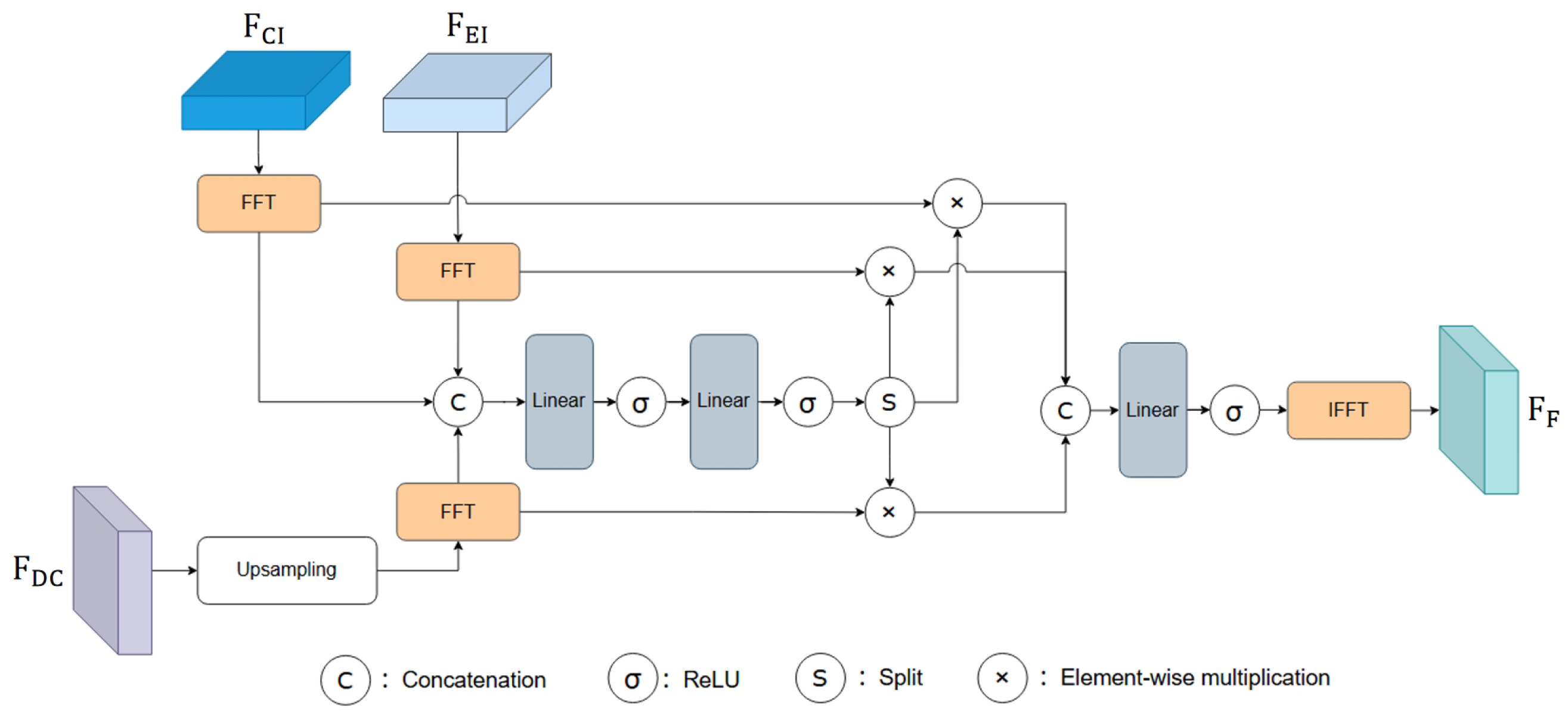
In change detection, deep and shallow features exhibit complementarity. Effectively balancing the contributions of these different features during fusion poses a significant challenge. Edge features can play a crucial role in this process, as they can provide explicit boundary constraints for the fusion of deep and shallow features, thereby mitigating localization deviation and boundary blurring. Simultaneously, the frequency domain possesses the ability to decompose low-frequency and high-frequency components. Leveraging joint frequency-domain modulation during fusion can effectively enhance both global structural information and textural details, consequently improving change detection accuracy. Building upon this rationale, this paper proposes a Frequency-domain Change Fusion (FCF) module. By harnessing the synergistic effect of edge constraints and frequency-domain fusion, the FCF module achieves adaptive decoding of multi-level features. A schematic diagram of the FCF module is shown in Figure 5.
Given the input change feature F CI , edge feature F EI , and the upsampled deep change feature F DC , a 2D Fast Fourier Transform (FFT) is first applied to each of them to obtain their complex representations in the frequency domain, denoted as F CI f , F EI f , and F DC f . Their spectra are then concatenated along the channel dimension to form a joint frequency-domain feature, thereby aggregating semantic change, edge structure, and deep contextual information simultaneously in the frequency space. Inspired by frequency-domain attention modeling approaches like AFNO [51], this study introduces a learnable, per-frequency-component modulation mechanism on the joint spectral feature. Specifically, a Multi-Layer Perceptron (MLP) is used to non-linearly map the joint spectrum, generating corresponding complex modulation weights M C , M E , and M D for each frequency component. This allows the model to adaptively adjust the contribution ratio from the three feature streams for different frequency components, selectively enhancing or suppressing low-frequency semantic information and high-frequency boundary details in the frequency domain, thereby improving the discriminativity and robustness of the feature representation.
M C , M E , M D = Split ( ReLU ( Linear ( ReLU ( Linear ( Concat ( F CI f , F EI f , F DC f ) ) ) ) ) )
After obtaining the frequency-domain modulation weights, they are applied to the corresponding change, deep, and edge spectrum features via element-wise complex multiplication. The weighted spectra are then concatenated along the channel dimension to form the fused spectrum. This fused frequency-domain feature is passed through a fully connected layer to adjust its channel structure, and then transformed back to the spatial domain via the Inverse Fast Fourier Transform (IFFT), yielding the frequency-fused feature F C , as formulated below. This mechanism enables the model to explicitly control the balance between low-frequency and high-frequency information in the spectral dimension, thereby balancing global structural consistency and local boundary sensitivity.
F C = IFFT ( Linear ( Concat ( M C F CI f , M E F EI f , M D F DC f ) ) )
Finally, the recovered frequency-fused feature is added to the three input features, and the result is further refined by a 3 × 3 convolution to produce the final fused output feature. This frequency-domain fusion strategy effectively combines the advantages of both spatial and frequency representations, achieving a superior balance between global semantic understanding and detailed boundary delineation, which significantly enhances the overall performance of change detection.
The Frequency-domain Change Fusion (FCF) module, by introducing a learnable multi-feature modulation mechanism in the frequency space, achieves the adaptive fusion of multi-level change features and edge features. It effectively coordinates the expression of low-frequency structural information and high-frequency boundary details, strengthening local texture and boundary features while preserving global semantic consistency. Consequently, it produces the final change detection result with higher discriminative power and robustness.

4. Experiments

4.1. Datasets

The performance of the proposed MSMCD model is evaluated on three distinct change detection datasets: the public GVLM-CD and WHU-CD benchmarks for landslide and building change analysis, respectively, and a self-constructed TGRM-CD dataset focusing on hazardous rock mass changes. This suite of datasets enables a comprehensive assessment of the model’s capability in handling diverse geological disaster scenarios.

4.1.1. GVLM-CD Dataset

GVLM-CD [52] is the first large-scale public benchmark dataset designed for ultra-high-resolution landslide mapping, specifically crafted to capture surface changes before and after landslide disasters. This dataset covers several typical regions that experienced severe natural disasters between 2010 and 2021, including Aloy, Asakura, and Ashaga. It comprises 17 pairs of bi-temporal Very High-Resolution (VHR) RGB images with a resolution of 0.59 m, sourced from the Google Earth service. During the data preprocessing stage, these large-format images were cropped into non-overlapping image patches of size 256 × 256 pixels. We split all data into 4558/1519/1519 pairs of images for training, validation, and testing, respectively. The dataset reflects the surface differences before and after landslide events across different regions and time periods, featuring a rich variety of landform types and disaster scenarios.

4.1.2. WHU-CD Dataset

The WHU-CD dataset primarily focuses on building reconstruction changes in the same area over several years following an earthquake, effectively enabling the assessment of urban recovery and reconstruction progress after a seismic disaster. This dataset consists of a pair of large-format aerial images with dimensions of (32,507 × 15,354) pixels and a spatial resolution of 0.2 m per pixel. For experimentation, these images are divided into non-overlapping patches of 256 × 256 pixels. We split all data into 5947/743/744 pairs of images for training, validation, and testing, respectively. The dataset covers a typical area in New Zealand affected by a magnitude 6.3 earthquake in February 2011. Researchers acquired bi-temporal aerial images with a spatial resolution of 0.2 m in 2012 and 2016, and performed meticulous manual annotation to identify building changes caused by seismic damage and subsequent reconstruction.

4.1.3. TGRM-CD Dataset

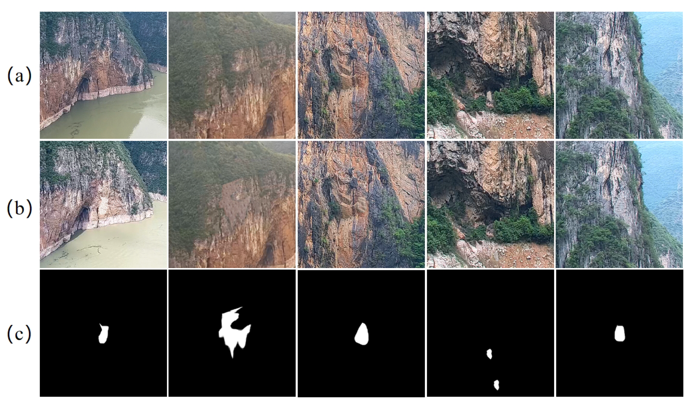
The TGRM-CD (Three Gorges Rock Mass Change Detection) dataset constructed in this paper was collected by the Chongqing Institute of Geology and Mineral Resources using Unmanned Aerial Vehicles (UAVs), covering multiple typical hazardous rock mass areas within the Three Gorges Reservoir area, as shown in Figure 6. During the data acquisition process, we obtained multi-temporal high-resolution images under different periods and diverse lighting conditions and weather environments to fully reflect the complexity and diversity of image data in real geological hazard monitoring scenarios.
The selection of hazardous rock mass areas primarily focused on typical sections that pose potential threats to navigation safety and exhibit high geological hazard risks. These areas feature large terrain relief and complex rock mass structures, making them highly prone to hazardous changes such as collapses and spalling, thus possessing strong research representativeness and practical application value. During the annotation process, following the professional guidance of experts in the field of geology and based on the actual evolutionary characteristics of hazardous rock masses, we strictly distinguished genuine changes from pseudo-changes. By comprehensively comparing images from different periods with field survey results, we retained only the change information related to the genuine physical evolution processes of the rock masses, ensuring the accuracy and scientificity of the annotation results. The final annotated change types mainly include rock mass surface changes caused by long-term weathering and spalling, and changes resulting from block displacement or collapse. These two types of changes are directly linked to potential geological hazard risks, providing reliable data support for subsequent navigation safety assessments and geological hazard early warning.
Considering the diverse morphology of hazardous rock masses and the variations in illumination conditions in real-world environments, we introduced a dual enhancement strategy involving both geometric and optical transformations during the data construction process. This strategy aims to increase the diversity of the dataset and improve the robustness of model training. The geometric augmentation component includes elastic deformation and grid distortion, which simulate local morphological differences and imaging distortions of rock masses. The optical augmentation component involves optical distortion, gamma correction, and brightness adjustment, designed to reproduce imaging variations under different weather and lighting conditions. This enhancement strategy effectively expands the sample space while preserving the authenticity of geological change characteristics, thus improving the model’s generalization capability in complex scenarios. The TGRM-CD dataset comprises 15,184 pairs of image samples, each with a resolution of 256 × 256 pixels. We divided the data into training, validation, and testing sets, with 9110, 3037, and 3037 pairs of images, respectively. This dataset covers various hazardous rock mass change scenarios and includes their corresponding precise annotation results.

4.2. Experiment Setting and Evaluation Metrics

The proposed model was implemented using the PyTorch (v2.1.0) framework and trained on an NVIDIA RTX 3090 GPU. We employed the Adam optimizer for training, with a batch size of 6 over 100 epochs. The best-performing model checkpoint, selected based on the highest F1-score on the validation set, was used for testing.
The model training encompasses two tasks—change map prediction and edge map prediction—that utilize two types of supervisory signals: change labels and change edge labels, respectively. The edge labels are generated by performing morphological erosion operations on the binary change masks. Specifically, we first erode the binary mask using a 3 × 3 structural element. The edge supervision label is then obtained by calculating the difference between the masks before and after erosion, extracting a closed boundary map located within the change regions. This method ensures spatial consistency between the edge labels and the semantic change areas, while also avoiding the need for additional manual annotation. The loss function for both tasks is a weighted sum of cross-entropy loss and dice loss, defined as follows:
L total = λ 1 L ce + λ 2 L dice
L ce = 1 N i = 1 N y i log ( y ^ i )
L dice = 1 2 i = 1 N y i y ^ i i = 1 N y i + i = 1 N y ^ i
where λ 1 and λ 2 denote the weighting coefficients of the loss function, y i is the ground truth label for the i-th pixel, y ^ i represents the predicted probability for the i-th pixel, and N indicates the total number of pixels. According to the ablation study on loss function coefficients in Section 4.4.2, we set λ 1 and λ 2 to 0.5.
In the experiments, we adopted four key evaluation metrics: precision (Pre), recall (Rec), F1-score, and Intersection over Union (IoU). Precision reflects the proportion of true positive pixels among all pixels predicted as positive. Recall indicates the proportion of true positive pixels among all actual positive pixels in the ground truth. The F1-score is the harmonic mean of precision and recall, providing a comprehensive assessment of the model’s precision and recall capabilities. IoU measures the degree of overlap between the predicted positive region and the true positive region. These metrics can be formally defined as follows:
Pre = TP TP + FP
Rec = TP TP + FN
F 1 = 2 × Pre × Rec Pre + Rec
IoU = TP TP + FP + FN
In this paper, TP, TN, FP, and FN denote true positive, true negative, false positive, and false negative pixels in the prediction result, respectively.

4.3. Comparison and Analysis

To validate the effectiveness in change detection tasks, this section selects a variety of methods for comparison, including CNN-based methods (FC-EF series [27], IFNet [28], SNUNet [53], ISDANet [54]), Transformer-based methods (BIT [34], ChangeFormer [55], MSCANet [38], Paformer [20], ACABFNet [56]), and Mamba-based methods (RS-Mamba [43], ChangeMamba [44], CDMamba [57], MF-VMamba [58]).

4.3.1. Quantitative Results

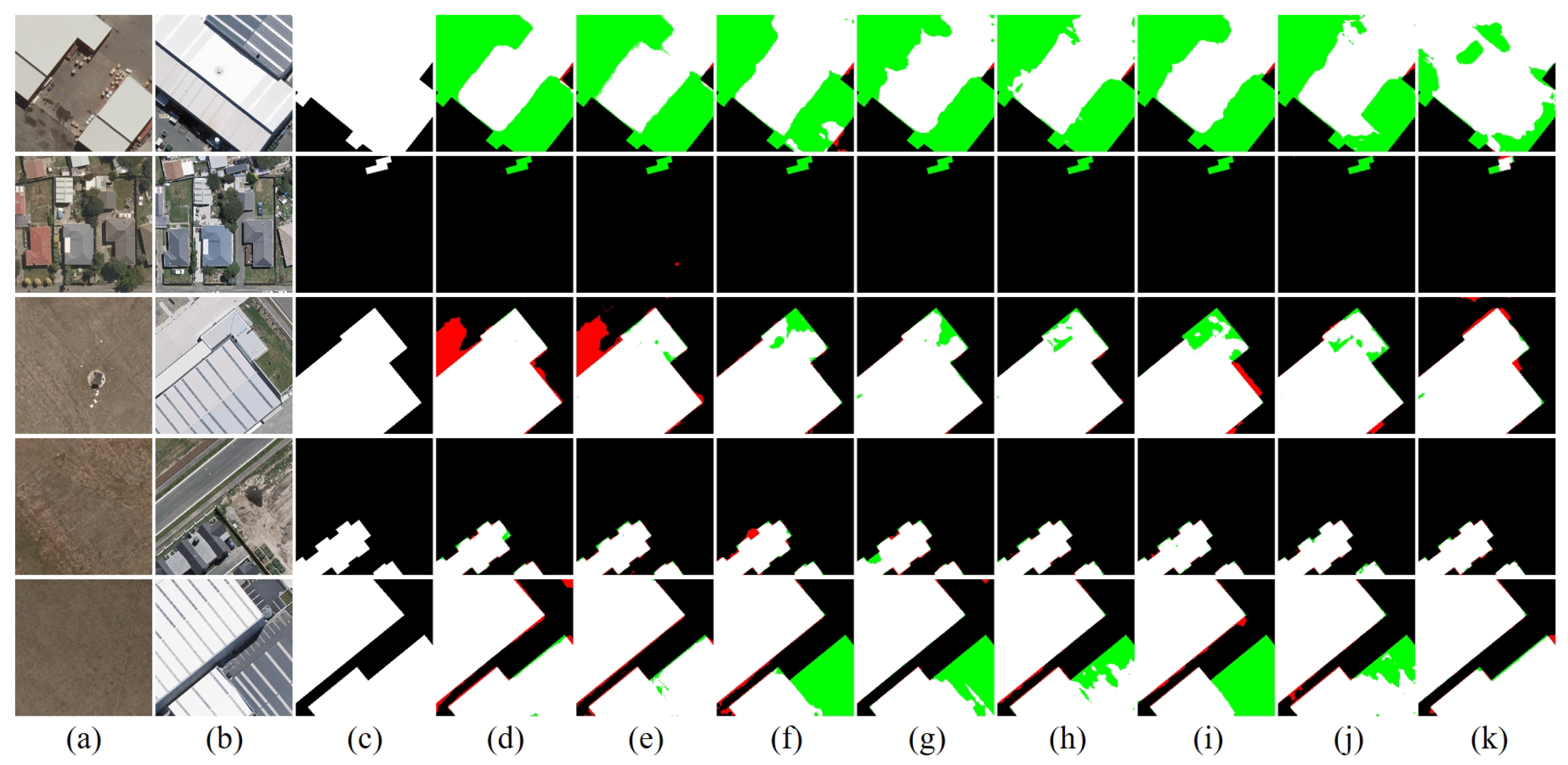
Table 1 and Table 2 report the quantitative comparison of IoU, F1-score, recall, and precision for different methods on the three datasets. We consider the F1-score and IoU as the primary evaluation metrics. The best results are highlighted in bold. A comprehensive analysis of the experimental results across the three datasets demonstrates that our proposed MSMCD achieves the best performance on the vast majority of evaluation metrics. Notably, on the overall performance metrics—IoU and F1-score—our method significantly outperforms all competing methods across all three datasets, validating its effectiveness and practical utility in practical application scenarios such as geological hazard assessment and urban reconstruction monitoring.
On the GVLM-CD dataset, our method achieved the best performance in the table for both IoU (80.23%) and F1-score (89.03%), surpassing the second-best method, RS-Mamba, by 1.01% and 0.62%, respectively. The simultaneous lead in these two overall metrics indicates that under the conditions of noisy backgrounds and topographic relief in this dataset, our model achieves substantial improvements in both accurate detection and regional coverage dimensions. In terms of individual metrics, precision (89.02%) and recall (89.03%) are essentially balanced. Specifically, recall is 0.10% higher than the second-best method, FC-Siam-Conc (88.93%), achieving a slightly higher detection rate without significantly sacrificing precision. It should be noted that precision is 1.13% lower than CDMamba (90.15%). However, given the simultaneous improvement in F1/IoU, the overall result demonstrates a superior precision–recall trade-off. Compared with methods that tend to optimize a single metric, our approach achieves higher comprehensive effectiveness on GVLM-CD through a more balanced P/R combination, which is crucial for suppressing pseudo-changes while maintaining a high recall rate.
On the WHU-CD dataset, the proposed method achieved optimal performance in overall evaluation metrics, with IoU and F1 scores reaching 85.50% and 92.18%, respectively, representing improvements of 1.39 and 0.83 percentage points compared to the suboptimal method, CDMamba. In other metrics, the recall was 90.01%, which is 1.19 percentage points lower than the optimal method ISDANet, while the precision was 94.47%, only 0.05 percentage points lower than the optimal method ChangeMamba. Although the proposed method did not achieve optimal results simultaneously in both recall and precision, it demonstrated a favorable balance between the two, showing significant advantages in overall detection performance. This indicates that the proposed method not only exhibits strong adaptability to natural scenarios, such as mountainous terrain, but also demonstrates a robust capability in handling complex urban features.
On our self-constructed TGRM-CD dataset, our method achieved the highest IoU (77.33%) and F1-score (87.22%), outperforming the suboptimal method, CDMamba, by 1.68% and 1.23%, respectively. This significant performance improvement is attributed to the model’s powerful representational capacity for the complex topographic features of hazardous rock masses. A recall of 88.09%, which is 0.81% higher than the second-best method, FC-Siam-Diff (87.28%), demonstrates a comprehensive capture of genuine changes in hazardous rock masses, can detect subtle variations caused by weathering and spalling. Meanwhile, precision remained at a high level of 86.36%, only 0.33% lower than the top value (ACABFNet), indicating that while enhancing detection sensitivity, the model effectively suppresses pseudo-changes caused by terrain relief and shadow variations. These results demonstrate that in geological hazard scenarios characterized by complex landforms and weak target features, the multi-stage detection mechanism adopted by MSMCD can effectively distinguish real changes from background interference, significantly improving the detection coverage of change areas while controlling the false positive rate, thus providing reliable technical support for the early identification of geological hazards.
The experimental results above confirm the superior detection accuracy and robustness of MSMCD. To further evaluate its practicality in real-world deployments, we analyzed the computational and memory efficiency of the model using the number of floating-point operations (FLOPs) and the number of parameters. FLOPs are calculated with a pair of input images sized 1 × 3 × 256 × 256. As shown in Table 2, MSMCD has 6.1 M parameters and 9.7 G FLOPs. Compared with other models, these metrics are relatively low, indicating that the model has favorable lightweight properties. Although multiple functional modules (DTM, MSP, ECI, FCF) are introduced, the overall complexity is still effectively controlled, mainly for the following reasons: First, the model adopts a hierarchical processing architecture, with each module appearing only once in each layer, responsible for different functions such as global dependency modeling, local difference enhancement, edge constraint, and frequency-domain fusion, avoiding redundant stacking of modules; Second, the feature extraction stage uses the lightweight backbone network MobileNetV2, and the number of channels in the feature maps of each layer is simplified to 12, 16, 24, and 32, effectively controlling the scale of parameters. Therefore, MSMCD maintains accurate change detection capabilities while having low computational complexity, which can better meet the needs of practical applications.

4.3.2. Qualitative Results

In the qualitative analysis section, we compare the visual results of different methods on the GVLM-CD, WHU-CD, and TGRM-CD datasets to intuitively demonstrate their performance differences in complex scenarios.
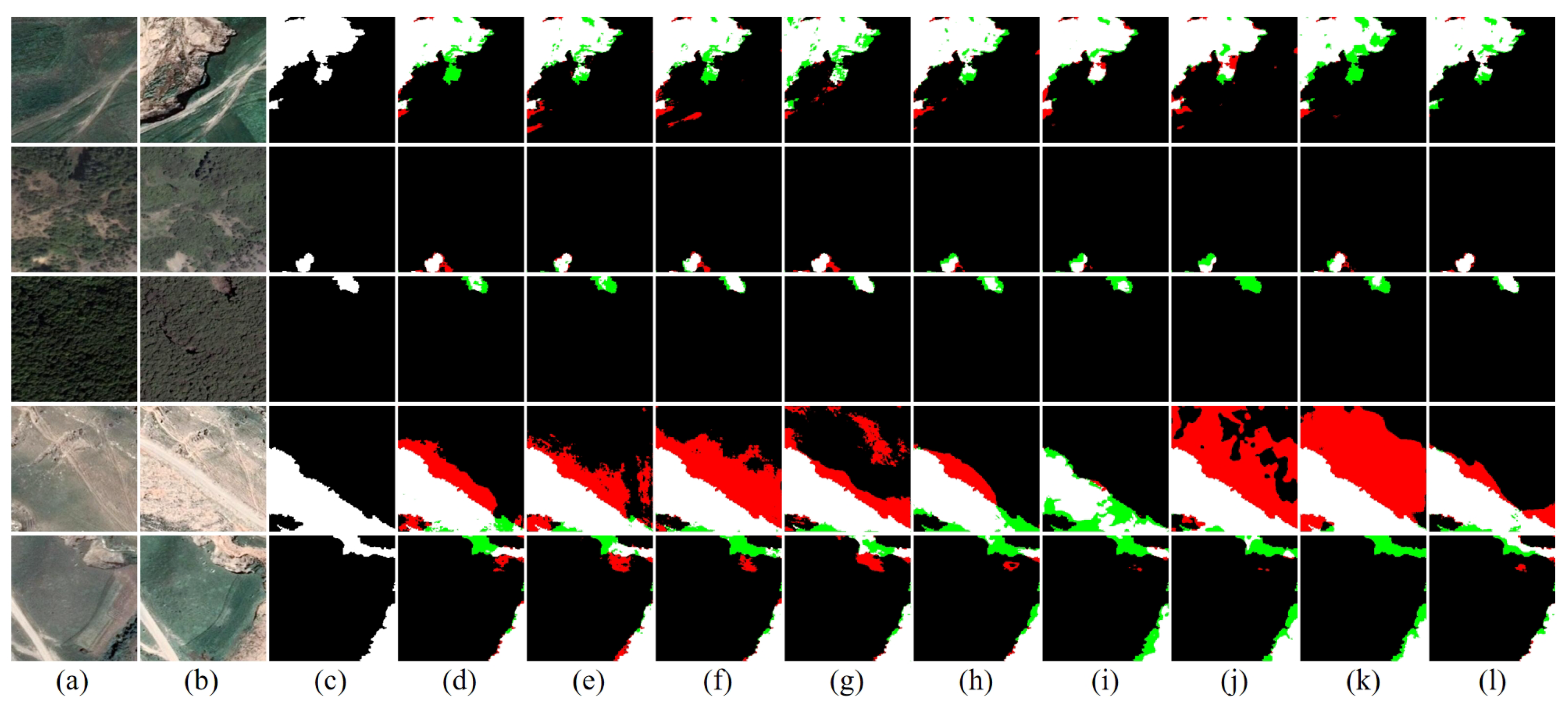
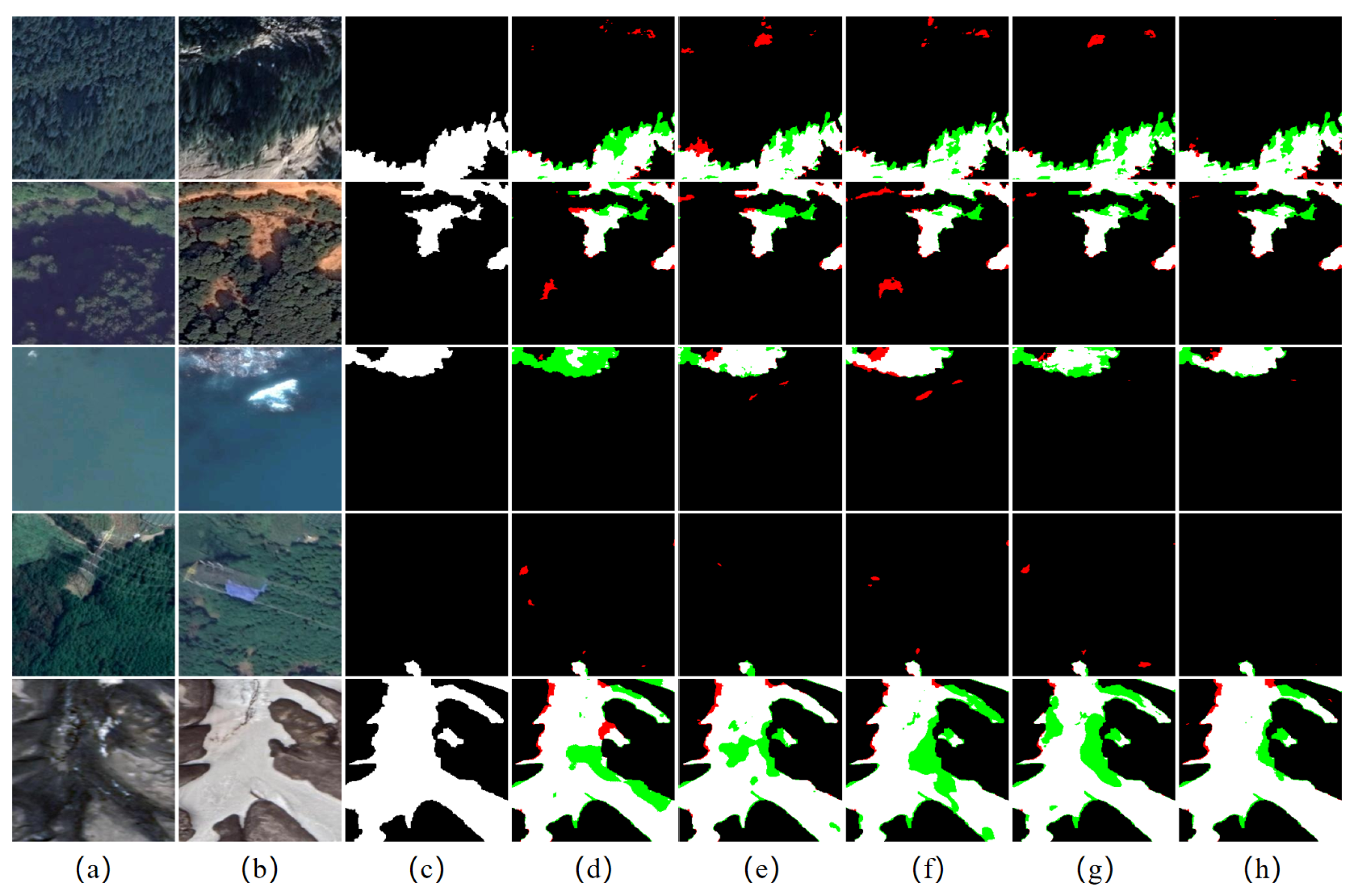
In Figure 7 and Figure 8, the change boundaries shown in rows 1 and 5 are rugged and indistinctly interwoven with the background, containing some interference similar to the change. Although many methods can detect the change regions, they also suffer from both false positives and false negatives. In contrast, our method extracts the change regions more accurately. The change regions in rows 2 and 3 are relatively small and accompanied by brightness differences between the two temporal images. Many models showed false negatives, and some even failed to detect the change at all. However, our method accurately identified these change regions, demonstrating its strong performance even for small-scale targets. The change regions in row 4 are highly similar to the background, leading to a large number of false positives in many models. Our model most accurately located the landslide area. Overall, our method demonstrates superior visual performance on the GVLM-CD dataset, effectively reducing false positives and false negatives. The detection maps generated by our model closely match the actual landslide distribution.
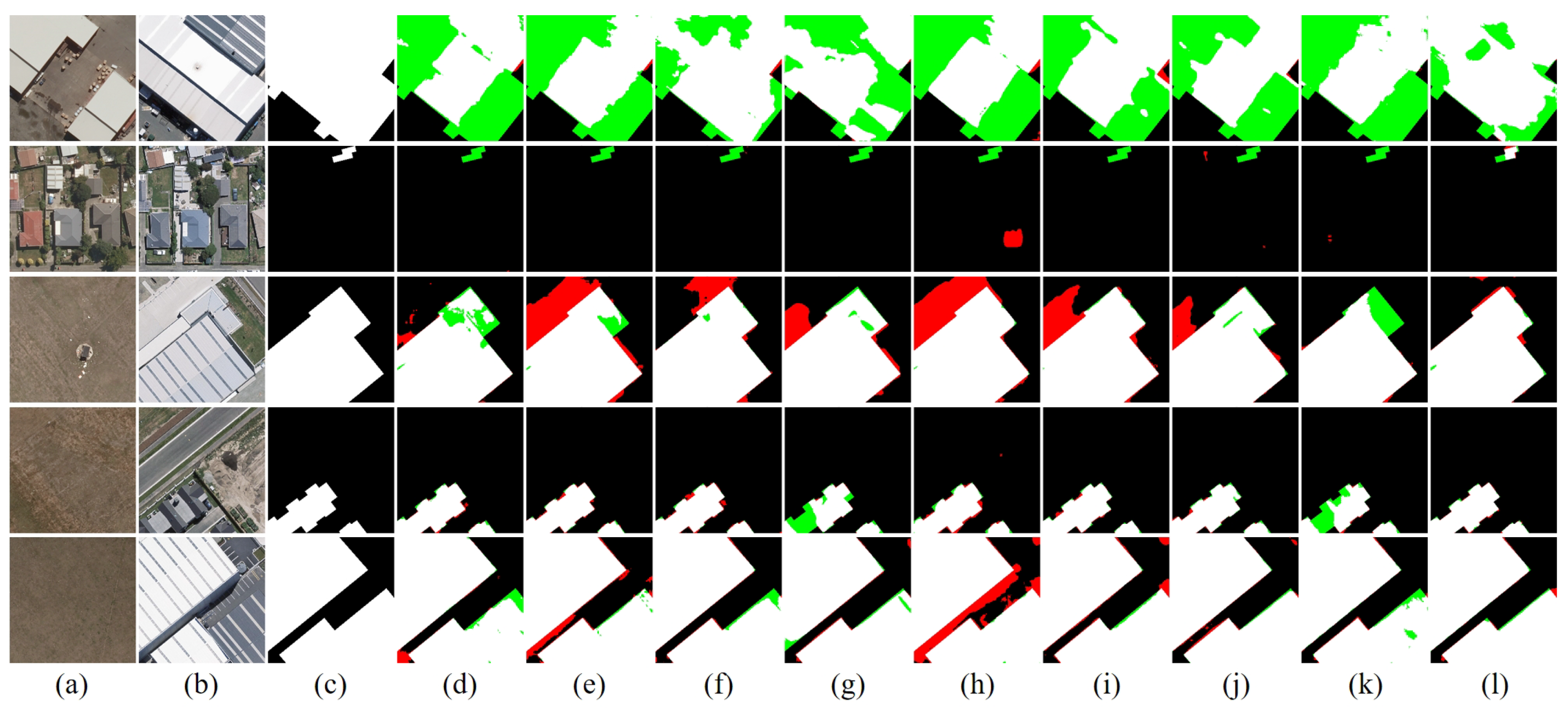
In Figure 9 and Figure 10, for the image in row 1, the buildings before and after the change exhibit similarity, which results in numerous missed detections in most methods. Our method achieves the fewest omissions, demonstrating discriminative ability under such change similarity conditions. The change regions in row 2 are small and set against a background dense with buildings. Some methods exhibit both missed and false detections, whereas our method successfully captures these subtle changes while avoiding false alarms. In the images shown in rows 3 and 5, although the pre-change image background is simple, the high similarity between buildings and non-building features (e.g., roads) in the post-change image, combined with the large change area, causes numerous methods to produce extensive false positives and false negatives. For the image in row 4, the building features in the post-change image are more distinct than in rows 3 and 5, but the change area is smaller and has more complex boundary corners. Our method again achieves the most precise detection. These results confirm that our method delivers the best performance for building changes in the WHU-CD dataset.
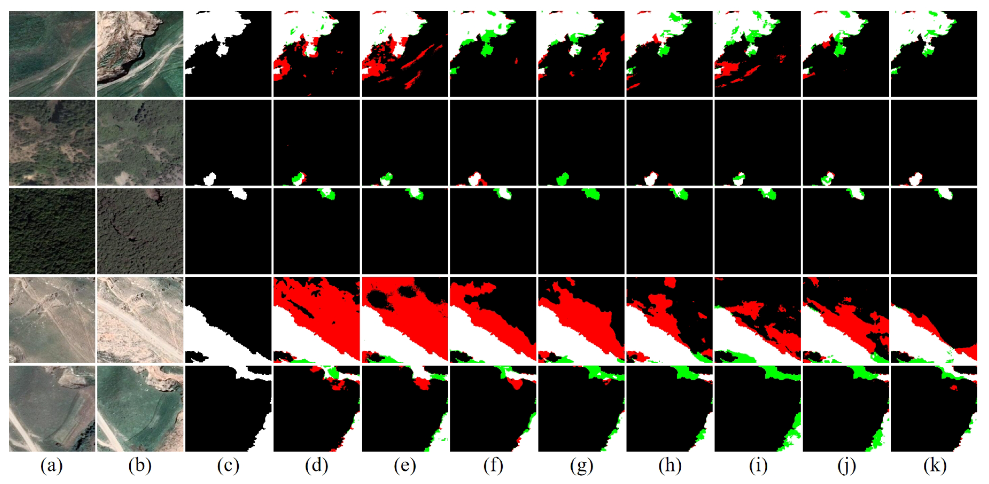
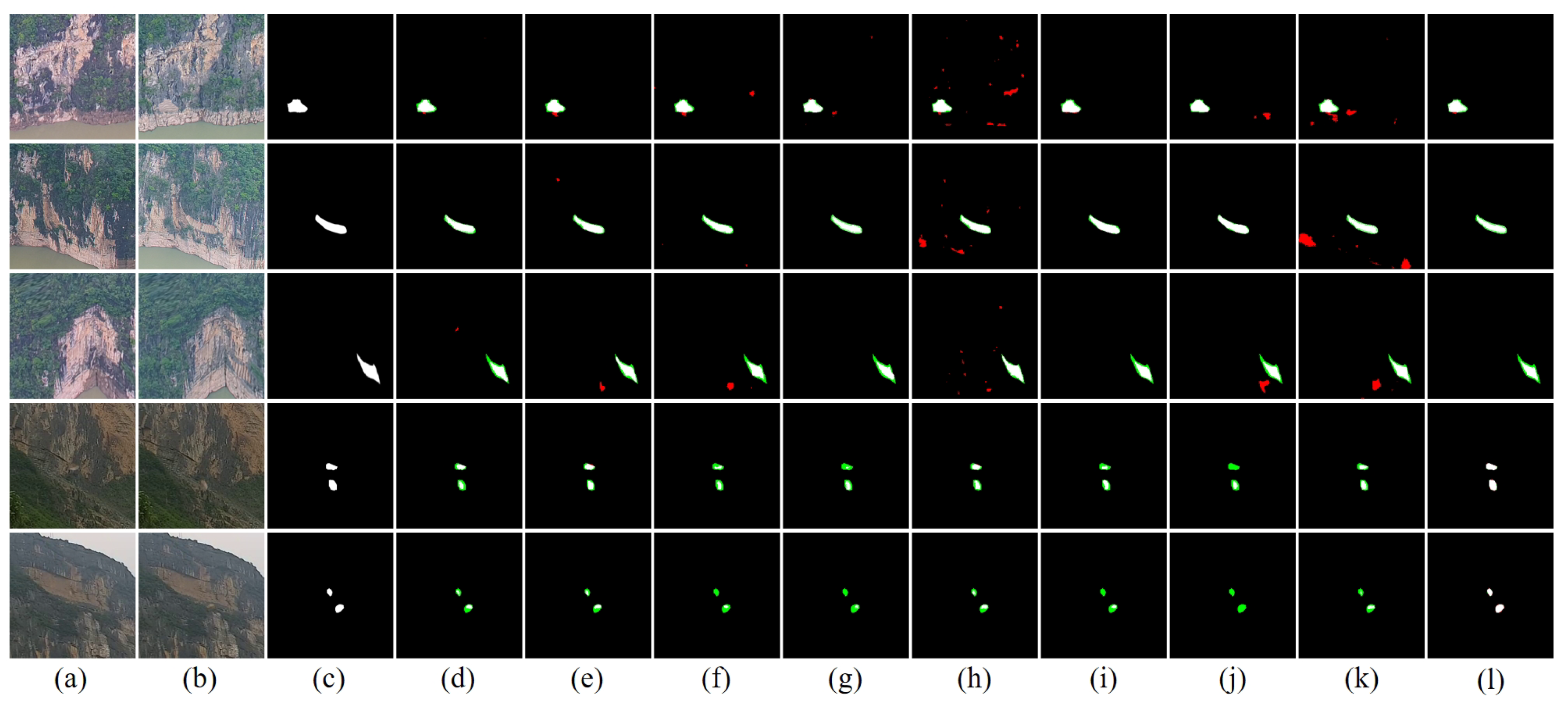
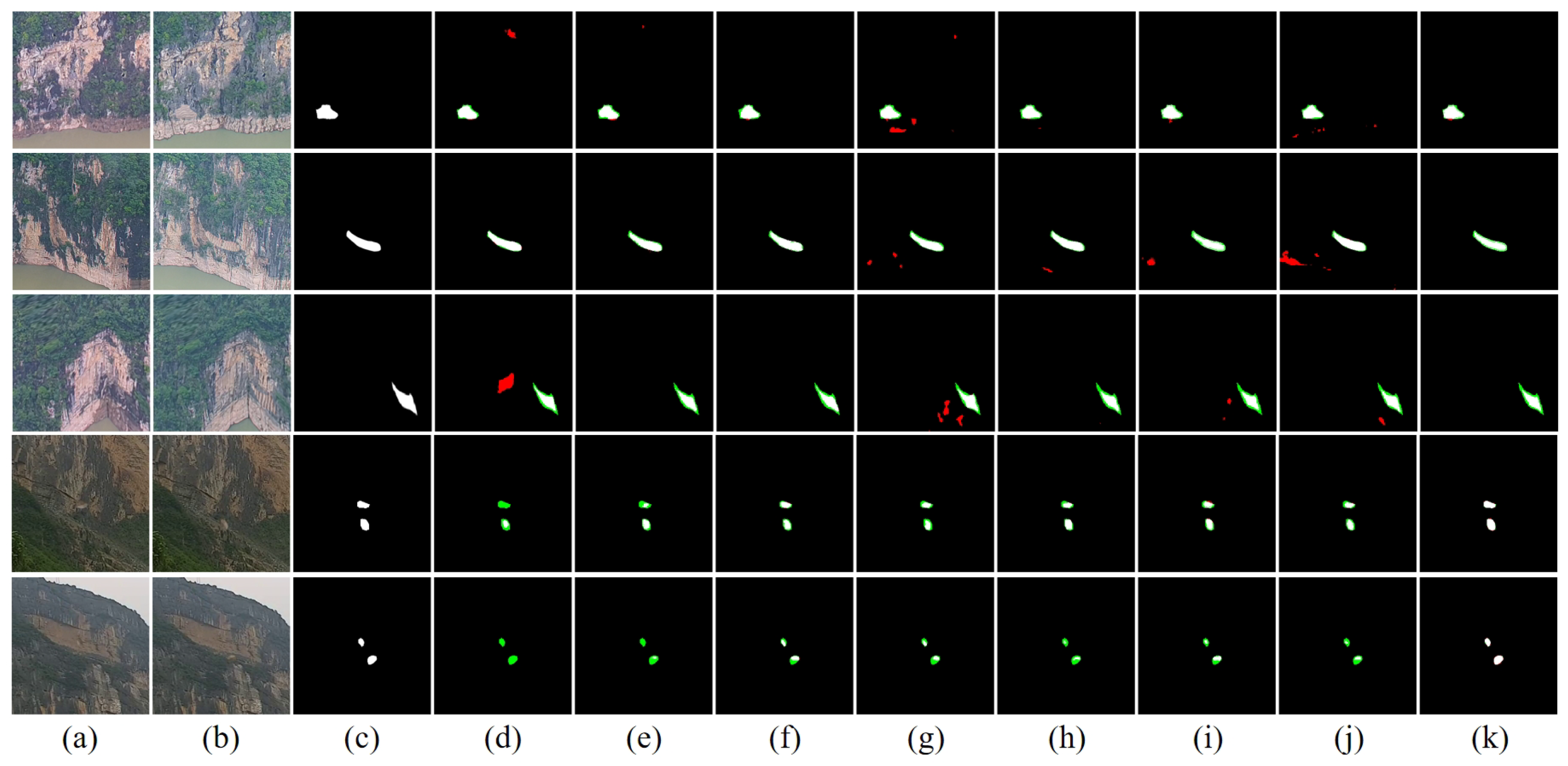
In Figure 11 and Figure 12, the images in rows 1, 2, and 3 are affected by certain illumination variations and complex mountain textures, leading to varying degrees of false detections in most methods. Our method effectively separates illumination differences from genuine geological changes, accurately extracting the change regions. In the images shown in rows 4 and 5, the imaging environment is relatively consistent between the temporal phases. The occurring block displacement changes are highly similar to the surrounding background, and the change areas are small, resulting in missed detections by many methods. Our method, while maintaining the integrity and continuity of the changes, successfully identifies these subtle block displacements. Overall, our method achieves a better balance between robustness to complex backgrounds and sensitivity to real changes on the TGRM-CD dataset.
Qualitative results from the GVLM-CD, WHU-CD, and TGRM-CD datasets not only demonstrate the superior performance of the MSMCD model but also provide intuitive visual evidence of its effectiveness in addressing the challenges described in the introduction. First, regarding the challenges of complex backgrounds and imaging interference, the model exhibits robustness. As shown in the visualizations of GVLM-CD (rows 1 and 3) and TGRM-CD (rows 1, 2, and 3), MSMCD effectively suppresses noise caused by illumination variations and complex terrain textures, thus accurately identifying genuine areas of change. Second, addressing the challenges of diverse change types and significant scale differences, the model demonstrates strong detection capabilities across different scales. It performs well on large-scale landslides in GVLM-CD (rows 1 and 4), building changes at different scales in WHU-CD (rows 2 and 5), and small rock mass changes in TGRM-CD (rows 1 and 5). Finally, despite the challenges of blurred boundaries and irregular shapes, the model can generate accurate detection maps even in scenarios where changes are highly similar to the background (as shown in rows 4 and 5 of GVLM-CD and TGRM-CD). These visualizations demonstrate that MSMCD can reliably handle the typical challenges in detecting changes in geological hazards.

4.4. Ablation Studies

4.4.1. Ablation Study on Model Components

To systematically evaluate the specific contribution of each core module in the MSMCD model to the overall performance, we conducted ablation studies on the GVLM-CD dataset. The experiments adopted the same training configuration and data split as the main experiments. By removing the DTM (w/o DTM), MSP (w/o MSP), ECI (w/o ECI), and FCF (w/o FCF) modules, four comparative model variants were constructed, with the full model containing all modules (Full (Ours)) serving as the performance baseline. The quantitative results are detailed in Table 3. The best results are highlighted in bold. The corresponding qualitative visual comparisons are presented in Figure 13.
Effectiveness of the DTM module. In the variant without the DTM module (w/o DTM), the input to the MSP module no longer includes the feature branch from DTM. The experimental results show a significant performance drop in this variant, with IoU and F1-score decreasing by 0.99% and 0.61%, respectively. Concurrently, the recall metric decreased by 2.30%, while precision increased by 1.13%. This indicates that the DTM module, through its powerful capability for modeling global cross-temporal dependencies, is crucial for capturing faint and fragmented real change areas. In its absence, although the model becomes more conservative and reduces some false positives, this comes at the cost of a significant increase in missed detections, leading to a decline in overall performance (IoU/F1). As can be intuitively observed in Figure 10, after removing DTM, the number of false negative regions in the prediction results increases markedly, while some false positives appear in complex background areas, confirming the module’s key role in enhancing the model’s generalizability and robustness.
Effectiveness of the MSP module. We removed the MSP module, which is responsible for local detail enhancement, and fed the output features of the DTM module directly into the ECI module. Compared to the full model, this variant’s IoU and F1-score decreased by 0.74% and 0.46%, respectively, while precision and recall also dropped by 0.21% and 0.71%. This result highlights the importance of the MSP module’s multi-scale convolutional structure for fine-grained contextual comparison, which enhances both the model’s discriminative power and semantic alignment capability, effectively balancing pseudo-change suppression and real change detection in complex backgrounds. As shown in Figure 10, the removal of the MSP module led to increased false negatives and false positives in diverse scenes with an overall decline in detection quality, showing this module’s contribution to enhancing local discriminative ability.
Effectiveness of the ECI module. To validate the role of the edge constraint mechanism, we removed the ECI module, meaning that the model no longer outputs edge features for auxiliary supervision, and the FCF module also lost its edge feature branch. The results show that this variant’s IoU and F1-score decreased by 0.29% and 0.18%, respectively. Notably, its recall increased by 0.37%, slightly higher than the full model, but precision decreased significantly by 0.72%. This suggests that the ECI module, through bidirectional interaction between edges and changes, constrains the outward expansion of predicted boundaries and sharpens change contours, thereby improving localization accuracy and boundary definition. Although it slightly sacrifices some recall rate, it ultimately yields a net gain in IoU/F1 metrics. Figure 10 shows that without ECI, the prediction results exhibit more false positives at the edges of change regions and in the background, confirming the module’s value in improving boundary geometric consistency.
Effectiveness of the FCF module. Finally, we evaluated the role of the frequency-domain fusion strategy by removing the frequency-domain transformation and modulation parts of the FCF module, retaining only simple feature addition and convolution operations. Its performance decreased noticeably, with IoU and F1-score dropping by 0.58% and 0.36%, respectively, and both precision and recall declining synchronously. This result indicates that without frequency-domain processing capability, the model struggles to adaptively balance low-frequency structural information and high-frequency detail components, leading to a weakened ability to suppress background noise while preserving edge details, resulting in suboptimal fusion performance. As shown in Figure 10, without FCF, the model produces more false negatives inside change regions and more false positives in the background, with increased noise and reduced completeness in the predictions.
The ablation studies demonstrate that all four core modules of MSMCD provide substantial and complementary contributions to the final performance. The DTM module establishes the foundation for global cross-temporal representation, significantly improving recall. The MSP module enhances local detail discrimination, achieving a balance between precision and recall. The ECI module optimizes boundary quality and prediction accuracy through edge constraints. The FCF module achieves adaptive fusion of deep semantic and shallow detail features in the frequency domain. The full model achieves optimal performance across all comprehensive quantitative metrics and qualitative results, fully validating the necessity and effectiveness of the proposed multi-stage, multi-dimensional collaborative design.

4.4.2. Ablation Study on Loss Function Coefficients

To validate the impact of different loss function coefficients on model performance, we conducted corresponding experiments on the GVLM-CD dataset. The experimental results are shown in Table 4, where λ 1 represents the coefficient of cross-entropy loss and λ 2 indicates the coefficient of dice loss. The best results are highlighted in bold. The experimental results show that the model achieves the best performance when λ 1 and λ 2 are relatively balanced. Therefore, we choose λ 1 = λ 2 = 0.5 as the final loss function coefficients.

5. Discussion

The MSMCD model proposed in this paper has demonstrated excellent performance across multiple geological hazard change detection tasks, such as landslides, post-earthquake building reconstruction, and unstable rock mass monitoring. This fully validates its powerful change perception capability in complex geological scenarios. However, considering the practical application requirements and technological development trends in geological hazard monitoring, there remains room for further optimization in the model architecture’s interaction mechanisms and its generalization ability across different scenarios. This section will discuss these aspects, aiming to explore directions for future research and improvement.
Firstly, the design of MSMCD integrates multi-dimensional feature processing strategies, including global dependency modeling, local difference enhancement, edge constraints, and frequency-domain fusion. Ablation experiments have confirmed the effectiveness of each module. This synergistic design enables precise detection while maintaining a low parameter count. However, the feature interaction between modules in the current model primarily relies on static operations such as channel concatenation and element-wise addition, lacking a dynamic adaptation mechanism based on feature semantic levels and spatial correlations. This limitation, to some extent, restricts the model’s depth of understanding of complex change patterns. Future research could explore the introduction of dynamic feature interaction strategies to achieve adaptive feature calibration and fusion, thereby more fully unleashing the synergistic potential of multi-dimensional features and further enhancing the model’s discriminative ability.
Secondly, the outstanding performance of MSMCD on existing datasets largely relies on sufficient annotated samples. However, in practical geological hazard monitoring, a significant number of scenarios fall into the categories of few-shot or even zero-shot learning, such as rare hazard types like small-scale rockfalls and gradual land subsidence, as well as unstable rock mass changes in remote areas and compound geological hazards triggered by extreme weather. The feature learning mechanism of the current model is primarily based on statistical patterns from existing samples, making its generalization capability for such sample-scarce or out-of-distribution scenarios challenging. To address this issue, future work could consider integrating the general visual prior knowledge from large models or introducing few-shot learning paradigms such as meta-learning and prompt learning. This would enhance the model’s ability to adapt quickly under limited sample conditions, reduce dependency on large-scale annotated data, and achieve effective recognition of rare change types.

6. Conclusions

This paper addresses the challenges in change detection for geological disaster scenarios, such as complex surface backgrounds and irregular boundary morphology, by proposing a Multi-stage Mamba Change Detection network (MSMCD). The model is centered on the core ideas of global modeling, detail enhancement, edge constraints, and frequency-domain fusion. Through the sequential operation of the DTM, MSP, ECI, and FCF modules, it progressively optimizes the balance between the overall structure and local details in feature representation. Comparative experimental results on typical geological disaster datasets, including landslides, post-earthquake building reconstruction, and unstable rock mass monitoring, demonstrate that MSMCD outperforms existing state-of-the-art methods in metrics such as IoU and F1-score, showcasing excellent change detection performance. Simultaneously, ablation studies validate the rationality of the design of each module and its synergistic effects. However, this study still has some limitations: the dynamic interactivity between different module operations is insufficient, and the multi-stage synergy needs improvement. Additionally, the current detection performance relies heavily on large-scale training data, making it difficult to meet the demands of practical applications. In the future, we will further explore multi-stage dynamic collaborative design and enhance the generalization detection capability for rare geological disaster scenarios, thereby improving engineering application value.

Author Contributions

Conceptualization, L.Q.; methodology, L.Q.; data curation, L.Q., L.W. and L.C.; writing—original draft, L.Q.; writing—review and editing, Q.Z., G.L., W.Y. and H.Z. All authors have read and agreed to the published version of the manuscript.

Funding

This work is supported by the horizontal research project “AI-Based Video Monitoring for Rock Surface Change Detection and Deformation Analysis” in collaboration with the Chongqing Institute of Geology and Mineral Resources, under project number M2024066.

Data Availability Statement

The data presented in this study are available upon request from the corresponding author. The data are not publicly available due to privacy restrictions.

Conflicts of Interest

The authors declare no conflicts of interest.

References

  1. Lv, Z.; Zhang, M.; Sun, W.; Benediktsson, J.A.; Lei, T.; Falco, N. Spatial-contextual information utilization framework for land cover change detection with hyperspectral remote sensed images. IEEE Trans. Geosci. Remote Sens. 2023, 61, 4411911. [Google Scholar] [CrossRef]
  2. Stilla, U.; Xu, Y. Change detection of urban objects using 3D point clouds: A review. ISPRS J. Photogramm. Remote Sens. 2023, 197, 228–255. [Google Scholar] [CrossRef]
  3. Zhu, Q.; Guo, X.; Li, Z.; Li, D. A review of multi-class change detection for satellite remote sensing imagery. Geo-Spat. Inf. Sci. 2024, 27, 1–15. [Google Scholar] [CrossRef]
  4. Strozzi, T.; Klimeš, J.; Frey, H.; Caduff, R.; Huggel, C.; Wegmüller, U.; Rapre, A.C. Satellite SAR Interferometry for the Improved Assessment of the State of Activity of Landslides: A Case Study from the Cordilleras of Peru. Remote Sens. Environ. 2018, 217, 111–125. [Google Scholar]
  5. Themistocleous, K.; Fotiou, K.; Tzouvaras, M. Monitoring natural and geo-hazards at cultural heritage sites using Earth observation: The case study of Choirokoitia, Cyprus. In Proceedings of the 25th EGU General Assembly, Vienna, Austria, 23–28 April 2023. [Google Scholar]
  6. Luo, W.; Wang, F. Monitoring and analysis of coal mine surface based on unmanned aerial vehicle remote sensing. Coal Sci. Technol. 2021, 49, 268–273. [Google Scholar]
  7. Zhang, Z.; Jiang, H.; Pang, S.; Hu, X. Research status and prospects of change detection for multi-temporal remote sensing images. J. Geomatics 2022, 51, 1091–1107. [Google Scholar]
  8. Coppin, P.; Jonckheere, I.; Nackaerts, K.; Muys, B.; Lambin, E. Digital change detection methods in ecosystem monitoring: A review. Int. J. Remote Sens. 2004, 25, 1565–1596. [Google Scholar] [CrossRef]
  9. Howarth, P.J.; Wickware, G.M. Procedures for change detection using Landsat digital data. Int. J. Remote Sens. 1981, 2, 277–291. [Google Scholar] [CrossRef]
  10. Dai, X.; Khorram, S. Quantification of the impact of misregistration on the accuracy of remotely sensed change detection. In Proceedings of the IGARSS’97: 1997 IEEE International Geoscience and Remote Sensing Symposium—Remote Sensing: A Scientific Vision for Sustainable Development, Singapore, 3–8 August 1997; pp. 1763–1765. [Google Scholar]
  11. Celik, T. Unsupervised change detection in satellite images using principal component analysis and k-means clustering. IEEE Geosci. Remote Sens. Lett. 2009, 6, 772–776. [Google Scholar] [CrossRef]
  12. Han, T.; Wulder, M.A.; White, J.C.; Coops, N.C.; Alvarez, M.; Butson, C. An efficient protocol to process Landsat images for change detection with tasselled cap transformation. IEEE Geosci. Remote Sens. Lett. 2007, 4, 147–151. [Google Scholar] [CrossRef]
  13. Habib, T.; Inglada, J.; Mercier, G.; Chanussot, J. Support vector reduction in SVM algorithm for abrupt change detection in remote sensing. IEEE Geosci. Remote Sens. Lett. 2009, 6, 606–610. [Google Scholar] [CrossRef]
  14. Zong, K.; Sowmya, A.; Trinder, J. Building change detection from remotely sensed images based on spatial domain analysis and Markov random field. J. Appl. Remote Sens. 2019, 13, 024514. [Google Scholar] [CrossRef]
  15. Lei, T.; Wang, J.; Ning, H.; Wang, X.; Xue, D.; Wang, Q.; Nandi, A.K. Difference enhancement and spatial–spectral nonlocal network for change detection in VHR remote sensing images. IEEE Trans. Geosci. Remote Sens. 2021, 60, 5607713. [Google Scholar] [CrossRef]
  16. Zhang, L.; Zou, Q.; Li, G.; Yu, W.; Yang, Y.; Zhang, H. OFNet: Integrating deep optical flow and bi-domain attention for enhanced change detection. Remote Sens. 2025, 17, 2949. [Google Scholar] [CrossRef]
  17. Papadomanolaki, M.; Vakalopoulou, M.; Karantzalos, K. A deep multitask learning framework coupling semantic segmentation and fully convolutional LSTM networks for urban change detection. IEEE Trans. Geosci. Remote Sens. 2021, 59, 7651–7668. [Google Scholar] [CrossRef]
  18. Lin, H.; Hang, R.; Wang, S.; Liu, Q. DiFormer: A difference transformer network for remote sensing change detection. IEEE Geosci. Remote Sens. Lett. 2024, 21, 6003905. [Google Scholar] [CrossRef]
  19. Li, W.; Xue, L.; Wang, X.; Li, G. ConvTransNet: A CNN–Transformer network for change detection with multiscale global–local representations. IEEE Trans. Geosci. Remote Sens. 2023, 61, 5610315. [Google Scholar] [CrossRef]
  20. Liu, M.; Shi, Q.; Chai, Z.; Li, J. PA-Former: Learning prior-aware transformer for remote sensing building change detection. IEEE Geosci. Remote Sens. Lett. 2022, 19, 6515305. [Google Scholar] [CrossRef]
  21. Ma, X.; Zhang, X.; Pun, M.-O. RS3Mamba: Visual state space model for remote sensing image semantic segmentation. IEEE Geosci. Remote Sens. Lett. 2024, 21, 6011405. [Google Scholar] [CrossRef]
  22. Chen, K.; Chen, B.; Liu, C.; Li, W.; Zou, Z.; Shi, Z. RSMamba: Remote sensing image classification with state space model. IEEE Geosci. Remote Sens. Lett. 2024, 21, 8002605. [Google Scholar] [CrossRef]
  23. Li, Y.; Luo, Y.; Zhang, L.; Wang, Z.; Du, B. MambaHSI: Spatial–spectral Mamba for hyperspectral image classification. IEEE Trans. Geosci. Remote Sens. 2024, 62, 5538817. [Google Scholar] [CrossRef]
  24. Zhao, B.; Yang, H.; Fu, J. Learning position-aware implicit neural network for real-world face inpainting. Pattern Recognit. 2025, 165, 111598. [Google Scholar] [CrossRef]
  25. Zheng, L.; Zhao, X.; Xu, S.; Ren, Y.; Zheng, Y. Learning discriminative representations by a Canonical Correlation Analysis-based Siamese Network for offline signature verification. Eng. Appl. Artif. Intell. 2025, 139, 109640. [Google Scholar] [CrossRef]
  26. Ma, S.; Zhu, F.; Zhang, X.-Y.; Liu, C.-L. ProtoGCD: Unified and unbiased prototype learning for generalized category discovery. IEEE Trans. Pattern Anal. Mach. Intell. 2025, 47, 6022–6038. [Google Scholar] [CrossRef]
  27. Daudt, R.C.; Le Saux, B.; Boulch, A. Fully convolutional Siamese networks for change detection. In Proceedings of the 2018 IEEE International Geoscience and Remote Sensing Symposium (IGARSS), Valencia, Spain, 22–27 July 2018; pp. 3223–3227. [Google Scholar]
  28. Zhang, C.; Yue, P.; Tapete, D.; Jiang, L.; Shangguan, B.; Huang, L.; Liu, G. A deeply supervised image fusion network for change detection in high-resolution bi-temporal remote sensing images. ISPRS J. Photogramm. Remote Sens. 2020, 166, 183–200. [Google Scholar] [CrossRef]
  29. Shi, Q.; Liu, M.; Li, S.; Liu, X.; Wang, F.; Zhang, L. A deeply supervised attention metric-based network and an open aerial image dataset for remote sensing change detection. IEEE Trans. Geosci. Remote Sens. 2021, 60, 5604816. [Google Scholar] [CrossRef]
  30. Jiang, Y.; Hu, L.; Zhang, Y.; Xin, Y. WRICNet: A weighted rich-scale inception coder network for remote sensing image change detection. IEEE Trans. Geosci. Remote Sens. 2022, 60, 4705313. [Google Scholar] [CrossRef]
  31. Lin, H. CGA-Net: A CNN-GAT aggregation network based on metric for change detection in remote sensing. IEEE J. Sel. Topics Appl. Earth Observ. Remote Sens. 2025, 18, 8360–8376. [Google Scholar] [CrossRef]
  32. Hang, R.; Xu, S.; Yuan, P.; Liu, Q. AANet: An ambiguity-aware network for remote-sensing image change detection. IEEE Trans. Geosci. Remote Sens. 2024, 62, 5612911. [Google Scholar] [CrossRef]
  33. Liu, C.; Bao, L.; Zhang, Z. A spatial–temporal difference aggregation network for Gaofen-2 multitemporal image in cropland change area. IEEE J. Sel. Topics Appl. Earth Observ. Remote Sens. 2025, 18, 3160–3172. [Google Scholar] [CrossRef]
  34. Chen, H.; Qi, Z.; Shi, Z. Remote sensing image change detection with transformers. IEEE Trans. Geosci. Remote Sens. 2021, 60, 5607514. [Google Scholar] [CrossRef]
  35. Liu, Z.; Lin, Y.; Cao, Y.; Hu, H.; Wei, Y.; Zhang, Z.; Lin, S.; Guo, B. Swin Transformer: Hierarchical vision transformer using shifted windows. In Proceedings of the IEEE/CVF International Conference on Computer Vision (ICCV), Montreal, QC, Canada, 10–17 October 2021; pp. 10012–10022. [Google Scholar]
  36. Zhang, C.; Wang, L.; Cheng, S.; Li, Y. SwinSUNet: Pure transformer network for remote sensing image change detection. IEEE Trans. Geosci. Remote Sens. 2023, 60, 5224713. [Google Scholar] [CrossRef]
  37. Jiang, M.; Chen, Y.; Dong, Z.; Liu, X.; Zhang, X.; Zhang, H. Multi-scale fusion CNN–Transformer network for high-resolution remote sensing image change detection. IEEE J. Sel. Top. Appl. Earth Obs. Remote Sens. 2024, 17, 5280–5293. [Google Scholar] [CrossRef]
  38. Liu, M.; Chai, Z.; Deng, H.; Liu, R. A CNN–Transformer network with multiscale context aggregation for fine-grained cropland change detection. IEEE J. Sel. Top. Appl. Earth Obs. Remote Sens. 2022, 15, 4297–4306. [Google Scholar] [CrossRef]
  39. Wang, Y.; Feng, L.; Sun, W.; Wang, L.; Yang, G.; Chen, B. A lightweight CNN-transformer network for pixel-based crop mapping using time-series Sentinel-2 imagery. Comput. Electron. Agricult. 2024, 226, 109370. [Google Scholar] [CrossRef]
  40. Xing, Z.; Ye, T.; Yang, Y.; Liu, G.; Zhu, L. SegMamba: Long-range sequential modeling Mamba for 3D medical image segmentation. arXiv 2024, arXiv:2401.13560. [Google Scholar]
  41. Ruan, J.; Xiang, S. VM-UNet: Vision Mamba U-Net for medical image segmentation. arXiv 2024, arXiv:2402.02491. [Google Scholar] [CrossRef]
  42. Liu, Y.; Tian, Y.; Zhao, Y.; Yu, H.; Xie, L.; Wang, Y.; Ye, Q.; Liu, Y. VMamba: Visual state space model. arXiv 2024, arXiv:2401.10166. [Google Scholar]
  43. Zhou, T.; Wang, S.; Wang, W.; Li, J. RS-Mamba: A state space model for remote sensing image classification. IEEE Geosci. Remote Sens. Lett. 2024, 18, 14324–14337. [Google Scholar]
  44. Chen, H.; Song, J.; Han, C.; Xia, J.; Yokoya, N. ChangeMamba: Remote sensing change detection with spatiotemporal state space model. IEEE Trans. Geosci. Remote Sens. 2024, 62, 4409720. [Google Scholar] [CrossRef]
  45. Sun, W.; Ji, Y.; Wang, Y.; Zhang, K.; Peng, J.; Li, X. Difference Enhancement and Interscale Interactive Fusion Mamba for Remote Sensing Image Change Detection. IEEE Trans. Geosci. Remote Sens. 2025, 63, 5651315. [Google Scholar] [CrossRef]
  46. Xiao, Y.; Yuan, Q.; Jiang, K.; Chen, Y.; Zhang, Q.; Lin, C.-W. Frequency-assisted Mamba for remote sensing image super-resolution. IEEE Trans. Multimedia 2025, 27, 1783–1796. [Google Scholar] [CrossRef]
  47. Chen, C.T. Linear System Theory and Design; Saunders College Publishing: Philadelphia, PA, USA, 1984. [Google Scholar]
  48. Hespanha, J.P. Linear Systems Theory; Princeton University Press: Princeton, NJ, USA, 2018. [Google Scholar]
  49. Gu, A.; Goel, K.; Re, C. Efficiently modeling long sequences with structured state spaces. In Proceedings of the International Conference on Learning Representations (ICLR), Virtual Event, 25–29 April 2022. [Google Scholar]
  50. Gu, A.; Dao, T. Mamba: Linear-time sequence modeling with selective state spaces. arXiv 2023, arXiv:2312.00752. [Google Scholar] [CrossRef]
  51. Guibas, J.; Mardani, M.; Li, Z.; Tao, A.; Anandkumar, A.; Catanzaro, B. Adaptive Fourier neural operators: Efficient token mixers for transformers. arXiv 2021, arXiv:2111.13587. [Google Scholar]
  52. Zhang, X.; Yu, W.; Pun, M.-O.; Shi, W. Cross-domain landslide mapping from large-scale remote sensing images using prototype-guided domain-aware progressive representation learning. ISPRS J. Photogramm. Remote Sens. 2023, 197, 1–17. [Google Scholar] [CrossRef]
  53. Fang, S.; Li, K.; Shao, J.; Li, Z. SNUNet-CD: A densely connected Siamese network for change detection of VHR images. IEEE Geosci. Remote Sens. Lett. 2021, 19, 8007805. [Google Scholar] [CrossRef]
  54. Ren, H.; Xia, M.; Weng, L.; Lin, H.; Huang, J.; Hu, K. Interactive and supervised dual-mode attention network for remote sensing image change detection. IEEE Trans. Geosci. Remote Sens. 2025, 63, 5612818. [Google Scholar] [CrossRef]
  55. Bandara, W.G.C.; Patel, V.M. A transformer-based Siamese network for change detection. In Proceedings of the IGARSS 2022—IEEE International Geoscience and Remote Sensing Symposium, Kuala Lumpur, Malaysia, 17–22 July 2022; pp. 207–210. [Google Scholar]
  56. Song, L.; Xia, M.; Weng, L.; Lin, H.; Qian, M.; Chen, B. Axial cross attention meets CNN: Bi-branch fusion network for change detection. IEEE J. Sel. Top. Appl. Earth Obs. Remote Sens. 2022, 16, 21–32. [Google Scholar] [CrossRef]
  57. Zhang, H.; Chen, K.; Liu, C.; Chen, H.; Zou, Z.; Shi, Z. CDMamba: Incorporating local clues into Mamba for remote sensing image binary change detection. IEEE Trans. Geosci. Remote Sens. 2025, 63, 4405016. [Google Scholar] [CrossRef]
  58. Zhang, Z.; Fan, X.; Wang, X.; Qin, Y.; Xia, J. A novel remote sensing image change detection approach based on multilevel state space model. IEEE Trans. Geosci. Remote Sens. 2024, 62, 4417014. [Google Scholar] [CrossRef]
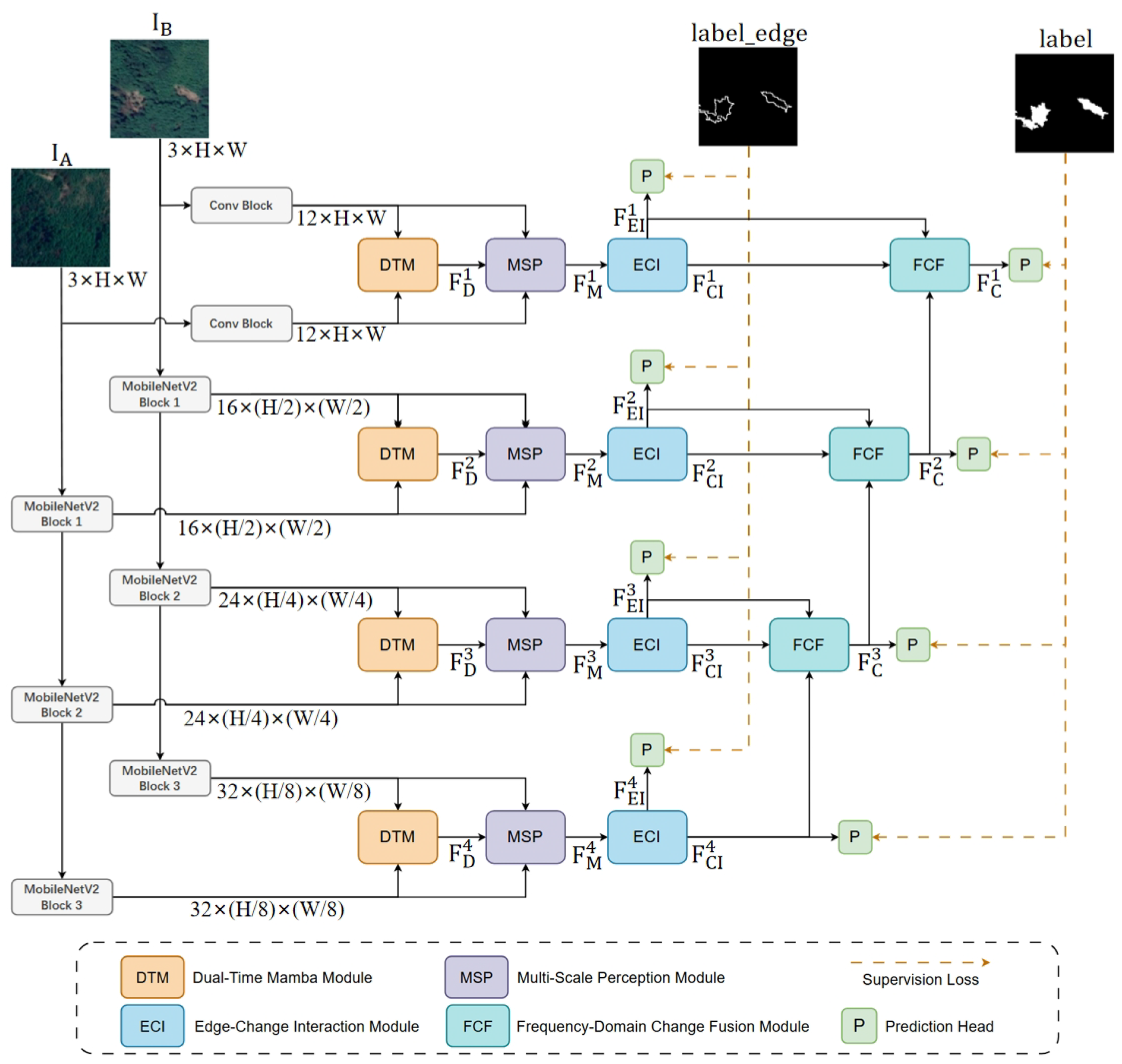
Figure 1. The overall architecture of the proposed MSMCD model.
Remotesensing 18 00108 g001
Figure 2. Illustration of the proposed DTM module.
Remotesensing 18 00108 g002
Figure 3. Illustration of the proposed MSP Module.
Remotesensing 18 00108 g003
Figure 4. Illustration of the proposed ECI module.
Remotesensing 18 00108 g004
Figure 5. Illustration of the proposed FCF module.
Remotesensing 18 00108 g005
Figure 6. TGRM-CD dataset: (a) T1 image. (b) T2 image. (c) Ground truth.
Remotesensing 18 00108 g006
Figure 7. Visualization part 1 of change detection results on the GVLM-CD dataset. (a) T1 image; (b) T2 image; (c) ground truth; (d) FC-EF; (e) FC-Siam-Diff; (f) FC-Siam-Conc; (g) IFNet; (h) SNUNet; (i) ISDANet; (j) BIT; (k) ChangeFormer; (l) MSMCD (Ours). Legend: TP in white, TN in black, FP in red, and FN in green.
Remotesensing 18 00108 g007
Figure 8. Visualization part 2 of change detection results on the GVLM-CD dataset. (a) T1 image; (b) T2 image; (c) ground truth; (d) MSCANet; (e) Paformer; (f) ACABFNet; (g) RS-Mamba; (h) ChangeMamba; (i) CDMamba; (j) MF-VMamba; (k) MSMCD (Ours). Legend: TP in white, TN in black, FP in red, and FN in green.
Remotesensing 18 00108 g008
Figure 9. Visualization part 1 of change detection results on the WHU-CD dataset. (a) T1 image; (b) T2 image; (c) ground truth; (d) FC-EF; (e) FC-Siam-Diff; (f) FC-Siam-Conc; (g) IFNet; (h) SNUNet; (i) ISDANet; (j) BIT; (k) ChangeFormer; (l) MSMCD (Ours). Legend: TP in white, TN in black, FP in red, and FN in green.
Remotesensing 18 00108 g009
Figure 10. Visualization part 2 of change detection results on the WHU-CD dataset. (a) T1 image; (b) T2 image; (c) ground truth; (d) MSCANet; (e) Paformer; (f) ACABFNet; (g) RS-Mamba; (h) ChangeMamba; (i) CDMamba; (j) MF-VMamba; (k) MSMCD (Ours). Legend: TP in white, TN in black, FP in red, and FN in green.
Remotesensing 18 00108 g010
Figure 11. Visualization part 1 of change detection results on the TGRM-CD dataset. (a) T1 image; (b) T2 image; (c) ground truth; (d) FC-EF; (e) FC-Siam-Diff; (f) FC-Siam-Conc; (g) IFNet; (h) SNUNet; (i) ISDANet; (j) BIT; (k) ChangeFormer; (l) MSMCD (Ours). Legend: TP in white, TN in black, FP in red, and FN in green.
Remotesensing 18 00108 g011
Figure 12. Visualization part 2 of change detection results on the TGRM-CD dataset. (a) T1 image; (b) T2 image; (c) ground truth; (d) MSCANet; (e) Paformer; (f) ACABFNet; (g) RS-Mamba; (h) ChangeMamba; (i) CDMamba; (j) MF-VMamba; (k) MSMCD (Ours). Legend: TP in white, TN in black, FP in red, and FN in green.
Remotesensing 18 00108 g012
Figure 13. Visualization of ablation study results for model components on the GVLM-CD dataset: (a) T1 image; (b) T2 image; (c) ground truth; (d) MSMCD without the DTM module; (e) MSMCD without the MSP module; (f) MSMCD without the ECI module; (g) MSMCD without the FCF module; (h) MSMCD (full model). Legend: TP in white, TN in black, FP in red, and FN in green.
Remotesensing 18 00108 g013
Table 1. Quantitative comparisons of IoU, F1, Pre, and Rec on GVLM-CD and WHU-CD datasets.
MethodGVLM-CDWHU-CD
IoU F1 Pre. Rec. IoU F1 Pre. Rec.
FC-EF76.4786.6587.4485.9078.7088.0888.3187.85
FC-Siam-Diff78.0987.6988.1387.2674.7585.5582.5988.73
FC-Siam-Conc77.8287.5386.1788.9374.3785.2983.4187.28
IFNet78.3087.8387.5388.1278.5988.0193.7382.95
SNUNet77.6887.4488.4286.4877.6187.3988.3786.45
ISDANet78.2887.7889.6486.0683.7491.1691.1191.20
BIT78.4187.9089.5586.3181.2989.7291.8787.59
ChangeFormer77.9687.6087.2687.9879.1888.3989.3087.48
MSCANet78.3087.8387.9787.6980.5789.2492.8185.94
Paformer78.2287.7888.0887.4882.8790.6393.0688.33
ACABFNet78.4187.9088.0087.8078.9288.2291.6285.06
RS-Mamba79.2288.4189.6087.2581.3189.6993.5586.14
ChangeMamba78.8088.1689.2387.0883.6591.0994.5287.91
CDMamba78.4687.9490.1585.8284.1191.3694.0688.82
MF-VMamba79.0888.3289.7986.8983.3090.8993.2788.62
MSMCD (Ours)80.2389.0389.0289.0385.5092.1894.4790.01
Table 2. Quantitative comparisons on TGRM-CD dataset and model complexity.
MethodTGRM-CDComplexity
IoU F1 Pre. Rec. Params
(M)
FLOPs
(G)
FC-EF70.6082.7780.6885.031.33.6
FC-Siam-Diff72.8084.2681.4387.281.34.7
FC-Siam-Conc71.5483.4280.4086.661.55.3
IFNet73.3384.6083.1286.1535.782.3
SNUNet73.2484.5383.2385.9212.054.8
ISDANet75.2485.8685.3386.426.93.5
BIT74.2785.1583.487.143.58.8
ChangeFormer73.9785.0584.9785.1141.0202.8
MSCANet74.8585.5484.1587.1216.414.8
Paformer72.1683.8283.1984.4616.110.9
ACABFNet73.7984.9986.6983.22102.328.3
RS-Mamba74.8285.5884.4986.7227.915.7
ChangeMamba75.3085.7184.8786.9849.925.8
CDMamba75.6685.9985.7686.5211.949.6
MF-VMamba75.2185.3486.1685.3157.825.5
MSMCD (Ours)77.3387.2286.3688.096.19.7
Table 3. Ablation study results of model components on the GVLM-CD dataset.
ComponentIoUF1Pre.Rec.
w/o DTM79.2388.4190.1586.74
w/o MSP79.4888.5788.8188.32
w/o ECI79.9388.8588.3089.41
w/o FCF79.6488.6788.7288.61
Full (Ours)80.2289.0389.0289.03
Table 4. Ablation study of loss weights ( λ 1 , λ 2 ) on the GVLM-CD dataset.
λ 1 λ 2 IoUF1Pre.Rec.
1.00.079.7588.7389.1188.35
0.01.079.4988.5888.3288.83
0.50.580.2289.0389.0289.03
1.00.579.5388.6389.3287.94
0.51.079.8888.8488.4689.22
Disclaimer/Publisher’s Note: The statements, opinions and data contained in all publications are solely those of the individual author(s) and contributor(s) and not of MDPI and/or the editor(s). MDPI and/or the editor(s) disclaim responsibility for any injury to people or property resulting from any ideas, methods, instructions or products referred to in the content.