

Influence of Digital Elevation Model Resolution on the Normalized Stream Length–Gradient Index in Intraplate Regions: A Case Study of the Yangsan Fault, Korea

Abstract
1. Introduction
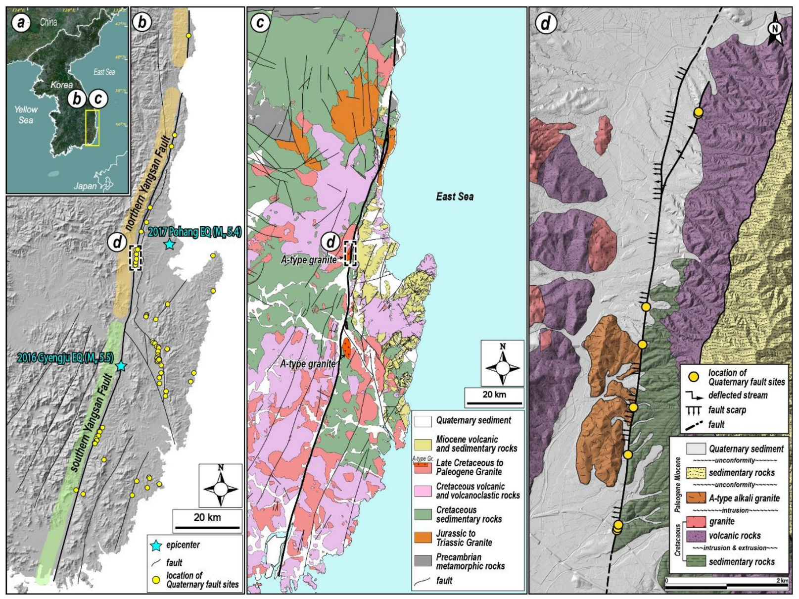
2. Study Area
3. Data and Methods
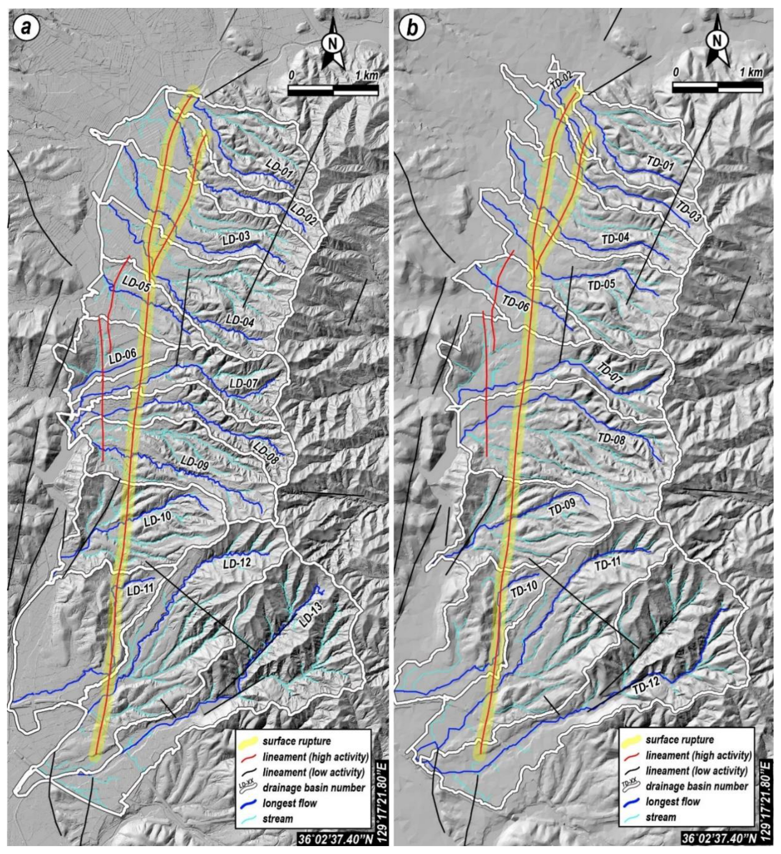
3.1. Data
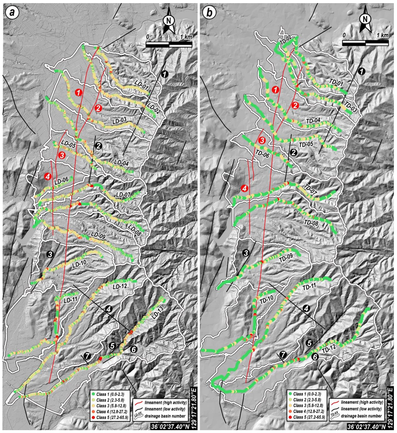
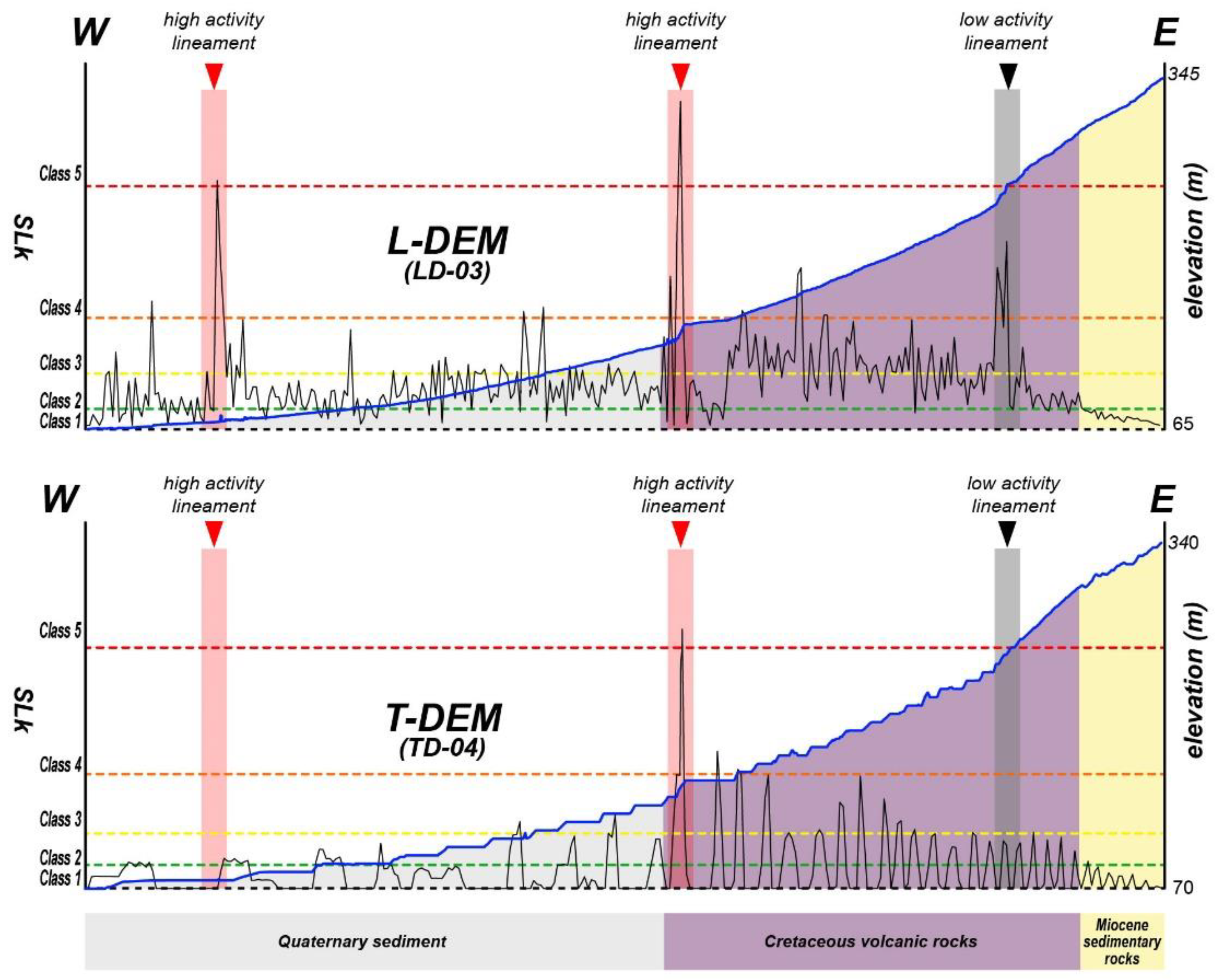
3.2. Normalized Stream Length–Gradient Index
3.3. Fieldwork
4. Results
5. Discussion
6. Conclusions
Author Contributions
Funding
Data Availability Statement
Conflicts of Interest
References
- Bull, W.B.; McFadden, L.D. Tectonic Geomorphology North and South of the Garlock Fault, California. In Geomorphology in Arid Regions, Proceedings of the 8th Annual Geomorphology Symposium, Binghamton, NY, USA, 23–24 September 1977; Doehring, D.O., Ed.; State Univ. New York: Binghamton, NY, USA, 1977; pp. 115–138. [Google Scholar]
- Keller, E.A.; Pinter, N. Active Tectonics: Earthquakes, Uplift, and Landscape; Prentice Hall: New Jersey, NY, USA, 2002. [Google Scholar]
- Hare, P.W.; Gardner, T.W. Geomorphic Indicators of Vertical Neotectonism Along Converging Plate Margins, Nicoya Peninsula, Costa Rica. In Tectonic Geomorphology; Morisawa, M., Hack, J.T., Eds.; Allen & Unwin: Boston, MA, USA, 1985; pp. 75–104. [Google Scholar]
- Strahler, A.N. Hypsometric (Area-Altitude) Analysis of Erosional Topography. Geol. Soc. Am. Bull. 1952, 63, 1117–1142. [Google Scholar] [CrossRef]
- Pike, R.J.; Wilson, S.E. Elevation-Relief Ratio, Hypsometric Integral, and Geomorphic Area-Altitude Analysis. Geol. Soc. Am. Bull. 1971, 82, 1079–1084. [Google Scholar] [CrossRef]
- Mayer, L. Introduction to Quantitative Geomorphology: An Exercise Manual; Prentice Hall: Englewood Cliffs, NJ, USA, 1990. [Google Scholar]
- Bull, W.B. Tectonically Active Landscapes; John Wiley & Sons: Hoboken, NJ, USA, 2011. [Google Scholar]
- Keller, E.A. Investigation of Active Tectonics: Use of Surficial Earth Processes. In Active Tectonics; Wallace, R.E., Ed.; Natl. Acad. Press: Washington, DC, USA, 1986; pp. 136–147. [Google Scholar]
- Hack, J.T. Stream-Profile Analysis and Stream-Gradient Index. J. Res. U.S. Geol. Surv. 1973, 1, 421–429. [Google Scholar]
- Liu, M.; Stein, S. Mid-continental earthquakes: Spatiotemporal occurrences, causes, and hazards. Earth-Sci. Rev. 2016, 162, 364–386. [Google Scholar] [CrossRef]
- Williams, R.T.; Goodwin, L.B.; Sharp, W.D.; Mozley, P.S. Reading a 400,000-year record of earthquake frequency for an intraplate fault. Proc. Natl. Acad. Sci. USA 2017, 114, 4893–4898. [Google Scholar] [CrossRef]
- Kim, T.; Choi, J.H.; Cheon, Y.; Lee, T.-H.; Kim, N.; Lee, H.; Kim, C.-M.; Choi, Y.; Bae, H.; Kim, Y.S.; et al. Correlation of paleoearthquake records at multiple sites along the southern Yangsan Fault, Korea: Insights into rupture scenarios of intraplate strike-slip earthquakes. Tectonophisics 2023, 854, 229817. [Google Scholar] [CrossRef]
- Kim, T.; Lee, H.; Kim, D.E.; Choi, J.-H.; Choi, Y.; Han, M.; Kim, Y.S. Determination of the long-term slip rate of a fault in a slowly deforming region based on a reconstruction of the landform and provenance. Geomorphology 2024, 461, 109286. [Google Scholar] [CrossRef]
- Ha, S.; Kang, H.C.; Lee, S.; Seong, Y.B.; Choi, J.H.; Kim, S.J.; Son, M. Quaternary surface ruptures of the inherited mature Yangsan fault: Implications for intraplate earthquakes in Southeastern Korea. Solid Earth 2025, 16, 197–231. [Google Scholar] [CrossRef]
- Park, S.J. Crustal movement on the Korean Peninsula (I): Determination of the spatial distribution of crustal movement through DEM analysis. J. Korean Geogr. Soc. 2007, 42, 368–387, (In Korean with English Abstract). [Google Scholar]
- Pedrera, A.; Pérez-Peña, J.V.; Galindo-Zaldívar, J.; Azañón, J.M.; Azor, A. Testing the sensitivity of geomorphic indices in areas of low-rate active folding (eastern Betic Cordillera, Spain). Geomorphology 2009, 105, 218–231. [Google Scholar] [CrossRef]
- Kim, D.E.; Kim, C.M.; Cheon, Y.; Choi, J.-H.; Lee, T.-H.; Lee, H.; Choi, Y.; Bae, H.; Kim, T.; Ryoo, C.-R. A case study to find a tectonic landform using geomorphic indices on Keumwang Fault, Korea. In Proceedings of the 2022 Joint Fall Meeting of Geological Sciences and the 77th General Assembly of the Geological Society of Korea, CECO, Changwon, Republic of Korea, 26 October 2022; p. 180. [Google Scholar]
- NGII (National Geographic Information Institute). National Atlas of Korea I; NGII: Suwon, Republic of Korea, 2019. (In Korean)
- Guthrie, R. The catastrophic nature of humans. Nat. Geosci. 2015, 8, 421–422. [Google Scholar] [CrossRef]
- Jeong, A. The Impact of Humans on Desert Landforms in North America: A Case Study of Phoenix, Arizona. J. Korean Geomorphol. Assoc. 2019, 26, 69–85, (In Korean with English Abstract). [Google Scholar] [CrossRef]
- Kim, S.; Lim, H.; Ha, S.; Kim, K.; Son, M. Assessment of Tectonic Activity of Major Faults in Southeastern Korea Using Geomorphic Indices. J. Geol. Soc. Korea 2023, 59, 247–265, (In Korean with English Abstract). [Google Scholar] [CrossRef]
- Lee, C.H.; Seong, Y.B.; Weber, J.; Ha, S.; Kim, D.E.; Yu, B.Y. Topographic metrics for unveiling fault segmentation and tectono-geomorphic evolution with insights into the impact of inherited topography, Ulsan Fault Zone, South Korea. Earth Surf. Dyn. 2024, 12, 1091–1120. [Google Scholar] [CrossRef]
- Azor, A.; Keller, E.A.; Yeats, R.S. Geomorphic Indicators of Active Fold Growth: South Mountain–Oak Ridge Anticline, Ventura Basin, Southern California. Geol. Soc. Am. Bull. 2002, 114, 745–753. [Google Scholar] [CrossRef]
- Silva, P.G.; Goy, J.L.; Zazo, C.; Bardají, T. Fault-Generated Mountain Fronts in Southeast Spain: Geomorphologic Assessment of Tectonic and Seismic Activity. Geomorphology 2003, 50, 203–225. [Google Scholar] [CrossRef]
- El Hamdouni, R.; Irigaray, C.; Fernández, T.; Chacón, J.; Keller, E.A. Assessment of Relative Active Tectonics, Southwest Border of the Sierra Nevada (Southern Spain). Geomorphology 2008, 96, 150–173. [Google Scholar] [CrossRef]
- Khalifa, A.; Çakir, Z.; Owen, L.A.; Kaya, Ş. Evaluation of the Relative Tectonic Activity of the Adıyaman Fault within the Arabian-Anatolian Plate Boundary (Eastern Turkey). Geol. Acta 2019, 17, 1–17. [Google Scholar]
- Viveen, W.; Baby, P.; Hurtado-Enríquez, C. Assessing the Accuracy of Combined DEM-Based Lineament Mapping and the Normalised SL-Index as a Tool for Active Fault Mapping. Tectonophysics 2021, 813, 228942. [Google Scholar] [CrossRef]
- Negi, P.; Goswami, A.; Joshi, G.C. Geomorphic Indices Based Topographic Characterization of Alaknanda Catchment, Western Himalaya Using Spatial Data. Environ. Earth Sci. 2023, 82, 468. [Google Scholar] [CrossRef]
- Sharma, M.; Saraf, A.K. Effect of SRTM resolution on morphometric feature identification using neural network—Self organizing map. Geoinformatica 2010, 14, 241–258. [Google Scholar] [CrossRef]
- Woo, J.-U.; Rhie, J.; Kim, S.; Kang, T.-S.; Kim, K.-H.; Kim, Y. The 2016 Gyeongju Earthquake Sequence Revisited: Aftershock Interactions within a Complex Fault System. Geophys. J. Int. 2019, 217, 58–74. [Google Scholar] [CrossRef]
- Kim, K.-H.; Ree, J.-H.; Kim, Y.; Kim, S.; Kang, S.Y.; Seo, W. Assessing Whether the 2017 Mw 5.4 Pohang Earthquake in South Korea Was an Induced Event. Science 2018, 360, 1007–1009. [Google Scholar] [CrossRef] [PubMed]
- Korea Meteorological Administration (KMA). Earthquake Report of Buan Earthquake (ML 4.8, Jun 12, 2024); Korea Meteorological Administration: Seoul, Republic of Korea, 2024. (In Korean)
- Lee, K.; Lee, J.; Kyung, J.B. A Statistical Analysis of the Seismicity of the Yangsan Fault System. J. Eng. Geol. 1998, 8, 99–114. [Google Scholar]
- Lee, K.; Yang, W.S. Historical Seismicity of Korea. Bull. Seismol. Soc. Am. 2006, 96, 846–855. [Google Scholar] [CrossRef]
- Han, M.; Kim, K.H.; Son, M.; Kang, S.Y.; Park, J.H. Location of Recent Micro-Earthquakes in the Gyeongju Area. Geophys. Geophys. Explor. 2016, 19, 97–104, (In Korean with English Abstract). [Google Scholar] [CrossRef]
- Kim, K.H.; Kang, T.S.; Rhie, J.; Kim, Y.; Park, Y.; Kang, S.Y.; Kim, J. The 12 September 2016 Gyeongju Earthquakes: 2. Temporary Seismic Network for Monitoring Aftershocks. Geosci. J. 2016, 20, 753–757. [Google Scholar] [CrossRef]
- Kim, K.H.; Seo, W.; Han, J.; Kwon, J.; Kang, S.Y.; Ree, J.H.; Liu, K. The 2017 ML 5.4 Pohang Earthquake Sequence, Korea, Recorded by a Dense Seismic Network. Tectonophysics 2020, 774, 228306. [Google Scholar] [CrossRef]
- Lee, J.; Ryoo, Y.; Park, S.C.; Ham, Y.M.; Park, J.S.; Kim, M.S.; Bae, S. Seismicity of the 2016 ML 5.8 Gyeongju Earthquake and Aftershocks in South Korea. Geosci. J. 2018, 22, 433–444. [Google Scholar] [CrossRef]
- Reedman, A.J.; Um, S.H. The Geology of Korea; Geol. Min. Inst. Korea: Ga Jeong, Republic of Korea, 1975; 139p. (In Korean) [Google Scholar]
- Chang, K.H.; Woo, B.G.; Lee, J.H.; Park, S.O.; Yao, A. Cretaceous and Early Cenozoic Stratigraphy and History of Eastern Kyongsang Basin, S. Korea. J. Geol. Soc. Korea 1990, 26, 471–487, (In Korean with English Abstract). [Google Scholar]
- Hwang, B.H.; Lee, J.D.; Yang, K. Petrological Study of the Granitic Rocks Around the Yangsan Fault: Lateral Displacement of the Yangsan Fault. J. Geol. Soc. Korea 2004, 40, 161–178, (In Korean with English Abstract). [Google Scholar]
- Chang, C.J.; Chang, T.W. Structural Movement History of the Yangsan Fault Through High-Stress Analysis. J. Eng. Geol. 1998, 8, 35–49, (In Korean with English Abstract). [Google Scholar]
- Hwang, B.H.; Lee, J.D.; Yang, K.; McWilliams, M. Cenozoic Strike-Slip Displacement Along the Yangsan Fault, Southeast Korean Peninsula. Int. Geol. Rev. 2007, 49, 768–775. [Google Scholar] [CrossRef]
- Hwang, B.H.; McWilliams, M.; Son, M.; Yang, K. Tectonic Implication of A-Type Granites Across the Yangsan Fault, Gigye and Gyeongju Areas, Southeast Korean Peninsula. Int. Geol. Rev. 2007, 49, 1094–1102. [Google Scholar] [CrossRef]
- Cheon, Y.; Ha, S.; Lee, S.; Cho, H.; Son, M. Deformation Features and History of the Yangsan Fault Zone in the Eonyang-Gyeongju Area, SE Korea. J. Geol. Soc. Korea 2017, 53, 95–114, (In Korean with English Abstract). [Google Scholar] [CrossRef]
- Cheon, Y.; Cho, H.; Ha, S.; Kang, H.-C.; Kim, J.-S.; Son, M. Tectonically Controlled Multiple Stages of Deformation Along the Yangsan Fault Zone, SE Korea, Since Late Cretaceous. J. Asian Sci. 2019, 170, 188–207. [Google Scholar] [CrossRef]
- Kim, H.J.; Moon, S.; Jou, H.T.; Lee, G.H.; Yoo, D.G.; Lee, S.H.; Kim, K.H. The Offshore Yangsan Fault Activity in the Quaternary, SE Korea: Analysis of High-Resolution Seismic Profiles. Tectonophysics 2016, 693, 85–95. [Google Scholar] [CrossRef]
- Cheon, Y.; Choi, J.-H.; Choi, Y.; Bae, H.; Han, K.-H.; Son, M.; Choi, S.-J.; Ryoo, C.-R. Understanding the Distribution and Internal Structure of the Main Core of the Yangsan Fault Zone: Current Trends and Future Work. J. Geol. Soc. Korea 2020, 56, 619–640, (In Korean with English Abstract). [Google Scholar] [CrossRef]
- Ryoo, C.-R.; Lee, B.-J.; Cho, D.-L.; Chwae, U.-C.; Choi, S.-J.; Kim, J.-Y. Quaternary Fault of Dangu-ri in Gyeongju Gangdong-myeon: Byeokgye Fault. In Proceedings of the Korean Society of Economic and Environmental Geology/The Korean Society of Mineral and Energy Resources Engineers/Korean Society of Earth and Exploration Geophysicists, Spring Joint Conference, Chungnam National Univ., Daejeon, Republic of Korea, 14 April 1999; p. 334. [Google Scholar]
- Lee, J.; Rezaei, S.; Hong, Y.; Choi, J.-H.; Choi, W.-H.; Rhee, K.-W.; Kim, Y.-S. Quaternary Fault Analysis Through a Trench Investigation on the Northern Extension of the Yangsan Fault at Dangu-ri, Gyungju-si, Gyeongsangbuk-do. J. Geol. Soc. Korea 2015, 51, 471–485, (In Korean with English Abstract). [Google Scholar] [CrossRef]
- Song, Y.; Ha, S.; Lee, S.; Kang, H.-C.; Choi, J.-H.; Son, M. Quaternary Structural Characteristics and Paleoseismic Interpretation of the Yangsan Fault at Dangu-ri, Gyeongju-si, SE Korea, Through Trench Survey. J. Geol. Soc. Korea 2020, 56, 155–173, (In Korean with English Abstract). [Google Scholar] [CrossRef]
- Ha, S.; Son, M.; Seong, Y.B. Active Fault Trace Identification Using a LiDAR High-Resolution DEM: A Case Study of the Central Yangsan Fault, Korea. Remote Sens. 2022, 14, 4838. [Google Scholar] [CrossRef]
- Naik, S.P.; Rockwell, T.K.; Jeong, S.H.; Kim, Y.S.; Shin, H.C.; Choi, J.H.; Son, M. Evidence for Large Holocene Earthquakes Along the Yangsan Fault in the SE Korean Peninsula Revealed in Three-Dimensional Paleoseismic Trenches. Geol. Soc. Am. Bull. 2024, 137, 427–446. [Google Scholar] [CrossRef]
- Oh, J.-S.; Kim, D.E. Lineament Extraction and Its Comparison Using DEMs based on LiDAR, Digital Topographic Map, and Aerial Photo in the Central Segment of Yangsan Fault. J. Korean Geomorphol. Soc. 2019, 54, 507–525, (In Korean with English Abstract). [Google Scholar]
- Woo, J.Y.; Koo, J.H.; Hong, C.H.; Kim, T.H. A Study on Interpolation Methods and Size of Grid to the Topographical Characteristics for the Construction of DEM (Digital Elevation Model). J. Korea Spat. Inf. Syst. Soc. 2001, 3, 5–19, (In Korean with English Abstract). [Google Scholar]
- Bull, W.B. Tectonic Geomorphology of Mountains: A New Approach to Paleoseismology; John Wiley & Sons: Hoboken, NJ, USA, 2008. [Google Scholar]
- Hack, J.T. Studies of Longitudinal Stream Profiles in Virginia and Maryland; U.S. Government Printing Office: Washington, DC, USA, 1957; Volume 294. [Google Scholar]
- Viveen, W.; Van Balen, R.T.; Schoorl, J.M.; Veldkamp, A.; Temme, A.J.A.M.; Vidal-Romani, J.R. Assessment of Recent Tectonic Activity on the NW Iberian Atlantic Margin by Means of Geomorphic Indices and Field Studies of the Lower Miño River Terraces. Tectonophysics 2012, 544, 13–30. [Google Scholar] [CrossRef]
- Pérez-Peña, J.V.; Azañón, J.M.; Azor, A.; Delgado, J.; González-Lodeiro, F. Spatial Analysis of Stream Power Using GIS: SLk Anomaly Maps. Earth Surf. Process. Landforms 2009, 34, 16–25. [Google Scholar] [CrossRef]
- Wu, L.; Xiao, A.; Yang, S. Impact of Wind Erosion on Detecting Active Tectonics from Geomorphic Indexes in Extremely Arid Areas: A Case Study from the Hero Range, Qaidam Basin, NW China. Geomorphology 2014, 224, 39–54. [Google Scholar] [CrossRef]
- Font, M.; Amorese, D.; Lagarde, J.L. DEM and GIS Analysis of the Stream Gradient Index to Evaluate Effects of Tectonics: The Normandy Intraplate Area (NW France). Geomorphology 2010, 119, 172–180. [Google Scholar] [CrossRef]
- Ferrater, M.; Booth-Rea, G.; Pérez-Peña, J.V.; Azañón, J.M.; Giaconia, F.; Masana, E. From Extension to Transpression: Quaternary Reorganization of an Extensional-Related Drainage Network by the Alhama de Murcia Strike-Slip Fault (Eastern Betics). Tectonophysics 2015, 663, 33–47. [Google Scholar] [CrossRef]
- Burbank, D.W.; Anderson, R.S. Geomorphic Markers. In Tectonic Geomorphology; Blackwell Publishing: Malden, MA, USA, 2001; pp. 13–32. [Google Scholar]
- Kim, S.-W.; Choi, E.-K.; Lee, Y.-H. Rock Mass Classification of Tertiary Unconsolidated Sedimentary Rocks In Pohang Area. In Proceedings of the Korean Geotechnical Society Spring National Conference, Incheon Univ., Gyeonggi, Republic of Korea, 27 March 2009; p. 999, (In Korean with English Abstract). [Google Scholar]
- Vaze, J.; Teng, J.; Spencer, G. Impact of DEM Accuracy and Resolution on Topographic Indices. Environ. Model. Softw. 2010, 25, 1086–1098. [Google Scholar] [CrossRef]
- Dávila-Hernández, S.; González-Trinidad, J.; Júnez-Ferreira, H.E.; Bautista-Capetillo, C.F.; Morales de Ávila, H.; Cázares Escareño, J.; López-Baltazar, E.A. Effects of the Digital Elevation Model and Hydrological Processing Algorithms on the Geomorphological Parameterization. Water 2022, 14, 2363. [Google Scholar] [CrossRef]
- Chang, K.T.; Tsai, B.W. The Effect of DEM Resolution on Slope and Aspect Mapping. Cartogr. Geogr. Inf. Syst. 1991, 18, 69–77. [Google Scholar] [CrossRef]
- Troiani, F.; Della Seta, M. The Use of the Stream Length–Gradient Index in Morphotectonic Analysis of Small Catchments: A Case Study from Central Italy. Geomorphology 2008, 102, 159–168. [Google Scholar] [CrossRef]


| Observation date | 8 December 2017 (20 strips) |
| 12 December 2017 (2 strips) | |
| 14 December 2017 (26 strips) | |
| 22 December 2017 (14 strips) | |
| 27 December 2017 (22 strips) | |
| 1 January 2018 (27 strips) | |
| 2 January 2018 (19 strips) | |
| # stripsr (ea) | 124 |
| Flying speed (km/h) | 325 |
| Flying altitude (m) | 830–1193 |
| Scan frequency (kHz) | 200 |
| Swath width (m) | 1300 |
| Laser return points (ea) | 1,856,096,462 |
| Ground point remained (ea) | 317,989,564 |
| Point density (points/m2) | 17.23–26.53 (avg. 21.28) |
| Ground point density (points/m2) | 3.07–4.36 (avg. 3.64) |
| Vertical precision (cm) | 1.2–15.7 (avg. 8.2) |
Disclaimer/Publisher’s Note: The statements, opinions and data contained in all publications are solely those of the individual author(s) and contributor(s) and not of MDPI and/or the editor(s). MDPI and/or the editor(s) disclaim responsibility for any injury to people or property resulting from any ideas, methods, instructions or products referred to in the content. |
© 2025 by the authors. Licensee MDPI, Basel, Switzerland. This article is an open access article distributed under the terms and conditions of the Creative Commons Attribution (CC BY) license (https://creativecommons.org/licenses/by/4.0/).
Share and Cite
Lim, H.; Ha, S.; Kim, S.; Kang, H.-C.; Son, M. Influence of Digital Elevation Model Resolution on the Normalized Stream Length–Gradient Index in Intraplate Regions: A Case Study of the Yangsan Fault, Korea. Remote Sens. 2025, 17, 1638. https://doi.org/10.3390/rs17091638
Lim H, Ha S, Kim S, Kang H-C, Son M. Influence of Digital Elevation Model Resolution on the Normalized Stream Length–Gradient Index in Intraplate Regions: A Case Study of the Yangsan Fault, Korea. Remote Sensing. 2025; 17(9):1638. https://doi.org/10.3390/rs17091638
Chicago/Turabian StyleLim, Hyunjee, Sangmin Ha, Sohee Kim, Hee-Cheol Kang, and Moon Son. 2025. "Influence of Digital Elevation Model Resolution on the Normalized Stream Length–Gradient Index in Intraplate Regions: A Case Study of the Yangsan Fault, Korea" Remote Sensing 17, no. 9: 1638. https://doi.org/10.3390/rs17091638
APA StyleLim, H., Ha, S., Kim, S., Kang, H.-C., & Son, M. (2025). Influence of Digital Elevation Model Resolution on the Normalized Stream Length–Gradient Index in Intraplate Regions: A Case Study of the Yangsan Fault, Korea. Remote Sensing, 17(9), 1638. https://doi.org/10.3390/rs17091638