Abstract
This study utilizes a low-cost Global Navigation Satellite System (GNSS) buoy platform, combined with multi-system GNSS data, to investigate the impact of GNSS signal quality and multipath effects on the accuracy of atmospheric precipitable water vapor (PWV) retrievals. It also explores the methods for oceanic rainfall event forecasting and precipitation prediction based on GNSS-PWV. By analyzing the data quality from various GNSS systems and using the European Centre for Medium-Range Weather Forecasts (ECMWF) ERA5 dataset as a reference, the study assesses the accuracy of PWV retrievals in dynamic marine environments. The results show that the GNSS-derived PWV from the buoy platform is highly consistent with ERA5 data in both trend and characteristics, with an RMSE of 3.8 mm for the difference between GNSS-derived PWV and ERA5 PWV. To enhance rainfall forecasting accuracy, a balanced threshold selection (BTS) method is proposed, significantly improving the balance between the probability of detection (POD) and false alarm rate (FAR). Furthermore, a Random Forest model based on multiple meteorological parameters optimizes precipitation forecasting, especially in reducing false alarms. Additionally, a particle swarm optimization (PSO)-based BP Neural Network model for rainfall prediction achieves high precision, with an R2 of 97.8%, an average absolute error of 0.08 mm, and an RMSE of 0.1 mm. The findings demonstrate the potential of low-cost GNSS buoy for monitoring atmospheric water vapor and short-term rainfall forecasting in dynamic marine environments.
1. Introduction
Oceanic atmospheric water vapor is a crucial component of the global climate system [1], acting as a core driver of air–sea interactions. The energy exchanges associated with its phase transitions significantly impact the formation and development of global atmospheric circulation, the spatial and temporal distribution of precipitation, and the occurrence of extreme weather events such as typhoons [2,3]. Accurate monitoring of atmospheric water vapor over the oceans is not only foundational for improving numerical weather prediction models and enhancing meteorological forecasting capabilities but also a key element in studying climate change and extreme weather events [4,5]. However, due to the unique characteristics of the marine environment, traditional methods of water vapor detection face limitations in oceanic regions. Radio occultation techniques rely on manual launches, which are difficult to meet the continuous observation needs over large areas [6]; microwave radiometers, while offering wide coverage, incur high operational costs and maintenance complexities [7]; and long-term observations using spaceborne microwave radiometers suffer from reduced data accuracy due to drift effects [8]. In recent years, the global navigation satellite system (GNSS) technology has attracted significant attention for its potential application in marine atmospheric water vapor monitoring, owing to its high precision, continuity, and real-time capabilities [9,10].
The PWV inversion technique based on GNSS signals, coupled with buoy platform applications, provides an economically efficient solution to address the shortcomings of traditional methods in marine monitoring. Studies have demonstrated that PWV inversion accuracy from shipborne GNSS observations typically exceeds 2 mm, with high consistency when compared with radiosonde and meteorological reanalysis data from different oceanic regions globally. This technique has been widely utilized for the calibration of spaceborne microwave radiometers and in weather event analysis [11,12]. Furthermore, anchor buoys, with their fixed observation locations, low cost, and advantages in long-term continuous monitoring, have attracted increasing attention in marine meteorological observations in recent years [13,14]. However, multipath effects and signal reflection issues in dynamic marine environments significantly impact the quality of GNSS data, becoming a key factor limiting the accuracy of PWV retrieval. Moreover, while existing studies mainly focus on validating the accuracy of PWV retrieval, research on short-term precipitation forecasting using Buoy GNSS data remains relatively limited.
Previous studies have shown that the temporal variations in precipitable water vapor (PWV) measured by GNSS sensors exhibit a significant correlation with rainfall, particularly before heavy rainfall events, where PWV typically increases significantly and then rapidly decreases [15,16,17,18,19]. Benevides et al. [20] proposed a short-term heavy rainfall forecasting method based on neural networks, which combined GNSS and meteorological data. By processing the data with a nonlinear autoregressive exogenous neural network model, they significantly improved the detection capability for heavy rainfall events and effectively reduced the false alarm rate. Yao et al. [21] developed a short-term precipitation forecasting method that considered the rate of PWV change, the amplitude of PWV variation, and monthly PWV. The method was validated across multiple regions in China, showing an accuracy of 79% to 82% in precipitation rate forecasting, though the false alarm rate remained between 65% and 68%. Additionally, Manandhar et al. [22] proposed a simplified precipitation nowcasting method for tropical regions using the absolute value of PWV and its second derivative, along with seasonal factors. Validation with station data from Singapore and Brazil yielded a true detection rate of 85% to 87%, with a significant reduction in the false alarm rate, which decreased from 37% to 39%. These studies demonstrate that PWV is not only an effective indicator for monitoring the spatial and temporal variations in water vapor but also an important reference parameter for short-term precipitation forecasting. However, existing research has primarily focused on forecasting the occurrence or non-occurrence of rainfall based on PWV and related parameters, with relatively little attention given to precipitation amount prediction. Furthermore, many studies have not considered the application of PWV in oceanic environments. Despite the significant potential of GNSS technology in precipitation forecasting, research on PWV inversion and rainfall prediction based on dynamic GNSS buoys in marine environments is still in its preliminary stages, and a systematic application framework has yet to be established.
Given the current state and limitations of existing research, this study focuses on the use of low-cost GNSS buoy platforms to address data quality analysis and short-term precipitation forecasting in dynamic marine environments. The research primarily investigates the quality of GNSS data in oceanic environments, the accuracy of PWV inversion using multi-system GNSS data, and methods for forecasting precipitation events and predicting rainfall amounts based on PWV. A random forest model incorporating multiple meteorological parameters and a proposed balanced threshold selection (BTS) method is employed for precipitation event forecasting, and the accuracy of different methods in forecasting rainfall events is evaluated. Additionally, a high-precision short-term rainfall prediction model is developed using particle swarm optimization-based BP neural network machine learning techniques, enabling accurate rainfall amount prediction. The prediction accuracy is validated by comparing it with observed rainfall data.
2. Materials and Methods
2.1. Data
The GNSS buoys used in this study were deployed approximately 3 km west of Qianliyan Island, China. The buoy was equipped with UBLOX-M9N GNSS boards and standard antennas, with a market price of around 200 RMB. The observation period was from 23 May to 8 June 2023, during which the experimental site experienced a rainfall event from 26 May to 29 May. The Buoy GNSS data sampling interval was set to 1 s. Simultaneous observations were also conducted at a static reference station located on the island, with the same parameter settings as the Buoy GNSS. The static station on land was equipped with the same GNSS receiver module and antenna as the buoy. The distance between the static station and the Buoy GNSS was approximately 3 km. A map of the study area is shown in Figure 1.

Figure 1.
Study area. (The blue part is the ocean, and the white part is the island).
For regions such as the ocean where direct water vapor detection methods are lacking [23], the European Centre for Medium-Range Weather Forecasts (ECMWF) fifth-generation global climate reanalysis dataset (ERA5) provides a reliable reference for assessing the accuracy of water vapor detection [24]. In this study, while the buoy is equipped with a low-cost GNSS receiver for water vapor detection, the water vapor values calculated from the ERA5 product are used as benchmark data. A comparative analysis is performed to verify the accuracy and reliability of the buoy’s water vapor inversion results. The meteorological data used for short-term precipitation forecasting, including temperature, rainfall, atmospheric pressure, and relative humidity, are obtained from the ECMWF’s fifth-generation reanalysis dataset, with a temporal resolution of 1 h and a spatial resolution of 0.25° × 0.25°. Since the buoy location does not coincide with the grid points of the ERA5 dataset, bilinear interpolation was applied to obtain the meteorological variables at the buoy.
2.2. PWV Retrieval Methods
2.2.1. GNSS Inverse PWV Method
In this study, the precise point positioning (PPP) [25] method was employed to process the GNSS data and derive the PWV, denoted as . The principle behind this approach involves utilizing the GNSS carrier-phase observation equation, where the zenith total delay (ZTD) is treated as an unknown parameter to be solved for [26].
where represents the receiver, denotes the satellite, is the geometric distance from the receiver to the satellite, is the speed of light, is the receiver clock bias, is the satellite clock bias, is the tropospheric mapping function, is the zenith total delay, is the ionospheric delay, is the wavelength of the phase observations, is the phase ambiguity, and represents other errors.
The tropospheric dry delay (zenith hydrostatic delay, ZHD) is calculated using the Saastamoinen model [26]:
where represents the atmospheric pressure, denotes the latitude of the GNSS station, is the ellipsoidal height of the GNSS station, and refers to the zenith hydrostatic delay. The meteorological data were provided by ECMWF. The zenith total delay is subtracted by the dry delay to obtain the zenith wet delay (ZWD). The PWV (), is derived from the GNSS inversion using the empirical equation [27]:
where represents the zenith wet delay, is the gas constant = 461 0.003 Jkg−1K−1); denotes the density of liquid water; = 24 11 Kpa−1, = 3.75 0.03 K2Kpa−1; is the weighted mean temperature of the atmospheric vertical profile.
Due to the fact that the meteorological data provided by the ERA5 dataset is not continuous, as it is derived from different pressure levels, which form a collection of discrete points along the vertical direction, it is necessary to solve it in a discretized form. The formula is as follows:
In the formula, represents the height difference between adjacent pressure levels; is the average of the atmospheric absolute temperatures between adjacent pressure levels; is the average of the atmospheric water vapor pressure between adjacent pressure levels.
The calculation formula for is as follows:
In the formula, represents the atmospheric water vapor pressure (in ); is the specific humidity (in ); is the atmospheric pressure (in ).
The Buoy GNSS data and the static GNSS data used the same data processing strategy. The GNSS data processing strategy used in this study is presented in Table 1.

Table 1.
The GNSS data processing strategy.
2.2.2. PWV Calculation Method Based on ERA5
The formula for calculating using the ERA5 dataset is as follows:
In the equation, represents the density of liquid water, denotes the specific humidity at the layer, is the gravitational acceleration, , represents the pressure difference between the and layers, and indicates the number of pressure layers. The atmospheric pressure and specific humidity can be obtained from the ERA5 dataset.
2.3. Rainfall Event Forecasting Method
2.3.1. Threshold Method for Rainfall Event Forecasting
Yao et al. [21] proposed a three-factor forecasting method that utilizes the PWV value, the change in PWV from adjacent epochs, and its rate of change to predict whether a rainfall event will occur in the near future. In such threshold-based rainfall forecasting methods, if one or more forecast factors exceed their corresponding optimal thresholds, the model predicts the possibility of rainfall occurring within a specified time window. If rainfall actually occurs within that time frame, it is considered an accurate forecast; otherwise, it is considered a false alarm. According to the World Meteorological Organization’s definition of short-term rainfall forecasting [29], this study selects a 12 h forecast window. Consequently, four possible outcomes can arise from the forecast: (1) : the forecast predicts rain, and rainfall occurs within the next 12 h; (2) : the forecast predicts rain, but no rainfall occurs within the next 12 h; (3) : the forecast predicts no rain, but rainfall occurs within the next 12 h; (4) : the forecast predicts no rain, and no rainfall occur within the next 12 h. For the purpose of statistical analysis, a 2 × 2 contingency table is employed to summarize the specific values of , , and .
In this study, the following key performance indicators are primarily used: (1) probability of detection (POD), also referred to as recall, which represents the proportion of accurately forecasted rainfall events among the total true rainfall events. It reflects the model’s ability to correctly identify rainfall events, with higher values indicating better model performance; (2) false alarm rate (FAR), which represents the proportion of erroneously forecasted rainfall events among the total forecasted rainfall events. It reflects the false reporting rate of the model’s rainfall forecasts, with lower values indicating better performance; (3) critical success index (CSI), which is a combined metric of both POD and FAR. Its value ranges from 0 to 1, with higher values indicating better model performance. The calculation formulas for CSI, POD, and FAR are given by Equations (7)–(9).
In threshold-based rainfall forecasting methods, determining the optimal threshold for each forecast factor is one of the key steps. In [30], Li et al. employed the CSI to determine the optimal threshold for each forecast factor, achieving good results in the prediction of heavy rainfall events. However, the optimal thresholds obtained using the CSI method often result in lower POD values, leading to the underreporting of numerous rainfall events. Therefore, the CSI method seems to be more suitable for forecasting heavy rainfall events, with relatively poor applicability to events of varying intensities. The true skill statistic (TSS) method [31], which evaluates model performance by balancing POD and FAR, can still yield high values even in the presence of a high FAR. This suggests that the TSS method may sometimes tend to accept forecasts with higher false alarm rates, potentially leading to an overprediction of rainfall events and affecting the reliability of the forecast results. The calculation formula for is shown in Equation (10).
To address the limitations of the two aforementioned methods, this study proposes the BTS method. The core concept of the BTS method is to maximize the value by considering both POD and FAR simultaneously, thereby optimizing the threshold selection process and avoiding over-reliance on any single metric. In rainfall event forecasting, the method effectively balances the trade-off between missed detections and false alarms, further enhancing the accuracy and reliability of the forecasts. The calculation formula for the BTS value is as follows:
The process for determining the optimal threshold proposed in this study is as follows:
(1) For a given forecast factor, the specific values for each time step within the 12 h preceding the start of each rainfall event (defined as a rainfall event on a given day, e.g., 26 May being a single rainfall event) are calculated. For instance, if a rainfall event occurs at 17:00, the values of the forecast factor are calculated for each full hour from 12 h prior to that time, resulting in a total of 12 values. These 12 values are then sorted from the minimum to the maximum;
(2) From the sorted values of the forecast factor in step (1), the minimum value is selected as the minimum candidate threshold, and the value at the 80% position in the sorted list is selected as the maximum candidate threshold. Then, between the minimum and maximum candidate thresholds, a series of thresholds are selected at fixed intervals (with fixed intervals of 1 mm for PWV, 0.2 mm for PWV increment, and 0.1 mm/h for PWV growth rate) to generate all candidate thresholds for the forecast factor;
(3) Based on the experimental GNSS buoy data, each candidate threshold generated in step (2) is used to forecast the rainfall event. The BTS is then calculated using Equation (8) for each candidate threshold, resulting in a BTS value for each threshold. The threshold corresponding to the maximum BTS value is selected as the optimal threshold for the month, which is then used for forecasting subsequent rainfall events.
2.3.2. Random Forest Method for Rainfall Event Forecasting
This study establishes a short-term rainfall forecasting model based on historical data of rainfall events and their associated meteorological factors using the Random Forest method [32,33]. The specific steps are as follows:
(1) Data collection and integration
PWV data were collected from the GNSS buoy, while precipitation, temperature, atmospheric pressure, and relative humidity at the buoy location were obtained via bilinear interpolation from the surrounding ERA5 data. The temporal resolution is set to hourly, with UTC time used for uniform alignment;
(2) Data cleaning and normalization
The collected data undergo cleaning, including the removal of missing and outlier values. Subsequently, input variables such as temperature, atmospheric pressure, relative humidity, and atmospheric PWV are normalized, with their values scaled between 0 and 1 to reduce the impact of dimensional differences on model training;
(3) Feature variable selection
Based on the target of rainfall event prediction, temperature, pressure, relative humidity, and PWV are selected as input feature variables, while the occurrence of rainfall is treated as the output target variable. These features reflect the relationship between meteorological factors and rainfall amounts;
(4) Validation Set Division and Stratified K-fold Cross-validation
To assess the generalization performance of the model, a 10-fold stratified cross-validation method is employed. The data are divided into a training set (70%), a validation set (15%), and a test set (15%). The dataset consists of 331 non-rain events and 104 rain events, with rain events being notably less frequent. The “train_test_split” method is used to ensure that the test set maintains the same proportion of rain and non-rain events as the original dataset (achieved through the “stratify” parameter).
The remaining 70% of the data are used as the training set. A 10-fold stratified cross-validation is then performed on the training set using the “StratifiedKFold” method. This method ensures that each fold’s training and validation sets contain an appropriate proportion of both rain and non-rain events, which is critical due to the significant class imbalance between rain and non-rain events. Without stratification, traditional K-fold cross-validation could result in certain folds having an insufficient number of samples from one class, adversely affecting the model’s training and evaluation. By using stratified cross-validation, we enhance the model’s ability to learn from both classes and improve its robustness;
(5) Random Forest Model Parameter Optimization
After the cross-validation procedure, the hyperparameters of the Random Forest model are optimized using grid search combined with cross-validation. Key parameters, including the number of decision trees (n_estimators), maximum tree depth (max_depth), minimum samples required to split a node (min_samples_split), and minimum samples required at a leaf node (min_samples_leaf), are determined. These parameters are optimized to balance model complexity and prediction accuracy, thereby enhancing the model’s generalization ability;
(6) Model Training and Final Evaluation
Once the model’s hyperparameters are optimized through cross-validation, the final model is trained using the entire training set, which includes all the data from the 10-fold cross-validation. The independent test set is then used to evaluate the model, ensuring that the test data remains unseen during training and cross-validation. This independent evaluation mitigates the risk of overfitting and ensures that the model’s generalization ability is properly assessed;
(7) Model Performance Evaluation
The trained model is independently validated using the test set data. Metrics such as CSI, POD, and FAR are employed to quantify the accuracy, sensitivity, and false alarm rate of the model’s predictions, providing a comprehensive evaluation of the model’s performance in forecasting rainfall events.
2.4. Rainfall Amount Prediction Method
This study constructs a model for predicting marine rainfall amounts using a backpropagation (BP) neural network [34] optimized by the particle swarm optimization (PSO) algorithm [35], aimed at improving the model’s prediction accuracy and convergence speed. The method includes the following steps:
(1) Data preprocessing
PWV, temperature, atmospheric pressure, and relative humidity data are used as input features, while actual rainfall amounts serve as the target feature. The data are divided into a training set (70%), a validation set (15%), and a test set (15%). The training set is used to train the model, the validation set is used for model tuning and selection, and the test set is used to evaluate the model’s performance. Following data division, the variables are normalized to a [0, 1] range to eliminate the influence of dimensional differences on model performance. The normalization formula is as follows:
where represents the original variable, while and denote the maximum and minimum values of the variable, respectively.
(2) PSO-BP neural network construction
The BP neural network is used to learn the nonlinear mapping relationship between meteorological variables and rainfall amounts. The forward propagation of the neural network is described by the following equation:
where represents the input variables, and are the weights, and are the biases, denotes the output of the hidden layer, and is the final output.
(3) Particle swarm optimization
PSO is used to optimize the initial weights and thresholds of the BP neural network to enhance the model’s performance. The updated equations for the particle velocity and position are as follows:
where represents the current velocity of the particle, denotes the current position of the particle, and are the particle’s historical best position and the global best position, respectively, and are the learning factors, and and are random numbers.
In the particle swarm optimization (PSO) algorithm, the swarm size is set to 50, meaning that 50 particles are used to explore the solution space. These particles iteratively search for the global optimal solution, gradually approaching it with each iteration. The number of iterations for the PSO algorithm is set to 200, ensuring that the algorithm has enough cycles to converge to the optimal solution.
To balance the influence of the individual best position and the global best position on the particle’s movement, the learning factors and are both set to 1.5. These learning factors determine the weight with which each particle moves towards its personal best position and the global best position in every iteration. Random numbers and are uniformly distributed between 0 and 1 in each iteration, which adds randomness to the particle’s position updates. This randomness enhances the diversity of the search process and promotes global exploration.
In the initialization process of the neural network, the initial weights and biases of the BP neural network are randomly initialized within a range of [−0.5, 0.5]. This initialization approach helps avoid symmetry issues within the network and promotes diversity in the learning process, thereby accelerating convergence and improving performance.
(4) Model training and validation
The BP neural network is initialized with the weights and thresholds optimized by PSO, and cross-validation training is performed using the training set data. The error is progressively reduced through the backpropagation algorithm, ultimately capturing the nonlinear relationship between the input variables and rainfall amounts. In the validation phase, the model performance is evaluated using the test set data. The primary evaluation metrics include the following: root mean squared error (RMSE), mean absolute error (MAE), and the coefficient of determination (R2).
3. Results
3.1. Quality Analysis of Ocean Buoy GNSS Observation Data
Due to the widespread presence of water surface reflections in the marine environment, GNSS signals are susceptible to multipath interference during reception, leading to multipath errors that affect the accuracy and signal quality of Buoy GNSS observations. However, adjusting the cut-off angle can effectively reduce the impact of multipath effects. To obtain higher precision PWV data, this study first analyzes the multipath effects of the four major satellite systems—global positioning system (GPS), global navigation satellite system (GLONASS), galileo satellite navigation system (GALILEO), and BeiDou navigation satellite system (BDS)—at various cut-off angles, with the results shown in Table 2. In this study, we use the G-Nut/Anubis [36] software to calculate the multipath errors of GNSS signals. The G-Nut/Anubis v3.10 software is distributed from http://www.gnutsoftware.com. G-Nut/Anubis estimates the multipath error for each satellite by processing the carrier phase and pseudo-range observation data through a linear combination. The multipath values shown in Table 2 represent the mean values for code multipath across all satellites and signals within the specified frequency bands.
Table 2.
Multipath errors of Buoy GNSS (ocean) and static GNSS (land) carrier-phase observation data at different cut-off angles (Unit: mm).
From Table 2, a comparative analysis of the multipath effects across the GPS, GLONASS, GALILEO, and BDS satellite systems in an oceanic environment shows that multipath errors at cut-off angles of 10°, 15°, and 20° are significantly lower than at 5°. For GPS in the ocean environment, within the 5° to 20° range, multipath errors decrease as the cut-off angle increases. Compared to 5°, at 10°, the error is reduced by 6.5%, and at 15° and 20°, the reductions are 19.59%. This suggests that GPS is more sensitive to cut-off changes, with higher errors at lower angles due to increased surface reflection interference. The GLONASS in the ocean environment follows a similar trend, with multipath errors at 10°, 15°, and 20° being significantly lower than at 5°. Compared to 5°, at 10° the error is reduced by 6.74%, and at 15° and 20°, the reductions are 18.64% and 18.71%, respectively. However, the GLONASS G2 observation shows higher multipath errors at lower cut-off angles compared to other components. The GALILEO in the ocean environment shows the best resistance to multipath effects, with smaller error reductions across cut-off angles. Compared to 5°, at 10° the error is reduced by 7.21%, and at 15° and 20°, the reductions are 20.34%. Notably, GALILEO E5a and E5b observations demonstrate minimal error fluctuations, indicating greater stability due to advanced signal design. Similarly, the BDS in the ocean environment exhibits significant multipath error reductions compared to 5°, with 6.98% at 10°, and 18.99% at 15° and 20°. BDS B1, B3, and B2 components show strong resistance to multipath interference, suggesting high reliability in marine environments for precise GNSS buoy monitoring. However, for GNSS in land environments, multipath errors significantly decrease. As the cut-off angle increases, the multipath errors in both oceanic and land environments gradually decrease. This is mainly because, at low cut-off angles, the signal reflection phenomenon is more pronounced in oceanic environments. As the cut-off angle increases, the reflected signals in oceanic environments gradually decrease, and the multipath errors become increasingly similar to those of land stations.
In marine environments, Buoy GNSS observation data are often affected by harsh natural conditions and high dynamic characteristics, which may lead to degraded signal quality and frequent data loss-lock phenomena. The complexity of the marine environment (e.g., wave fluctuations, and frequent multipath reflections) directly impacts the efficiency of GNSS data. Analyzing the data validity rate (the ratio between the expected number of observations and the existing number of observations) of various satellite systems at different cut-off angles is essential for evaluating the reliability of buoy systems and optimizing observation strategies. This study analyzes the data validity rate of different satellite systems at various angles, with the results presented in Figure 2.
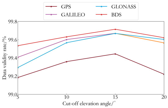
Figure 2.
Data validity rate of Buoy GNSS carrier-phase observation data at different cut-off angles.
From Figure 2, it can be observed that the data validity rate shows only minor variations across different cut-off angles, with differences generally around 0.2%. These small variations have minimal impact on the overall results. The data validity rate tends to be highest at a 15° cut-off angle, with only slight decreases observed at 5° and 20°. Therefore, in the context of this experiment, the choice of cut-off angle has little effect on the data validity rate and processing outcomes.
3.2. PWV Inversion Accuracy Analysis
As the results of previous studies indicate, the impact of different cut-off angles on multipath effects and data validity rate is significant, further affecting the accuracy of GNSS-based PWV inversion. Due to the complexity of the marine buoy environment, the quality and stability of GNSS signals are directly related to the reliability of PWV inversion.
The results in [23] show that, in areas such as the ocean surface where direct water vapor measurements are unavailable, the ERA5 model can serve as a reference value, indirectly reflecting the accuracy of water vapor detection. Therefore, in this study, the PWV values from the ERA5 model are used as a reference to analyze the accuracy of PWV inversions from the Buoy GNSS and static GNSS stations at different cut-off angles. The statistical results of the difference between the PWV obtained from the Buoy GNSS/static GNSS station and the ERA5 PWV are shown in Table 3.
Table 3.
Accuracy analysis of PWV inversion from Buoy GNSS and static GNSS stations at different cut-off angles (Unit: mm).
From Table 3, it can be observed that the accuracy of PWV inversion from the Buoy GNSS is lower than that from the static GNSS station, reflecting the greater impact of the dynamic marine environment on the buoy, including multipath effects and antenna dynamics. However, the accuracy of the Buoy GNSS was found to be better than 4.6 mm within the 10° to 20° cut-off angle range under the conditions tested. As the cut-off angle increases, the accuracy of PWV inversion from the buoy changes, with RMSE decreasing from 5.2 mm at 5° to 3.8 mm at 15°, before slightly rising to 4.0 mm at 20°. This trend is consistent with the influence of multipath effects and signal quality. At 20°, the slight decrease in accuracy may be due to fewer visible satellites and antenna limitations. For the static GNSS station, the variation in PWV inversion accuracy across different cut-off angles is smaller, with RMSE ranging from 3.2 mm at 5° to 2.8 mm at 15°, and slightly rising to 2.9 mm at 20°. The stable environment of the static station appears to result in higher overall accuracy with less sensitivity to changes in the cut-off angle, as observed in this experiment. In this study, the Buoy GNSS shows more significant sensitivity to cut-off angle, with moderate angles (10° and 15°) providing the best accuracy. The static GNSS station, with its stable environment, maintains higher overall accuracy with minimal variation due to cut-off angle changes.
Based on the Douglas Sea Scale [37], we classified sea states according to the significant wave height (SWH) at the buoy location, with the SWH data obtained from the ERA5 dataset. To assess the robustness of the GNSS buoy-based PWV retrieval under varying oceanic conditions, we analyzed the RMSE between GNSS-derived PWV and ERA5 PWV across different sea states. The experiment was conducted with a 15° elevation cutoff angle to ensure that only signals from sufficiently high satellites were considered. The results are shown in Table 4.
Table 4.
RMSE of GNSS and ERA5 PWV under different ocean conditions.
As shown in Table 4, the RMSE increases with deteriorating sea conditions, from 0.82 mm under calm conditions (Sea State 2) to 3.93 mm under rougher conditions (Sea State 4). Despite the performance degradation, the buoy system was still able to output valid data under high sea states, which suggests a level of operational resilience. This preliminary result demonstrates the method’s potential value in monitoring marine atmospheric moisture even during adverse weather, although further validation under extreme conditions (e.g., storms, typhoons) remains necessary.
Building on the previous research findings, this study uses GNSS data at a cut-off angle of 15° for PWV inversion and compares its trend with the ERA5 model PWV, as shown in Figure 3.
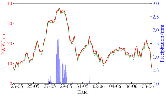
Figure 3.
Comparison of PWV inversion from the Buoy GNSS and ERA5 model PWV.
As shown in Figure 3, the PWV inverted from the Buoy GNSS closely matches the PWV from the ERA5 model in terms of overall trend, accurately reflecting the primary variations in atmospheric water vapor during the observed period. Both datasets show a high degree of synchronization in the timing of peak and trough values, as well as in the trend of changes, indicating that the Buoy GNSS has high accuracy and reliability in capturing atmospheric water vapor dynamics. Furthermore, the GNSS inversion results, with their high temporal resolution, are more capable of detecting localized and short-term water vapor changes, whereas the ERA5 model PWV reflects the variations in large-scale meteorological fields.
3.3. Analysis of the Relationship Between Marine PWV and Rainfall
To explore the potential of applying PWV data in rainfall analysis, the relationship between PWV and precipitation during a selected rainfall event was examined, as shown in Figure 3. During the concentrated rainfall period (from 17:00 on 26 May to 04:00 on 29 May), the variation in precipitation generally corresponds to the trend of PWV changes, with a Pearson correlation coefficient of 0.68.
As shown in Figure 3, during the experiment, the first rainfall event occurred at 07:00 on 25 May, at which point the PWV reached a peak value. Subsequently, as rainfall occurred, the PWV gradually decreased, reflecting the depletion of atmospheric water vapor due to rainfall. At 23:00 on 25 May, the PWV spiked to 38.8 mm, followed by rainfall, during which the PWV fluctuated. This fluctuation may be due to the dynamic balance between water vapor supply and consumption during the rainfall process. As the rainfall intensity decreased, the PWV gradually dropped and returned to normal levels. Around 19:00 on 27 May, the rainfall intensity rapidly increased, causing the PWV to rise quickly, reaching a peak value when the rainfall amount was maximal. Afterward, as the rainfall diminished, the PWV gradually decreased.
Overall, the trend in PWV changes closely mirrors the occurrence and intensity changes in rainfall. Typically, prior to rainfall, the PWV shows a gradual increase. Once it peaks, rainfall begins, and during the rainfall, the PWV fluctuates, likely due to the interplay between water vapor consumption and continuous water vapor transport. After the rainfall ends, the PWV significantly drops and gradually returns to lower levels. The observed pattern suggests that the trend in PWV changes may be a useful precursor to the occurrence of rainfall during concentrated rainfall events, especially during concentrated rainfall events, where the synchronization between the PWV peak and precipitation further validates the crucial role of GNSS-inverted PWV in monitoring short-term rainfall.
However, it is important to note that high PWV values do not always result in rainfall, and several PWV peaks occurred without corresponding precipitation. Therefore, while GNSS-derived PWV shows a degree of co-variability with rainfall during this event, it cannot be used as a sole predictor of precipitation. This analysis is limited to a single event, and broader conclusions require more extensive, multi-event studies incorporating additional meteorological variables.
3.4. Rainfall Event Forecasting Analysis Based on Optimal Threshold
Before forecasting rainfall events, the optimal threshold must first be determined. In this section, the optimal threshold is calculated following the method outlined in Section 2.3.1 and compared with the optimal thresholds determined using the TSS and CSI methods. The results are presented in Figure 4 and Table 5.
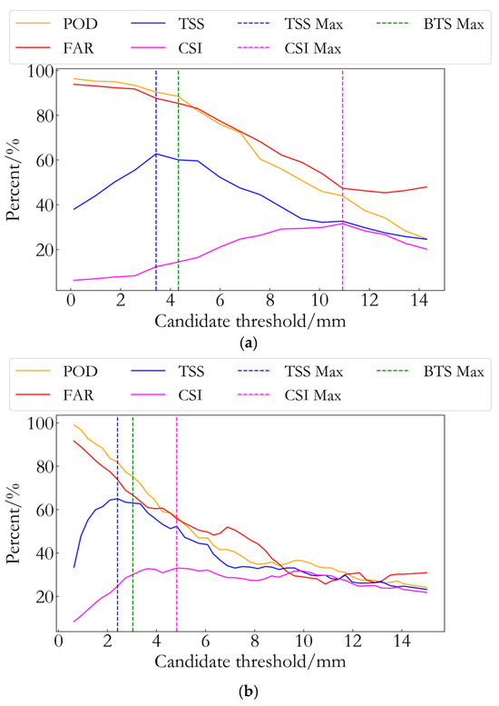
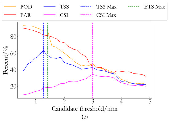
Figure 4.
Candidate thresholds obtained using different methods. (a) Candidate threshold of PWV value. (b) Candidate threshold of PWV increment. (c) Candidate threshold of PWV growth rate.
Table 5.
Optimal thresholds obtained using different methods.
As shown in Figure 4 and Table 5, the CSI reaches its maximum value of 41% at a threshold of 10.1 mm, with POD and FAR values of 46% and 53%, respectively. When the candidate threshold is 3.4 mm, the TSS reaches its maximum value of 63%, with corresponding POD and FAR values of 90% and 87%, respectively. When the candidate threshold is 4.2 mm, the BTS reaches its maximum value of 57%, with corresponding POD and FAR values of 88% and 85%, respectively. In subplot (b) (PWV increment), when the candidate threshold is 4.5 mm, the CSI reaches its maximum value of 33%, with corresponding POD and FAR (highlighted in red boxes) of 58% and 58%, respectively. When the candidate threshold is 2.4 mm, the TSS reaches its maximum value of 65%, with corresponding POD and FAR (highlighted in red boxes) of 82% and 74%, respectively. When the candidate threshold is 3.1 mm, the BTS reaches its maximum value of 54%, with corresponding POD and FAR values of 75% and 66%, respectively. In subplot (c) (PWV growth rate), when the candidate threshold is 2.9 mm/h, the CSI reaches its maximum value of 32%, with corresponding POD and FAR values of 46% and 48%, respectively. When the candidate threshold is 1.3 mm/h, the TSS reaches its maximum value of 53%, with corresponding POD and FAR values of 86% and 82%, respectively. When the candidate threshold is 1.4 mm/h, the BTS reaches its maximum value of 32%, with corresponding POD and FAR values of 87% and 81%, respectively.
From the overall analysis of Figure 4, it can be observed that the optimal threshold determined using the CSI method results in a smaller POD value, leading to a significant number of rainfall events being missed. Therefore, the CSI method seems to be more applicable for forecasting heavy rainfall events. While the optimal threshold determined using the TSS method provides higher POD values, it also results in higher FAR values, leading to a large number of false alarms. In contrast, the optimal threshold determined using the BTS method appears to strike a balance between POD and FAR, maximizing correct detection while minimizing false alarms within the current dataset.
To determine the most appropriate method for selecting the optimal threshold, rainfall forecasting tests were conducted using the optimal thresholds determined by different methods, with the results presented in Table 6.
Table 6.
Performance analysis of different optimal threshold determination schemes.
As shown in Table 6, in the evaluation of different threshold determination methods, the BTS method demonstrates a more balanced advantage. Although its FAR value is slightly higher than that of the TSS method, the difference is minimal. Compared to the CSI method, the BTS method performs better in terms of false alarm rate. Therefore, considering all evaluation metrics, the BTS method is more effective in achieving accurate threshold selection in practical applications. Thus, this study will use the BTS method to determine the optimal threshold.
To explore the rainfall event forecasting performance of different combinations of forecast factors and improve the accuracy of rainfall event predictions, this study designed six different combination strategies (Table 7) and evaluated the performance of these strategies using CSI, POD, and FAR (Table 8).
Table 7.
Six strategies were formed by satisfying different conditions from the three prediction factors.
Table 8.
Performance analysis of six combination strategies.
As shown in Table 8, strategy combination S2 performs exceptionally well across all three evaluation metrics: CSI, POD, and FAR. Notably, it achieves a POD of 89.8%, indicating its superior accuracy in forecasting precipitation events. In contrast, strategy combinations S5 and S6 also perform well in terms of CSI and POD, but their FAR values are slightly higher. The next best is strategy combination S3, which shows good POD performance, though it is slightly weaker in other metrics compared to S2. Combinations S4 and S1 are relatively weaker across all metrics, especially in terms of forecasting accuracy and false alarm rate. Therefore, considering the performance of each strategy, the optimal strategy combination is S2, followed by S5, S6, S3, S4, and S1.
3.5. Rainfall Event Forecasting Based on Multi-Parameter Fusion Random Forest
In Section 2.4, a threshold-based rainfall forecasting method using GNSS water vapor was proposed. Although this method can accurately forecast over 80% of rainfall events, the forecast factors selected are relatively limited. This method typically uses GNSS water vapor time series and its derived parameters (such as PWV increment, PWV growth rate, etc.) to forecast rainfall events, which limits the forecasting effectiveness. The generation of rainfall events is a complex process, with sufficient water vapor being only one of the necessary conditions, not the sole determining factor. It is also significantly correlated with meteorological factors such as temperature, pressure, and relative humidity. Therefore, when using GNSS water vapor for rainfall forecasting, it is essential to further incorporate other atmospheric parameters to develop a more comprehensive forecasting method.
Thus, in this study, a short-term rainfall forecasting model is developed based on the Random Forest method, utilizing meteorological parameters such as PWV, atmospheric temperature (T), dew point temperature (DPT), relative humidity (U), and pressure (P) during rainfall events. The model is used to predict short-term rainfall.
To determine which meteorological parameters should be included in the forecast, the correlations between different parameters and rainfall are first analyzed, with the results shown in Figure 5. The PWV data used for the correlation computation is derived from the Buoy GNSS, while the other meteorological parameters come from the ERA5 dataset. The data cover the period from 23 May to 8 June 2023, with a temporal resolution of 1 h.
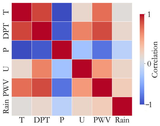
Figure 5.
Correlation analysis of different parameters.
Based on the correlation matrix analysis in Figure 5, the relationships between meteorological parameters reveal their potential roles in rainfall forecasting. The correlation between T (temperature) and DPT (dew point temperature) is close to 0.9, indicating a strong positive correlation between these two variables, reflecting that changes in temperature and humidity are usually synchronized. Since DPT directly reflects the water vapor content in the air, it is particularly sensitive to rainfall prediction. Therefore, removing the T parameter helps reduce model redundancy. PWV shows a strong positive correlation with DPT and T (0.86 and 0.73, respectively), and a weak positive correlation with Rain (0.28). However, during the concentrated rainfall period (from 17:00 on 26 May to 04:00 on 29 May), the correlation between PWV and precipitation reaches 0.68, indicating a close relationship between water vapor and the occurrence of rainfall. Thus, PWV should be included as an important input variable in model training. U (humidity) has a strong correlation with DPT (0.67), but its correlation with rainfall is weaker (0.19). Therefore, humidity can be considered a secondary feature in the model. P (pressure) has strong negative correlations with both T and DPT, indicating that increases in temperature and dew point temperature are typically accompanied by a decrease in atmospheric pressure. However, P has a low correlation with Rain (−0.15), suggesting that pressure plays a relatively minor role in rainfall forecasting. Therefore, in the model, P can be treated as a supplementary feature with lower priority. In summary, when constructing the short-term rainfall forecasting model, this study selects time (annual accumulated days and hours), DPT, PWV, U, and P as input features. Removing temperature (T) will help reduce redundancy and improve the model’s stability and efficiency.
Due to observational limitations, rainfall-related observational data are limited, which makes it uncertain whether the available data can fully meet the requirements for model training. To address this issue, we employed cross-validation to train and validate the model multiple times on different data subsets, evaluating the model’s stability and performance with the limited data. Cross-validation effectively mitigates the risk of overfitting caused by data partitioning bias, thus providing a reliable assessment of the model’s generalization capability. In this study, the model underwent 10 independent training sessions via cross-validation, and the performance of each trained model was evaluated. The validation results are shown in Table 9.
Table 9.
Statistical summary of model performance evaluation metrics from cross-validation.
As shown in Table 9, the results from cross-validation indicate that the model built using the methods and data in this study can adapt well to different data subsets and demonstrates stable predictive capabilities. The model’s accuracy and sensitivity suggest that, under the given data volume and observational conditions, the accuracy of rainfall event prediction is reliable.
During model training, different input meteorological parameters may affect the forecasting performance. This study designs five groups of experiments with different combinations of input parameters, as shown in Table 10.
Table 10.
Six groups of experimental plans with different input parameters.
The RF_TUP, RF_GUP, RF_GTP, and RF_GTU models are designed and compared with the RF_GTUP model to analyze the importance of the PWV, T (DPT), U, and P parameters in rainfall forecasting. The RF_G model is primarily used to investigate the performance of rainfall forecasting when only PWV data are utilized. The results of the different models are shown in Figure 6.
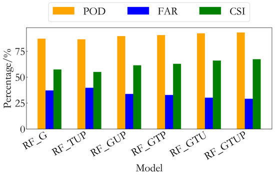
Figure 6.
Performance analysis of different models for rainfall forecasting.
As shown in Figure 6, the RF_GTUP model exhibits the best performance in rainfall forecasting and thus serves as the reference for evaluating the performance of other models. After removing PWV (RF_TUP), the model’s CSI decreased by 18.31%, POD decreased by 7.09%, and FAR increased by 36.77%. In contrast, after removing humidity (U) (RF_GTP), CSI decreased by 6.74%, POD decreased by 2.69%, and FAR increased by 12.71%, indicating that humidity contributes to the model’s performance. Dew point temperature (DPT) and atmospheric pressure (P) have a relatively minor impact on the model. The removal of DPT (RF_GUP) and P (RF_GTU) resulted in changes to CSI by 8.74% and 2.08%, respectively. The model using only PWV data (RF_G) performed significantly worse than RF_GTUP (CSI decreased by 14.70%, POD decreased by 6.44%, and FAR increased by 27.84%), further proving the importance of using multiple meteorological parameters in short-term rainfall forecasting. Based on this analysis, the PWV parameter has the greatest impact on the model’s rainfall forecasting performance, followed by DPT, U, and P.
Compared to traditional threshold-based forecasting methods (CSI MAX method and TSS MAX method), the multi-parameter Random Forest algorithm suggests an improvement in rainfall forecasting performance, particularly in reducing false alarm rates, as observed in the current experiment. This result further highlights the complexity of the rainfall process, which is influenced by multiple meteorological parameters. Therefore, incorporating multiple meteorological parameters in rainfall forecasting may contribute to enhanced accuracy and reliability, as indicated by the results of this study.
3.6. Rainfall Amount Prediction
The random forest method, with its relatively high hit rate and low false alarm rate, shows potential advantages over traditional methods (CSI MAX method and TSS MAX method) in identifying whether a rainfall event will occur. However, given the limited data in this study, further validation is needed to confirm its performance across a broader range of scenarios. However, forecasting rainfall events only addresses the “will it rain?” question. For practical meteorological forecasting, the accurate prediction of rainfall amounts is equally crucial. Compared to the binary classification of rainfall events, predicting rainfall amounts is a more complex task. It not only requires determining the occurrence of a rainfall event but also accurately quantifying the intensity and distribution of rainfall. Therefore, in this study, a rainfall amount prediction model is constructed using a backpropagation (BP) neural network optimized by the particle swarm optimization (PSO) algorithm. The model is applied to predict the amount of rainfall during rainfall events, with the prediction results shown in Figure 7.
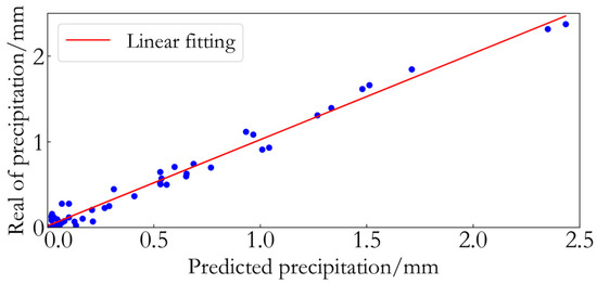
Figure 7.
Comparison analysis of predicted rainfall amount and actual rainfall amount.
As shown in Figure 7, the rainfall amount prediction results based on the PSO-BP neural network method show good consistency with the actual results. The linear fit has an R2 value of 97.8%, indicating a high degree of fit. The fitted line equation is y = 0.98x + 0.02. The predicted values are consistent with the actual values in terms of overall trend, with most points clustered around the fitted line, exhibiting minimal deviation. This suggests that the model is capable of capturing the general variations in rainfall amount. This demonstrates that optimizing the BP neural network with the PSO algorithm significantly enhances the model’s learning ability and generalization performance, allowing it to excel in modeling the nonlinear features of rainfall amounts. Moreover, the slope of the fitted equation is close to 1, and the intercept is near 0, further reflecting the high consistency between the predicted and actual values. These results suggest that this method has the potential for high accuracy in short-term rainfall amount prediction, with good robustness and reliability within the observed dataset, but further testing is needed to confirm these findings across different conditions.
The variations in the predicted rainfall amounts, observed values, and their differences were analyzed, and the results are shown in Figure 8.
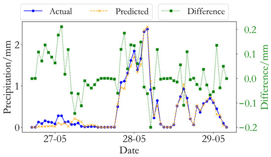
Figure 8.
Analysis of rainfall amount prediction performance.
Figure 8 presents a comparison of the predicted and observed rainfall variations over time. It can be observed that the predicted values exhibit a high level of consistency with the observed rainfall in terms of overall trends, particularly in capturing rainfall peaks and the associated fluctuations. The model reflects the fluctuations in rainfall intensity and is able to reproduce the peak values and decline patterns during heavy rainfall periods (e.g., the rainfall peak on 28 May shown in Figure 8). This suggests that the model demonstrates adaptability in handling complex scenarios involving sudden changes in rainfall. Additionally, during periods of low or no rainfall, the predicted values are typically close to the observed values.
A statistical evaluation of the residuals between observed and predicted precipitation indicates that most differences lie within ±0.19 mm, with larger deviations observed during periods of intense rainfall variability. The MAE and RMSE are 0.08 mm and 0.10 mm, respectively.
However, some discrepancies in predictions can still be observed, particularly in the finer details of the rainfall variations, where the predictions may sometimes be slightly higher or lower than the actual values. These deviations may be related to the nonlinear features of rainfall amounts, the resolution of the input data, or the model’s generalization capabilities. Future improvements could involve incorporating additional input factors or optimizing the model’s structure to further reduce prediction errors and enhance the level of prediction refinement.
4. Discussion
4.1. On the Quality and Representativeness of the Dataset
The results of this study demonstrate that GNSS buoys, even when built with low-cost components, can be utilized to retrieve oceanic precipitable water vapor (PWV) with reasonable accuracy. However, it is important to emphasize that the findings presented are based on a single, short-term observational campaign spanning only 16 days. This inherently limits the representativeness of the dataset and, consequently, the generalizability of the conclusions.
The analysis of GNSS signal quality confirmed that multipath interference—particularly severe in dynamic marine environments—has a non-negligible impact on PWV inversion. Adjusting the satellite elevation cut-off angle was shown to effectively reduce multipath-induced noise, with a 15° cut-off offering the best compromise between signal stability and data availability. While this result aligns with previous studies and supports the feasibility of GNSS-based marine water vapor monitoring, it remains highly context-dependent. Environmental conditions, sea state, antenna installation, and local satellite geometry can all vary substantially across deployments, potentially altering the optimal configuration.
Moreover, the ERA5 reanalysis dataset was used as a reference for evaluating the quality of GNSS-derived PWV. Although ERA5 provides a valuable benchmark for large-scale atmospheric fields, its spatial resolution (0.25° × 0.25°) and temporal granularity may obscure localized variability, particularly over oceanic regions with sparse in situ observations. Therefore, the agreement between buoy-inverted PWV and ERA5 should be interpreted with caution, as it may reflect coarse-scale consistency rather than precise local validation. Furthermore, the study period included only one primary rainfall event, making the dataset insufficient to capture the full spectrum of meteorological variability.
To address these limitations, future research should prioritize long-term deployments (e.g., spanning multiple seasons or a full annual cycle) to enable more robust statistical validation and improve model generalization. Only with extended datasets can the reliability, temporal stability, and transferability of GNSS-based marine PWV monitoring be meaningfully assessed.
4.2. On the Applicability and Limitations of the Forecasting Methods
This study explored two forecasting approaches: a threshold-based method using the proposed BTS scheme, a machine learning approach utilizing random forest classification, and a PSO- BP neural network for rainfall amount prediction. While both methods showed encouraging performance within the bounds of the current dataset, it is essential to recognize that these results are experimental in nature and valid only under the specific conditions of this study.
The BTS method was designed to address the well-known trade-off between POD and FAR in threshold-based rainfall event forecasting. Within the experimental dataset, BTS yielded a more balanced performance than conventional CSI or TSS optimization methods. However, due to the limited number of rainfall events in the dataset, these findings cannot yet be generalized. In operational contexts, the optimal thresholds for PWV, its increment, and its rate of change may vary significantly depending on local climate, seasonal moisture regimes, and synoptic-scale conditions.
The application of machine learning models further highlighted the potential of multi-parameter fusion for short-term rainfall forecasting. The random forest model, incorporating PWV, dew point temperature, relative humidity, and pressure, outperformed threshold-based approaches within the test set. Similarly, the PSO-BP neural network achieved high precision in rainfall amount prediction, with an R2 value of 97.8%. Nevertheless, it must be acknowledged that machine learning models are inherently sensitive to training data volume and distribution. Given the limited temporal coverage and relatively small number of positive rainfall samples, the risk of overfitting is non-negligible. Consequently, these models should be regarded as preliminary demonstrations of feasibility rather than operationally deployable tools.
To establish broader applicability, future studies should focus on employing multi-year, high-frequency GNSS buoy observations across diverse oceanic regions, while incorporating a larger number and variety of rainfall events, including both extreme and stratiform precipitation. It is also essential to conduct out-of-sample validation using unseen temporal windows or independent datasets to rigorously assess model robustness. Moreover, a comparative analysis of model performance under different atmospheric regimes, such as monsoon conditions versus subtropical dry periods, will help elucidate the strengths and limitations of the proposed methods. By systematically addressing these aspects, the current experimental models can be progressively refined into robust and generalizable tools for marine rainfall forecasting.
Although ERA5 data provides high-quality meteorological fields that are valuable for retrospective model development, it is important to note that ERA5 is a reanalysis dataset and cannot be used for real-time forecasting purposes. In this study, the use of ERA5 as both the model input and validation reference was intended as a methodological experiment to demonstrate the feasibility of the proposed model framework. However, this design introduces a limitation: the model is trained and validated within the same data ecosystem, which may lead to overfitting or inflated performance metrics due to implicit data consistency.
For the model to be realistically deployable in operational forecasting scenarios, it must be trained and applied using meteorological inputs derived from forecast-type numerical weather models (NWMs), such as ECMWF HRES or NOAA GFS. These models provide forward-looking, real-time data that are accessible in practical applications and would better reflect the conditions under which a real forecasting system must operate. In future work, we plan to migrate the model training and testing processes to such forecast-based datasets to ensure that the model’s performance remains robust and reliable under real-world data constraints. This transition is critical to bridging the gap between experimental modeling and operational marine rainfall forecasting.
5. Conclusions
This study, based on a low-cost GNSS buoy platform and integrated with multi-system GNSS data, delves into the impact of multipath effects on data quality in dynamic ocean environments, the precision characteristics of GNSS-derived PWV, and the potential applications of PWV in rainfall event forecasting and rainfall amount prediction. The main conclusions are as follows:
(1) Impact of multipath effects and GNSS-derived PWV Accuracy. In dynamic ocean environments, GNSS signals are significantly affected by multipath effects. However, within the cut-off angle range of 10° to 20°, the signal quality and data availability improve significantly, particularly reaching a peak at 15°, where the data availability for all GNSS systems approaches 99.8%. This result indicates that moderate cut-off angles (such as 15°) can significantly enhance signal quality and data availability. Moreover, the RMSE of the difference between GNSS-derived PWV and ERA5 PWV is 3.8 mm with a 15° cut-off angle. Compared to ERA5 reanalysis data, the GNSS-derived PWV from the buoy shows high consistency in overall trends and short-term variations, confirming its effectiveness in monitoring local water vapor changes at high temporal resolution;
(2) A rainfall event forecasting strategy based on the BTS method was proposed. Compared to traditional CSI and TSS methods, the BTS method shows promise in balancing POD and FAR. Additionally, this study explored six different forecasting factor combination strategies to optimize the rainfall event forecasting model. The results suggest that strategy combination S2 performs relatively well in the three evaluation indicators—CSI, POD, and FAR—particularly in improving the accuracy of rainfall event identification;
(3) Impact of meteorological parameters on short-term rainfall forecasting. Through a systematic analysis of the influence of various meteorological parameters on the performance of short-term rainfall forecasting models using the multi-parameter random forest method, the study found that the PWV parameter shows a notable correlation with rainfall, followed by dew point temperature, relative humidity, and pressure. Compared to traditional threshold-based forecasting methods, the multi-parameter Random Forest algorithm showed an improvement in rainfall forecasting performance, particularly in reducing false alarm rates. This emphasizes the importance of integrating multiple meteorological parameters in short-term rainfall forecasting to enhance its accuracy and reliability;
(4) Rainfall amount prediction using particle swarm optimized BP neural network. In rainfall amount prediction, the BP neural network model optimized by PSO successfully captures the nonlinear variations in rainfall amounts. The model shows a high degree of fit between the predicted and actual values, with an R2 value of 97.8%, an MAE of 0.08 mm, and a RMSE of 0.1 mm, reflecting high accuracy and stability. This result suggests that the dynamic correlation between PWV and rainfall may provide useful support for rainfall forecasting, further highlighting the potential advantages of machine learning algorithms in short-term rainfall prediction.
These findings underscore the potential scientific value of the PWV inversion technique based on a low-cost GNSS buoy platform for rainfall forecasting. While the results provide a promising new approach for marine atmospheric process monitoring and short-term weather forecasting, it is important to note that this study is based on a limited dataset and serves as an experimental validation of the method. As such, it should not be considered as a fully operational rainfall forecasting tool at this stage. Future work will focus on long-term data collection and further research to refine the methodology, incorporate additional meteorological factors, and optimize model structures, aiming to enhance the accuracy and broader applicability of rainfall prediction.
Author Contributions
Conceptualization, M.Z. and Y.L.; methodology, M.Z., P.W. and D.Y.; software, P.W. and Z.J.; validation, D.Y., M.L. and D.P.; investigation, Z.H.; data curation, P.W. and Z.J.; writing—original draft preparation, M.Z. and P.W.; writing—review and editing, M.Z., P.W., Z.J. and Y.L.; supervision, Y.L. and D.Y. All authors have read and agreed to the published version of the manuscript.
Funding
This research was funded by the Natural Science Foundation of Shandong Province (ZR2023QD018, ZR2024MD003, ZR2023QD066, ZR2023QB217), the Key R&D Program of Shandong Province, China (2023ZLYS01), the talent research project of Qilu University of Technology (Shandong Academy of Sciences) (2023RCKY050), the Natural Science Foundation of Qingdao (23-2-1-72-zyyd-jch), the Visiting and Training Program for Teachers from Ordinary Undergraduate Universities in Shandong Province Natural Science Foundation of Shandong Province (ZR2024MD003, ZR2023QD066), the Qingdao Marine Science and Technology Innovation Project (23-1-3-hygg-6-hy, 23-1-3-hygg-18-hy), the Major Innovation Project for the Science Education Industry Integration Pilot Project of Qilu University of Technology (Shandong Academy of Sciences) under Grant (2023JBZ03), the Shandong Key Laboratory of Marine Ecological Environment and Disaster Prevention and Mitigation (202405), the Key Laboratory of Aviation-aerospace-ground Cooperative Monitoring and Early Warning of Coal Mining-induced Disasters of Anhui Higher Education Institutes (Anhui University of Science and Technology) (KLAHEI202305).
Data Availability Statement
The GNSS data used in this study can be obtained from the corresponding author upon reasonable request. Meteorological data such as PWV, barometric pressure, precipitation, humidity, and temperature are available for public download on the ECMWF website.
Acknowledgments
We acknowledge Juncheng Wang from the Institute of Oceanographic Instrumentation, Qilu University of Technology (Shandong Academy of Sciences) and Laoshan Laboratory for providing buoy technical guidance and financial support for this article. We would like to thank the organizations that provided the meteorological data.
Conflicts of Interest
The authors declare no conflicts of interest.
Abbreviations
The following abbreviations are used in this manuscript:
| ECMWF | European Centre for Medium-Range Weather Forecasts |
| GNSS | Global navigation satellite system |
| ERA5 | ECMWF fifth-generation global climate reanalysis data |
| BTS | Threshold selection method |
| CSI | Critical success index |
| TSS | True skill statistic |
| POD | Probability of detection |
| FAR | False alarm rate |
| PWV | Precipitable water vapor |
| ZTD | Zenith total delay |
| ZHD | Zenith hydrostatic delay |
| ZWD | Zenith wet delay |
References
- Han, S.; Liu, X.; Jin, X.; Zhang, F.; Zhou, M.; Guo, J. Variations of precipitable water vapor in sandstorm season determined from GNSS data: The case of China’s Wuhai. Earth Planets Space 2023, 75, 126. [Google Scholar] [CrossRef]
- Gong, Y.; Liu, Z.; Chan, P.W.; Hon, K.K. Assimilating GNSS PWV and radiosonde meteorological profiles to improve the PWV and rainfall forecasting performance from the Weather Research and Forecasting (WRF) model over South China. Atmos. Res. 2023, 286, 106677. [Google Scholar] [CrossRef]
- Srivastava, A. Application of GPS PWV for rainfall detection using ERA5 datasets over the Indian IGS locations. J. Earth Syst. Sci. 2024, 133, 60. [Google Scholar] [CrossRef]
- Huang, L.; Lu, D.; Chen, F.; Chen, F.; Zhang, H.; Zhu, G.; Liu, L. A deep learning-based approach for directly retrieving GNSS precipitable water vapor and its application in Typhoon monitoring. IEEE Trans. Geosci. Remote Sens. 2024, 62, 4111712. [Google Scholar] [CrossRef]
- Liu, Y.; Zhao, Q.; Li, Z.; Yao, Y.; Li, X. GNSS-derived PWV and meteorological data for short-term rainfall forecast based on support vector machine. Adv. Space Res. 2022, 70, 992–1003. [Google Scholar] [CrossRef]
- Zhang, Q.; Ye, J.; Zhang, S.; Han, F. Precipitable water vapor retrieval and analysis by multiple data sources: Ground-based GNSS, radio occultation, radiosonde, microwave satellite, and NWP reanalysis data. J. Sens. 2018, 2018, 3428303. [Google Scholar] [CrossRef]
- Fionda, E.; Cadeddu, M.; Mattioli, V.; Pacione, R. Intercomparison of integrated water vapor measurements at high latitudes from co-located and near-located instruments. Remote Sens. 2019, 11, 2130. [Google Scholar] [CrossRef]
- Wang, L.; Hu, X.; Xu, N.; Chen, L. Water vapor retrievals from near-infrared channels of the advanced Medium Resolution Spectral Imager instrument onboard the Fengyun-3D satellite. Adv. Atmos. Sci. 2021, 38, 1351–1366. [Google Scholar] [CrossRef]
- Zhou, M.; Guo, J.; Liu, X.; Hou, R.; Jin, X. Analysis of GNSS-Derived Tropospheric Zenith Non-Hydrostatic Delay Anomaly during Sandstorms in Northern China on 15th March 2021. Remote Sens. 2022, 14, 4678. [Google Scholar] [CrossRef]
- Guo, J.; Hou, R.; Zhou, M.; Jin, X.; Li, G. Detection of Particulate Matter Changes Caused by 2020 California Wildfires Based on GNSS and Radiosonde Station. Remote Sens. 2021, 13, 4557. [Google Scholar] [CrossRef]
- Liu, Y.; Yao, Y.; Zhao, Q. Real-time rainfall nowcast model by combining CAPE and GNSS observations. IEEE Trans. Geosci. Remote Sens. 2022, 60, 4109909. [Google Scholar] [CrossRef]
- Wu, M.; Jin, S.; Li, Z.; Cao, Y.; Ping, F.; Tang, X. High-Precision GNSS PWV and Its Variation Characteristics in China Based on Individual Station Meteorological Data. Remote Sens. 2021, 13, 1296. [Google Scholar] [CrossRef]
- Cao, K.; Luo, X.; Wen, S.; Wei, Y. Research on precipitable water vapor inversion influencing factors of GNSS for offshore mobile platforms. J. Mar. Sci. 2024, 42, 71–80. [Google Scholar]
- Kang, M.; Seol, D. Evaluation of the Appropriateness of High Wind Wave Alert by Comparing the Marine Meteorological Observation Buoy Data. J. Navig. Port Res. 2022, 46, 11–17. [Google Scholar]
- Zhang, K.; Manning, T.; Wu, S.; Rohm, W.; Silcock, D.; Choy, S. Capturing the signature of severe weather events in Australia using GPS measurements. IEEE J. Sel. Top. Appl. Earth Obs. Remote Sens. 2015, 8, 1839–1847. [Google Scholar] [CrossRef]
- Zhao, Q.; Liu, Y.; Ma, X.; Yao, W.; Yao, Y.; Li, X. An improved rainfall forecasting model based on GNSS observations. IEEE Trans. Geosc. Remote Sens. 2020, 58, 4891–4900. [Google Scholar] [CrossRef]
- Zhang, W.; Zhang, H.; Liang, H.; Lou, Y.; Cai, Y.; Cao, Y.; Zhou, Y.; Liu, W. On the suitability of ERA5 in hourly GPS precipitable water vapor retrieval over China. J. Geod. 2019, 93, 1897–1909. [Google Scholar] [CrossRef]
- Li, H.; Wang, X.; Choy, S.; Jiang, C.; Wu, S.; Zhang, J.; Qiu, C.; Zhou, K.; Li, L.; Fu, E.; et al. Detecting heavy rainfall using anomaly-based percentile thresholds of predictors derived from GNSS-PWV. Atmos. Res. 2022, 265, 105912. [Google Scholar] [CrossRef]
- Huang, L.; Mo, Z.; Xie, S.; Liu, L.; Chen, J.; Kang, C.; Wang, S. Spatiotemporal characteristics of GNSS-derived precipitable water vapor during heavy rainfall events in Guilin, China. Satell. Navig. 2021, 2, 13. [Google Scholar] [CrossRef]
- Benevides, P.; Catalao, J.; Nico, G. Neural Network Approach to Forecast Hourly Intense Rainfall Using GNSS Precipitable Water Vapor and Meteorological Sensors. Remote Sens. 2019, 11, 966. [Google Scholar] [CrossRef]
- Yao, Y.; Shan, L.; Zhao, Q. Establishing a method of short-term rainfall forecasting based on GNSS-derived PWV and its application. Sci. Rep. 2017, 7, 12465. [Google Scholar] [CrossRef] [PubMed]
- Manandhar, S.; Lee, Y.H.; Meng, Y.S.; Yuan, F.; Ong, J. GPS-derived PWV for rainfall nowcasting in tropical regions. IEEE Trans. Geosci. Remote Sens. 2018, 56, 4835–4844. [Google Scholar] [CrossRef]
- Huang, L.; Mo, Z.; Liu, L.; Zeng, Z.; Chen, J.; Xiong, S.; He, H. Evaluation of hourly PWV products derived from ERA5 and MERRA-2 over the Tibetan Plateau using ground-based GNSS observations by two enhanced models. Earth Space Sci. 2021, 8, e2020EA001516. [Google Scholar] [CrossRef]
- Wu, Z.; Lu, C.; Han, X.; Zheng, Y.; Wang, B.; Wang, J.; Liu, Y.; Liu, Y. Real-time shipborne multi-GNSS atmospheric water vapor retrieval over the South China Sea. GPS Solut. 2023, 27, 179. [Google Scholar] [CrossRef]
- Kuo, C.Y.; Chiu, K.W.; Chiang, K.W.; Cheng, K.C.; Lin, L.C.; Tseng, H.Z.; Chu, F.Y.; Lan, W.H.; Lin, H.T. High-frequency sea level variations observed by GPS buoys using precise point positioning technique. TAO Terr. Atmos. Ocean. Sci. 2012, 23, 209. [Google Scholar] [CrossRef]
- Saastamoinen, J. Atmospheric correction for the troposphere and stratosphere in radio ranging satellites. Use Artif. Satell. Geod. 1972, 15, 247–251. [Google Scholar]
- Sleem, R.; Abdelfatah, M.; Mousa, K.; El-Fiky, G. A new Egyptian Grid Weighted Mean Temperature (EGWMT) model using hourly ERA5 reanalysis data in GNSS PWV retrieval. Sci. Rep. 2024, 14, 14608. [Google Scholar] [CrossRef]
- Böhm, J.; Werl, B.; Schuh, H. Troposphere mapping functions for GPS and VLBI from ECMWF operational analysis data. J. Geophys. Res. 2006, 111, B02406. [Google Scholar]
- Wang, Y.; Coning, E.D.; Harou, A.; Jacobs, W.; Joe, P.; Nikitina, L.; Roberts, R.; Wang, J.; Wilson, J.; Atencia, A.; et al. Guidelines for Nowcasting Techniques; World Meteorological Organization: Geneva, Switzerland, 2017. [Google Scholar]
- Li, H.; Wang, X.; Wu, S.; Zhang, K.; Chen, X.; Qiu, C.; Zhang, S.; Zhang, J.; Xie, M.; Li, L. Development of an improved model for prediction of short-term heavy precipitation based on GNSS-derived PWV. Remote Sens. 2020, 12, 4101. [Google Scholar] [CrossRef]
- Li, L.; Zhang, K.; Wu, S.; Li, H.; Wang, X.; Hu, A.; Li, W.; Fu, E.; Zhang, M.; Shen, Z. An improved method for rainfall forecast based on GNSS-PWV. Remote Sens. 2022, 14, 4280. [Google Scholar] [CrossRef]
- Yu, P.; Yang, T.; Chen, S.; Kuo, C.; Tseng, H. Comparison of random forests and support vector machine for real-time radar-derived rainfall forecasting. J. Hydrol. 2017, 552, 92–104. [Google Scholar] [CrossRef]
- Pham, L.; Luo, L.; Finley, A. Evaluation of Random Forest for short-term daily streamflow forecast in rainfall and snowmelt driven watersheds. Hydrol. Earth Syst. Sci. Discuss. 2021, 25, 2997–3015. [Google Scholar] [CrossRef]
- Vamsidhar, E.; Varma, K.; Rao, P.; Satapati, R. Prediction of rainfall using backpropagation neural network model. Int. J. Comput. Sci. Eng. 2010, 2, 1119–1121. [Google Scholar]
- Xiao, P.; Guo, B.; Wang, Y.; Xian, Y.; Zhang, F. Research on the Prediction of Infiltration Depth of Xiashu Loess Slopes Based on Particle Swarm Optimized Back Propagation (PSO-BP) Neural Network. Water 2024, 16, 1184. [Google Scholar] [CrossRef]
- Vaclavovic, P.; Dousa, J. G-Nut/Anubis: Open-source tool for multi-GNSS data monitoring with a multipath detection for new signals, frequencies and constellations. In IAG 150 Years: Proceedings of the IAG Scientific Assembly in Postdam, Germany, 1–6 September 2013; Springer International Publishing: Cham, Switzerland, 2015; pp. 775–782. [Google Scholar]
- Owens, E.H. Sea conditions. In Beaches and Coastal Geology; Encyclopedia of Earth Sciences Series; Springer: New York, NY, USA, 1982. [Google Scholar]
Disclaimer/Publisher’s Note: The statements, opinions and data contained in all publications are solely those of the individual author(s) and contributor(s) and not of MDPI and/or the editor(s). MDPI and/or the editor(s) disclaim responsibility for any injury to people or property resulting from any ideas, methods, instructions or products referred to in the content. |
© 2025 by the authors. Licensee MDPI, Basel, Switzerland. This article is an open access article distributed under the terms and conditions of the Creative Commons Attribution (CC BY) license (https://creativecommons.org/licenses/by/4.0/).