Article

Specific Responses to Environmental Factors Cause Discrepancy in the Link Between Solar-Induced Chlorophyll Fluorescence and Transpiration in Three Plantations

1
Key Laboratory of Tree Breeding and Cultivation, National Forestry and Grassland Administration, Research Institute of Forestry, Chinese Academy of Forestry, Beijing 100091, China
2
Henan Xiaolangdi Forest Ecosystem National Observation and Research Station, Jiyuan 454650, China
3
Collaborative Innovation Center of Sustainable Forestry in Southern China, Nanjing Forest University, Nanjing 210037, China
*
Author to whom correspondence should be addressed.
These authors contributed equally to this work.
Remote Sens. 2025, 17(9), 1625; https://doi.org/10.3390/rs17091625
Submission received: 17 March 2025 / Revised: 28 April 2025 / Accepted: 30 April 2025 / Published: 3 May 2025

Abstract

:
Vegetation transpiration (Tr) is crucial for the water cycle, regional water balance, and plant growth but remains challenging to estimate at large scales. Sun-induced chlorophyll fluorescence (SIF) provides a novel method for estimating Tr, but its effectiveness is limited by species specificity, requiring continuous tower-based observations for comprehensive analysis across diverse ecosystems. In this study, SIF and Tr were simultaneously monitored in Chinese cork oak (ring-porous), poplar (diffuse-porous), and arborvitae (non-porous) plantations in northern China, and the SIF–Tr relationship was further analyzed. The results showed that SIF and Tr shared similar diurnal dynamics, although Tr exhibited midday saturation. SIF and Tr were closely correlated, and the correlation strengthened as the temporal scale aggregated. Environmental factors had nonlinear impacts on SIF and Tr. Therefore, the SIF–Tr relationship deteriorated to some extent at midday, with short-term stress reducing the correlation by 0.1–0.23. Compared to the linear empirical model, the inclusion of environmental factors improved the accuracy of SIF-based Tr estimation, increasing the R2 value by 0.12 to 0.37. At the same level of accuracy, the number of environmental variables required was higher at the half-hour scale than at the daily scale. This study demonstrated the species-specific influence of environmental factors on SIF and Tr in different plantations, enhanced the understanding of the SIF–Tr relationship, and provided theoretical and data support for future large-scale Tr predictions using satellite-based SIF.

1. Introduction

Evapotranspiration (ET) is an essential component of the global water cycle and the land surface energy balance [1], with transpiration (Tr) predominating in the evapotranspiration of terrestrial ecosystems [2]. Therefore, accurately estimating vegetation transpiration not only helps in understanding plant water use strategies and guiding forest management [3], but is also crucial for understanding the exchange of carbon, water, and energy between terrestrial ecosystems and the atmosphere [4]. At present, techniques for measuring leaf and individual tree scale transpiration are relatively well-developed, but with the scale up to regional or even global levels, the estimation of transpiration will exhibit uncertainty [5].
At the leaf and individual tree scales, common methods for measuring/estimating transpiration include the gas exchange chamber method, the sap flow method, and the lysimeter method [6]. At the ecosystem scale, the eddy covariance method based on micrometeorology can be used to reliably observe evapotranspiration. The methods for estimating large-scale evapotranspiration using remote sensing techniques are mainly divided into three categories: models based on land surface water or energy balance [7,8], models based on meteorological simplification and mechanistic process [9], and empirical or machine learning models driven by meteorological/optical remote sensing parameters or vegetation indices (VIs) [10]. With the development of spectral observation techniques and retrieval algorithms, it has been found that sun-induced chlorophyll fluorescence (SIF) is directly related to plant physiology. Compared with conventional VIs, SIF contains information on both canopy structure and photosynthetic physiology, potentially enabling a novel approach for Tr estimation [11,12].
SIF is the light signal re-emitted by vegetation after absorbing photosynthetic active radiation (APAR) and is a by-product of photosynthesis. Compared with active fluorescence, SIF is easier to obtain at canopy and larger scales, and has been widely used to indicate early stress of vegetation [13], observe phenology [14] and estimate gross primary productivity [15]. Stomata are the channels through which leaves control the exchange of gas. The physiological relationship between photosynthesis and fluorescence, and the coupling of photosynthesis and transpiration through stomatal behavior, provide a theoretical basis for the relationship between SIF and Tr. At present, research based on different types of terrestrial ecosystems has found correlations between SIF and Tr at multiple temporal and spatial scales [16,17], which have utilized different approaches to retrieve Tr from SIF. The main approaches include linear empirical relationship between SIF and Tr or canopy conductance [18]; machine learning or other statistical regression models with SIF and environmental factors as independent variables [19]; SIF-based estimates of Tr through land surface, meteorological, hydrological and photosynthesis models [20,21,22,23,24]; and the establishment of mechanistic or semi-mechanistic models based on SIF that consider stomatal behavior and carbon-water coupling relationships [25,26,27]. Mechanistic models typically involve significant assumptions and simplifications, with certain parameters being inherently difficult to quantify. Machine learning methods can achieve precise ET inversion without requiring explicit consideration of mechanistic relationships between variables [28]. Alemohammad et al. retrieved latent heat flux using SIF data through an artificial neural network (ANN) approach [19]. Zheng et al. achieved canopy conductance retrieval by combining SIF and photochemical reflectance index using a random forest model [29].
However, the mismatch in spatial and temporal scales of data sources and the variability in the relationship between SIF and Tr will limit the estimation accuracy. The observation intervals and the pixel representative area of satellite SIF are relatively large, which may result in a mixture of different vegetation cover types, leading to a poor match with ground eddy covariance flux data [30]. Ground-based SIF observations have temporal continuity and spatial representativeness [31], which can refine ground observation datasets and provide a suitable choice for thorough analysis of the relationship between SIF and Tr. The temporal scale can influence the relationship between SIF and Tr, with a higher correlation being observed at lower spatiotemporal resolutions [32]. At a detailed temporal scale, the estimation capability of SIF for Tr declined, which could be due to the complex response of the relationship between photosynthesis and transpiration to environmental changes. Moreover, because SIF signals are substantially weaker than background radiance, random noise in high-temporal-resolution measurements can significantly compromise the SIF–Tr relationship. Lu et al. [18] found that vapor pressure deficit (VPD) may affect SIF–Tr, and Shan et al. [26] enhanced the relationship between SIF and stomatal conductance (gc) after incorporating VPD. Similarly, the asynchronous response of SIF and photosynthesis to environmental changes can introduce significant uncertainty when utilizing SIF. Comparing different ecosystems revealed that the correlation between SIF and Tr is higher in croplands and forests, while it is lower in grasslands or sparse woodlands with lower canopy coverage [24]. Overall, the spatiotemporal scale and type of vegetation affect the relationship between SIF and Tr.
Previous research has primarily focused on comparisons between different vegetation functional types, often overlooking the impact of species-specific factors. Compared to croplands, forests have more complex canopy structures and physiological variations, leading to greater inter-species differences in the ability of SIF to estimate Tr. Therefore, refining observations of SIF and Tr for different tree species at high temporal resolution can enhance the understanding of how the relationship responds to environmental factors and improve the capability of SIF in estimating Tr. Based on the differences in water-conducting tissues, woody plants can be categorized into ring-porous, diffuse-porous, and non-porous (tracheid) species. Trees adopt specific coping strategies under drought, which lead to differences in stomatal behavior and water use [33]. We chose Chinese cork oak (Quercus variabilis var. variabilis, ring-porous), poplar (Populus nigra var. italica, diffuse-porous), and arborvitae (Platycladus orientalis, non-porous) plantations to clarify the relationship between SIF and Tr and its response to environmental changes in different forest systems. The aims of this study are (1) to compare the temporal dynamics and patterns of SIF, Tr, and SIF–Tr relationship in three plantations; (2) to analyze the response of the SIF–Tr relationship to environmental factors; and (3) to evaluate Tr model predictability driven by SIF and environmental factors.

2. Materials and Methods

2.1. Study Sites and Measurements

2.1.1. Study Sites

We selected three typical plantation forests, Chinese cork oak, poplar, and arborvitae, located in warm temperate monsoon climate zone of northern China, for field observation. Chinese cork oak plantation (35°01′45″N, 112°28′08″E) and arborvitae plantation (35°11′24″N, 112°35′24″E) are located in Jiyuan City, Henan Province. The soil is primarily composed of brown soil and limestone weathered eluvial brown soil with a high content of gravel. The forests’ ages are 49 years and 33 years, respectively, with average heights of 10.5 m and 8 m. Grewia biloba G. and Vitex negundo L. dominate the under canopy of the Chinese cork oak plantation, while Vitex negundo L. primarily makes up the understory of the arborvitae plantation. In two sites, the litter layer is relatively thick, and herbaceous plants are seldom found. The poplar (34°43′55″N, 115°04′48″E) plantation is located in Shangqiu City, Henan Province, on the old course of the Yellow River, and has sandy, thick soil. The age of poplar plantation is 20 years, the trees’ height averaging 20 m. There are no shrubs in the under canopy of this site, and the herbaceous layer is primarily dominated by Senna tora L.

2.1.2. The Observation of Tower-Based SIF

We used the tower-based automatic spectral observation system AutoSIF-1 (Bergsun Inc., Beijing, China) to observe SIF in Chinese cork oak and poplar plantations. At both sites, the system utilized QE65Pro and QE Pro spectrophotometers (Ocean Optics Inc., Dunedin, FL, USA) with a spectral resolution of 0.31 nm, a sampling interval of 0.155 nm, and a spectral range from 650 to 800 nm. The SIF in the arborvitae plantation was collected by the vegetation canopy fluorescence observation system D-Flox (Agri-SIF Inc., Nanjing, China), which utilized a QE Pro spectrophotometer (Ocean Optics Inc., Dunedin, FL, USA). The resolution and spectral range of all three observation systems can both meet the accuracy requirements for spectral observation during fluorescence retrieval. The instruments were, respectively, set up at the top of the canopy of Chinese cork oak, poplar, and arborvitae plantations at 10 m, 20 m, and 5 m, with the fiber optics located on the south side of the tower to avoid the effects of shadow and obstruction. The “sandwich” method was employed to reduce the observation errors caused by instantaneous fluctuations in radiation [34]. Depending on the radiation conditions, each spectral measurement interval is approximately 3–5 min. We used the Spectral Fitting Method (SFM) algorithm, which is based on the Fraunhofer Line, to retrieve SIF from reflectance for the band around O2-A (760 nm) absorption [35].

2.1.3. Eddy Covariance Flux and Environment Measurements

Eddy covariance systems are used to observe the water vapor flux exchange between the canopy and the atmosphere in each plantation. Eddy covariance systems consist of a three-dimensional sonic anemometer (CSAT3, Campbell Scientific Inc., Logan, UT, USA) and an open-path infrared gas analyzer (LI-7500, LI-COR, Lincoln, NE, USA), operating at a sampling frequency of 10 Hz, with data recorded by a CR5000 data logger. In addition, each site is equipped with an automatic meteorological observation system for continuous monitoring of photosynthetically active radiation (PAR), air temperature (Ta), relative humidity (RH), wind speed (Ws), soil moisture (SM), and precipitation [36]. VPD refers to the difference between the saturation vapor pressure and the actual vapor pressure in the air at a certain temperature [37]. The formula for calculating VPD is
V P D = ( 1 R H / 100 ) × 0.611 × e x p 17.27 × T a 237.3 + T a
VPD represents the vapor pressure deficit (kPa), Ta represents air temperature (°C), and RH denotes relative humidity (%).

2.2. Description of Data Analysis

The analysis of SIF, Tr, and environmental factors in this research is based on data collected daily from 7:00 to 17:30 during the period from 2021 to 2022. We assume that Tr predominantly dominates ET during the observation period. To mitigate the effects of soil evaporation and interception evaporation, we selected data from June to September, when the leaves are fully expanded, the canopy structure is stable, and changes in LAI are relatively small. Additionally, we excluded data from the days of rainfall and the following day.

2.2.1. Acquisition of Vegetation Index

The vegetation index can reflect dynamics in canopy structure, pigments, and physiology, and can be calculated using vegetation reflectance. The formulas for the Normalized Difference Vegetation Index (NDVI) and the MERIS Terrestrial Chlorophyll Index (MTCI) are as follows [38,39]:
N D V I = R N I R R r e d R N I R + R r e d
M T C I = R N I R R r e d e d g e R r e d e d g e R r e d
RNIR, Rred, and Rrededge represent the average vegetation reflectance in the spectral bands of 770–780 nm, 650–660 nm, and 700–710 nm, respectively.
Previous research has found that weather conditions, particularly the state of radiation, can affect leaf photosynthesis and stomatal behavior [40]. We selected clearness index (CI) as the standard for clarify the weather condition, using 0.5 as the threshold to differentiate between sunny days (CI ≥ 0.5) and cloudy days (CI < 0.5) [41]. The calculation process for CI is as follows [42]:
C I = R g R 0
R 0 = R s c × 1 + 0.033 × cos 360 × D O Y 365 × cos θ
In the formula, Rg represents the total solar radiation; R 0 represents extraterrestrial radiation at the top of the atmosphere; Rsc is the solar constant, noted as 1367 W∙m−2; θ is the solar zenith angle.

2.2.2. Canopy Transpiration Estimation and Evaluation

Random Forest model can explore relationships between independent variables and dependent variables [43]. In this study, 66.7% of the SIF, Tr, and environmental factor (including PAR, Ta, VPD, SM, and Ws) observations were allocated to the training dataset (for model calibration), while the remaining 33.3% were assigned to the validation dataset (for performance evaluation). We established separate Random Forest models using the ‘randomForest’ package in R 4.3.3, with SIF and environmental factors at two temporal scales across different plantations as predictors and Tr as the response variable:
T r ~ R F S I F , P A R , T a , V P D , S M , W S
The relative importance of each predictor variable in estimating Tr was quantified using 10-fold cross-validation performed on the training dataset. We ranked them by significance and then sequentially reduced each environmental factor to assess its impact on the accuracy of Tr estimation. Model evaluation was conducted on the validation dataset using the coefficient of determination (R2) and root mean squared error (RMSE) as performance indicators. The calculation formulas are as follows:
R 2 = 1 i = 1 N P i O i 2 i = 1 N O ¯ O i 2
M A E = 1 N i = 1 N P i O i
R M S E = [ N 1 i = 1 N P i O i 2 ] 0.5
P i denotes the predicted Tr from the random forest model applied to the validation dataset; O i represents the observed Tr values in the validation dataset; O ¯ is average of observed values; N is the count of samples.

3. Results

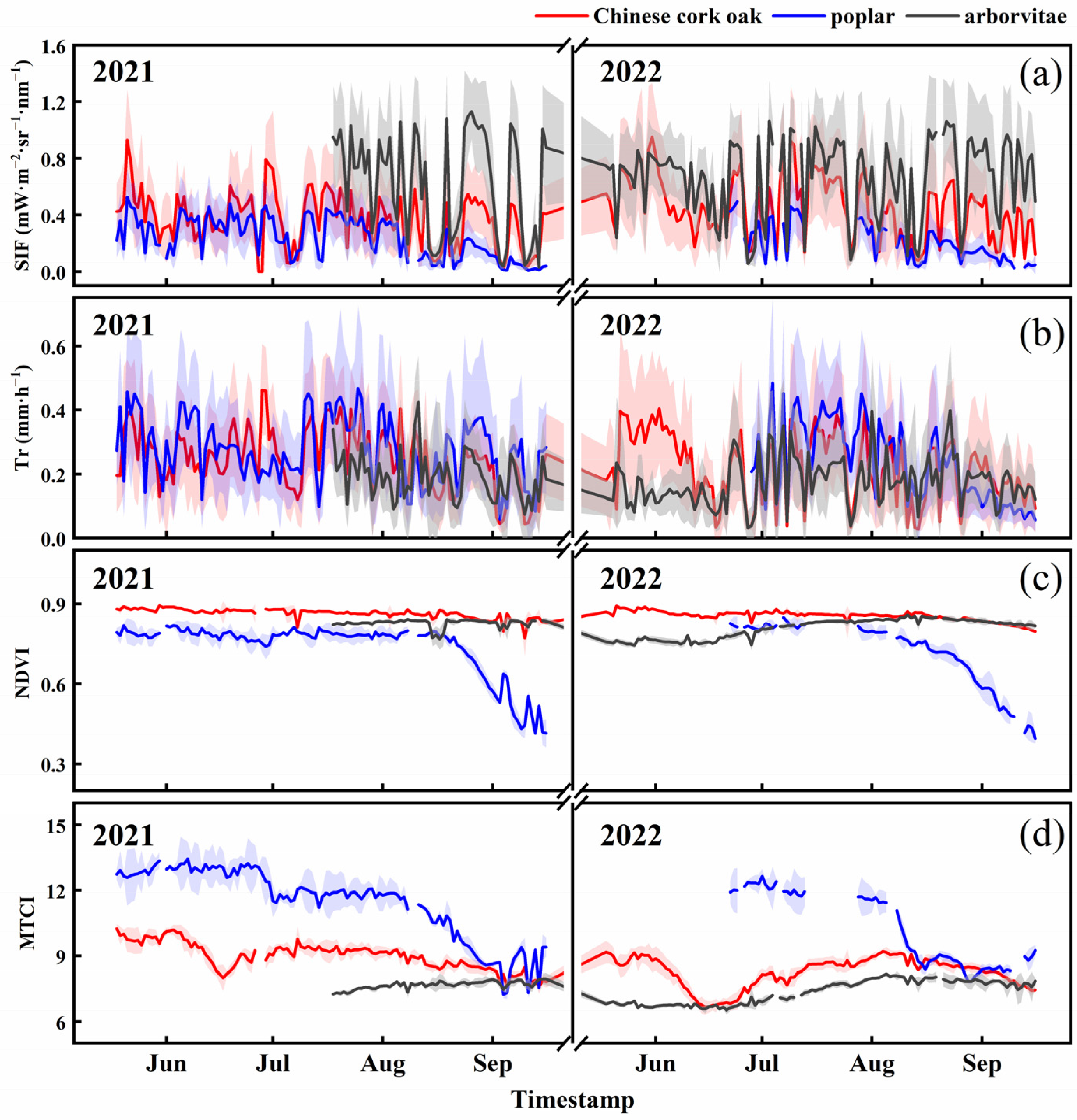
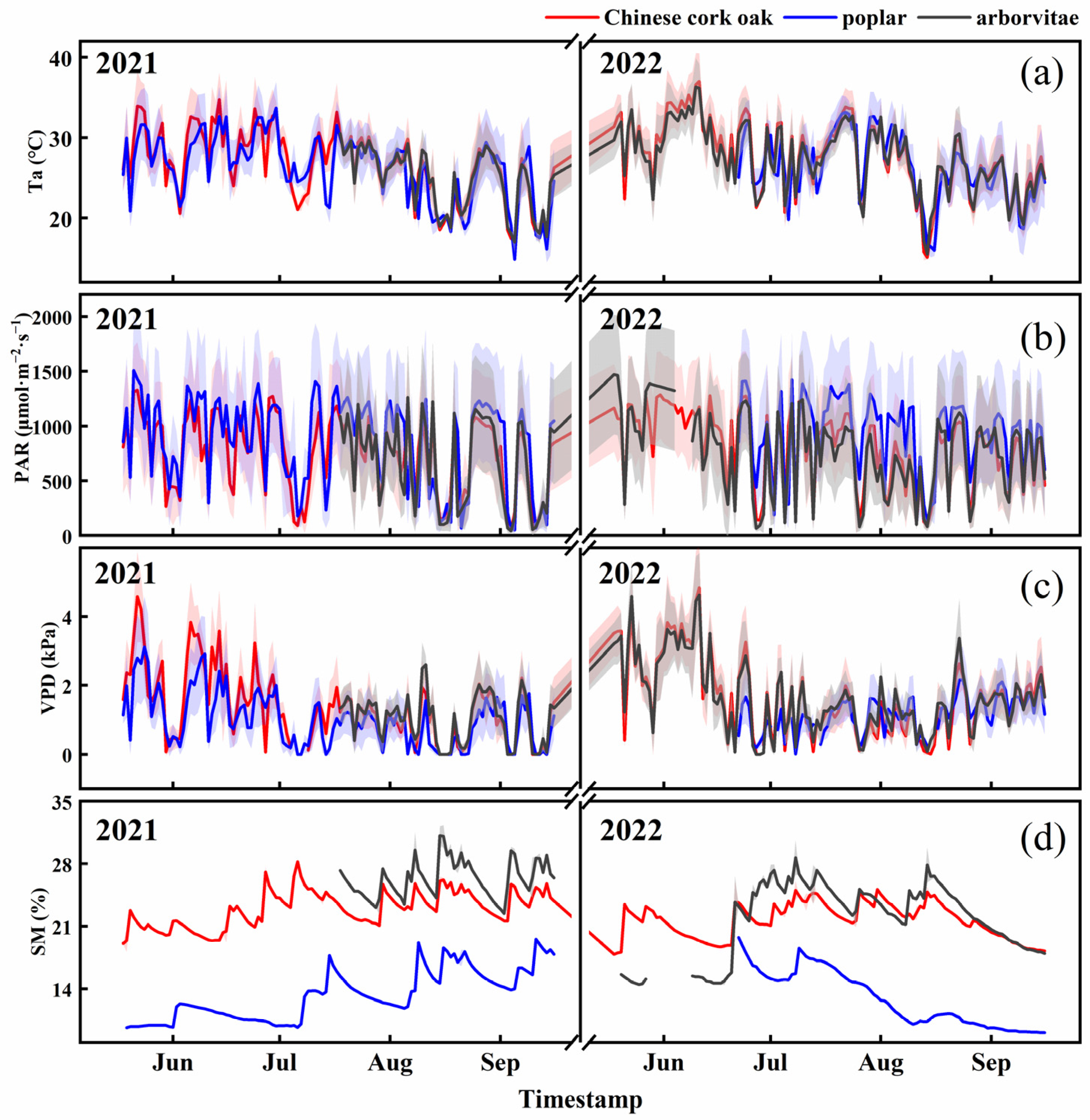
3.1. Temporal Dynamics of SIF, Tr, and Environmental Factors

From May to September in 2021–2022, daily SIF in Chinese cork oak, poplar, and arborvitae plantations exhibited day-to-day variations, with variation ranges of 0.0003–0.949 mW·m−2·sr−1·nm−1, 0.008–0.526 mW·m−2·sr−1·nm−1, and 0.031–1.133 mW·m−2·sr−1·nm−1, respectively. Overall, the daily SIF of the arborvitae plantation did not show a downward trend, while the daily SIF of the Chinese cork oak and poplar plantations began to decline in August, with the decline being more pronounced in the poplar. This could be due to differences in phenology and physiological changes among the species (Figure 1a). The NDVI of Chinese cork oak and poplar plantations remained relatively stable, whereas that of poplar plantation exhibited a marked decline during September (Figure 1c). The MTCI of Chinese cork oak and poplar plantations showed a declining trend in late August, while that of arborvitae remained stable throughout the observation period (Figure 1d). For two deciduous tree species, the earlier decline in MTCI relative to NDVI indicates that leaves might be transitioning into the senescence phase, during which chlorophyll decomposition occurs prior to the onset of the deciduous stage. Similar to the seasonal dynamics of SIF, Tr exhibited significant fluctuations. The daily Tr values in Chinese cork oak, poplar, and arborvitae plantations showed variation ranges of 0.028–0.462 mm⋅h−1, 0.056–0.486 mm⋅ mm⋅h−1, and 0.032–0.424 mm⋅h−1, respectively. The Tr in Chinese cork oak and poplar plantations began to show a declining trend in August, whereas the arborvitae plantation did not exhibit such a trend (Figure 1b).
The trends in environmental factors (including Ta, PAR, VPD, and SM) in the three plantations were relatively consistent (Figure 2). Ta began to decrease in September, with the range of variation being 15.1–37.0 °C (Chinese cork oak), 14.8–33.7 °C (poplar), and 15.5–36.3 °C (arborvitae). PAR in poplar plantation was slightly higher than that in Chinese cork oak and arborvitae plantations. VPD at all three sites reached its peak in June. The degree of air drought in Chinese cork oak and arborvitae plantations was greater than that in poplar plantation. SM was significantly affected by precipitation and showed considerable variation among the three sites, with the poplar plantation had notably lower levels compared to the Chinese cork oak and arborvitae plantations. This may be related to the differences in soil structure and water retention capacity among the sites.
In general, the SIF and Tr of the three plantations exhibited a diurnal pattern of increasing and then decreasing (Figure 3a,d,g), and the time of maximum value for SIF occurred earlier than that for Tr. After categorizing the observation days by weather conditions, distinct SIF peaks were observed for both Chinese cork oak and poplar, with Chinese cork oak peaking (12:00) earlier than poplar (12:30). The SIF of the arborvitae had no obvious peak, remaining at a relatively high level from 10:00 to 14:00. The diurnal dynamics of Tr and SIF were similar, but Tr exhibited more fluctuations and midday saturation/depression in most conditions.

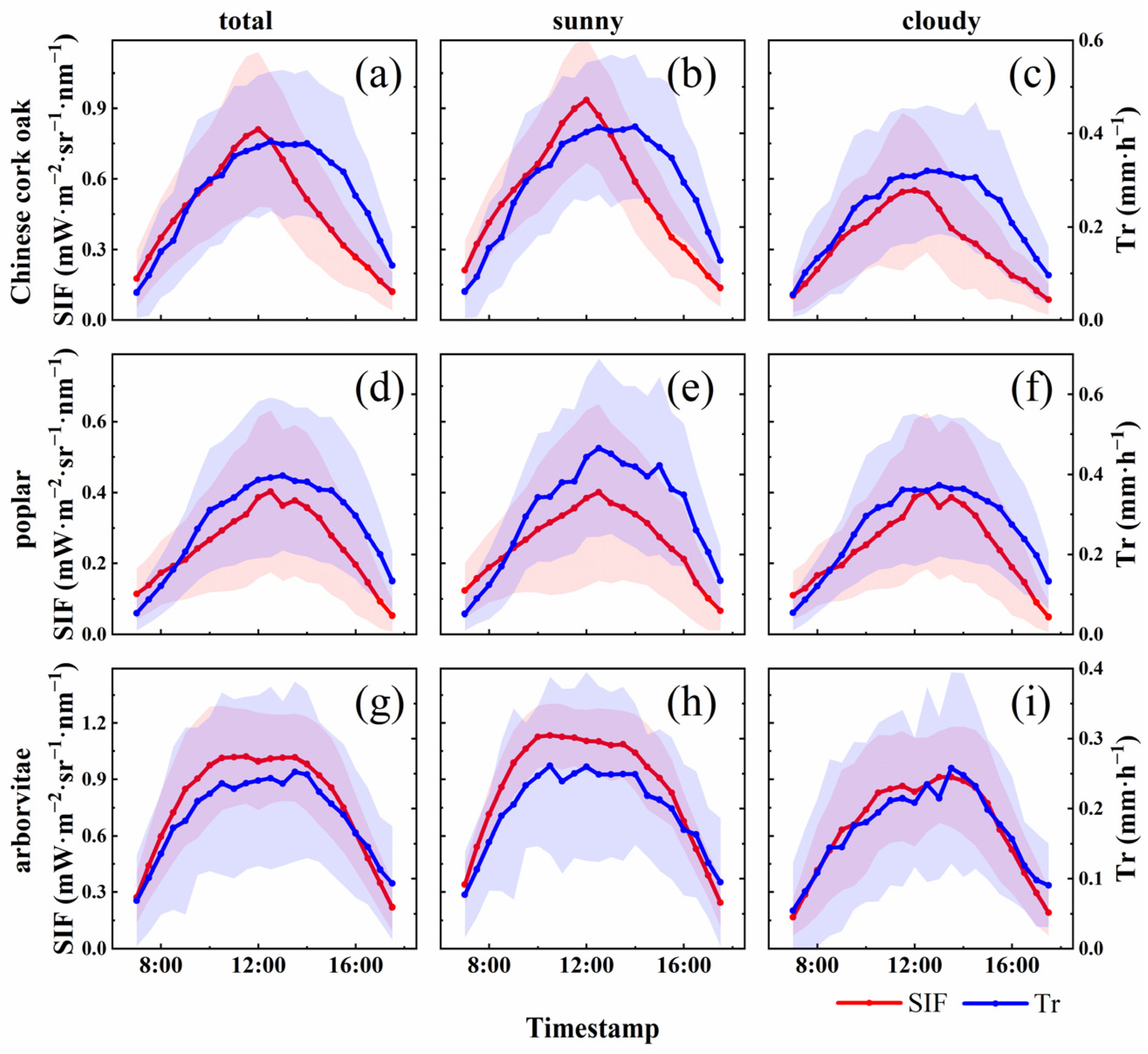
3.2. Relationships Between SIF and Tr

SIF and Tr exhibited significant linear relationships, with stronger correlation coefficients at daily scale than half-hour scale (Table 1, Figure 4). The total order of linear regression slopes (k) was poplar > Chinese cork oak > arborvitae, which suggests that poplar has a higher transpiration rate at the same level of fluorescence intensity. The differences in temporal scales did not affect k of Chinese cork oak and poplar. For arborvitae, k on the daily scale was slightly higher than on the half-hourly scale. Weather also affected the relationship between SIF and Tr. For Chinese cork oak, k, correlation coefficient, and R2 were greater on cloudy days compared to sunny days. In contrast, the relationship for poplar was stronger on sunny days. The diurnal observation time affected the correlation between SIF and Tr, altering the slope of the zero-intercept linear regression (Tr/SIF). In general, the SIF–Tr relationship exhibited a midday decrease (Figure 5). Under different weather conditions, the Tr/SIF in three plantations generally showed an increasing trend throughout the day. However, the Tr/SIF in Chinese cork oak and poplar exhibited a midday decrease on cloudy days.

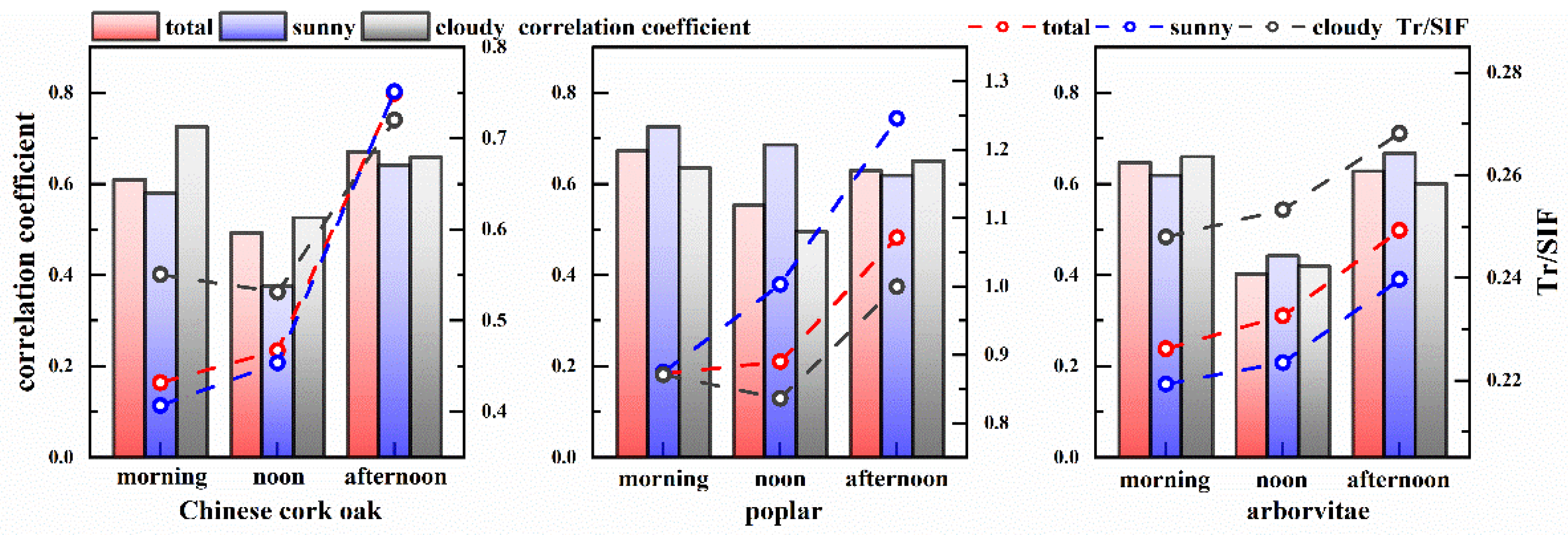
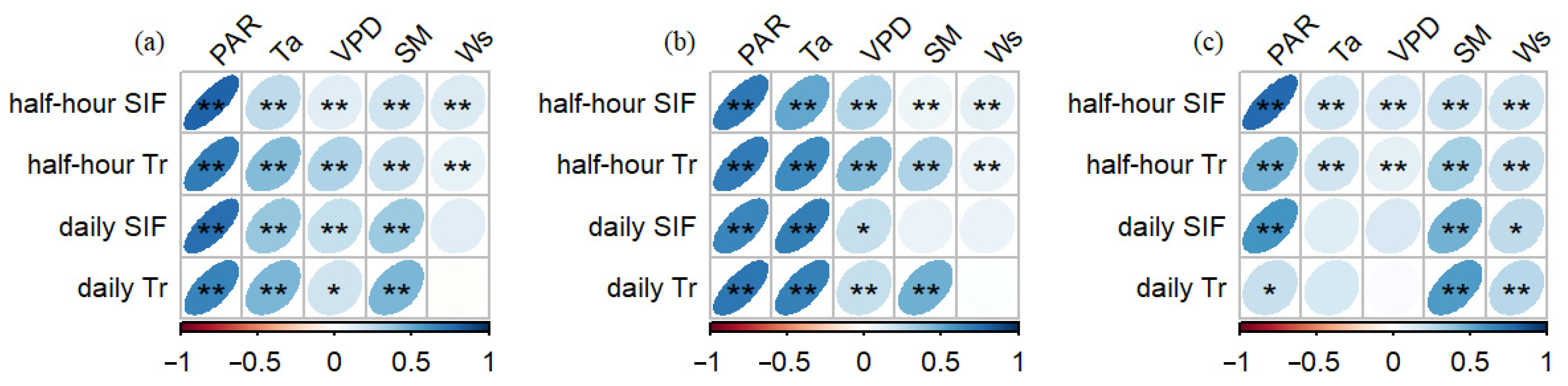
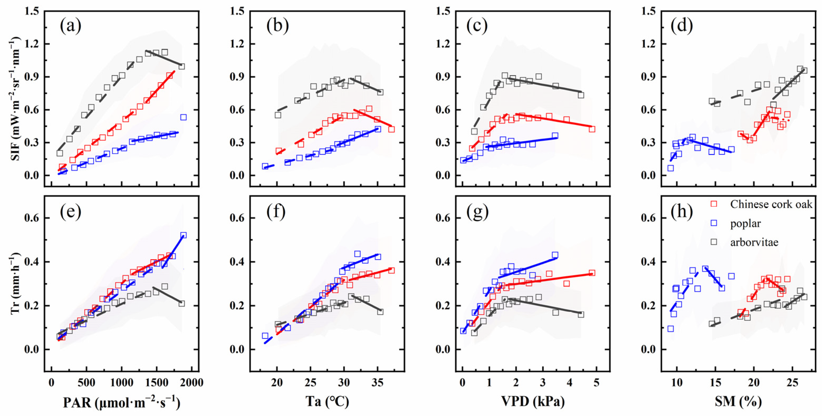
3.3. Impact of Environmental Factors on SIF, Tr, and the SIF–Tr Relationship

At the half-hour scale, SIF and Tr were more susceptible to the influence of environmental factors (Figure 6). After aggregating the temporal scale from half-hour to daily, the positive correlation between PAR and both SIF and Tr slightly weakened. In contrast, the positive correlation between Ta and both SIF and Tr strengthened for Chinese cork oak and poplar. VPD was positively correlated with both SIF and Tr, and this correlation decreased or became insignificant after temporal aggregation. Another parameter characterizing vegetation moisture availability, SM showed an enhanced positive effect on Tr and SIF after temporal aggregation.
To determine the influence of key environmental factors PAR, VPD, SM, and Ta on SIF and Tr, we aggregated the half-hour scale data based on these factors. With the increase in PAR, both SIF and Tr in Chinese cork oak and poplar showed an increasing trend (Figure 7a,e). Chinese cork oak SIF increased more rapidly at high PAR levels, while poplar SIF showed greater enhancement at low PAR. The increasing rate changes in PAR by Tr in Chinese cork oak and poplar were opposite to those of SIF. With the increase in PAR, both SIF and Tr of arborvitae initially rose and then decline, with the SIF threshold appearing slightly earlier (Figure 7a,e). The response of Chinese cork oak’s SIF and Tr to Ta showed differences; after reaching the threshold, SIF declines while Tr continued to increase, albeit at a reduced rate. As Ta increases, both SIF and Tr in poplar showed an increasing trend, but the rate of increase changes. SIF and Tr of arborvitae showed a trend of increasing first and then decreasing with the rise in Ta (Figure 7b,f). With the increase in VPD, SIF and Tr in the three plantations showed an initial rise followed by a trend of slowly increasing or decreasing, with the threshold occurring 1–2 kPa (Figure 7c,g). The impact of SM on SIF and Tr varied significantly across different plantations. For Chinese cork oak, SIF and Tr were higher when SM was at an intermediate level. Both SIF and Tr in poplar initially increased with rising SM and then decreased. As SM increases, the SIF and Tr in arborvitae rose (Figure 7d,h).
As PAR increased, the relationship between SIF and Tr (SIF–Tr) in Chinese cork oak and poplar initially showed a negative correlation, which gradually switched to a positive correlation. A decline in the SIF–Tr relationship occurred when PAR reached 1500 μmol·m−2·s−1 (Figure 8a,b). The SIF–Tr relationship in arborvitae was positively correlated at various levels of PAR, and it showed an increasing trend as PAR increased (Figure 8c). With PAR increasing, the trend of Tr/SIF was essentially opposite to that of the relationship (Figure 8a–c). As Ta raised, the SIF–Tr relationship of Chinese cork oak and poplar showed a trend of increasing initially and then decreasing, with an inflection point at approximately 26 °C (Figure 8d,e). The SIF–Tr relationship of arborvitae exhibited a decreasing trend (Figure 8f). When 1 kPa ≤ VPD < 2 kPa, the SIF–Tr relationship was relatively high, while 2 kPa ≤ VPD < 3 kPa, the SIF–Tr relationship showed a decreasing trend. As the meteorological drought intensified, the SIF−Tr relationship showed a gradual increase. When VPD > 4.5 kPa, the SIF–Tr relationship of Chinese cork oak decreased. The SIF and Tr of poplar and arborvitae exhibited similar responses to VPD, with no decline observed in the SIF–Tr relationship at high VPD (Figure 8g–i). As both Ta and VPD increased, Tr/SIF in Chinese cork oak showed an increasing trend, while for poplar and arborvitae, Tr/SIF first increased and then decreased. SM showed a higher the SIF–Tr relationship at intermediate levels, whereas excessively low or high SM levels attenuated the relationship. As SM increased, the Tr/SIF in three plantations first rose and then fell, with peak values occurring at different moisture levels (Figure 8j–l).

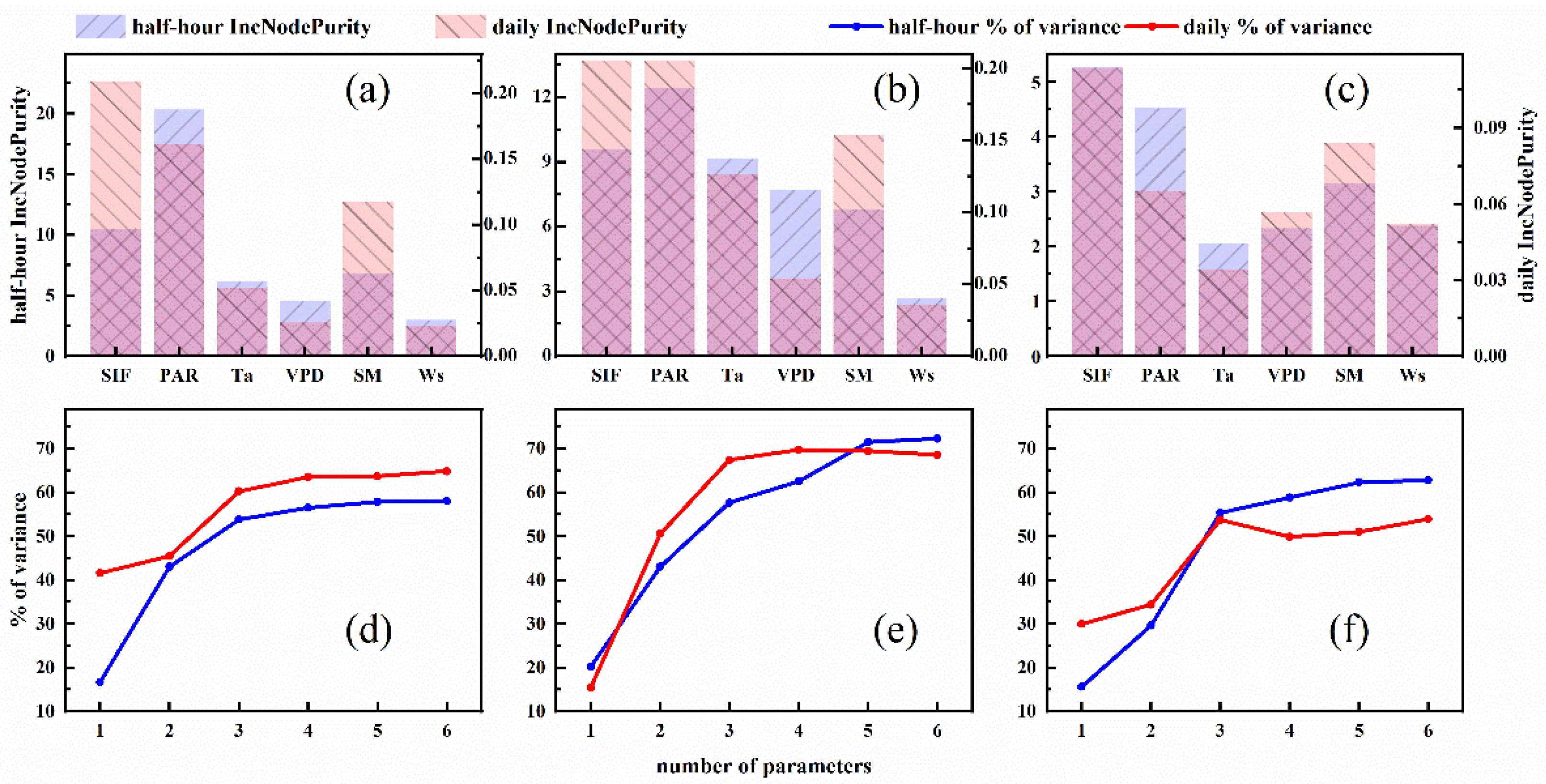
3.4. Assessing the Potential for Estimating Tr from SIF and Environmental Factors

The linear model based on the empirical relationship between SIF and Tr had R2 values of 0.33–0.39 for the half-hour scale and 0.33–0.56 for the daily scale (Table 2). The accuracy of the linear model was relatively poor, especially at the half-hour scale. We established random forest regression models using SIF and environmental factors as input variables, with Tr as the target variable. The results indicated that species and temporal scales can alter the importance ranking of factors. In all regressions, the IncNodePurity of SIF, PAR, Ta, and SM was consistently high (Figure 9a–c). With the aggregation of the temporal scale, the importance ranking of SIF and SM moved up, while the importance ranking of PAR and Ta moved down. VPD had a higher importance for poplar, while Ws had a higher importance for arborvitae. To refine the model, we sequentially eliminated the least important environmental factors based on their IncNodePurity and re-ran the regressions, continuing this process until only SIF was left. When using only SIF in the random forest regression, the variance explained ratio ranged from 15.4% to 41.55%. After incorporating all environmental factors, the variance explained ratio increased to between 53.91% and 72.27%. As the number of factors increased, the percent of variance showed an increasing trend (Figure 9d–f). Based on RMSE, R2, and the slope of zero-intercept linear regression between observations and predictions (k0), appropriately reducing less-important environmental factors will not adversely affect the model’s performance. Compared with the linear model, combining SIF with 2 to 4 important environmental factors can significantly enhance the accuracy of Tr estimation.

4. Discussion

SIF contains information about the photosynthetic physiology of vegetation, and it has the capability to estimate photosynthesis and transpiration. However, previous studies have found that the relationship between SIF and Tr has significant variability, which is influenced by environmental factors and vegetation physiology. Current research utilizing satellite data encounters significant limitations due to constraints in temporal and spatial scales, primarily focusing on the comparative analysis of vegetation functional types. To clarify the impact of environmental factors on the relationship between SIF and Tr in different plantations across various temporal scales, and to improve the reliability of SIF in estimating Tr, this study used tower-based fluorescence automatic observation systems to collect SIF data from the canopies of typical plantations such as Chinese cork oak, poplar, and arborvitae in northern China. We compared the dynamics of SIF and Tr in different plantations, examined the relationship between them, and analyzed the impact of key environmental factors on the SIF–Tr relationship.

4.1. The Temporal Dynamics of SIF and Tr in Different Species

During the canopy closure period, when the canopy structure changes slightly, the canopy SIF and Tr exhibit similar seasonal dynamic characteristics. A similar trend has been found in other forest ecosystems, which indicates that SIF can provide information about vegetation growth and condition [18]. The SIF and Tr of the two deciduous plantations showed a downward trend in September, with poplar exhibiting a stronger decline than Chinese cork oak, while no such trend was observed in the evergreen species, arborvitae. This difference is related to variations in phenology and biological rhythms among different species [44]. A series of physiological changes occur to protect the photosynthetic structures of leaves in response to declining temperatures in autumn [45]. In deciduous tree species, chlorophyll decomposition reduces light absorption, and the extensive synthesis of lutein and abscisic acid induces stomatal closure [46]. Concurrently, the stomatal control ability of aging leaves decreases, potentially leading to reduced photosynthesis and transpiration [47]. The NDVI and MTCI of arborvitae showed slight seasonal variation, consistent with the study in a subalpine conifer forest [14]. Research found that the chlorophyll content of coniferous forests remained stable throughout the year, with APAR sustaining high levels even during winter. Therefore, it mainly relied on up-regulating non-photochemical quenching (NPQ) to dissipate excessive energy and protect photosynthetic structures.
SIF and Tr are mainly driven by PAR during the day, showing an overall trend of increasing first and then decreasing, and similar trends have been observed in croplands and grasslands [32]. The diurnal dynamics of SIF and Tr exhibit differences, with SIF tending to peak around midday, while Tr saturates at midday. Chinese cork oak and arborvitae plantations exhibit midday saturation in Tr, while poplar Tr shows a distinct peak in Tr at midday on sunny days. Plants control transpiration by regulating stomatal aperture. In poplar, midday depression of Tr is absent, which may be influenced by two factors. On one hand, the VPD at the poplar’s site is relatively low, so the trees do not experience atmospheric moisture stress. On the other hand, compared to Chinese cork oak and arborvitae, poplar exhibits a more anisohydric behavior water-regulation strategy, meaning it maintains stomatal opening even under water stress to ensure carbon fixation. Cheng et al. [48] found that poplar GPP exhibits strong resistance to micrometeorological stress, which may support our view that poplar exhibits stronger anisohydric behavior. The canopy SIF of Chinese cork oak and poplar exhibits a distinct daily peak, with the rate of change being higher in the afternoon than in the morning (Figure S1). This asymmetry in daily dynamics may be attributed to the geometry of sunlight observation [49]. Differences in leaf cluster size and the average fluorescence path length can lead to variations in the intensity of SIF emitted by sunlit and shaded leaves [50]. The canopy SIF of arborvitae does not exhibit a clear midday peak, which may be related to the strong clustering of branches and foliage in coniferous species [51]. When the solar zenith angle is small, the intense reabsorption of fluorescence within the canopy reduces the ratio of fluorescence escaping from the canopy (fesc) [52], especially on sunny days (Figure S2), causing SIF to saturate as midday radiation increases [53].

4.2. The Relationship Between SIF and Tr and Their Environmental Response

In this study, SIF and Tr in three plantations both show significant correlation. Compared to traditional vegetation indices, SIF demonstrates better correlation and consistency with Tr, as SIF and Tr are linked through photosynthetic physiology and stomatal behavior [18]. Therefore, the covariation relationship between fluorescence emission and photochemistry (light energy distribution), as well as the degree of coupling between photosynthesis and transpiration (stomatal control), will affect the relationship between SIF and Tr. Consistent with previous research, the correlation between SIF and Tr strengthens as the temporal scale is aggregated [18]. Temporal aggregation reduces response differences between SIF and Tr to environmental variations at the half-hour scale, along with mitigating random observation noise effects, thereby enhancing their correlation. Furthermore, the scale-dependent relationship between SIF and Tr is largely attributable to their co-variation with environmental factors. Temporal aggregation reduces the range of variation in SIF, Tr, and environmental factors. Notably, SIF and photosynthesis exhibit a strong linear relationship under moderate radiation levels, while photosynthesis and transpiration are strongly linked under favorable environmental conditions. These mechanisms collectively enhance the indirect linkage between SIF and Tr.
At midday, short-term stressors diminish the correlation. Research on SIF and GPP within forest ecosystems has revealed that GPP reaches saturation at midday, a phenomenon not observed with SIF. This disparity is the primary driver of their nonlinear correlation [48]. SIF is related to the photoreaction phase of photosynthesis and is independent of the dark reaction phase. The main reasons for GPP saturation are twofold: firstly, due to the limitation of the photosynthetic substrates in the chloroplasts, the rate of the dark reaction becomes saturated when the input of photosynthetically active radiation reaches a threshold value; secondly, under the stress of water, heat, and radiation, vegetation adopts measures to mitigate the harm of short-term stress, including closing stomata to protect hydraulic integrity, regulating the efficiency of PSII in absorbing light, and upregulating NPQ to prevent photochemical damage to the leaves [54,55]. Stomatal closure will decouple the processes of photosynthesis and transpiration, and the relationship between SIF and Tr will be diminished. The gradual increase in Tr/SIF may be related to the diurnal dynamic changes in SIF and Tr. In the afternoon, the slope of Tr is less steep than that in the morning, while the trend for SIF shows the opposite pattern (Figure S1). The time of satellite observation of SIF at a specific location is fixed. Differences in diurnal observation time can affect the relationship and slope between SIF and Tr. Therefore, temporal effects should be considered when using satellite SIF.
During the period of canopy stability, environmental factors predominantly influence changes in SIF and Tr. Correlation analysis showed that SIF and Tr were more sensitive to environmental factors at the half-hour scale. Therefore, high temporal resolution observation data are better suited for analyzing vegetation responses to environmental factors. Covariance between factors may obscure their actual effects, but partial correlation analysis indicates that SIF and Tr consistently show a correlation (Figure S3). SIF is the light emitted after photon transitions, during which the light-harvesting antenna absorbs light and transfers the energy to PSII. Driven by incoming radiation, Fs shows a strong correlation with PAR [56]. Stomata are the main channels for plant transpiration. Stomatal response to radiation involves both circadian rhythms and guard cell photoreceptors that activate proton pumps under blue light, driving ion uptake and osmotic changes to open stomata [57]. Therefore, radiation also drives Tr. The rate of CO2 diffusion from the environment to the chloroplasts increases with rising temperatures. Photosynthesis involves a series of enzymatic reactions, and the activity of the Rubisco is crucial in the process of CO2 fixation. Ta can affect the rate of enzymatic reactions [58]. When the temperature increases, the vapor pressure inside the leaf rises more than the vapor pressure of the surrounding air. This difference in vapor pressure between the inside and outside of the leaf enhances the transpiration rate. VPD creates a greater evaporative demand, but an increase in VPD also leads to leaf water loss, which in turn induces stomatal closure. After accounting for the covariation with PAR or Ta, VPD generally has a negative effect on SIF and Tr (Figure S4). When soil moisture is sufficient, plants can fully utilize water for transpiration to regulate leaf temperature and facilitate nutrient transport. SM and VPD collectively influence stomatal conductance and transpiration rate [59]. The increase in Ws can reduce the thickness of the vapor boundary layer around the leaves, thereby decreasing diffusion resistance and increasing the transpiration rate. At the same time, a light Ws can carry away vapor, increasing evaporative demand. However, strong winds can cause guard cells to lose water rapidly, leading to stomatal closure.
After analyzing the actual observation results, it was found that when key environmental factors reached a threshold, the trends of SIF and Tr changed [21]. To prevent hydraulic failure, plants employ a range of mechanisms, including both structural and physiological adjustments [60]. When environmental conditions exceed the optimal range for vegetation, the elevated transpiration rate leads to leaf water loss. To balance water potential, plants may close stomata or increase the uptake of soil moisture. In the short term, stomatal closure is the primary mechanism plants use to limit transpiration loss. At noon, under high levels of PAR, Ta, and VPD, vegetation undergoes short-term stress, leading to a decline in both SIF and Tr. The fraction of open PSII reaction centers (qL) gradually decreases with increasing PAR, qL decreases, and the rate of photon absorption declines [61]. During thermal stress, leaves trade off the potential thermal dissipation demand with the need for water saving due to increased evaporation [62]. When water loss exceeds the threshold, the photosystem enhances photorespiration to protect photosynthetic structures. Stomatal responses to environmental factors are related to water availability and are influenced by the water supply and demand balance [63]. SM and VPD collectively determine stomatal conductance by affecting leaf water potential, with plants in dry locations having stomata that are more sensitive to changes in VPD [64].
Due to differences in hydraulic architecture, plants regulate transpiration differently to maintain water balance. Isohydric plants exhibit stricter stomatal control, while anisohydric species have weaker regulation of Tr [65]. The minimum water potential for survival is determined by the vulnerability of the hydraulic structure, and differences in structure account for the variation in water potential regulation among species [66]. Species with lower xylem embolism resistance tend to have more sensitive stomatal control [67]. In diffuse-porous species, the vessel diameters are small and densely distributed in the sapwood, contributing to greater hydraulic. In ring-porous species, the vessel diameters are large and only distributed in the sapwood of recent years, which increases the risk of embolism. Therefore, the Chinese cork oak (ring-porous) experiences a decline in Tr during midday, while poplar (diffuse-porous) exhibits a peak in Tr at noon on sunny days. The response of GPP to PAR confirms that the stomata of Chinese cork oak are more sensitive to stress than poplar [48]. Compared to the two deciduous species, the water transport in non-porous wood is carried out through tracheid, and the threshold of environmental response for the SIF and Tr of arborvitae is lower. Non-porous species have not formed continuous tubular structures, and tracheids have smaller diameters and are enclosed by cell walls, which results in a slower water transport rate and a lower risk of embolism. Arborvitae typically utilizes leaf desiccation and lower water potential to regulate stomatal response during drought conditions [68]. Xylem resistance to embolism is positively correlated with root depth [69]. Chinese cork oak and arborvitae are located in mountainous areas with thin soil layers, making it difficult for the roots to access groundwater. In contrast, the poplar site is situated in a plain where groundwater resources are abundant and easily accessible to the roots. Therefore, Chinese cork oak and arborvitae respond to drought through sensitive stomatal control.

4.3. Evaluation of Estimating Tr from SIF and Environmental Factors

The results of the random forest importance analysis indicate that there are differences in the environmental factors affecting Tr at different temporal scales. Overall, an increase in temporal scale tends to diminish the contribution of PAR and VPD to Tr, while enhancing the contribution of Ta and SM to Tr, which is consistent with the results of the correlation analysis. The long-term changes in vegetation Tr are usually determined by Ta and SM, which control or influence biological rhythms and hydraulic properties [70]. During the day, radiation is the switch that induces stomatal opening for water and carbon exchange [71], making micrometeorological factors the main regulatory variables for stomatal conductance. Ws primarily affects SIF by altering canopy structure through leaf rolling and displacement [72], and influences Tr by changing leaf temperature and vapor movement. The significant contribution of Ws to arborvitae Tr may be due to the location on the southern hillside, where Ws is higher. The complexity of the influence of environmental factors on SIF, Tr, and the SIF–Tr relationship makes it impossible to ensure the accuracy of a single linear model [73]. Incorporating environmental factors into the model can enhance the ability of SIF to simulate Tr to varying extents.
Based on SIF, appropriately incorporating environmental factors into the model leads to a reduction in RMSE, an increase in R2, and k0 will more closely approach 1. The number of variables and the selection of variables can affect the accuracy of the simulation. When choosing environmental factors, the impact of tree species and temporal scales should be considered. The results of the model may be species-specific. Deciduous species may require more factors than evergreen species, and higher resolution temporal scales may require more factors. The model performance ranking across the three plantations is as follows: poplar > Chinese cork oak > arborvitae, and Maes et al. [16] also found that the correlation between SIF and Tr in deciduous forests is higher than in evergreen broad-leaved forests. Overestimation at low SIF and underestimation at high SIF may be the main reasons for the smaller k0. This study assumes ET to be Tr during the full leaf period; however, in reality, soil evaporation is not zero. This study is based on the analysis of a period with relatively stable canopy structure and excludes the effects of canopy structure changes. In fact, canopy structural characteristics such as LAI, leaf inclination angle, and clumping index can affect the direct and diffuse radiation received by leaves within the canopy, as well as the scattering and reabsorption processes of emitted fluorescence within the canopy. Therefore, when studying canopies with drastic structural changes, the influence of canopy parameters must be taken into account. This study mainly considered the impact of environmental factors; however, throughout the growing season, growth stage, canopy structure, and other physiological factors also affect the ability of SIF to estimate Tr. In future research, to improve the reliability of SIF in estimating Tr, the impact of soil evaporation and plant physiology should be taken into account.

5. Conclusions

This study simultaneously monitored SIF and Tr in three plantations in northern China, focusing on analyzing the species-specific responses of the SIF–Tr relationship to environmental changes and using SIF along with environmental factors to model Tr. The study found significant differences in the dynamic patterns of SIF and Tr among different tree species. As the season progressed, the deciduous species showed a decline in SIF and Tr in September due to leaf senescence, while the evergreen species did not exhibit the same trend. With the aggregation of temporal scales, the correlation between SIF and Tr strengthened. There is a threshold in the influence of environmental factors on SIF and Tr, which affects the SIF–Tr relationship. Incorporating environmental factors into the SIF model significantly improves the accuracy of Tr simulation. The extent of accuracy improvement and the selection of environmental factors are influenced by temporal scales and tree species. The influence of the environment on SIF, Tr, and the SIF–Tr relationship shows significant species specificity. Currently, the vegetation functional classification used in remote sensing may obscure the SIF–Tr relationship among different tree species. Therefore, future research should supplement observational datasets from various tree species and build a comprehensive understanding of how environmental factors influence SIF and Tr, to achieve reliable applications at the remote sensing scale.

Supplementary Materials

The following supporting information can be downloaded at: https://www.mdpi.com/article/10.3390/rs17091625/s1, Text S1: Calculation of fluorescence escape ratio (fesc); Text S2: Partial correlation analysis; Figure S1: The impact of PAR on SIF (left) and Tr (right) in Chinese cork oak (hollow triangle), poplar (hollow square), and arborvitae (solid square) plantations; Figure S2: Diurnal dynamics of the fluorescence escape ratio (fesc) in Chinese cork oak (a), poplar (b), and arborvitae (c) plantations under different weather conditions; Figure S3: The partial correlation coefficient of SIF and Tr with different environmental factors as controlled variables in plantations at half-hour (a) and daily (b) scales; Figure S4: The partial correlation coefficients of VPD with SIF and Tr after controlling for PAR (a) and Ta (b) in plantations at half-hour and daily scales.

Author Contributions

Conceptualization, J.Z. and S.S.; methodology, M.H. and X.C.; software, M.H. and X.W.; validation, Q.P. and C.G.; data curation, X.G. and Z.L.; writing—original draft preparation, M.H.; writing—review and editing, J.Z.; visualization, M.H.; supervision, J.Z. and S.S.; funding acquisition, S.S. All authors have read and agreed to the published version of the manuscript.

Funding

This study was funded by grant number CAFYBB2023PA001.

Data Availability Statement

The datasets generated during and/or analyzed during the current study are available from the corresponding author on reasonable request.

Acknowledgments

We thank Guang Lu from Nanshan Forest Farm for the in situ observations. We are grateful to Yongbin Huang, Min Wang, and Chaoyue Wu for assistance with instrument maintenance.

Conflicts of Interest

The authors declare no conflicts of interest.

References

  1. Monteith, J.L. Evaporation and environment. In Proceedings of the Symposia of the Society for Experimental Biology; Cambridge University Press: Cambridge, UK, 1965; pp. 205–234. [Google Scholar]
  2. Schlesinger, W.H.; Jasechko, S. Transpiration in the global water cycle. Agric. For. Meteorol. 2014, 189–190, 115–117. [Google Scholar] [CrossRef]
  3. Fisher, J.B.; Melton, F.; Middleton, E.; Hain, C.; Anderson, M.; Allen, R.; McCabe, M.F.; Hook, S.; Baldocchi, D.; Townsend, P.A. The future of evapotranspiration: Global requirements for ecosystem functioning, carbon and climate feedbacks, agricultural management, and water resources. Water Resour. Res. 2017, 53, 2618–2626. [Google Scholar] [CrossRef]
  4. Li, X.; Gentine, P.; Lin, C.; Zhou, S.; Sun, Z.; Zheng, Y.; Liu, J.; Zheng, C. A simple and objective method to partition evapotranspiration into transpiration and evaporation at eddy-covariance sites. Agric. For. Meteorol. 2019, 265, 171–182. [Google Scholar] [CrossRef]
  5. Talsma, C.J.; Good, S.P.; Jimenez, C.; Martens, B.; Fisher, J.B.; Miralles, D.G.; McCabe, M.F.; Purdy, A.J. Partitioning of evapotranspiration in remote sensing-based models. Agric. For. Meteorol. 2018, 260, 131–143. [Google Scholar] [CrossRef]
  6. Sun, X.; Wilcox, B.P.; Zou, C.B. Evapotranspiration partitioning in dryland ecosystems: A global meta-analysis of in situ studies. J. Hydrol. 2019, 576, 123–136. [Google Scholar] [CrossRef]
  7. Senay, G.B.; Bohms, S.; Singh, R.K.; Gowda, P.H.; Velpuri, N.M.; Alemu, H.; Verdin, J.P. Operational Evapotranspiration Mapping Using Remote Sensing and Weather Datasets: A New Parameterization for the SSEB Approach. J. Am. Water Resour. Assoc. 2013, 49, 577–591. [Google Scholar] [CrossRef]
  8. Zeng, Z.; Wang, T.; Zhou, F.; Ciais, P.; Mao, J.; Shi, X.; Piao, S. A worldwide analysis of spatiotemporal changes in water balance-based evapotranspiration from 1982 to 2009. J. Geophys. Res. Atmos. 2014, 119, 1186–1202. [Google Scholar] [CrossRef]
  9. Mu, Q.; Zhao, M.; Running, S.W. Improvements to a MODIS global terrestrial evapotranspiration algorithm. Remote Sens. Environ. 2011, 115, 1781–1800. [Google Scholar] [CrossRef]
  10. Jung, M.; Reichstein, M.; Ciais, P.; Seneviratne, S.I.; Sheffield, J.; Goulden, M.L.; Bonan, G.; Cescatti, A.; Chen, J.; De Jeu, R. Recent decline in the global land evapotranspiration trend due to limited moisture supply. Nature 2010, 467, 951–954. [Google Scholar] [CrossRef]
  11. Porcar-Castell, A.; Tyystjärvi, E.; Atherton, J.; Van der Tol, C.; Flexas, J.; Pfündel, E.E.; Moreno, J.; Frankenberg, C.; Berry, J.A. Linking chlorophyll a fluorescence to photosynthesis for remote sensing applications: Mechanisms and challenges. J. Exp. Bot. 2014, 65, 4065–4095. [Google Scholar] [CrossRef]
  12. Badgley, G.; Field, C.B.; Berry, J.A. Canopy near-infrared reflectance and terrestrial photosynthesis. Sci. Adv. 2017, 3, e1602244. [Google Scholar] [CrossRef] [PubMed]
  13. Rossini, M.; Nedbal, L.; Guanter, L.; Ač, A.; Alonso, L.; Burkart, A.; Cogliati, S.; Colombo, R.; Damm, A.; Drusch, M. Red and far red Sun-induced chlorophyll fluorescence as a measure of plant photosynthesis. Geophys. Res. Lett. 2015, 42, 1632–1639. [Google Scholar] [CrossRef]
  14. Magney, T.S.; Bowling, D.R.; Logan, B.A.; Grossmann, K.; Stutz, J.; Blanken, P.D.; Burns, S.P.; Cheng, R.; Garcia, M.A.; Köhler, P. Mechanistic evidence for tracking the seasonality of photosynthesis with solar-induced fluorescence. Proc. Natl. Acad. Sci. USA 2019, 116, 11640–11645. [Google Scholar] [CrossRef] [PubMed]
  15. Zhang, Y.; Guanter, L.; Berry, J.A.; Joiner, J.; van der Tol, C.; Huete, A.; Gitelson, A.; Voigt, M.; Köhler, P. Estimation of vegetation photosynthetic capacity from space-based measurements of chlorophyll fluorescence for terrestrial biosphere models. Glob. Change Biol. 2014, 20, 3727–3742. [Google Scholar] [CrossRef]
  16. Maes, W.H.; Pagán, B.R.; Martens, B.; Gentine, P.; Guanter, L.; Steppe, K.; Verhoest, N.E.; Dorigo, W.; Li, X.; Xiao, J. Sun-induced fluorescence closely linked to ecosystem transpiration as evidenced by satellite data and radiative transfer models. Remote Sens. Environ. 2020, 249, 112030. [Google Scholar] [CrossRef]
  17. Zhou, K.; Zhang, Q.; Xiong, L.; Gentine, P. Estimating evapotranspiration using remotely sensed solar-induced fluorescence measurements. Agric. For. Meteorol. 2022, 314, 108800. [Google Scholar] [CrossRef]
  18. Lu, X.; Liu, Z.; An, S.; Miralles, D.G.; Maes, W.; Liu, Y.; Tang, J. Potential of solar-induced chlorophyll fluorescence to estimate transpiration in a temperate forest. Agric. For. Meteorol. 2018, 252, 75–87. [Google Scholar] [CrossRef]
  19. Alemohammad, S.H.; Fang, B.; Konings, A.G.; Aires, F.; Green, J.K.; Kolassa, J.; Miralles, D.; Prigent, C.; Gentine, P. Water, Energy, and Carbon with Artificial Neural Networks (WECANN): A statistically based estimate of global surface turbulent fluxes and gross primary productivity using solar-induced fluorescence. Biogeosciences 2017, 14, 4101–4124. [Google Scholar] [CrossRef]
  20. Beauclaire, Q.; De Cannière, S.; Jonard, F.; Pezzetti, N.; Delhez, L.; Longdoz, B. Modeling gross primary production and transpiration from sun-induced chlorophyll fluorescence using a mechanistic light-response approach. Remote Sens. Environ. 2024, 307, 114150. [Google Scholar] [CrossRef]
  21. Damm, A.; Haghighi, E.; Paul-Limoges, E.; van der Tol, C. On the seasonal relation of sun-induced chlorophyll fluorescence and transpiration in a temperate mixed forest. Agric. For. Meteorol. 2021, 304, 108386. [Google Scholar] [CrossRef]
  22. Pagán, B.R.; Maes, W.H.; Gentine, P.; Martens, B.; Miralles, D.G. Exploring the potential of satellite solar-induced fluorescence to constrain global transpiration estimates. Remote Sens. 2019, 11, 413. [Google Scholar] [CrossRef]
  23. Song, L.; Ding, Z.; Kustas, W.P.; Hua, W.; Liu, X.; Liu, L.; Liu, S.; Ma, M.; Bai, Y.; Xu, Z. Applications of a Thermal-Based Two-Source Energy Balance Model Coupling the Sun-Induced Chlorophyll Fluorescence Data. IEEE Geosci. Remote Sens. Lett. 2023, 20, 1–5. [Google Scholar] [CrossRef]
  24. Yang, J.; Liu, Z.; Yu, Q.; Lu, X. Estimation of global transpiration from remotely sensed solar-induced chlorophyll fluorescence. Remote Sens. Environ. 2024, 303, 113998. [Google Scholar] [CrossRef]
  25. Liu, Y.; Zhang, Y.; Shan, N.; Zhang, Z.; Wei, Z. Global assessment of partitioning transpiration from evapotranspiration based on satellite solar-induced chlorophyll fluorescence data. J. Hydrol. 2022, 612, 128044. [Google Scholar] [CrossRef]
  26. Shan, N.; Zhang, Y.; Chen, J.M.; Ju, W.; Goulas, Y. A model for estimating transpiration from remotely sensed solar-induced chlorophyll fluorescence. Remote Sens. Environ. 2021, 252, 112134. [Google Scholar] [CrossRef]
  27. Zhang, Q.; Liu, X.; Zhou, K.; Zhou, Y.; Gentine, P.; Pan, M.; Katul, G.G. Solar-induced chlorophyll fluorescence sheds light on global evapotranspiration. Remote Sens. Environ. 2024, 305, 114061. [Google Scholar] [CrossRef]
  28. Shang, K.; Yao, Y.; Di, Z.; Jia, K.; Zhang, X.; Fisher, J.B.; Chen, J.; Guo, X.; Yang, J.; Yu, R. Coupling physical constraints with machine learning for satellite-derived evapotranspiration of the Tibetan Plateau. Remote Sens. Environ. 2023, 289, 113519. [Google Scholar] [CrossRef]
  29. Zheng, C.; Wang, S.; Chen, J.M.; Xiao, J.; Chen, J.; Zhu, K.; Sun, L. Modeling transpiration using solar-induced chlorophyll fluorescence and photochemical reflectance index synergistically in a closed-canopy winter wheat ecosystem. Remote Sens. Environ. 2024, 302, 113981. [Google Scholar] [CrossRef]
  30. Kira, O.; Sun, Y. Extraction of sub-pixel C3/C4 emissions of solar-induced chlorophyll fluorescence (SIF) using artificial neural network. ISPRS J. Photogramm. Remote Sens. 2020, 161, 135–146. [Google Scholar] [CrossRef]
  31. Gu, L.; Wood, J.D.; Chang, C.Y.; Sun, Y.; Riggs, J.S. Advancing terrestrial ecosystem science with a novel automated measurement system for sun-induced chlorophyll fluorescence for integration with eddy covariance flux networks. J. Geophys. Res. Biogeosci. 2019, 124, 127–146. [Google Scholar] [CrossRef]
  32. Shan, N.; Ju, W.; Migliavacca, M.; Martini, D.; Guanter, L.; Chen, J.; Goulas, Y.; Zhang, Y. Modeling canopy conductance and transpiration from solar-induced chlorophyll fluorescence. Agric. For. Meteorol. 2019, 268. [Google Scholar] [CrossRef]
  33. Martínez-Vilalta, J.; Garcia-Forner, N. Water potential regulation, stomatal behaviour and hydraulic transport under drought: Deconstructing the iso/anisohydric concept. Plant Cell Environ. 2017, 40, 962–976. [Google Scholar] [CrossRef]
  34. Liu, X.; Liu, L.; Hu, J.; Guo, J.; Du, S. Improving the potential of red SIF for estimating GPP by downscaling from the canopy level to the photosystem level. Agric. For. Meteorol. 2020, 281, 107846. [Google Scholar] [CrossRef]
  35. Mazzoni, M.; Falorni, P.; Del Bianco, S. Sun-induced leaf fluorescence retrieval in the O2-B atmospheric absorption band. Opt. Express 2008, 16, 7014–7022. [Google Scholar] [CrossRef]
  36. Hu, M.; Cheng, X.; Zhang, J.; Huang, H.; Zhou, Y.; Wang, X.; Pan, Q.; Guan, C. Temporal Variation in Tower-Based Solar-Induced Chlorophyll Fluorescence and Its Environmental Response in a Chinese Cork Oak Plantation. Remote Sens. 2023, 15, 3568. [Google Scholar] [CrossRef]
  37. Allen, R.G.; Pereira, L.S.; Raes, D.; Smith, M. Crop Evapotranspiration—Guidelines for Computing Crop Water Requirements—FAO Irrigation and Drainage Paper 56; FAO: Rome, Italy, 1998; Volume 300, p. D05109. [Google Scholar]
  38. Rouse, J.W.; Haas, R.H.; Schell, J.A.; Deering, D.W. Monitoring vegetation systems in the Great Plains with ERTS. NASA Spec. Publ. 1974, 351, 309. [Google Scholar]
  39. Viña, A.; Gitelson, A.A.; Nguy-Robertson, A.L.; Peng, Y. Comparison of different vegetation indices for the remote assessment of green leaf area index of crops. Remote Sens. Environ. 2011, 115, 3468–3478. [Google Scholar] [CrossRef]
  40. Gu, L.; Fuentes, J.D.; Shugart, H.H.; Staebler, R.M.; Black, T.A. Responses of net ecosystem exchanges of carbon dioxide to changes in cloudiness: Results from two North American deciduous forests. J. Geophys. Res. Atmos. 1999, 104, 31421–31434. [Google Scholar] [CrossRef]
  41. Li, Z.; Zhang, Q.; Li, J.; Yang, X.; Wu, Y.; Zhang, Z.; Wang, S.; Wang, H.; Zhang, Y. Solar-induced chlorophyll fluorescence and its link to canopy photosynthesis in maize from continuous ground measurements. Remote Sens. Environ. 2020, 236, 111420. [Google Scholar] [CrossRef]
  42. Kumar, R.; Umanand, L. Estimation of global radiation using clearness index model for sizing photovoltaic system. Renew. Energy 2005, 30, 2221–2233. [Google Scholar] [CrossRef]
  43. Belgiu, M.; Drăguţ, L. Random forest in remote sensing: A review of applications and future directions. ISPRS J. Photogramm. Remote Sens. 2016, 114, 24–31. [Google Scholar] [CrossRef]
  44. Wang, F.; Chen, B.; Lin, X.; Zhang, H. Solar-induced chlorophyll fluorescence as an indicator for determining the end date of the vegetation growing season. Ecol. Indic. 2020, 109, 105755. [Google Scholar] [CrossRef]
  45. Biswal, B.; Krupinska, K.; Biswal, U.C. Plastid Development in Leaves During Growth and Senescence; Springer: Dordrecht, The Netherlands, 2013; Volume 36. [Google Scholar]
  46. Chaves, M.M.; Flexas, J.; Pinheiro, C. Photosynthesis under drought and salt stress: Regulation mechanisms from whole plant to cell. Ann. Bot. 2009, 103, 551–560. [Google Scholar] [CrossRef] [PubMed]
  47. Wardle, K.; Short, K. Stomatal response of in vitro cultured plantlets. I. Responses in epidermal strips of Chrysanthemum to environmental factors and growth regulators. Biochem. Physiol. Pflanzen 1983, 178, 619–624. [Google Scholar] [CrossRef]
  48. Cheng, X.; Hu, M.; Zhou, Y.; Wang, F.; Liu, L.; Wang, Y.; Huang, H.; Zhang, J. The divergence of micrometeorology sensitivity leads to changes in GPP/SIF between cork oak and poplar. Agric. For. Meteorol. 2022, 326, 109189. [Google Scholar] [CrossRef]
  49. Yang, X.; Tang, J.; Mustard, J.F.; Lee, J.E.; Rossini, M.; Joiner, J.; Munger, J.W.; Kornfeld, A.; Richardson, A.D. Solar-induced chlorophyll fluorescence that correlates with canopy photosynthesis on diurnal and seasonal scales in a temperate deciduous forest. Geophys. Res. Lett. 2015, 42, 2977–2987. [Google Scholar] [CrossRef]
  50. Damm, A.; Guanter, L.; Paul-Limoges, E.; Van der Tol, C.; Hueni, A.; Buchmann, N.; Eugster, W.; Ammann, C.; Schaepman, M.E. Far-red sun-induced chlorophyll fluorescence shows ecosystem-specific relationships to gross primary production: An assessment based on observational and modeling approaches. Remote Sens. Environ. 2015, 166, 91–105. [Google Scholar] [CrossRef]
  51. Louis, J.; Ounis, A.; Ducruet, J.-M.; Evain, S.; Laurila, T.; Thum, T.; Aurela, M.; Wingsle, G.; Alonso, L.; Pedros, R. Remote sensing of sunlight-induced chlorophyll fluorescence and reflectance of Scots pine in the boreal forest during spring recovery. Remote Sens. Environ. 2005, 96, 37–48. [Google Scholar] [CrossRef]
  52. Zeng, Y.; Badgley, G.; Dechant, B.; Ryu, Y.; Chen, M.; Berry, J.A. A practical approach for estimating the escape ratio of near-infrared solar-induced chlorophyll fluorescence. Remote Sens. Environ. 2019, 232, 111209. [Google Scholar] [CrossRef]
  53. Rochdi, N.; Fernandes, R.; Chelle, M. An assessment of needles clumping within shoots when modeling radiative transfer within homogeneous canopies. Remote Sens. Environ. 2006, 102, 116–134. [Google Scholar] [CrossRef]
  54. Paul-Limoges, E.; Damm, A.; Hueni, A.; Liebisch, F.; Eugster, W.; Schaepman, M.E.; Buchmann, N. Effect of environmental conditions on sun-induced fluorescence in a mixed forest and a cropland. Remote Sens. Environ. 2018, 219, 310–323. [Google Scholar] [CrossRef]
  55. Zhang, Y.; Xiao, X.; Wolf, S.; Wu, J.; Wu, X.; Gioli, B.; Wohlfahrt, G.; Cescatti, A.; Van der Tol, C.; Zhou, S. Spatio-temporal convergence of maximum daily light-use efficiency based on radiation absorption by canopy chlorophyll. Geophys. Res. Lett. 2018, 45, 3508–3519. [Google Scholar] [CrossRef]
  56. Baker, N.R. Chlorophyll fluorescence: A probe of photosynthesis in vivo. Annu. Rev. Plant Biol. 2008, 59, 89–113. [Google Scholar] [CrossRef] [PubMed]
  57. Lawson, T.; Matthews, J. Guard cell metabolism and stomatal function. Annu. Rev. Plant Biol. 2020, 71, 273–302. [Google Scholar] [CrossRef]
  58. Scafaro, A.P.; Posch, B.C.; Evans, J.R.; Farquhar, G.D.; Atkin, O.K. Rubisco deactivation and chloroplast electron transport rates co-limit photosynthesis above optimal leaf temperature in terrestrial plants. Nat. Commun. 2023, 14, 2820. [Google Scholar] [CrossRef]
  59. Bachofen, C.; Poyatos, R.; Flo, V.; Martínez-Vilalta, J.; Mencuccini, M.; Granda, V.; Grossiord, C. Stand structure of Central European forests matters more than climate for transpiration sensitivity to VPD. J. Appl. Ecol. 2023, 60, 886–897. [Google Scholar] [CrossRef]
  60. Maseda, P.H.; Fernández, R.J. Stay wet or else: Three ways in which plants can adjust hydraulically to their environment. J. Exp. Bot. 2006, 57, 3963–3977. [Google Scholar] [CrossRef]
  61. Broddrick, J.T.; Ware, M.A.; Jallet, D.; Palsson, B.O.; Peers, G. Integration of physiologically relevant photosynthetic energy flows into whole genome models of light-driven metabolism. Plant J. 2022, 112, 603–621. [Google Scholar] [CrossRef]
  62. Sadok, W.; Lopez, J.R.; Smith, K.P. Transpiration increases under high-temperature stress: Potential mechanisms, trade-offs and prospects for crop resilience in a warming world. Plant Cell Environ. 2021, 44, 2102–2116. [Google Scholar] [CrossRef]
  63. Kropp, H.; Loranty, M.; Alexander, H.D.; Berner, L.T.; Natali, S.M.; Spawn, S.A. Environmental constraints on transpiration and stomatal conductance in a Siberian Arctic boreal forest. J. Geophys. Res. Biogeosci. 2017, 122, 487–497. [Google Scholar] [CrossRef]
  64. Liu, L.; Teng, Y.; Wu, J.; Zhao, W.; Liu, S.; Shen, Q. Soil water deficit promotes the effect of atmospheric water deficit on solar-induced chlorophyll fluorescence. Sci. Total Environ. 2020, 720, 137408. [Google Scholar] [CrossRef] [PubMed]
  65. Jones, H.G. Stomatal control of photosynthesis and transpiration. J. Exp. Bot. 1998, 387–398. [Google Scholar] [CrossRef]
  66. Nardini, A.; Battistuzzo, M.; Savi, T. Shoot desiccation and hydraulic failure in temperate woody angiosperms during an extreme summer drought. New Phytol. 2013, 200, 322–329. [Google Scholar] [CrossRef]
  67. Klein, T. The variability of stomatal sensitivity to leaf water potential across tree species indicates a continuum between isohydric and anisohydric behaviours. Funct. Ecol. 2014, 28, 1313–1320. [Google Scholar] [CrossRef]
  68. Brodribb, T.J.; McAdam, S.A.; Jordan, G.J.; Martins, S.C. Conifer species adapt to low-rainfall climates by following one of two divergent pathways. Proc. Natl. Acad. Sci. USA 2014, 111, 14489–14493. [Google Scholar] [CrossRef] [PubMed]
  69. Choat, B.; Jansen, S.; Brodribb, T.J.; Cochard, H.; Delzon, S.; Bhaskar, R.; Bucci, S.J.; Feild, T.S.; Gleason, S.M.; Hacke, U.G. Global convergence in the vulnerability of forests to drought. Nature 2012, 491, 752–755. [Google Scholar] [CrossRef]
  70. Raczka, B.; Porcar-Castell, A.; Magney, T.; Lee, J.; Köhler, P.; Frankenberg, C.; Grossmann, K.; Logan, B.; Stutz, J.; Blanken, P. Sustained nonphotochemical quenching shapes the seasonal pattern of solar-induced fluorescence at a high-elevation evergreen forest. J. Geophys. Res. Biogeosci. 2019, 124, 2005–2020. [Google Scholar] [CrossRef]
  71. Dodd, A.N.; Salathia, N.; Hall, A.; Kévei, E.; Tóth, R.; Nagy, F.; Hibberd, J.M.; Millar, A.J.; Webb, A.A. Plant circadian clocks increase photosynthesis, growth, survival, and competitive advantage. Science 2005, 309, 630–633. [Google Scholar] [CrossRef]
  72. Xu, S.; Atherton, J.; Riikonen, A.; Zhang, C.; Oivukkamäki, J.; MacArthur, A.; Honkavaara, E.; Hakala, T.; Koivumäki, N.; Liu, Z. Structural and photosynthetic dynamics mediate the response of SIF to water stress in a potato crop. Remote Sens. Environ. 2021, 263, 112555. [Google Scholar] [CrossRef]
  73. Damm, A.; Roethlin, S.; Fritsche, L. Towards advanced retrievals of plant transpiration using sun-induced chlorophyll fluorescence: First considerations. In Proceedings of the IGARSS 2018—2018 IEEE International Geoscience and Remote Sensing Symposium, Valencia, Spain, 22–27 July 2018; pp. 5983–5986. [Google Scholar]
Figure 1. Seasonal dynamics of canopy solar-induced chlorophyll fluorescence (SIF, (a)), transpiration (Tr, (b)), normalized difference vegetation index (NDVI, (c)), and MERIS terrestrial chlorophyll index (MTCI, (d)), in Chinese cork oak (red line), poplar (blue line), and arborvitae (gray line) plantations. Dots and shaded areas represent mean values and standard deviations, respectively, calculated from all half-hour data between 7:00 and 17:30 each day.
Remotesensing 17 01625 g001
Figure 2. Seasonal dynamics of air temperature (Ta, (a)), photosynthetically active radiation (PAR, (b)), vapor pressure deficit (VPD, (c)), and soil moisture (SM, (d)) in Chinese cork oak (red line), poplar (blue line), and arborvitae (gray line) plantations. Dots and shaded areas represent mean values and standard deviations, respectively, calculated from all half-hour data between 7:00 and 17:30 each day.
Remotesensing 17 01625 g002
Figure 3. Diurnal dynamics of SIF (red line) and Tr (blue line) in Chinese cork oak (total, (a); sunny, (b); cloudy, (c)), poplar (total, (d); sunny, (e); cloudy, (f)), and arborvitae (total, (g); sunny, (h); cloudy, (i)) plantations under different weather conditions. Dots and shaded areas represent mean values and standard deviations, respectively, calculated from half-hour data collected at the same time across all observed days.
Remotesensing 17 01625 g003
Figure 4. Relationships between SIF and Tr in Chinese cork oak (total, (a); sunny, (b); cloudy, (c)), poplar (total, (d); sunny, (e); cloudy, (f)), and arborvitae (total, (g); sunny, (h); cloudy, (i)) plantations under different weather conditions. Dots and lines represent value and linear regressions, respectively.
Remotesensing 17 01625 g004
Figure 5. The effect of diurnal observation time on the Pearson correlation coefficient between SIF and Tr, and the slope of zero-intercept linear regression (Tr/SIF) in three plantations under different weather conditions. The bars and hollow dots represent the correlation coefficients and regression slopes from all half-hourly observations during each time period (morning: 7:00–10:00; noon: 11:00–13:00; afternoon: 14:00–17:00).
Remotesensing 17 01625 g005
Figure 6. Pearson correlation coefficients between SIF, Tr, and various environmental factors in Chinese cork oak (a), poplar (b), and arborvitae (c) plantations at half-hour and daily scales. Environmental factors include PAR, Ta, SM, VPD, and wind speed (Ws). Blue indicates a positive correlation; red indicates a negative correlation; and a flatter ellipse indicates a stronger correlation. *—significant correlation at p < 0.05 and **—significant correlation at p < 0.01.
Remotesensing 17 01625 g006
Figure 7. The impact of key environmental factors on SIF (PAR, (a); Ta, (b); VPD, (c); SM, (d)) and Tr (PAR, (e); Ta, (f); VPD, (g); SM, (h)) in Chinese cork oak (red), poplar (blue), and arborvitae (gray) plantations. The dashed and solid lines represent piecewise linear regression fits for the data dots.
Remotesensing 17 01625 g007
Figure 8. The impact of key environmental factors on the Pearson correlation coefficient between SIF and Tr (SIF–Tr, red) and the slope of zero-intercept linear regression (Tr/SIF, blue) in Chinese cork oak (PAR, (a); Ta, (d); VPD, (g); SM, (j)), poplar (PAR, (b); Ta, (e); VPD, (h); SM, (k)), and arborvitae (PAR, (c); Ta, (f); VPD, (i); SM, (l)) plantations.
Remotesensing 17 01625 g008
Figure 9. The increase in node purity (IncNodePurity) of SIF and environmental factors in estimating Tr (Chinese cork oak, (a); poplar, (b); arborvitae, (c)). The influence of the number of factors on random forest models’ variance explained ratio (% of variance) (Chinese cork oak, (d); poplar, (e); arborvitae, (f)). Red bars and lines represent half-hour data, while blue bars and lines represent daily data.
Remotesensing 17 01625 g009
Table 1. Pearson correlation coefficients, linear regression determination coefficients (R2), and slopes between SIF and Tr at half-hour and daily scales in three plantations.
Temporal
Scale
SpeciesTotalSunnyCloudy
Pearson CoefficientR2kPearson CoefficientR2kPearson CoefficientR2k
half-hourChinese cork oak0.597 **0.3560.3260.551 **0.3030.3060.650 **0.4220.395
poplar0.641 **0.4110.6360.673 **0.4530.7150.629 **0.3950.595
arborvitae0.605 **0.3660.2080.603 **0.3640.2230.615 **0.3780.216
dailyChinese cork oak0.746 **0.5570.3380.644 **0.4150.3250.793 **0.6280.400
poplar0.737 **0.5430.6240.778 **0.6050.6650.724 **0.5240.593
arborvitae0.640 **0.4090.2490.683 **0.4660.3540.669 **0.4470.308
** indicates a highly significant correlation (p < 0.01).
Table 2. The comparison of coefficient of determination (R2), root mean square errors (RMSE), the slope of zero-intercept linear regression between observations and predictions (k0) among different models.
Temporal
Scale
ModelChinese Cork OakPoplarArborvitae
R2RMSEk0R2RMSEk0R2RMSEk0
half-hour10.260.15080.820.270.16610.840.250.11020.92
20.410.13000.850.430.14030.880.340.09860.94
30.510.11810.880.520.12730.900.400.09340.93
40.530.11510.870.530.12540.880.480.08570.95
50.540.11390.870.660.10600.910.540.07910.94
60.540.11330.870.660.10630.910.530.07920.92
linear0.330.13750.800.370.14330.830.390.09180.92
daily10.430.05940.960.490.08750.950.170.07670.87
20.480.05690.950.580.08040.980.310.06340.87
30.670.04560.960.830.05991.020.480.05430.86
40.690.04400.960.820.06121.020.410.05810.86
50.690.04360.960.840.05921.020.430.05820.85
60.680.04440.960.840.06041.010.510.05400.85
linear0.560.05230.950.470.09070.970.330.06070.87
Disclaimer/Publisher’s Note: The statements, opinions and data contained in all publications are solely those of the individual author(s) and contributor(s) and not of MDPI and/or the editor(s). MDPI and/or the editor(s) disclaim responsibility for any injury to people or property resulting from any ideas, methods, instructions or products referred to in the content.

