Spatio-Temporal Evolution and Susceptibility Assessment of Thaw Slumps Associated with Climate Change in the Hoh Xil Region, in the Hinterland of the Qinghai–Tibet Plateau

Abstract

Influenced by a warm and humid climate, the permafrost on the Qinghai–Tibet Plateau is undergoing significant degradation, leading to the occurrence of extensive thermokarst landforms. Among the most typical landforms in permafrost areas is thaw slump. This study, based on three periods of data from keyhole images of 1968–1970, the fractional images of 2006–2009 and the Gaofen (GF) images of 2018–2019, combined with field surveys for validation, investigates the distribution characteristics and spatiotemporal variation trends of thaw slumps in the Hoh Xil area and evaluates the susceptibility to thaw slumping in this area. The results from 1968 to 2019 indicate a threefold increase in the number and a twofold increase in total area of thaw slumps. Approximately 70% of the thaw slumps had areas less than 2 × 10⁴ m². When divided into a grid of 3 km × 3 km, about 1.3% (128 grids) of the Hoh Xil region experienced thaw slumping from 1968 to 1970, while 4.4% (420 grids) showed such occurrences from 2018 to 2019. According to the simulation results obtained using the informativeness method, the area classified as very highly susceptible to thaw slumping covers approximately 26% of the Hoh Xil area, while the highly susceptible area covers about 36%. In the Hoh Xil, 61% of the thaw slump areas had an annual warming rate ranging from 0.18 to 0.25 °C/10a, with 70% of the thaw slump areas experiencing a precipitation increase rate exceeding 12 mm/10a. Future assessments of thaw slump development suggest a possible minimum of 41 and a maximum of 405 thaw slumps occurrences annually in the Hoh Xil region. Under rapidly changing climatic conditions, apart from environmental risks, there also exist substantial potential risks associated with thaw slumping, such as the triggering of large-scale landslides and debris flows. Therefore, it is imperative to conduct simulated assessments of thaw slumping throughout the entire plateau to address regional risks in the future.

1. Introduction

The permafrost is a distinctive type of soil due to the presence of ice lenses within its structure, and it remains relatively stable when the environmental temperature is consistently cold. However, when the temperature rises, the stability of the permafrost rapidly diminishes, indicating a high degree of thermal sensitivity [1,2,3,4]. Consequently, permafrost warming is considered an indicator of the response to climate change and regional variations [5,6,7]. The effects of permafrost warming primarily include increased ground temperature, lowering of the permafrost table, and thawing of ground ice [8,9,10,11]. This process is known as thermokarst, and it can significantly impact the landscapes, ecosystems, and infrastructure stability within permafrost regions [12,13,14]. Thermokarst landforms primarily include thermokarst lakes and ground subsidence in flat areas [15,16], as well as thaw slumps and gelifluction on slopes [17,18]. Due to the regional conditions (including permafrost temperature, active layer thickness, ice content, sediment type, and surface cover, etc.) being different from those on QTP, in the Arctic region, ice wedge networks [19,20], degrading peat plateaus [21], active layer detachments [22,23,24], and palsas [25,26] were reported. Most studies indicate that the thawing of permafrost, leading to thermokarst formation, results in irreversible surface changes over decades to centuries, as well as the release of previously frozen carbon, methane gas, and mercury [27,28]. Research in both the Arctic and QTP has indicated an increase in thermokarst activity over the past few decades, which is linked to climate warming, increased precipitation, and/or human disturbance [14,22,29]. This study concentrates on the rapid onset of thaw slumps and their spatiotemporal evolution.

A thaw slump (Figure 1a) initiates when ground ice in the uppermost permafrost melts, creating a delicate sliding surface between the base of the active layer and the permafrost, causing the overlying soil to move downward along this sliding surface [16,30,31]. When the overlying soil moves from its original position, the ground ice is exposed and melts, resulting in ground cracking (Figure 1b). Consequently, a thaw slump consists of a headscarp composed of thawing ice-rich sediments, an overlying headwall, and a downslope area filled with mud and debris originating from meltwater and soil collapse from the undercut headwall [17]. Thaw slump initiation can be sudden, and the retreat of the headwall is rapid during the initial years due to ground ice melting. The rate of headwall retreat in a typical thaw slump in the Beiluhe Basin can reach 3–5 m/a during the entire warm season [32,33]. The retreat of the headwall typically halts during the cold season and resumes in the warm season. Thaw slump enlargement can persist for 20–30 years and ceases when the ground ice is covered by the collapsed material or debris, surpassing the active layer thickness, or when the ground ice is completely melted. The downslope area surface is generally bare, and a substantial amount of mudflow descends, creating additional gullies. The displaced vegetation forms a saddle-like bulge away from the sliding edge. The ground temperature in exposed areas is typically 2–3 °C higher compared to the natural areas [30,34,35].

Initially, the thaw slump is a localized terrain disturbance that gradually expands and connects to form a larger feature. Eventually, a large disturbed area forms on gently sloping hillsides, stretching for several kilometers. In permafrost regions, when thaw slumps occur in high concentrations, they can lead to imbalances in supra-permafrost water, surface erosion, vegetation degradation, chemical solute transport, and the carbon cycle, among other effects [36,37,38,39]. Warmer air temperatures in summer can affect the energy balance between the ground and air, leading to increased heat absorption at the headscarp [40]. While rainfall can accelerate permafrost degradation, heavy summer rainfall can quickly penetrate the active layer and reach the permafrost table, resulting in slope instability and triggering thaw slumps on gentle slopes in permafrost regions. Importantly, ongoing climate warming has been confirmed [41,42], and an increase in thaw slumps has been reported in a small area (Beiluhe Basin) [29,33]. Currently, thaw slumps have become common in the plateau’s hinterland, extending beyond the Beiluhe Basin. These observations have been challenging to examine in detail due to the lack of long-term records.

For a long time, the lack of high-resolution remote sensing data, particularly in the remote areas of the plateau, has posed challenges for comprehensive field surveys and verification of the accuracy of interpretation results. Consequently, there has been a persistent lack of systematic research on the evolutionary processes and susceptibility of thaw slumps in this region. In this study, imagery was utilized from three time points spanning 1968 to 2019 to uncover new insights into the activity of thaw slumps. Our analyses encompass the plateau’s hinterland of the Hoh Xil, where a recent study has revealed significant local concentrations of thaw slumps [29]. Therefore, this study documents the expanding extent and frequency of thaw slumps since 1968 and examines their implications for the environment and engineering across an 83,000 km² area.

2. Materials and Methods

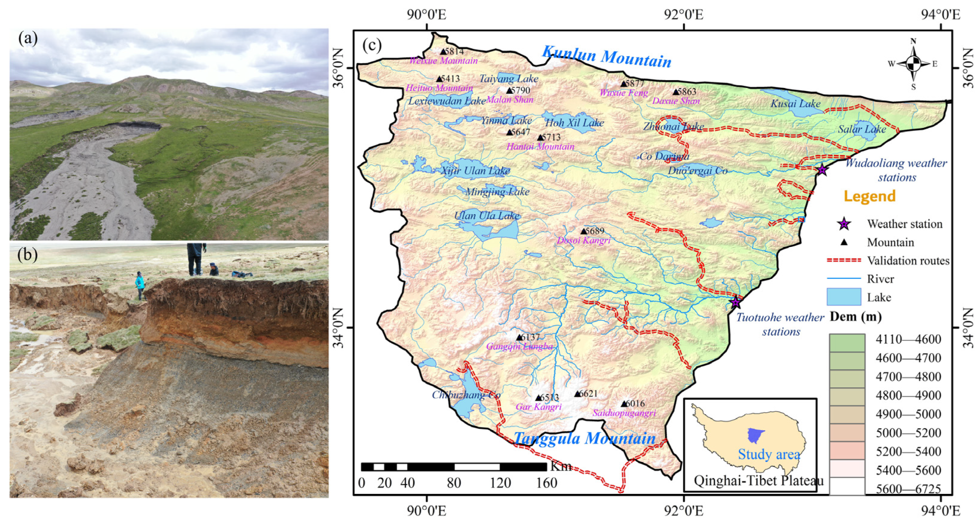
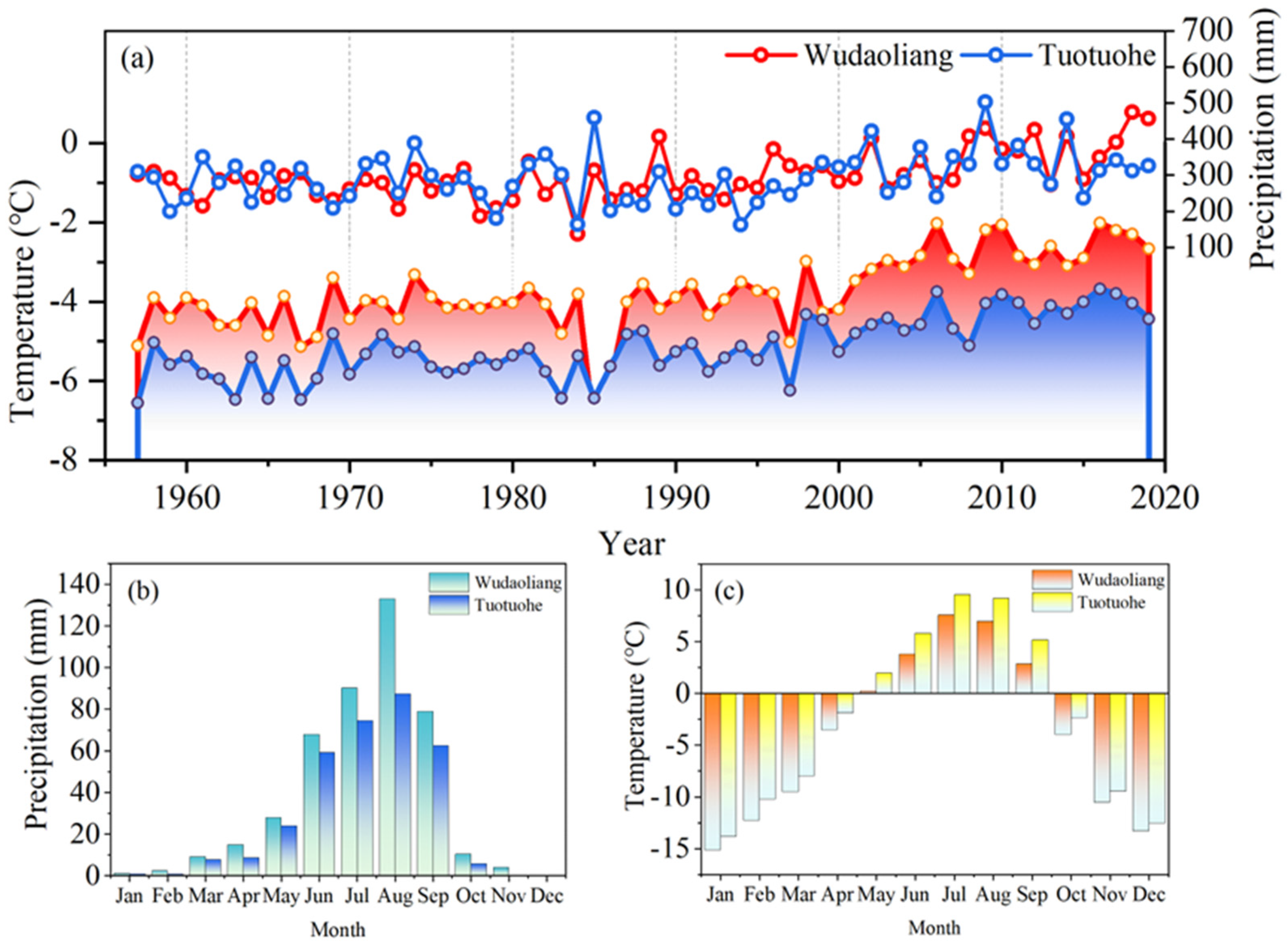
2.1. Study Area

The article tracked thaw slump activity in the hinterland of the plateau where the area is 83,000 km². The northern boundary extends to the middle parts of the Kunlun Mountains, while the southern boundary reaches the Tanggula Mountains. The westernmost boundary extends to the Tibet Autonomous Region, and the Qinghai–Tibet Highway runs along the easternmost boundary from south to north (Figure 1c). The study area is characterized by higher elevations at both the northern and southern ends and lower elevations in the middle, being minimally affected by river traceability erosion resulting from the substantial uplift of the QTP. The area is rich in surface water, with over hundreds of densely distributed large lakes (each with an area greater than 1 km²), as well as the presence of the Tuotuo River and the Chumaer River.

The climate of the plateau is cold and dry. Two official climate stations are situated along the QTH (http://cdc.cma.gov.cn, accessed on 6 June 2021): Wudaoliang (1957–present) in the northern region (93.08°E, 35.22°N, and 4612 m asl) and Tuotuohe (1957–present) in the intermediate section (92.43°E, 34.22°N, and 4533 m asl). The mean annual air temperatures from 1957 to 2019 at the Wudaoliang and Tuotuohe weather stations were −5.1 °C and −3.8 °C, with annual precipitation totals of 299 mm and 293 mm during the same period, over 90% of which falls as precipitation [42]. The climate is colder in the westernmost region, with the lowest annual mean air temperature recorded at −10 °C in early records [43]. January is the coldest month of the year, while July is the warmest, with a temperature difference exceeding 20 °C (Figure 2).

Three vegetation types cover more than 70% of the area, with alpine grassland being the predominant type, mainly distributed in the central and eastern areas, accounting for approximately 50% of the total area. The main plant species include Stipa purpurea, Carex moorcroftii, Littledalea racemosa, and Poa alpigena etc. Alpine meadows are mainly distributed on the northern slope of Tanggula Mountain, as well as on the foothills and concave lands of the central and eastern areas, which are conducive to the accumulation of snow and water, covering approximately 15% of the total area. The main plant species in alpine meadows include Kobresia pygmaea, Androsace tanggulashanensis, Elymus nutans Griseb., Kobresia littledalei C. B. Clarke, Puccinellia distans, etc. Alpine desert is primarily distributed at the base of shrinking or dry lakes and the lower parts of alluvial fans, with the main plant species being Ceratoides compacta. The high elevation and harsh climatic conditions result in a fragile ecosystem. There are no trees, and most plants are <15 cm in height, with a very short growing season. Wind erosion has led to an expansion of the area covered by bare ground and sparse vegetation [44]. The loose soils of the alpine steppe and alpine meadows are highly dry and prone to erosion from runoff, leading to desertification and loss of soil and water [43].

The study area is located within the zone of continuous permafrost, with a continuity exceeding 90% [45]. Reports of western permafrost are scarce, with more records from the east along the QTH. In small undulating mountains and high-altitude hilly areas with an altitude over 5000 m, the mean annual ground temperature approaches −4 °C, and the permafrost thickness exceeds 130 m. In most high plateaus or basins, the annual mean ground temperature exceeds −1.5 °C, and the permafrost thickness is less than 70 m [11]. The top 2–3 m of the permafrost layer contain ice-rich ground, with a maximum ground ice content of 70% [44]. Typically, the active layer thickness ranges from 2 to 3 m.

2.2. Image Data Acquisition and Processes

Data from three time periods to visually assess changes in thaw slumps in the hinterland of the QTP. Due to the relatively small scale of thaw slumps in the study area, high-resolution image data are required for accurate information extraction. The Keyhole satellite is an advanced optical imaging reconnaissance satellite that has evolved from the first satellite, KH1, launched in 1959, to the current KH12. The Keyhole data are characterized by their early imaging time and high resolution. In this study, a total of 117 full-color Keyhole images covering the study area from 1968 to 1970 were acquired from the USGS website (https://earthexplorer.usgs.gov, accessed on 8 September 2021). The image resolutions are 2.7 m for the KH4A satellite and 1.8 m for the KH4B satellite, respectively (Figure 3a).

The original Keyhole data downloaded were digitized from film to produce image files lacking spatial information, including geographic coordinates and a projection system. Because the images have black film edges and overlapping areas between them, cutting and splicing are necessary prior to image processing. Subsequently, the information enhancement processing steps, including image filtering, sharpening, and gray scale stretching, are implemented to emphasize the geomorphic information in the image. Lastly, the Keyhole image was matched to the geographical features image by selecting a sufficient number of control points and achieving uniform distribution whenever possible. The image was generated after undergoing three convolutional affine transformations.

The data from the second period consist of a compilation of approximately 50,000 frames of orthophoto images taken between 2006 and 2009, comprising various satellite images such as Spot5, IKONOS, and Resource 2. The image resolutions vary between 2.5 and 5.0 m for different satellite data. A total of 246 images were sourced from the Geospace and Natural Resources Big Data Center of Qinghai Province, accessed through the National Geographic Information Resources Catalogue Service System (https://www.webmap.cn, accessed on 15 November 2021). The data underwent processing steps including registration, orthorectification, and image fusion, as shown in Figure 3b.

The data from the third period comprises the Gaofen satellite images (abbreviated as GF) taken between 2018 and 2019. The GF satellite is the first Chinese optical remote sensing satellite to achieve a spatial resolution of less than 1 m. Spanning from Gaofen No.1 (GF-1) in 2013 to Gaofen No.14 (GF-14) in 2020, the GF image provides submeter-level spatial resolution, high positioning accuracy, and rapid attitude mobility. In this study, 130 GF images with minimal cloud and snow cover were obtained from the Gansu Data and Application Center (Gansu Gaofeng Center). These data encompass the GF-1, GF-2, GF-6, and ZY-3 satellite products, with respective resolutions of 2 m, 0.8 m, 2 m, and 2.1 m, as illustrated in Figure 3c.

Based on the Titan Supercomputer Platform (Titan Image), the GF data are utilized for performing tasks such as registration, multispectral and panchromatic image fusion, as well as RPC orthorectification. To preserve the rich information of the multispectral image, enhancements are made to the image resolution and texture information in order to ensure translation accuracy. The digital elevation model (DEM) data from the Shuttle Radar Topography Mission (SRTM) are utilized for extracting the topographic information of the study area. The terrain product data from the SRTM system are derived from space radar image data, featuring a coverage rate of over 80% and a resolution of 30 m. The data have undergone multiple revisions and are currently available as version 4.1, downloadable from the official USGS website (https://earthexplorer.usgs.gov, accessed on 8 September 2021).

2.3. Visual Interpretation and Validity Verification

In this study, the thaw slump area and quantity were extracted artificially by visual interpretation. Visual interpretation is widely used to extract surface information based on the morphology, texture, shadow, tone, and other features of the ground in remote sensing images, performed by experienced interpreters [46,47]. These interpretation results are frequently utilized to validate the accuracy of machine interpretation, which has not been surpassed in accuracy by other methods. Thaw slumps in the study area typically exhibit elongated strip-like, bifurcated, and tongue-like forms [48], creating distinct contour boundaries with the surrounding area due to the displacement of the active layer and the disruption of landform integrity. Following the displacement of the sliding body, the underlying ice beneath the active layer becomes exposed, leading to differences in soil water content and coverage between the collapsed area and the surrounding land (Figure 1a,b). Based on the shape, tone, and texture characteristics of thaw slumps in remote sensing images, their area and quantity were digitized using ArcMap 10.2 software.

Validating the interpretation results is a crucial process for assessing accuracy, including the validation of each thaw slump’s size and the total quantity of thaw slumps. The validation of the total quantity was conducted through three field surveys in specific regions from January 2021 to September 2022 (Figure 1c). During the field investigation in accessible regions, a total of 263 thaw slumps were identified, with 225 of them being accurately interpreted from the GF image of the same region. The overall statistical results indicate that the interpreted number of thaw slumps is slightly lower than the actual number, with an accuracy rate of approximately 85.6%. This discrepancy can be attributed to the fact that the image data were from 2018 to 2019, whereas the actual investigation took place in 2021~2022. It is possible that some new thaw slumps occurred in 2020–2022, or there were individual misinterpretations in the image.

The validation of each individual thaw slump area was conducted by comparing the interpreted area with the area in aerial photographs. In January 2021, aerial photographs of 12 thaw slumps in a local region were captured using an unmanned aerial vehicle (UAV) with a resolution of 0.1 m. Subsequently, the aerial images were processed to create digital orthophoto images (DOM). Using the DOM, the actual area of the thaw slumps was extracted and compared with the interpreted area from the GF image. This discrepancy may be due to the ongoing expansion of the thaw slumps or biases in the interpretation process. During the area interpretation process, efforts were made to account for the collapsing edges. However, limitations in the image quality of certain areas led to biased interpretation results, which were minimized as much as possible. Overall statistics indicate that the interpreted area is slightly smaller than the actual area, with an accuracy rate of approximately 97.5%.

2.4. The Informativeness Method and the Random Forest Principle

The occurrence and evolution of geological disasters are the result of the comprehensive interaction of various factors, with differences in the contribution of each factor. The information quantity model determines the information value of each evaluation index by statistically analyzing the distribution of occurred geological disasters in each evaluation index level and predicts the susceptibility of geological disasters in the research area. This method is highly reliable [49]. Therefore, various factors affecting the occurrence of geological disasters are taken as evaluation indicators. By calculating the frequency of known disaster points within each evaluation index level to determine the amount of information, the information values for each evaluation index are then superimposed to assess the susceptibility of disasters in the area. The formula for calculating the information quantity value is as follows:

$$\mathrm{I}\left(x_i\right)=\ln {\displaystyle \frac{S_i/A_i}{S/A}}\hspace{1em}\hspace{1em}\mathrm{i}=1,2,\dots ,\mathrm{n},$$

(1)

In this study, I denotes the predictive value of information quantity for the evaluation indicators in the research area. $S_i$ represents the geological disaster area distributed under the i-th class level of the x evaluation indicator, while $A_i$ stands for the number of geological disasters at the i-th class level of the x evaluation indicator. S denotes the total area of the research region, and A represents the total number of geological disasters within the research area.

Random forest is a classification method based on the integration of multiple decision trees. It involves the repeated random extraction of training samples for each decision tree from the training set to determine the optimal classification results and assess the importance of evaluation indicators, thus avoiding overfitting [44]. It possesses a high degree of objectivity. The linear weighted formula is as follows:

$$\mathrm{y}={\sum }_{j=1}^m{P}_{j}I(x_j),$$

(2)

where y represents the comprehensive information quantity, m denotes the number of evaluation indicators, and $P_j$ signifies the weighting coefficient for the evaluation indicator $x_j$.

The factors influencing the development of thaw slumps are numerous, encompassing both natural and anthropogenic disturbances. Natural factors include regional-scale climate variations such as persistent climate warming, intense short-term rainfall, thermal erosion induced by rivers and lakes, changes in land surface cover, as well as forest wildfires reported in the Arctic region [50]. Upon comprehensive field survey analysis, it was determined that the proportion of thaw slumps caused by disturbances from rivers, lakes, and human excavation on the Hoh Xil area is relatively small, accounting for approximately less than 10% of the total. The majority of occurrences are derived from the sliding and evolution of permafrost layers in hilly and mountainous gentle slope areas under natural conditions. Therefore, six factors, including slope (31.9% of thaw slumps at 4–6°), aspect (north- and northeast-facing slopes host 58.8% of thaw slumps), elevation (40.2% of thaw slumps at 4700–4800 m), annual mean temperature (86% of slumps occur at −6 to −4 °C), annual precipitation (81.8% of slumps arise with 300–400 mm/a), and ground ice content (36.2% in sediment-rich permafrost zones), were selected as evaluation indicators (Figure 4). Concurrently, the distribution quantity and area of thaw slumps under each evaluation indicator were recorded, and the information quantity values for each segment of the evaluation indicators were statistically analyzed according to Equation (1), completing the information quantity table.

3. Results

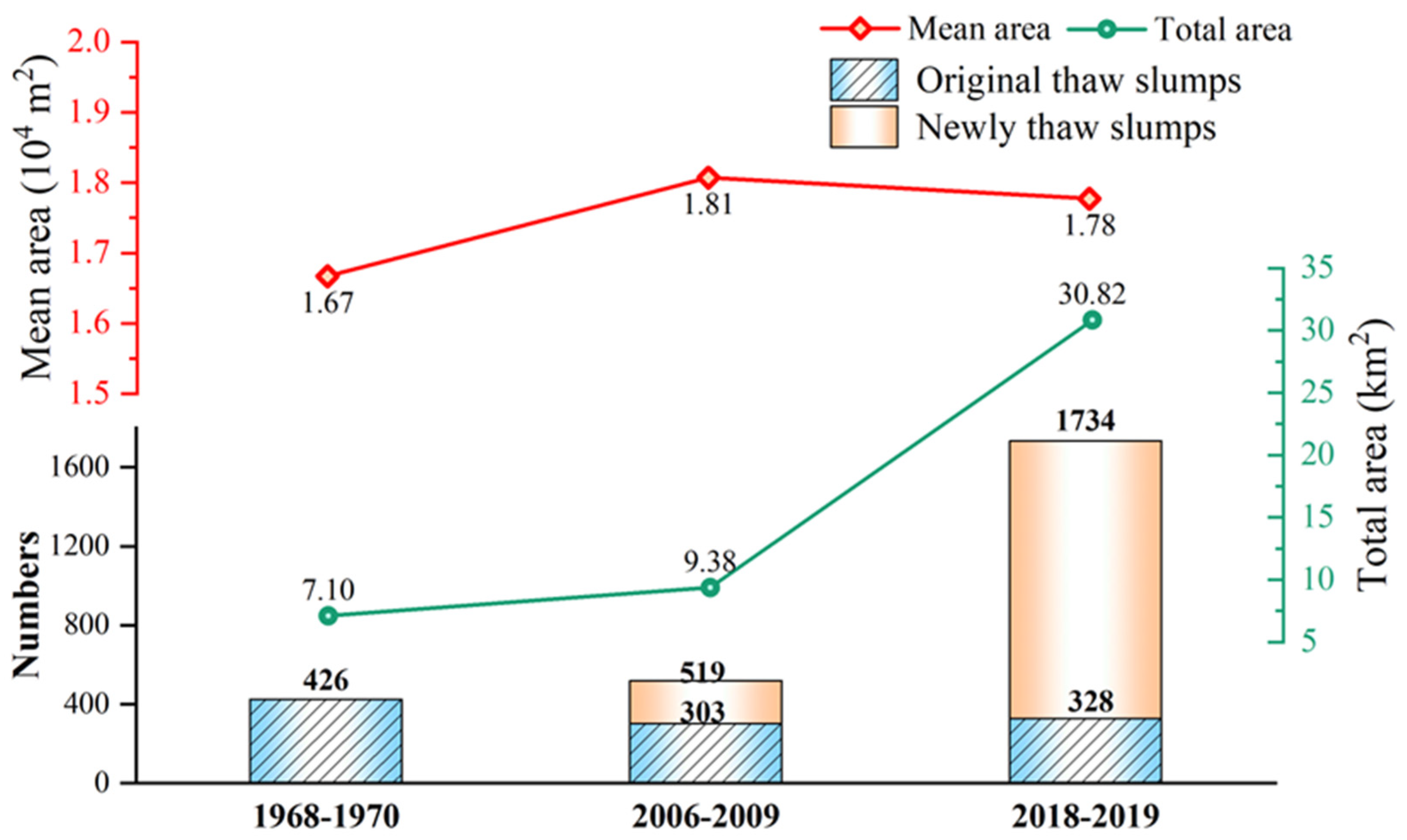
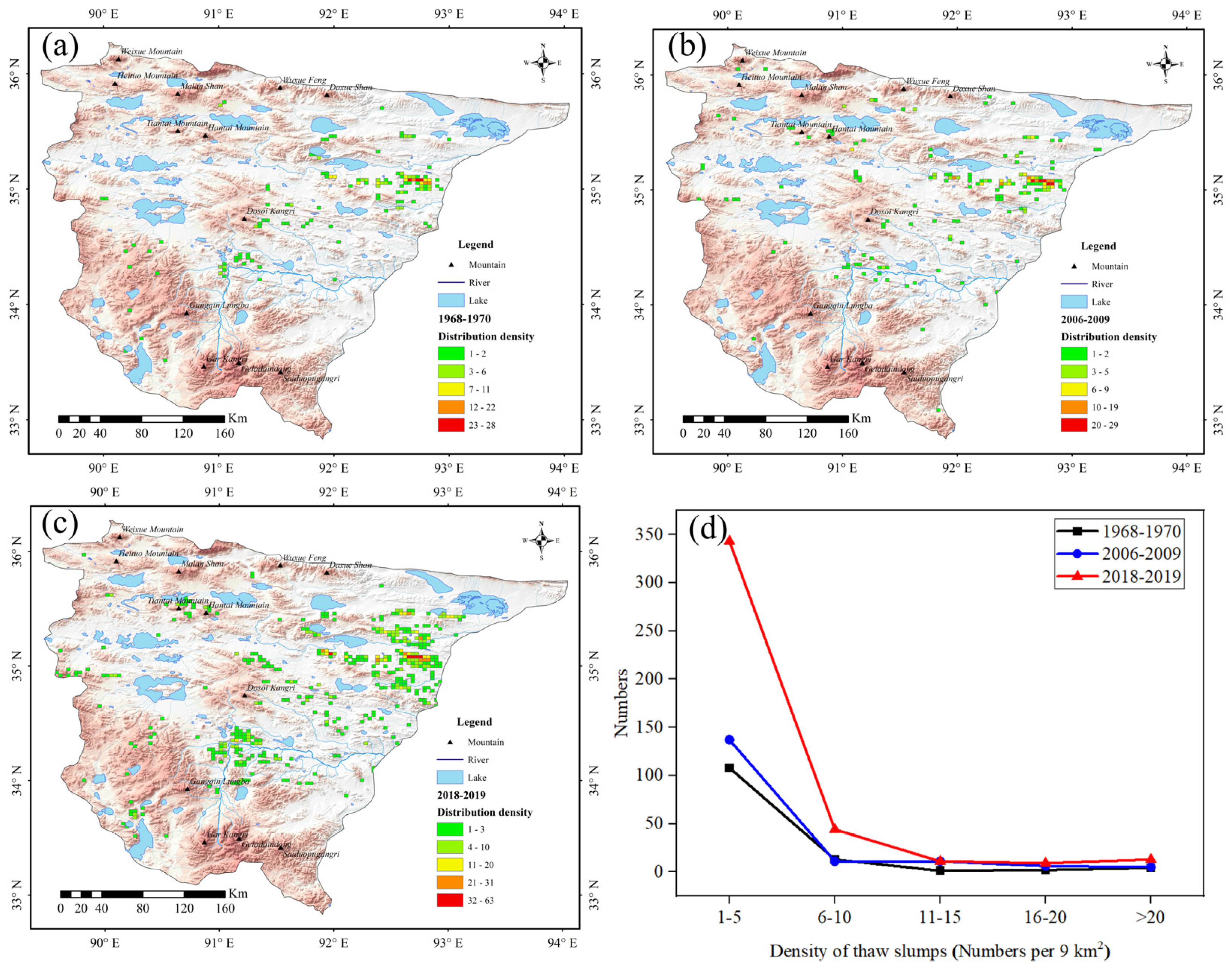
3.1. Changes in Thaw Slump Activity in Past 60 Years

This article identifies a significant increase in both the area and the number of thaw slump activities through images from the three periods spanning from 1960 to 2019. Approximately 426 active thaw slumps were identified in the entire study area in 1960 (Figure 5), covering a total area of 7.1 km². Over the next four decades, about 216 new thaw slumps were activated. Including 303 cases that continued to be active in the early stage, a total of 519 thaw slumps were identified in 2006, covering a total area of 9.38 km². In comparison to the period from 1960 to 2006, the number and area of active thaw slumps increased by 1.2- and 1.3-fold, respectively (Figure 5). By 2019, the total number of thaw slumps reached 1734, covering a total area of 30.82 km². In contrast to 1960, the number and area of active thaw slumps increased by 4- and 3-fold, respectively. Particularly, from 2006 to 2019, there was a significant increase in thaw slumping, with over 1200 new thaw slumps initiated in 2019 at an annual expansion rate of over 5.1 km²/a.

Approximately 10% of the thaw slumps present in 1960 continued to expand until 2006, owing to their initially larger scope and encompassing the early range of thaw slump. Conversely, the perimeters of nearly 90% of the thaw slumps from 1960 had become indistinct by this time, and their image characteristics no longer corresponded to those of a thaw slump. The surfaces of these inactive thaw slumps had seen vegetation growth, and their ridge-like sliding walls had been leveled due to long-term weathering from wind and rainfall. Based on these observations, the active period for most thaw slumps in the QTP hinterland spans approximately 30–40 years. A minority of these may exhibit a more extended active period, attributable to the specific conditions of ground ice and terrain.

The area of each thaw slump varied across different periods. In 1960, most thaw slumps were small in area, with almost none exceeding 20,000 m² and an average size of 1.67 × 10⁴ m². By 2006, the area of the initial 10% of thaw slumps had expanded, with the maximum area reaching approximately 15,000 m². The area of the 450 new thaw slumps ranged mainly from 10,000 to 20,000 m², with an average size of 1.81 × 10⁴ m². In 2019, results showed that out of 1734 thaw slumps, 469 (27%) were mainly less than 5000 m². Although the proportion was higher, these smaller thaw slumps accounted for only 4.3% of the total area. Thaw slumps ranging from 5000 to 10,000 m² accounted for 22.3% in number and 9.1% in area (Figure 5). The largest single thaw slump had an area of 20,000 m², comprising several laterally conjoined thaw slumps on the same slope, extending along a gentle slope for 1.5 km. These variations reflect the formation of numerous small thaw slumps during major initiation events and their subsequent enlargement over time.

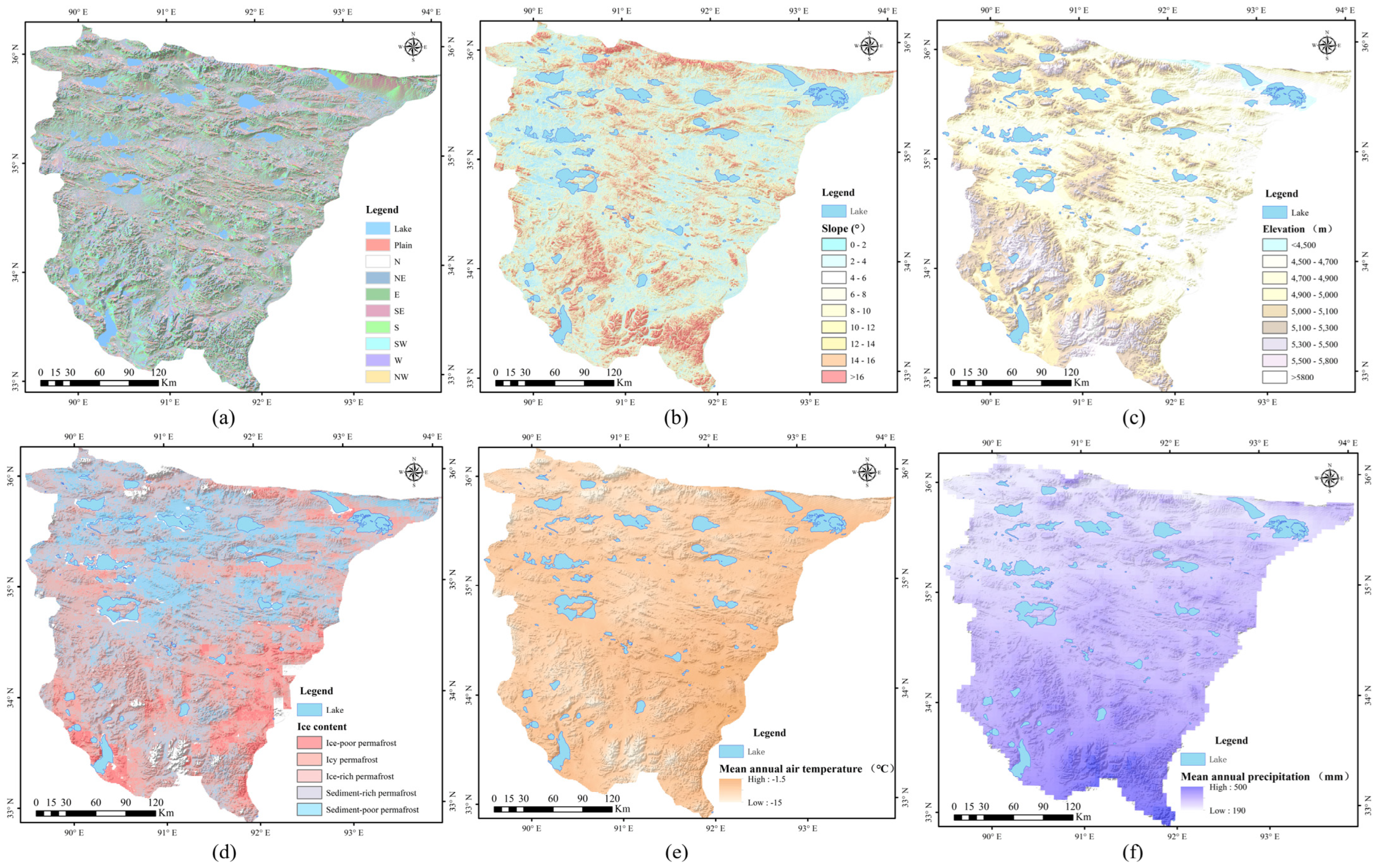
3.2. Spatial Distribution of the Thaw Slumps

The distribution of thaw slumps within the study area is notably uneven. To investigate the degree of concentration of thaw slumps, the study area was segmented into a grid of 3 km × 3 km cells, and the distribution density of thermal thaw slumps for each period was separately quantified (Figure 6). Statistical results indicate that the spatial distribution of thaw slumps primarily concentrates around the central and eastern mountainous regions of the Hoh Xil area. From 1968 to 1970, thaw slumps were predominantly found in the vicinity of the western side of the Hongliang River and the Beilu River, with a minor presence near Maqu Township (Figure 6a). Between 2006 and 2009, the development range of thermal thaw slumps expanded, extending towards the western region of Hoh Xil, with an increased distribution density along the Hongliang River (Figure 6b). The high-resolution imagery results from 2018 to 2019 (Figure 6c) demonstrate a substantial expansion in both the quantity and spatial distribution of thermal thaw slumps. Aggregation areas of thermal thaw slumps formed on the western side of the Hongliang River in the eastern part of Hoh Xil, around the Beilu River, from Wudaoliang Town to Cuodarijima and from the northern slope of Hoh Xil Mountain to Zhuonai Lake. The surroundings of Maqu Township and Sewu Township also became concentrated development areas for thaw slumps. A small number of thaw slumps developed around Hoh Xil Lake and Ulan Wulan Lake.

The entire Hoh Xil region has been divided into 9489 grid cells, each measuring 3 km by 3 km. Among these, 128 cells, constituting 1.3% of the total area, were identified as thaw slump development areas from 1968 to 1970. From 2006 to 2009, the number of such areas increased to 159, accounting for 1.7% of the total area. In 2018 and 2019, the number of cells with thaw slumps rose dramatically to 420, representing a significant 4.4% of the total area. According to the thaw slump distribution density statistics (Figure 6d), the majority of cells developed between 1 and 5 thaw slumps per 9 km². Specifically, in 1970, 108 cells (84%) developed 1–5 slumps, in 2006, the number was 137 cells (86%), and in 2018, it was 343 cells (82%). The number of thaw slumps exceeding six in a 9 km² cell was nearly consistent across the three periods. The maximum number of thaw slumps developed in a single 9 km² cell was 28 in 1970, 29 in 2006, and reached a peak of 63 in 2019.

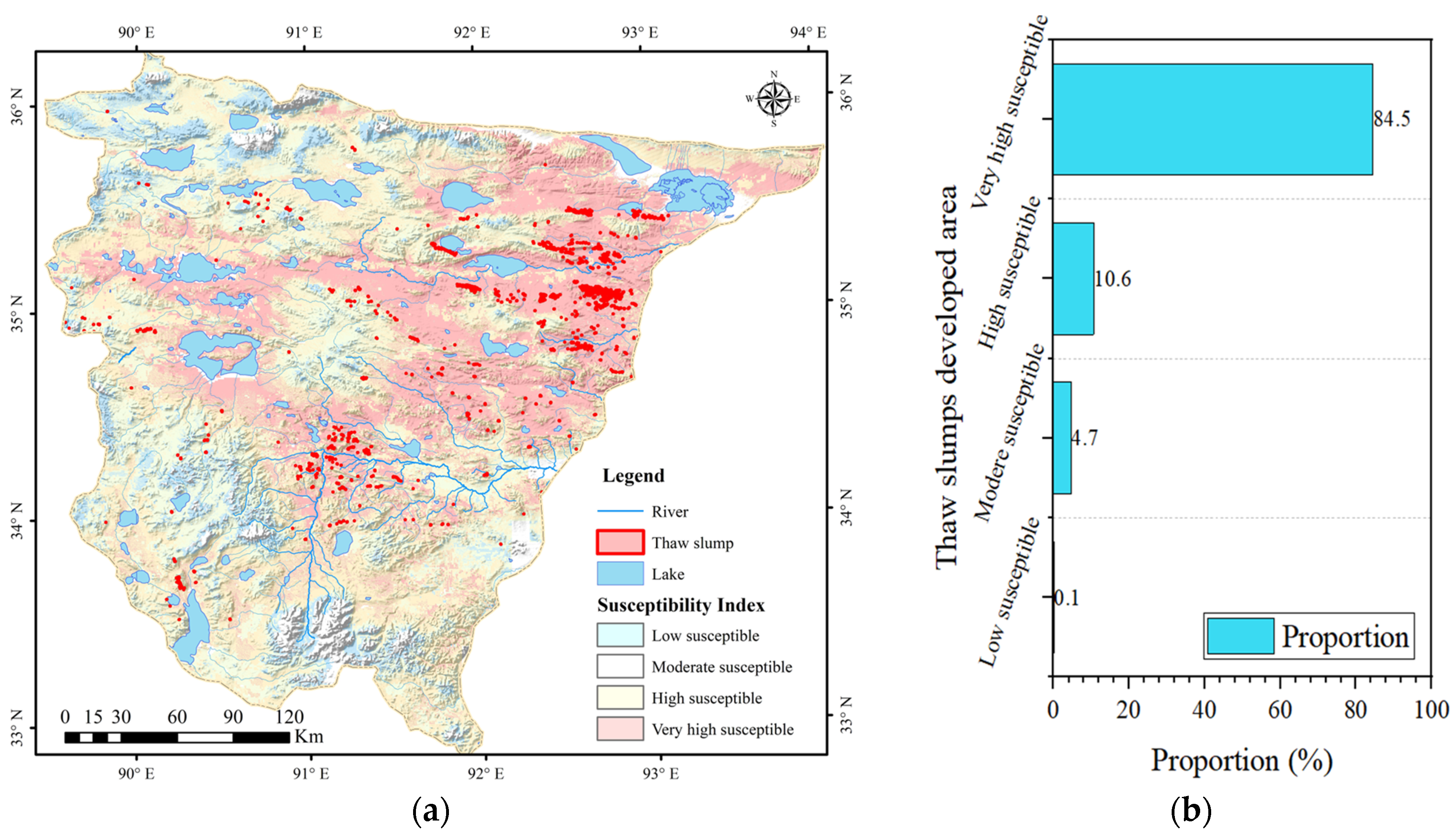
3.3. Susceptibility Assessment of Thaw Slumps

The sample set was derived from the interpretation of high-resolution imagery from 2018 to 2019, comprising 1734 thermal thaw slump areas (n = 1734) and a randomly selected 1700 non-thaw slump areas (n = 3434). The Random Forest training results reveal that among various evaluation indicators, elevation carries the greatest importance, followed by annual mean temperature, precipitation, slope direction, slope gradient, and ground ice content. A random selection of 85% of this data was utilized as the training sample, with the remaining serving as the test sample. The training test results indicate that when the number of classification trees is one, the model error tends to stabilize once the decision tree count exceeds 100. The accuracy of the training sample set remains steady at 81%, and the prediction sample set accuracy remains stable at 76%. These results demonstrate that the model parameters are suitable, stable, and reliable. The high weightage of elevation is primarily due to the fact that various natural factors in plateau regions closely correlate with altitude, significantly determining the distribution of water-heat and permafrost. Although subterranean ice content serves as a crucial precondition for the development of thermal thaw slumps, its weightage relatively small. This is mainly because Hoh Xil is replete with high-temperature, high-altitude permafrost, well-developed subterranean ice, and most areas satisfy the subterranean ice conditions required for thermal thaw slumps, resulting in minimal regional differences and thus a lower weightage for this indicator.

Utilizing the raster overlay analysis function of ArcGIS, the comprehensive information values of the entire research area were obtained by conducting a weighted statistical analysis of the weight maps of each evaluation indicator and the information content values in

Table 1. Classification of information values.

Factors	Classification	Information Value	Factors	Classification	Information Value
Elevation (m)	<4500	-	Slope (°)	0–2	−0.616333
	4500–4600	0.041871		2–4	−0.180810
	4600–4700	0.359353		4–6	0.262187
	4700–4800	1.168563		6–8	0.348616
	4800–4900	0.476836		8–10	0.451103
	4900–5000	−0.747066		10–12	0.118902
	5000–5100	−1.105579		12–14	−0.309901
	5100–5200	−1.605407		14–16	−0.332266
	5300–5400	−2.429923		>16	−1.041154
	5400–5500	−2.077762	Slope aspect	N	0.540414
Mean annual air temperature (°C)	<−8	−3.754438		NE	0.538344
	−7~−8	−1.718537		E	0.026313
	−6~−7	−1.182438		SE	−0.506935
	−5~−6	0.325547		S	−0.680544
	−4~−5	0.673817		SW	−0.693052
	−3~−4	−0.508229		W	−0.215437
	−1.7~−3	−1.989411	Ice content	Ice-poor	−1.152652
Mean annual precipitation (mm)	200–300	−1.788738		Icy	−0.206302
	300–400	0.224823		Ice-rich	−0.074456
	400–500	0.020186		Sediment-rich	0.146778
	500–600	−3.262990		Sediment-poor	0.225083

, according to Equation (2). The natural breakpoint method, employing a clustering mindset and ensuring a similar scope and number of elements in each group, was used to divide the entire region into four categories: extremely high susceptibility zones, high susceptibility zones, medium susceptibility zones, and low susceptibility zones. This led to the delineation of thermal thaw slump susceptibility zones in the Hoh Xil region. Among these, the areas around the eastern part of Hoh Xil extending to the Qinghai–Tibet highway, the Western Jin Wulan Lake, Ulan Ula Lake, and Maqu Township are classified as extremely high susceptibility zones, accounting for approximately 26% of the entire evaluated area. The regions surrounding these high susceptibility zones, areas below an altitude of 5000 m with developed water systems, are deemed high susceptibility zones, accounting for about 36% of the entire evaluated area. The moderate and low susceptibility zones primarily cover the mountainous regions in the central and western parts of Hoh Xil at altitudes exceeding 5000 m, making up approximately 38% of the entire evaluated area (Figure 7a). The validation of the entire simulation results revealed that the proportion of thermal thaw slumps in the very high susceptible zones is 84.5%, and in the high susceptible zones, it is 10.6%, indicating that the evaluation results of the susceptible zones are quite satisfactory (Figure 7b). This study also suggests that there is a significant probability of thaw slump development in 26% of the Hoh Xil region.

4. Discussion

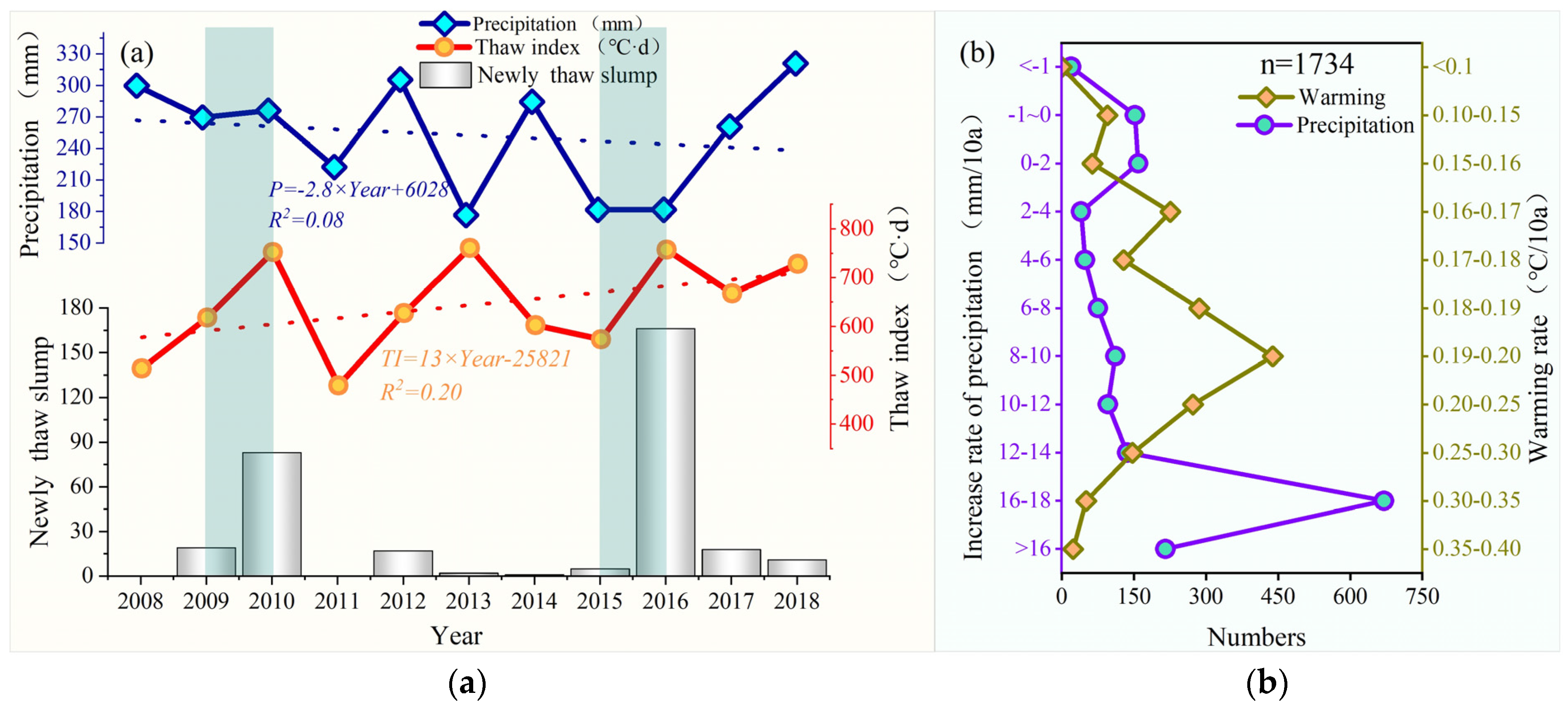
4.1. Relationship Between Thaw Slump and Warming Climate and Precipitation

The increase of thaw slumps, both in terms of quantity and area, is markedly evident in the hinterland of the QTP. This phenomenon is intrinsically associated with the thawing of ice-rich permafrost, a process correlated with escalating air temperatures and increased precipitation during the warm season (June–September). Studies have indicated that since 1979, the Arctic’s air temperature has been warming at nearly four times the global rate [51]. Similarly, the rise in air temperature and precipitation on the plateau has been significant, approximately twice as fast as the global average [42,52]. Data from three official weather stations on the periphery of the study area revealed a notably accelerated increase in air temperature post-2000 compared to the period before 2000 (Figure 2). Although the average warming rate was double the global average, the increase in the warmest monthly mean air temperature (July or August) from 2000 to 2019 was about 0.6 °C/decade, roughly four times the global average. While the yearly data were not obtained for the number of thaw slumps from 1960 to 2019, image analysis from two time periods suggests that the growth rate of new thaw slumps between 1960 and 2006 was relatively low, at approximately 1.3 times. This aligns with the gradual increase in air temperature during the warmest months over this period. However, between 2006 and 2019, the quantity of thaw slumps nearly tripled, and the area quadrupled, mirroring the drastic temperature increase during this time. The summer rainfall variation on the Qinghai–Tibet Plateau was not as pronounced as the rise in air temperature and showed a trend toward zero increase before 2000 (Figure 2). However, post-2000, summer rainfall also saw a significant upswing, with an average increase rate of about 6 mm/year. The sharp rise in both air temperature and precipitation during the warm season since 2000 has been a key driving force behind the rapid surge in thaw slumps. The activation of more thaw slumps does not necessarily coincide with extremely warm air temperatures and heavy rainfall in the same year; rather, it typically peaks one to two years after such extreme climatic events, leading to the eruption of thermokarst landforms (thaw slump, thermokarst lake, and gelifluction, etc.).

In regions devoid of human interference, the development of thaw slumps is significantly correlated with extreme summer temperatures and intense precipitation [22,29]. Combining the data on the development of thaw slumps in the Beiluhe Basin from 2008 to 2018, as recorded by Luo et al. [29], an analysis was conducted on the correlation between the development of thaw slumps and the thaw index and warm-season precipitation. In terms of the increase in the number of newly developed thaw slumps, there has been a consistent upward trend over the past decade, punctuated by two notable surges in 2010, with an increase of 83 sites, and 2016, with an increase of 166 sites. During the period from 2008 to 2010, the temperature rose continuously, with the thawing index increasing by 238.4 °C·d. Additionally, there was a temperature increase in 2015–2016, with the melting index rising by 183.9 °C·d (Figure 8a). This clearly indicates that the quantity of thaw slumps exhibits a pronounced feedback response to the rapid rise in summer temperatures. Lacell et al. [53] argue that the relationship between thaw slumps and summer temperatures is not always directly proportional. An analysis of the temperature increase and precipitation change rates in the entire study area’s thaw slump occurrence zones revealed a warming trend in the climate of all these areas. The temperature increase rate for 25% of the slump development areas ranged from 0.19 to 0.20 °C/decade, while 61% of the thaw slump occurrence zone areas had a temperature increase rate between 0.18 and 0.25 °C/decade. Concerning precipitation increase, approximately 10% of the thaw slump occurrence areas experienced reduced precipitation and warming temperature, while more than 60% of these areas exhibited an annual average precipitation increase rate exceeding 12 mm/decade (Figure 8b). This suggests that precipitation transfers surface heat to the upper layers of the permafrost, accelerating ground ice melting, increasing soil pore water pressure, and consequently elevating the speed of thaw slump development. Thus, the occurrence of thaw slumps was induced by the combined influence of temperature and precipitation.

4.2. Driving Mechanism of Thaw Slump

Statistical analysis revealed that in 2019, thaw slump occurrences were most frequently initiated on natural slopes (74%), along the lakeshore (25%), and near the road (just 1%). The analysis of environmental factors suggests that the occurrence of thaw slumps under these three conditions corresponds to distinct driving forces.

On the natural slope, distant from water bodies or human activities, the driving triggering factor is attributed to extreme climate, including warm air temperatures and heavy summer rainfall. This conclusion is not unsubstantiated, as a study on the sudden increase in thermokarst lakes in this region essentially confirmed that persistent climate warming and increased precipitation were the likely potential driving factors [33]. Similar studies in the Arctic permafrost region also showed that extremes in summer climate triggered thousands of thaw slumps [22]. In light of this induced mechanism, a model to describe the developmental process of thaw slump occurrences on natural slopes, based on sustained examination of several typical thaw slumps (Figure 1). First, the continual warming air temperature and increasing rainfall may result in the deepening active layer and long-term talik development between the bottom of the active layer and the top of the permafrost. This is fully supported by monitored data over the past 20 years on the QTP [54,55,56]. The melting of ground ice and thickening of taliks are accompanied by heat absorption and seepage at the ground surface. During this process, high pore water pressure and low effective shear strength within the saturated or oversaturated talik result in slope failure. Once the slope loses stability, the active layer slides along the fragile surface of the top permafrost. This process may occur instantly, causing the slope to tear apart and expose the subsurface ice at the headwall. Subsequently, the collapse process occurs over subsequent years, expanding the exposed area until the subsurface ice disappears. Therefore, the major initiator of thaw slump occurrences on slopes is a deepening thaw layer caused by the combination of warm air temperatures and heavy rainfall since the year 2000.

Although most thaw slump occurrences (about 2/3) were caused by the deepening of active layers, about 25% were linked to water bodies such as rivers or lakes. Extreme climate has accelerated the melting of glaciers, snow, and permafrost degradation, leading to an increase in water bodies on the QTP, including rising lake water levels and increased river flow [33,56]. During summer, when river flow increases, the water may erode or disturb the permafrost at river bends, leading to the initial melting of ground ice at these locations. The unsupported active layer starts to settle, and the ground surface was torn, resulting in slope failure similar to thaw slump occurrences on natural slopes (Figure 9a). The study area is located in the plateau interior, with many large lakes. Studies have shown that lake levels have significantly increased over the past few decades, including both large established lakes and newly formed thermokarst lakes [33,49]. On the slopes around the lakes, many thaw slumps were triggered due to factors such as wave action and thermal abrasion.

Thaw slumps, triggered by excavation or vibration from construction projects, currently account for a small proportion and were typically found on either side of major infrastructure projects. An illustrative example along the Qinghai–Tibet Highway in the 1990s exemplifies this process. During that period, excavation displaced surface soil, leaving a depression. Subsequently, a thaw slump became active for over 20 years. After 2010, the rate of expansion slowed and then stopped altogether until 2014 [30]. Currently, vegetation has begun to grow on the disturbed surface. While these types of thaw slumps are relatively few in number, they are typically found near highways and railways. A sharp increase of this thaw slump type is predicted in the future due to the growing human activity and construction projects (Figure 9b).

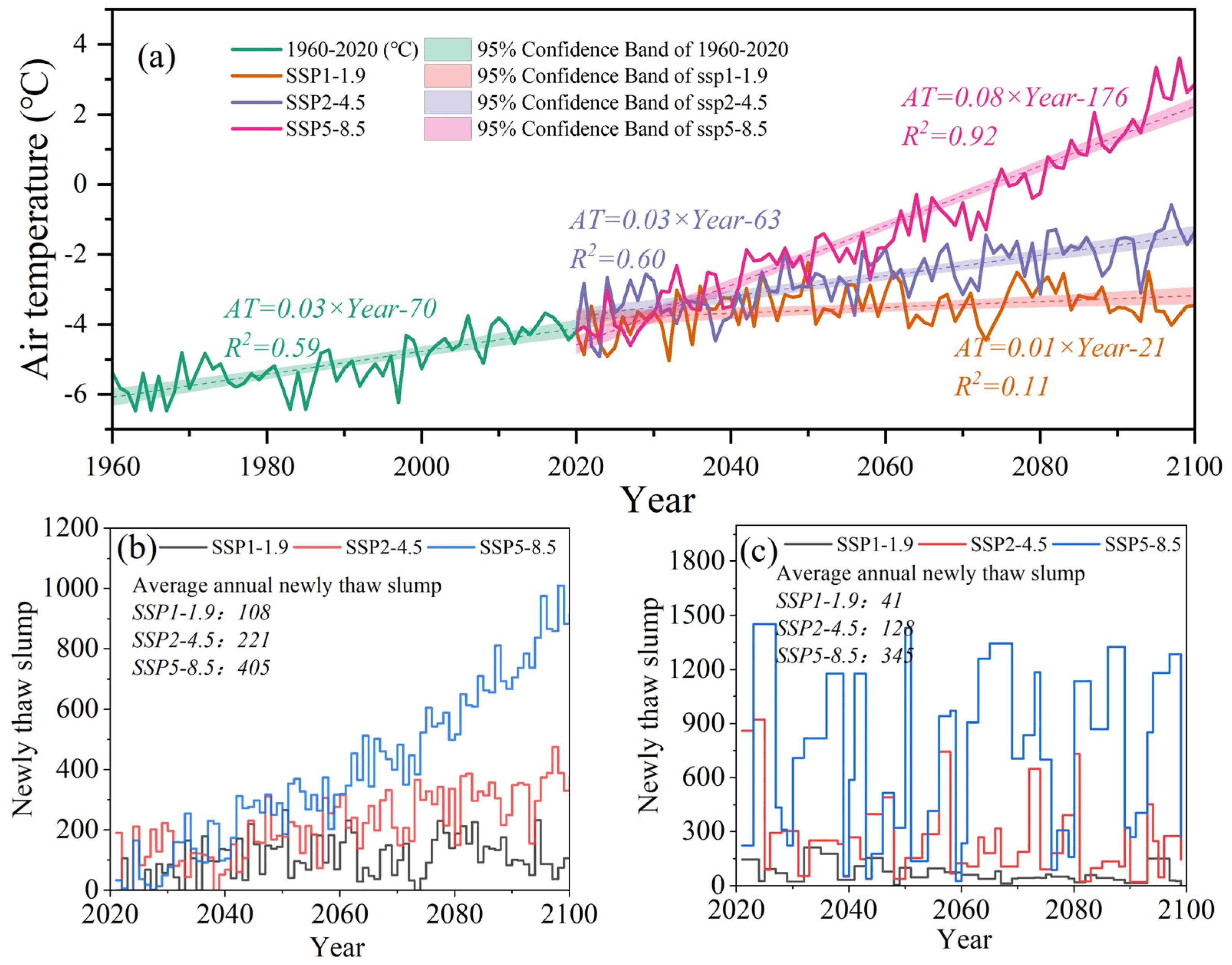
4.3. Future Trends in Thaw Slump Development

The widespread occurrence of thaw slump development is attributed to climate change. Within three distinct periods, the area affected by thaw slumps occupies less than 4.5% of the total area of the Hol Xil. Notably, the maximum density of thaw slumps within a 9 km² grid unit reached 63 occurrences during 2018–2019 (Figure 6). Calculated at an average area of 1.78 × 10⁴ m² per thaw slump, the developed area within the grid was approximately 1.12 km², representing approximately 12.5% of the grid’s total area. The distribution of thaw slumps, with its highest impact density, is lower than the findings of Lewkowicz and Way [22] in Banks Island, Canada, which reported a 17.3% density.

The spatial extent of thaw slumps development across the three periods has significantly expanded, closely linked to the pronounced rise in regional temperatures. Overall, there is no significant variation in precipitation levels across the QTP, and its relative impact is minimal [57]. Considering the cyclical nature of thaw slumps development, temperature data from 2021 to 2100 have been selected for analysis. The average annual temperature increase in the QTP from 1960 to 2020 was 0.03 °C/a. According to the EC-Earth model, the temperature warming rates from 2020 to 2100 are projected to be 0.01 °C/a, 0.03 °C/a, and 0.08 °C/a, respectively (Figure 10a). Based on the correlation study between the increase in thaw slumps occurrences and temperature by Luo et al. [33] on the Beiluhe Basin, together with the interpretation results from the three periods, the trend of thaw slumps development from 2020 to 2100 has been calculated. According to the growth calculations by Luo et al. [33], the minimum increase in thaw slumps occurrences per year in the QTP is projected to be 108 (SSP1-1.9), while the maximum is expected to reach 405 occurrences per year (SSP5-8.5) (Figure 10b). Furthermore, based on the interpretation results from the three periods, the predicted increase in thaw slumps occurrences from 2020 to 2100 is estimated to be 41 occurrences per year under SSP1-1.9, and 3-4.5 occurrences per year under ssp5-8.5 (Figure 10c). These two sets of results illustrate varying scenarios of thaw slumps development. Given that the interpretation by Luo et al. [33] was conducted in the Beiluhe Basin on the Hol Xil, where the density of occurrences is significantly higher than in the entire region of Hol Xil, it is deemed that their calculated results are overly optimistic. Nonetheless, both calculation methods indicate a sharp increase in future thaw slumps occurrences, which could potentially have a significant impact on the regional environment.

4.4. Disaster Effect Caused by Thaw Slump

Permafrost plays a crucial role in the cryospheric environment, acting as a water-resistant layer that preserves the moisture balance in the active layer and ensures ecosystem sustainability [58]. However, when a thaw slump is initiated and continues to develop on the surface, it leads to a range of environmental and engineering disaster risks, including surface exposure and ground ice melting (Figure 11).

The direct effect of the thaw slump is the destruction of the surface landscape pattern, resulting in the formation of the ‘psoriasis’ landform, significantly impacting the plateau landscape environment [59]. Conventional studies suggest that thaw slumps are relatively small. However, as the climate continues to warm, the development of massive thaw slumps, spanning 20 × 10⁴ m², will significantly impact local terrestrial surface environments (Figure 11a). The ecosystem on the QTP is exceptionally delicate, and surface exposure accelerates the degradation of high-altitude ecosystems. Prior to the occurrence of thaw slumps, vegetation thoroughly covered most slope surfaces in the area, but post-slump, the slopes became nearly barren [33]. The exposed soil experiences a decrease in retention force, accelerating the desertification process due to wind erosion during the spring and winter seasons [60]. However, the warming climate has resulted in both warm-humid and warm-dry conditions, indicating that the vegetation succession following thaw slumps can transition not only to desertification and grasslands, but can also give rise to shrubbery within the slump area (Figure 11b). This may be attributed to the rising ground temperatures in the thaw slump areas, causing permafrost disappearance and subsequent soil temperature elevation, creating favorable conditions for shrub growth.

Thaw slump events have resulted in the destruction of nearby buildings and their associated facilities. For instance, in 2018, a thaw slump at Fenghuo Mountain led to the destruction of the Qinghai–Tibet Railway fence and the accumulation of debris on the roadbed, posing significant hazards to road safety. While the Hoh Xil region is sparsely populated, there are sporadic pastoral inhabitants. Thaw slump events in certain areas also pose a safety risk to individuals in these pastoral areas. For example, during an investigation in Sewu Township, a residential area was identified where a substantial thawing and sliding process had developed on the slope, with the resultant mudflows posing a threat to several houses (Figure 11c). At the periphery of the QTP, in areas with steep inclines, the development of thaw slump events may trigger the occurrence of large-scale mudflows, thereby significantly impacting human habitation. For instance, the collapse behind the county seat of Qilian resulted in the formation of extensive mudflows, affecting the safety of Qilian County (Figure 11d).

In addition to prominent environmental effects such as water environment [61,62] and carbon release [19,63,64], thaw slump events can also trigger major disasters, forming a chain of calamities. During field investigations, large-scale permafrost landslides were observed on steep mountain slopes, with reduced mountain material at the upper part of the slope due to permafrost thaw, and deformation occurring in the lower part of the mountain, leading to the inference that the landslide may been induced by thaw slump (Figure 11e). Similarly, in steep regions, long-distance thaw slumps were likely to develop, carrying substantial sediment, leading to the obstruction of small streams (Figure 11f). Consequently, thaw slumps may harbor significant latent hazards.

5. Conclusions

This study conducted an interpretation of thaw slump distribution characteristics and spatiotemporal variation trends in the Hoh Xil area based on three periods of data: keyhole images of 1968–1970, the fractional images of 2006–2009, and the GF images of 2018–2019, combined with field surveys for validation. An assessment of the susceptibility to thaw slumping was performed using the random forest–information quantity method in the Hoh Xil area. The conclusions are as follows: Thaw slumps have been in a state of sustained development from 1968 to 2019, with the number and area of thaw slumps increasing threefold and twofold, respectively, over 40 years. Approximately 70% of the thaw slump events during the three periods were of a scale less than 2 × 10⁴ m², with 115 occurrences persisting from 1970 to 2019. Spatial variability is evident in the development of thaw slump, with concentrated distribution in the central and eastern parts of the Hoh Xil. The statistical results of thaw slump distribution density indicate a continuous increase in both the quantity and density of thaw slump, with the most frequent occurrence being 1–5 thaw slump events developing within a 9 km² grid, and in 2019, one grid witnessed the development of 63 thaw slump occurrences. The extremely high area for thaw slump in Hoh Xil encompasses approximately 26% of the entire region, reflecting around 36% of the total area. Overall, the eastern part of Hoh Xil exhibits a high susceptible to thaw slump developed. In this area, the development of thaw slump primarily occurs through three modes: temperature- and precipitation-induced, thermal erosion induced by rivers and lakes, and engineering disturbance. Future assessments of thaw slump development suggest a possible minimum of 41 and a maximum of 405 thaw slumps occurrences annually on the Hoh Xil. Under rapidly changing climatic conditions, apart from environmental risks, there also exists substantial potential risks associated with thaw slump, such as triggering large-scale landslides and debris flows. Therefore, it is imperative to conduct simulated assessments of thaw slumps throughout the entire plateau to address regional risks in the future.

References

1. Salzmann, N.; Frei, C.; Vidale, P.L.; Hoelzle, M. The application of Regional Climate Model output for the simulation of high-mountain permafrost scenarios. Glob. Planet. Change 2007, 56, 188–202. [Google Scholar] [CrossRef]
2. Lawrence, D.M.; Slater, A.G.; Romanovsky, V.E.; Nicolsky, D.J. Sensitivity of a model projection of near-surface permafrost degradation to soil column depth and representation of soil organic matter. J. Geophys. Res. 2008, 113, F02011. [Google Scholar] [CrossRef]
3. Schaphoff, S.; Heyder, U.; Ostberg, S.; Gerten, D.; Heinke, J.; Lucht, W. Contribution of permafrost soils to the global carbon budget. Environ. Res. Lett. 2013, 8, 014026. [Google Scholar] [CrossRef]
4. Marmy, A.; Salzmann, N.; Scherler, M.; Hauck, C. Permafrost model sensitivity to seasonal climate changes and extreme events in mountainous regions. Environ. Res. Lett. 2013, 8, 035048. [Google Scholar] [CrossRef]
5. Wang, Q.; Fan, X.; Wang, M. Recent warming amplification over high elevation regions across the globe. Clim. Dyn. 2014, 43, 87–101. [Google Scholar] [CrossRef]
6. Biskaborn, B.K.; Smith, S.L.; Noetzli, J.; Matthes, H.; Vieira, G.; Streletskiy, D.A.; Schoeneich, P.; Romanovsky, V.E.; Lewkowicz, A.G.; Abramov, A.; et al. Permafrost is warming at a global scale. Nat. Commun. 2019, 10, 264. [Google Scholar] [CrossRef]
7. Smith, S.L.; O’Neill, H.B.; Isaksen, K.; Noetzli, J.; Romanovsky, V.E. The changing thermal state of permafrost. Nat. Rev. Earth Environ. 2022, 3, 10–23. [Google Scholar] [CrossRef]
8. Cheng, G.D.; Wu, T.H. Responses of permafrost to climate change and their environmental significance, Qinghai-Tibet Plateau. J. Geophys. Res. Earth Surf. 2007, 112, 1–10. [Google Scholar] [CrossRef]
9. Jin, H.J.; Luo, D.L.; Wang, S.L.; Lü, L.Z.; Wu, J.C. Spatiotemporal variability of permafrost degradation on the Qinghai-Tibet Plateau. Sci. Cold Arid Reg. 2011, 3, 281–305. [Google Scholar]
10. Luo, D.; Jin, H.; Bensead, V.F.; Jin, X.; Li, X. Hydrothermal processes of near-surface warm permafrost in response to strong precipitation events in the Headwater Area of the Yellow River, Tibetan Plateau. Geoderma 2020, 376, 114531. [Google Scholar] [CrossRef]
11. Zhou, Y.W.; Guo, D.X.; Qiu, G.Q.; Cheng, G.D.; Li, S.D. Geocryology in China; Science Press: Beijing, China, 2000. [Google Scholar]
12. Ermolaev, M.M. Geological and Geomorphological Description of Bol’shoi Lyakhovskii Island; Trudy SOPS AN SSSR, Ser. 7; Publishing House of the Academy of Sciences of the USSR: Yakutsk, Russia, 1932. (In Russian) [Google Scholar]
13. Soloviev, P.A. Thermokarst phenomena and landforms due to frost heaving in Central Yakutia. Biul. Peryglac. 1973, 23, 135–155. (In Russian) [Google Scholar]
14. Kokelj, S.V.; Lantz, T.C.; Tunnicliffe, J.; Segal, R.; Lacelle, D. Climate-driven thaw of permafrost preserved glacial landscapes, northwestern Canada. Geology 2017, 45, 371–374. [Google Scholar] [CrossRef]
15. Lin, Z.; Niu, F.; Xu, Z.; Xu, J.; Wang, P. Thermal regime of a thermokarst lake and its influence on permafrost, Beiluhe Basin, Qinghai-Tibet Plateau. Permafr. Periglac. Process. 2010, 21, 315–324. [Google Scholar] [CrossRef]
16. Niu, F.; Luo, J.; Lin, Z.; Ma, W.; Lu, J. Development and thermal regime of a thaw slump in the Qinghai–Tibet Plateau. Cold Reg. Sci. Technol. 2012, 83–84, 131–138. [Google Scholar] [CrossRef]
17. Burn, C.R.; Lewkowicz, A.G. Canadian Landform Examples—17: Retrogressive thaw slumps. Can. Geogr. 1990, 34, 273–276. [Google Scholar] [CrossRef]
18. Matsuoka, N. Solifluction and mudflow on a limestone periglacial slope in the Swiss Alps: 14 years of monitoring. Permafr. Periglac. Process. 2010, 21, 219–240. [Google Scholar] [CrossRef]
19. Liljedahl, A.K.; Boike, J.; Daanen, R.P.; Fedorov, A.N.; Frost, G.V.; Grosse, G.; Hinzman, L.D.; Iijma, Y.; Jorgen-son, J.C.; Matveyeva, N.; et al. Pan-Arctic ice-wedge degradation in warming permafrost and its influence on tundra hydrology. Nat. Geosci. 2016, 9, 312–318. [Google Scholar] [CrossRef]
20. Fraser, R.H.; Kokelj, S.V.; Lantz, T.C.; McFarlane-Winchester, M.; Olthof, I.; Lacelle, D. Climate sensitivity of high Arctic permafrost terrain demonstrated by widespread ice-wedge thermokarst on Banks Island. Remote Sens. 2018, 10, 954. [Google Scholar] [CrossRef]
21. Gao, Z.Y.; Zhang, C.; Liu, W.; Niu, F.; Wang, Y.; Lin, Z.; Yin, G.; Ding, Z.; Shang, Y.; Luo, J. Extreme degradation of alpine wet meadow decelerates soil heat transfer by preserving soil organic matter on the Qinghai–Tibet Plateau. J. Hydrol. 2025, 653, 132748. [Google Scholar] [CrossRef]
22. Lewkowicz, A.G.; Way, R.G. Extremes of summer climate trigger thousands of thermokarst landslides in a High Arctic environment. Nat. Commun. 2019, 10, 1329. [Google Scholar] [CrossRef]
23. Lewkowicz, A.G. Dynamics of active-layer detachment failures, Fosheim Peninsula, Ellesmere Island, Nunavut, Canada. Permafr. Periglac. Process. 2007, 18, 89–103. [Google Scholar] [CrossRef]
24. Rudy, A.C.A.; Lamoureux, S.F.; Treitz, P.; Van Ewiijk, K.; Bonnaventure, P.P. Terrain controls and landscape-scale susceptibility modelling of active-layer detachments, Sabine Peninsula, Melville Island, Nunavut. Permafr. Periglac. Process. 2016, 28, 79–91. [Google Scholar] [CrossRef]
25. Borge, A.F.; Westermann, S.; Solheim, I.; Etzelmüller, B. Strong degradation of palsas and peat plateaus in northern Norway during the last 60 years. Cryosphere 2017, 11, 1–16. [Google Scholar] [CrossRef]
26. Mamet, S.D.; Chun, K.P.; Kershaw, G.G.L.; Loranty, M.M.; Kershaw, G.P. Recent increases in permafrost thaw rates and areal loss of palsas in the western Northwest Territories, Canada. Permafr. Periglac. Process. 2017, 28, 619–633. [Google Scholar] [CrossRef]
27. Schuur, E.A.G.; McGuire, A.D.; Schädel, C.; Grosse, G.; Harden, J.W.; Hayes, D.J.; Hugelius, G.; Koven, C.D.; Kuhry, P.; Lawrence, D.M.; et al. Climate change and the permafrost carbon feedback. Nature 2015, 520, 171–179. [Google Scholar] [CrossRef]
28. Mu, C.; Schuster, P.F.; Abbott, B.W.; Kang, S.; Guo, J.; Sun, S.; Wu, Q.; Zhang, T. Permafrost degradation enhances the risk of mercury release on Qinghai-Tibetan Plateau. Sci. Total Environ. 2019, 708, 135127. [Google Scholar] [CrossRef]
29. Luo, J.; Niu, F.; Lin, Z.; Liu, M.; Yin, G. Recent acceleration of thaw slumping in permafrost terrain of Qinghai-Tibet Plateau: An example from the Beiluhe Region. Geomorphology 2019, 341, 79–85. [Google Scholar] [CrossRef]
30. Niu, F.; Luo, J.; Lin, Z.; Fang, J.; Liu, M. Thaw-induced slope failures and stability analyses in permafrost regions of the Qinghai-Tibet Plateau, China. Landslides 2016, 13, 55–65. [Google Scholar] [CrossRef]
31. Balser, A.W.; Jones, J.B.; Gens, R. Timing of retrogressive thaw slump initiation in the Noatak Basin, northwest Alaska, USA. J. Geophys. Res. Earth Surf. 2014, 119, 1106–1120. [Google Scholar] [CrossRef]
32. Huang, L.; Luo, J.; Lin, Z.; Liu, L. Using deep learning to map retrogressive thaw slumps in the Beiluhe region (Tibetan Plateau) from CubeSat images. Remote Sens. Environ. 2019, 237, 111534. [Google Scholar] [CrossRef]
33. Luo, J.; Niu, F.; Lin, Z.; Liu, M.; Yin, G.; Gao, Z. Inventory and frequency of retrogressive thaw slumps in permafrost region of the Qinghai–Tibet Plateau. Geophys. Res. Lett. 2022, 49, e2022GL099829. [Google Scholar] [CrossRef]
34. Fan, X.W.; Wang, Y.H.; Niu, F.J.; Li, W.; Wu, X.; Ding, Z.; Pang, W.; Lin, Z. Environmental Characteristics of High Ice-Content Permafrost on the Qinghai-Tibetan Plateau. Remote Sens. 2023, 15, 4496. [Google Scholar] [CrossRef]
35. Niu, F.; Cheng, G.; Ni, W.; Jin, D. Engineering-related slope failure in permafrost regions of the Qinghai-Tibet Plateau. Cold Reg. Sci. Technol. 2005, 42, 215–225. [Google Scholar] [CrossRef]
36. Woo, M.; Lewkowicz, A.G.; Rouse, W.R. Response of the Canadian permafrost environment to climatic change—Physical geography. Phys. Geogr. 1992, 13, 287–317. [Google Scholar] [CrossRef]
37. Fraysse, F.; Pokrovsky, O.S.; Meunier, J.D. Experimental study of terrestrial plant litter interaction with aqueous solutions. Geochim. Cosmochim. Acta 2010, 74, 70–84. [Google Scholar] [CrossRef]
38. Walvoord, M.A.; Striegl, R.G. Complex vulnerabilities of the water and aquatic carbon cycles to permafrost thaw. Front. Clim. 2021, 3, 730402. [Google Scholar] [CrossRef]
39. Jin, H.; Huang, Y.; Bense, V.F.; Ma, Q.; Marchenko, S.S. Permafrost Degradation and Its Hydrogeological Impacts. Water 2022, 14, 372. [Google Scholar] [CrossRef]
40. Peng, X.; Yang, G.; Frauenfeld, O.W.; Tian, W.; Chen, G.; Huang, Y.; Wei, G.; Luo, J.; Mu, C.; Niu, F. The first hillslope thermokarst inventory for the permafrost region of the Qilian Mountains. Earth Syst. Sci. Data 2024, 16, 2023–2045. [Google Scholar] [CrossRef]
41. Zhang, G.; Nan, Z.; Zhao, L.; Liang, Y.; Cheng, G. Qinghai-Tibet Plateau wetting reduces permafrost thermal responses to climate warming. Earth Planet. Sci. Lett. 2021, 562, 116858. [Google Scholar] [CrossRef]
42. Zhou, F.; Yao, M.; Fan, X.; Yin, G.; Meng, X.; Lin, Z. Evidence of warming from long-term records of climate and permafrost in the hinterland of the Qinghai–Tibet Plateau. Front. Environ. Sci. 2022, 10, 836085. [Google Scholar] [CrossRef]
43. Li, B.Y.; Gu, G.A.; Li, S.D. Natural Environment on the Hoh Xil Hill Region of Qinghai; Science Press: Beijing, China, 1996; p. 55. [Google Scholar]
44. Lin, Z.; Gao, Z.; Fan, X.; Niu, F.; Luo, J.; Yin, G.; Liu, M. Factors controlling near surface ground-ice characteristics in a region of warm permafrost, Beiluhe Basin, Qinghai-Tibet Plateau. Geoderma 2020, 376, 114540. [Google Scholar] [CrossRef]
45. Yin, G.A.; Niu, F.J.; Lin, Z.J.; Luo, J.; Liu, M.H. Data-driven Spatiotemporal Projections of Shallow Permafrost Based on CMIP6 across the Qinghai‒Tibet Plateau at 1 km2 Scale. Adv. Clim. Change Res. 2021, 12, 814–827. [Google Scholar] [CrossRef]
46. Chen, S.; Zhao, Y. Geo-Science Analysis of Remote Sensing; China Surveying and Mapping Press: Beijing, China, 1990. [Google Scholar]
47. Yang, G.; Liu, X. The present research condition and development trend of remotely sensed imagery interpretation. Remote Sens. Land Resour. 2004, 16, 7–10. [Google Scholar]
48. Wang, S. Thaw slumping in Fenghuo Mountain area along Qinghai-Xizang highway. J. Glaciol. Geocryol. 1990, 12, 63–70. [Google Scholar]
49. Zhang, Q.; Ling, S.; Li, X.; Sun, C.W.; Xu, J.X.; Huang, T. Comparative study on rapid assessment models of landslide susceptibility in Jiuzhaigou County. J. Rock Mech. Eng. 2020, 39, 1595–1610. [Google Scholar]
50. Zhang, Y.; Wolfe, S.A.; Morse, P.D.; Olthof, I.; Fraser, R.H. Spatiotemporal impacts of wildfire and climate warming on permafrost across a subarctic region, Canada. J. Geophys. Res. Earth Surf. 2016, 120, 2338–2356. [Google Scholar] [CrossRef]
51. Rantanen, M.; Karpechko, A.Y.; Lipponen, A.; Nordling, K.; Hyvärinen, O.; Ruosteenoja, K.; Vihma, T.; Laaksonen, A. The Arctic has warmed nearly four times faster than the globe since 1979. Commun. Earth Environ. 2022, 3, 168. [Google Scholar] [CrossRef]
52. You, Q.; Cai, Z.; Pepin, N.; Chen, D.; Ahrens, B.; Jiang, Z.; Wu, F.; Kang, S.; Zhang, R.; Wu, T.; et al. Warming amplification over the Arctic Pole and Third Pole: Trends, mechanisms and consequences. Earth-Sci. Rev. 2021, 217, 103625. [Google Scholar] [CrossRef]
53. Lacelle, D.; Bjornson, J.; Lauriol, B. Climatic and geomorphic factors affecting contemporary (1950–2004) activity of retrogressive thaw slumps on the Aklavik Plateau, Richardson Mountains, NWT, Canada. Permafr. Periglac. Process. 2010, 21, 1–15. [Google Scholar] [CrossRef]
54. Wu, Q.B.; Zhang, T.J. Changes in active layer thickness over the Qinghai-Tibetan Plateau from 1995–2007. J. Geophys. Res. Atmos. 2010, 115, D09107. [Google Scholar] [CrossRef]
55. Li, R.; Zhao, L.; Ding, Y.J.; Wu, T.; Xiao, Y.; Du, E.; Liu, G.; Qiao, Y. Temporal and spatial variations of the active layer along the Qinghai-Tibet highway in a permafrost region. Chin. Sci. Bull. 2012, 57, 4609–4616. [Google Scholar] [CrossRef]
56. Li, L. Study on the Evolution of Lakes and Ecological Environmental Effects on the Qinghai-Tibet Plateau. Ph.D. Thesis, Chang’an University, Xi’an, China, 2021. [Google Scholar]
57. Yao, M.; Lin, Z.; Fan, X.; Lan, A.; Li, W. Development characteristics and disaster effects of thermokarst slumps in Hoh Xil, central Qinghai-Tibet Plateau. J. Glaciol. Geocryol. 2023, 45, 1242–1253. [Google Scholar]
58. French, H.M. The Periglacial Environment; John Wiley & Sons Ltd.: New York, NY, USA, 2018. [Google Scholar]
59. Jiang, G.; Gao, S.; Lewkowicz, A.G.; Zhao, H.; Pang, S.; Wu, Q. Development of a rapid active layer detachment slide in the Fenghuoshan Mountains, Qinghai–Tibet Plateau. Permafr. Periglac. Process. 2022, 33, 298–309. [Google Scholar] [CrossRef]
60. Wang, G.; Li, Y.; Wu, Q.; Wang, Y. Impacts of permafrost changes on alpine ecosystem in Qinghai-Tibet Plateau. Sci. China Ser. D Earth Sci. 2006, 49, 1156–1169. [Google Scholar] [CrossRef]
61. Lantz, T.C.; Kokelj, S.V.; Gergel, S.E.; Henry, G.H.R. Relative impacts of disturbance and temperature: Persistent changes in microenvironment and vegetation in retrogressive thaw slumps. Glob. Change Biol. 2009, 15, 1664–1675. [Google Scholar] [CrossRef]
62. Kokelj, S.V.; Jorgenson, M.T. Advances in Thermokarst Research. Permafr. Periglac. Process. 2013, 24, 108–119. [Google Scholar] [CrossRef]
63. Schuur, E.A.G.; Mack, M.C. Ecological response to permafrost thaw and consequences for local and global ecosystem services. Annu. Rev. Ecol. Evol. Syst. 2018, 49, 279–301. [Google Scholar] [CrossRef]
64. Chen, L.; Liang, J.; Qin, S.; Liu, L.; Fang, K.; Xu, Y.; Ding, J.; Li, F.; Luo, Y.; Yang, Y. Determinants of carbon release from the active layer and permafrost deposits on the Tibetan Plateau. Nat. Commun. 2016, 7, 13046. [Google Scholar] [CrossRef]
Figure 1. Thaw slump and the study area. (a) Panoramic view of a thaw slump taken by the DJ drone in hinterland of plateau. (b) The local magnification of headwall, where the ground ice was exposed, and the volumetric ice content is over 80%. (c) Study area in the hinterland of the plateau, Hoh Xil.
Remotesensing 17 01614 g001
Figure 2. Temperature and precipitation maps of Tuotuohe and Wudaoliang along the Qinghai–Tibet engineering corridor. (a) Changes in mean annual air temperature and precipitation, 1957–2020; (b) changes in average monthly precipitation; (c) changes in average monthly temperature.
Remotesensing 17 01614 g002
Figure 3. Remote sensing imagery over three time periods. (a) Keyhole images of 1968–1970; (b) 1:50,000 fractional images of 2006–2009; (c) GF images of 2018–2019.
Remotesensing 17 01614 g003
Figure 4. Assessment factors: (a) slope aspect; (b) slope; (c) elevation; (d) ground ice content; (e) mean annual air temperature; (f) mean annual precipitation.
Remotesensing 17 01614 g004
Figure 5. Development trends in the mean area, total area, and the number of thaw slumps.
Remotesensing 17 01614 g005
Figure 6. Distribution density of thaw slumps. (a) Keyhole image (1968–1970); (b) 1:50,000 image (2006–2009); (c) GF image (2018–2019); (d) trend of thaw slump distribution density.
Remotesensing 17 01614 g006
Figure 7. Susceptibility assessment of thaw slumps in the Hol Xil area. (a) Susceptibility assessment; (b) susceptibility assessment where thaw slumps developed.
Remotesensing 17 01614 g007
Figure 8. Relationships between thaw slump development and precipitation and air temperature thaw index. (a) The number of newly thaw slumps in the Beiluhe Basin in relation to air temperature thaw index and precipitation; (b) the warming trend and increased precipitation in relation to the number of thaw slumps developing in the whole region of Hol Xil.
Remotesensing 17 01614 g008
Figure 9. Two different modes of thaw slump development. (a) Thaw slump caused by erosion of river (lake) water; (b) thaw slump caused by engineering disturbance.
Remotesensing 17 01614 g009
Figure 10. Projections of 1960–2100 annual mean temperature change and thaw slump development. (a) Annual mean temperature changes from 1960 to 2100, where the source of the data for 1960–2020 is the National Weather Service, and the meteorological data for 2021–2100 is from the IPCC website; (b) trends in the number of newly thaw slump developments from 2021 to 2100 (Calculated from [33]); (c) trends in the number of newly thaw slump developments from 2021 to 2100 based on our results.
Remotesensing 17 01614 g010
Figure 11. Effects of thaw slumps. (a) Massive thaw slump with higher environmental impacts. (b) Vegetation changes from alpine meadows to shrubs. (c) Impact on building. (d) The trailing edge of a thaw slump, measuring approximately 15 m, induced mudslides. (e) Thaw slump induced larger landslides on mountains. (f) Long-distance of thaw slump.
Remotesensing 17 01614 g011