Article

Geographically Weighted Random Forest Based on Spatial Factor Optimization for the Assessment of Landslide Susceptibility

1
School of Earth Sciences and Engineering, Sun Yat-Sen University, Zhuhai 519082, China
2
Guangdong Provincial Key Laboratory of Geological Processes and Mineral Resources, Zhuhai 519082, China
3
Southern Marine Science and Engineering Guangdong Laboratory (Zhuhai), Zhuhai 519082, China
*
Author to whom correspondence should be addressed.
These authors contributed equally to this work.
Remote Sens. 2025, 17(9), 1608; https://doi.org/10.3390/rs17091608
Submission received: 23 February 2025 / Revised: 23 April 2025 / Accepted: 26 April 2025 / Published: 1 May 2025

Abstract

:
Landslide susceptibility mapping is a crucial tool for landslide disaster risk management. However, the spatial heterogeneity of landslide conditioning factors affects the accuracy of predictions. This study proposes a novel method combining GeoDetector and geographical weighted random forest (GeoD-GWRF), a local machine learning approach. The GeoD-GWRF model can select landslide conditioning factors from the perspective of spatial differentiation and interpret the influence of factors on landslides at a local scale. The model’s applicability is verified using Luhe County, Guangdong Province, as a case study. Compared to the traditional random forest model, the GeoD-GWRF model achieves higher prediction accuracy (AUC = 0.942). In addition, the model is applicable to broader study areas and can provide more targeted prediction results. This method offers a valuable reference for exploring spatial heterogeneity in landslide susceptibility mapping.

1. Introduction

Landslides are frequent geological disasters worldwide, significantly impacting the natural environment, human society, and economic development [1,2]. Research indicates that from 2004 to 2016, there were 4862 landslide events globally, resulting in 55,997 fatalities, with Asia being the most affected region [3]. Landslide susceptibility mapping (LSM), as a crucial tool for enhancing landslide risk management and mitigating disaster losses, delineates the spatial probability of landslide occurrences based on local topographic conditions [4,5]. However, the spatial heterogeneity of landslide conditioning factors (LCFs) within the study area may increase the uncertainty of LSM results, making it essential to enhance the accuracy of landslide susceptibility assessments.
Large-scale LSM methods can generally be classified into qualitative and quantitative categories. Qualitative analysis, such as the analytic hierarchy process (AHP) [6,7], assigns subjective weights to LCFs based on expert knowledge. This approach lacks the ability to provide objective quantitative evaluations, often carrying inherent subjectivity and being susceptible to human interference [8]. In quantitative methods, statistical models such as information value (IV) [9], frequency ratio (FR) [10], and logistic regression (LR) [11] are widely used due to their interpretability and ease of implementation. However, these models often assume that the relationship between LCFs and landslides is either normal or linear, which limits their accuracy. In contrast, machine learning (ML) models demonstrate greater applicability in LSM due to their powerful capabilities in handling nonlinear and complex data [12,13].
Therefore, ML models, such as support vector machines (SVM) [14], random forests (RF) [15], and artificial neural networks (ANN) [16], dominate LSM. Further research indicates that RF has significant advantages in handling high-dimensional data and preventing overfitting [17,18]. This tree-based ensemble algorithm achieves higher robustness and accuracy in LSM with minimal adjustments required before model training [19]. Although ML models, represented by RF, have achieved remarkable success in LSM, the training of these models typically assumes that the samples are independent and identically distributed. This leads to the assumption that the influence of each LCF on landslides is spatially constant. Global models overlook the spatial variability of LCFs across different geographic locations within the study area, thus failing to account for the spatial non-stationarity between landslides and factors [20,21]. The consideration of spatial heterogeneity in LCFs has led to the gradual integration of local regression concepts into LSM [22,23]. Furthermore, Zhao et al. [24] combined geographically weighted methods with neural networks, whose results showed that this approach may effectively address the issue of local overfitting observed in traditional ML models.
In addition to insufficient consideration of spatial structure, the lack of effective methods for selecting LCFs is also a major cause of reduced accuracy in LSM [25]. LCFs can be broadly divided into two categories: static or environmental factors (e.g., topographic conditions, geological conditions, and land cover) and dynamic or triggering factors (e.g., precipitation and earthquakes) [26,27]. Reichenbach et al. [28] conducted a statistical analysis of LSM studies and identified a total of 596 factors. However, there are no universally accepted guidelines regarding the number of factors to use or the methods for selecting LCFs. Redundant and noisy conditioning factors can increase model uncertainty and reduce prediction accuracy. Moreover, overfitting in ML models may be a result of excessive data [29]. Common factor selection methods, such as Pearson correlation coefficient [30], principal component analysis [31], collinearity tests [32], and recursive elimination [18], have optimized the data volume to some extent and improved the reliability of LSM. However, these methods overlook the spatial information of landslides and LCFs, making it impossible to capture the spatial distribution patterns of LCFs and their relationship to landslides. GeoDetector, with its exceptional ability to explore spatial heterogeneity of factors [33], takes into account how the spatial variation of landslides can lead to different responses in the dependent variables [34,35].
This study aims to address the limitations in research on spatial structure in LSM by adopting a hybrid method using GeoDetector and the geographically weighted random forest (GWRF) model (GeoD-GWRF). By fully considering the spatial heterogeneity of factors, the most suitable LCFs are selected. A local machine learning approach that incorporates spatial structure is then used for landslide susceptibility assessment. The goal is to provide new methods and perspectives for understanding the interaction patterns between LCFs and landslides, as well as for disaster prevention and mitigation.

2. Study Area and Materials
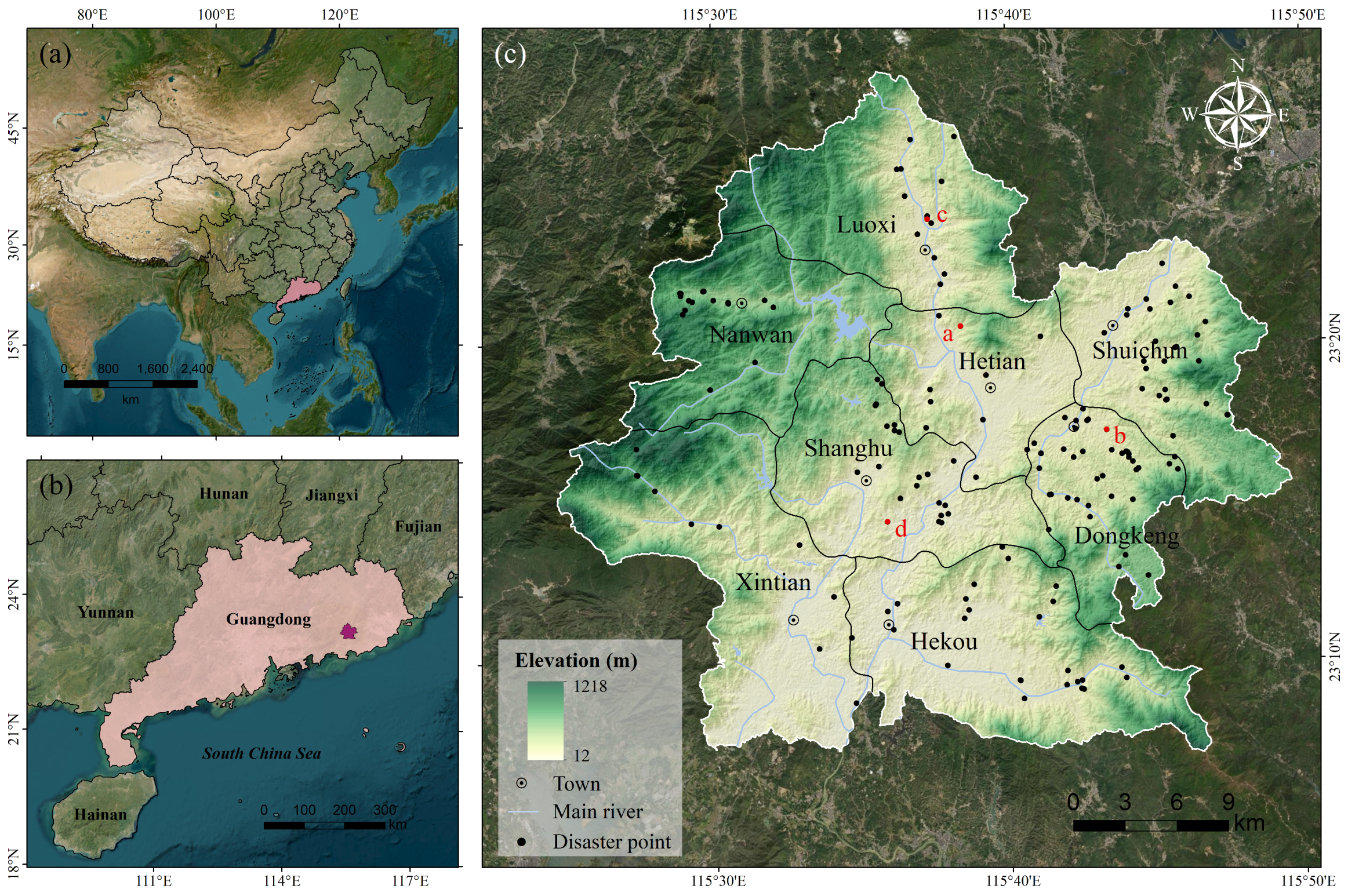
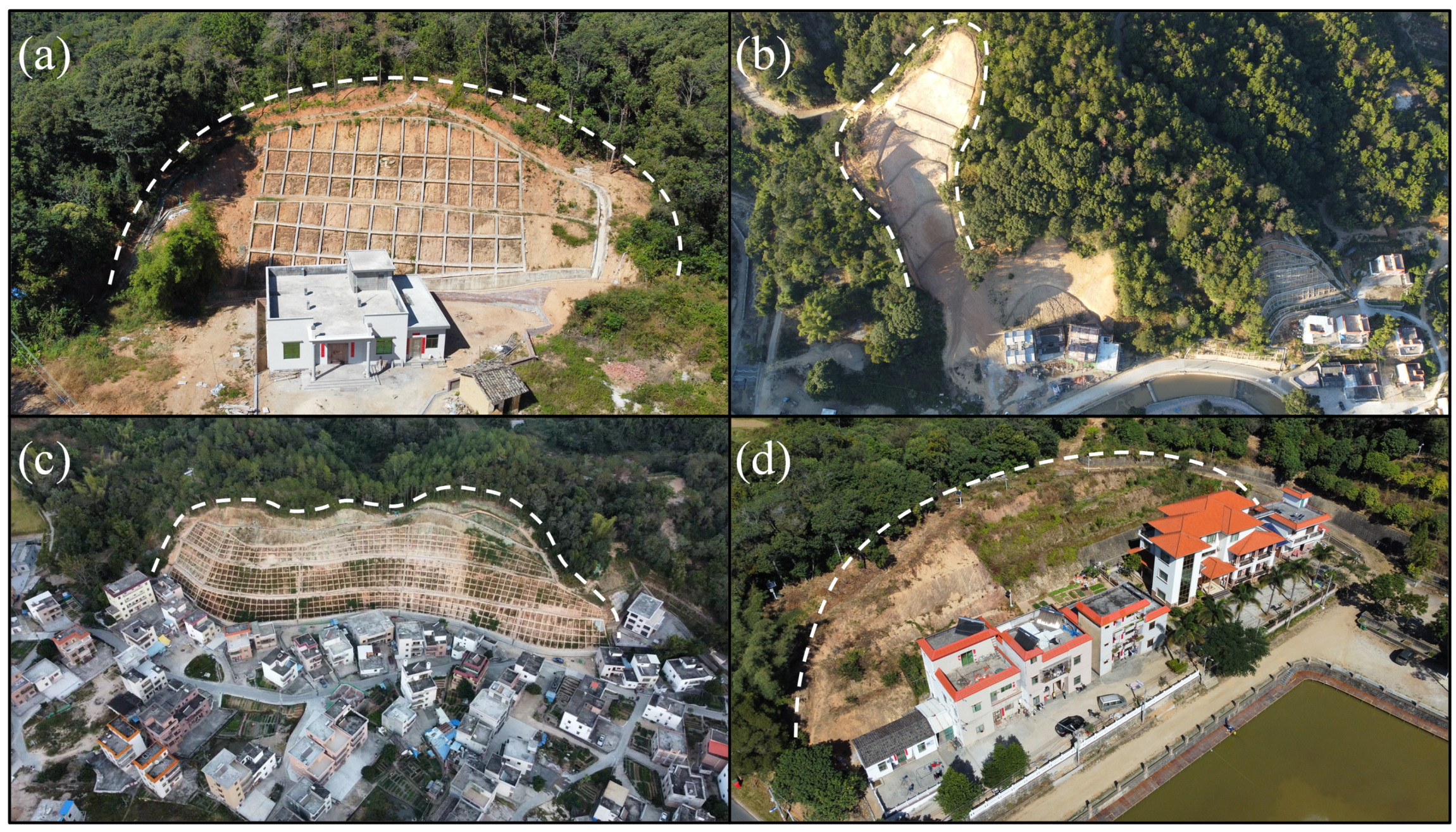
2.1. Study Area

The study area, Luhe County, covers 986 km2 on the southeastern coast of Guangdong Province, located between 115°24′ to 115°49′ E and 23°08′ to 23°28′ N (Figure 1). The topography is characterized by higher elevations in the east and west, with a lower central region. The central and southern areas consist of river terraces and alluvial plains, while the northwestern and southeastern areas are dominated by medium-low mountains. The elevation in the study area ranges from 12 to 1219 m, with mountainous areas above 500 m covering 263.6 km2. Luhe County is situated in a subtropical monsoon climate zone, with abundant rainfall. The average annual precipitation ranges from 1800 to 2400 mm, with the maximum annual rainfall reaching up to 3728 mm. The lithology of the study area can be classified into five types: single-layer soil, double-layer soil, multi-layer soil, layered clastic rock, and massive intrusive rock. The Lianhua Mountain fault runs through the central region, with gentle slopes and a large scale. The river system is mainly formed by tributaries of the Luo and Rong rivers, with significant elevation drops in the riverbeds, providing abundant hydropower resources. Combined with active human engineering activities, these features lead to frequent landslides, posing a serious threat to public safety.

2.2. Data Source

Digital Elevation Model (DEM) data were used to process landslide driving factors, including slope. The land use data, covering ten major types—such as arable land, woodland, grassland, shrubland, wetland, water bodies, tundra, artificial surfaces, bare land, and glaciers—were sourced from GlobeLand30 (http://loess.geodata.cn). Upon comparison, the 2020 land use data for Luhe was found to closely resemble that of 2000, thus addressing concerns regarding data timeliness in relation to the landslide occurrence period [36]. Therefore, the 2020 land use data was chosen for its higher quality and closer alignment with the landslide survey timeline. Additionally, vector data for roads, rivers, and faults were used for distance-based analysis. A summary of the dataset characteristics is provided in Table 1.
The landslide inventory used in this study was primarily obtained from historical landslide records registered by the Luhe County Bureau of Natural Resources. These landslides were documented through field measurements and on-site investigations conducted by local government authorities. The inventory includes detailed information such as landslide names, affected areas, hazard scales, deformation and failure characteristics, disaster features, and their developmental trends. Additionally, the most recent geological hazard risk survey in Luhe County was leveraged to further supplement and verify the landslide data. This effort involved 1:10,000 remote sensing interpretation across a 986 km2 area, with disaster and hazard points systematically reviewed. Field engineering investigations were also conducted using administrative villages as the basic spatial unit, resulting in over 80% of the landslide points being verified on-site. Ultimately, a total of 166 landslides were confirmed. Among these, 124 were classified as small-scale landslides (<10 × 104 m3), while 42 were medium-scale (10 × 104–100 × 104 m3). The majority of the identified landslides are soil-type, with gravel landslides being less common. Based on lithological characteristics, landslides were categorized into accumulation landslides and clay landslides. Accumulation landslides mainly consist of quaternary deposits or anthropogenic accumulations such as gravel and slag, while clay landslides are primarily composed of clayey soils with gravels, silty clay mixed with pebbles, and fragmented rock. In terms of morphology, the landslides generally exhibit tongue-shaped planar features and concave longitudinal profiles. Spatially, they are predominantly concentrated in the low mountainous and hilly areas of Nanwan, Shanghu, Dongkeng, and Shuichun towns. Figure 2 illustrates examples of four representative landslides in Luhe County, as marked in Figure 1c. These images were captured by UAV during field verification.

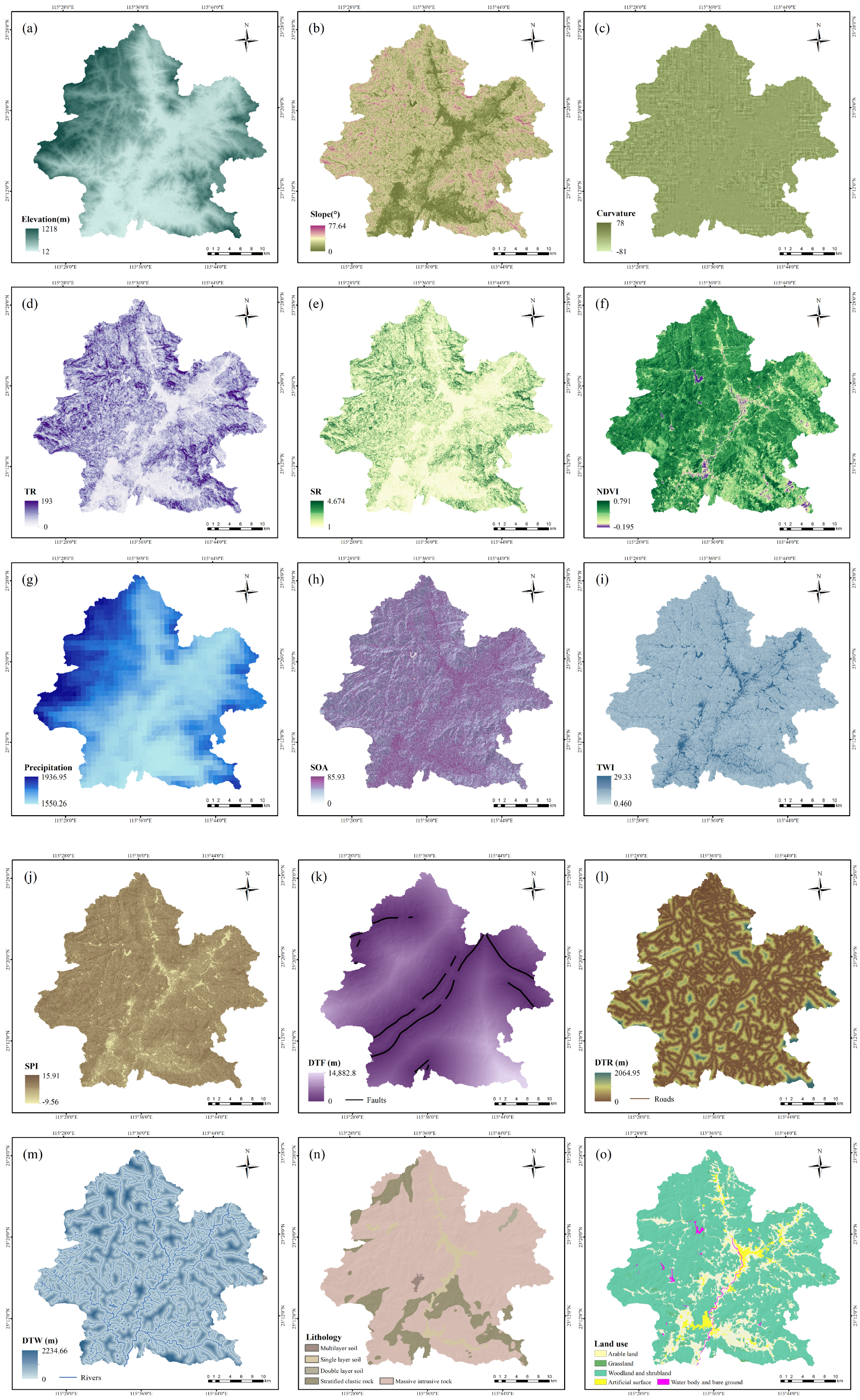
2.3. Landslide Conditioning Factors

Landslide occurrence is influenced by both natural and human factors. Precipitation, particularly intense short-term rainfall is often considered a triggering factor due to its immediate impact on landslide stability. Such studies typically involve collecting accurate precipitation amounts before and after landslide events, as well as determining the number of landslides triggered by precipitation [37,38]. In this study, we utilized the average annual precipitation data from 2003 to 2022 (with a resolution of 1000 m). The average annual precipitation accounts for the lag effect of precipitation on landslides, as it may not immediately trigger a landslide. Instead, landslides are more likely to occur after prolonged water infiltration, when the soil saturation reaches a critical level. As a result, average annual precipitation was included as one of the environmental factors to better capture its spatial variability in influencing landslide occurrences, in conjunction with other factors. Ultimately, considering the geological and environmental characteristics of the study area, 15 LCFs were preliminarily selected, including geological, topographical, hydrological, and human activity factors: elevation, slope, curvature, terrain relief (TR), surface roughness (SR), normalized difference vegetation index (NDVI), precipitation, slope of aspect (SOA), terrain wetness index (TWI), stream power index (SPI), distance to fault (DTF), distance to road (DTR), distance to water (DTW), lithology, and land use.
Considering the study area coverage and the computational complexity of the model, all raster layers were standardized to a spatial resolution of 30 m × 30 m. Data processing and visualization were performed using ERSI ArcGIS 10.8 and ENVI 5.6 software. The thematic layers of various LCFs are shown in Figure 3.

3. Methodology

Figure 4 illustrates the main workflow of this study: (1) collecting the landslide inventory of Luhe County and initially selecting 15 landslide conditioning factors to construct a GIS dataset; (2) applying GeoDetector to perform factor selection based on optimal reclassification; (3) inputting the selected factors into RF and GWRF models to construct the GeoD-RF and GeoD-GWRF models; (4) comparing and evaluating the performance of these hybrid optimized models; and (5) exploring the spatial relationships between LCFs and landslides.

3.1. Preparation of the Sample Set

For large-scale study areas with limited landslide inventories, it is common to represent each landslide by its centroid, a method shown to be effective in previous work [39,40]. In supervised machine-learning models, sample preparation is indispensable: non-landslide (negative) samples are as critical as landslide (positive) samples in regional susceptibility mapping. Previous studies typically define buffer zones at a fixed distance around known landslide sites and then randomly select negative samples from outside these buffers [41,42]. The selection of non-landslide samples by this method is highly subjective and random, reflecting only that no landslides have occurred at these locations to date; however, because potential landslides continually evolve, these points may still experience failure in the future [43]. Other studies have opted to draw negative samples from specific areas (such as zones of low slope), but this strategy concentrates negatives in geologically homogeneous regions, thereby overlooking other influential factors associated with landslides and potentially biasing model performance [44]. To improve the quality of negative–sample selection, Hu et al. (2020) [45] developed a fractal-theory–based method targeting very-low susceptibility areas, which outperformed traditional sampling from low-slope and landslide-free zones. Khabiri et al. (2023) [44] introduced the PISA-m classification framework, integrating geotechnical parameters into the sampling process and cautioning that conventional non-landslide–zone sampling can induce model overfitting. In their recent work, Dou et al. (2023) [46] applied an information-value model to partition susceptibility zones and demonstrated that drawing negative samples from low and very-low susceptibility regions substantially enhances model performance.
The various methods for selecting non-landslide samples described above have been demonstrated effective. Considering the study area’s characteristics as well as the completeness and quality of collected data, we decided to employ the information value model to determine landslide negative samples. Based on probability theory, the information value model is a commonly used statistical method in landslide susceptibility mapping, assigning a weight to each categorical unit and using the resulting entropy value to represent the probability of geological disasters; the larger the information value, the greater the likelihood of landslide occurrence within that unit. By characterizing factor influence through entropy magnitude, this approach offers a simple and effective means of representing the combined contribution of multiple factors to landslide susceptibility. Selecting negative samples from regions with low information values improves the precision of chosen samples and avoids dominance by any single influencing factor. The fundamental formula of the information value model is as follows:
I V i = ln N i / N S i / S
I V = i = 1 n I V i = i = 1 n ln N i / N S i / S
where S represents the total area of the study region, and N denotes the total number of landslides. Si and Ni refer to the area and the number of landslides within the i-th interval of a given factor, respectively. IVi is the information value of the i-th interval, while IV represents the total information value for the entire study area.

3.2. GeoDetector

GeoDetector is a spatial-based multivariate statistical model used for quantitatively evaluating the impact of a potential factor on a spatial phenomenon [47]. It makes minimal assumptions about the data, potentially overcoming the limitations of other statistical methods when dealing with spatial variables and providing clear physical interpretations [48]. The core assumption of GeoDetector in landslide studies is that if LCFs control or contribute to landslide occurrences, the spatial distribution of landslides should resemble the spatial distribution of these conditioning factors. Therefore, GeoDetector can reveal the underlying driving forces of a phenomenon by quantifying the influence of individual factors, making it suitable for factor selection. The factor detector within GeoDetector is used to assess the spatial heterogeneity of landslides (y) and evaluate the explanatory power of a LCF (x) on this spatial heterogeneity. By performing overlay analysis on the y-layer and x-layer, local and global variances are calculated to detect whether the x-layer contributes to the spatial distribution of landslides (Figure 5b). If x and y are correlated, a similar spatial pattern will exist between the two (Figure 5c). The explanatory power is ultimately measured by the q-value, calculated as follows:
q = 1 1 N σ 2 n = 1 Z N n σ n 2 = 1 W S S T S S
W S S = n = 1 Z N n σ n 2
T S S = N σ 2
where Z represents the number of zones in the x-layer, while N n and N denote the sample sizes in zone n and the entire study area, respectively. σ n 2 and σ 2 correspond to the variance of the dependent variable in zone n and the entire study area. WSS is the sum of within-zone variances, and TSS is the total variance of the entire area. The range of the q is [0, 1], where a higher q value indicates a stronger explanatory power of the independent variable X on the spatial heterogeneity of the dependent variable Y, and vice versa. The GeoDetector analysis was implemented using the GD package (version 10.3) in R.

3.3. Random Forest Model

The random forest (RF) is an ensemble machine learning method proposed by Breiman (2001) [49]. It combines multiple Decision Trees (DTs) through a random sampling approach for classification and regression tasks. The working principles of RF, as illustrated in Figure 6c, can be summarized as follows: (1) A bootstrap sampling is performed on the original training dataset to randomly select n new sample subsets with replacement; (2) select a set of features randomly at each re-sampling, and build n decision trees on this basis; (3) The generated trees are then aggregated to form a random forest, where the final output is determined by combining the predictions of each DT. Each sample subset used to create a DT represents two-thirds of the total samples, while the remaining samples are referred to as the out-of-bag (OOB) set. By calculating the OOB error, the relative importance of the LCFs in the prediction results can be quantified. The formula for calculating LCF importance is as follows:
L C F i x = 1 n t O O B M S E ,   p e r m x t O O B M S E t
where L C F i x represents the importance of the landslide conditioning factor x, n is the total number of trees in the forest, O O B M S E t is the mean square error of tree t before x is permuted, and O O B M S E ,   p e r m x t is the mean square error of tree t after x is permuted.
RF mitigates the tendency of a single DT to overfit and exhibits high tolerance to outliers and noise [50]. Due to its robustness and accuracy in handling complex data, the RF model has been widely applied in LSM, showing promising performance [12,17]. The RF model of this study was implemented using the randomForest package (version 4.7-1.1) in R.

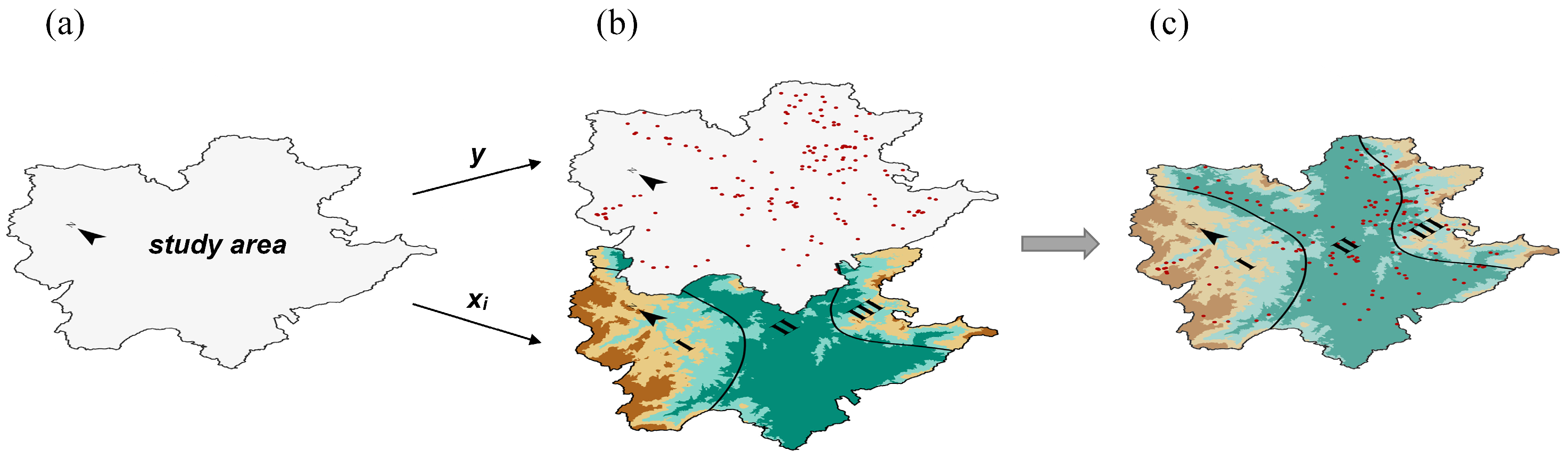
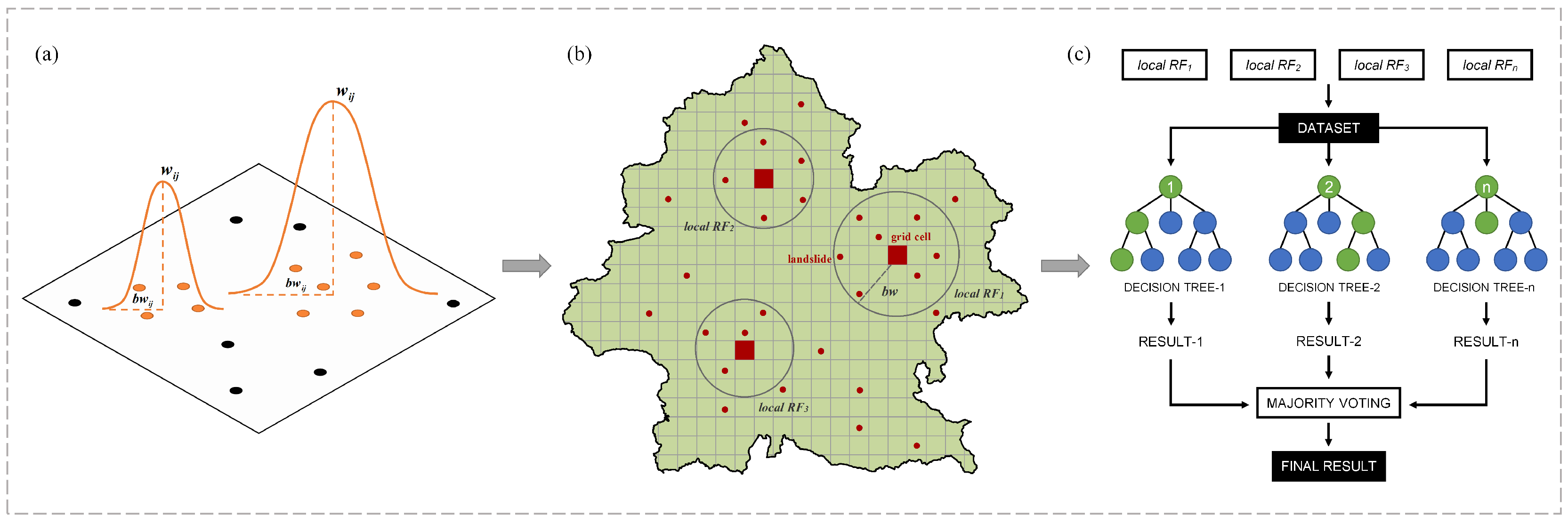
3.4. Geographical Weighted Random Forest Model

Although RF shows high applicability in LSM, it remains a global model. The global model is based on the assumption that the relationship between factors and landslides is constant across the entire spatial domain, thereby overlooking the spatial non-stationarity of the variables. Geographical Weighted Random Forest (GWRF) model extends RF by incorporating spatial dependencies, allowing for the consideration of the spatial heterogeneity of the variables themselves [51]. The working principles of GWRF are similar to geographically weighted regression. Specifically, the GWRF model incorporates the spatial location information of variables into the RF model. By fitting variable datasets located at different spatial positions, it generates local RF sub-models for each spatial unit (Figure 6). Thus, the simplified equation for the GWRF model can be expressed as:
Y i μ i , ν i = f x i , μ i , ν i + ε i
where f x i , μ i , ν i represents the prediction of the local RF calibrated based on position i, and μ i , ν i is the coordinate of the spatial unit at location i.
Each local RF sub-model covers a spatial range of data known as its neighborhood, and the parameter controlling the size of the neighborhood is called bandwidth (Figure 6a). There are two types of bandwidth: adaptive and fixed. The adaptive bandwidth ensures that the number of samples in each neighborhood is consistent, while the fixed bandwidth generates neighborhoods of uniform spatial range. In this study, the adaptive bandwidth GWRF model was adopted because it allows the neighborhood size to vary, making it more flexible for landslide data with different spatial sampling densities [52]. The GWRF model of this study was implemented using the SpatialML package (version 0.1.7) in R.

3.5. Validation of Models

For landslides, a typical binary classification problem, the receiver operating characteristic (ROC) curve is an effective tool to evaluate the predictive ability of a model [53]. The ROC curve, derived from the confusion matrix, reflects the dynamic changes in classification results. The accuracy of the ROC curve is interpreted by calculating the area under the curve (AUC). The AUC ranges from [0.5, 1], with higher AUC values indicating better model performance [54]. The relevant formulas derived from the confusion matrix are as follows:
S e n s i t i v i t y = T P T P + F N
S p e c i f i c i t y = T N F P + T N
A U C = T P + T N P + N
where TP (true positive) represents the number of correctly classified landslide samples, TN (true negative) represents the number of correctly classified non-landslide samples, FP (false positive) represents the number of landslide samples incorrectly classified, and FN (false negative) represents the number of non-landslide samples incorrectly classified. P and N denote the total number of positive and negative samples, respectively.

4. Result

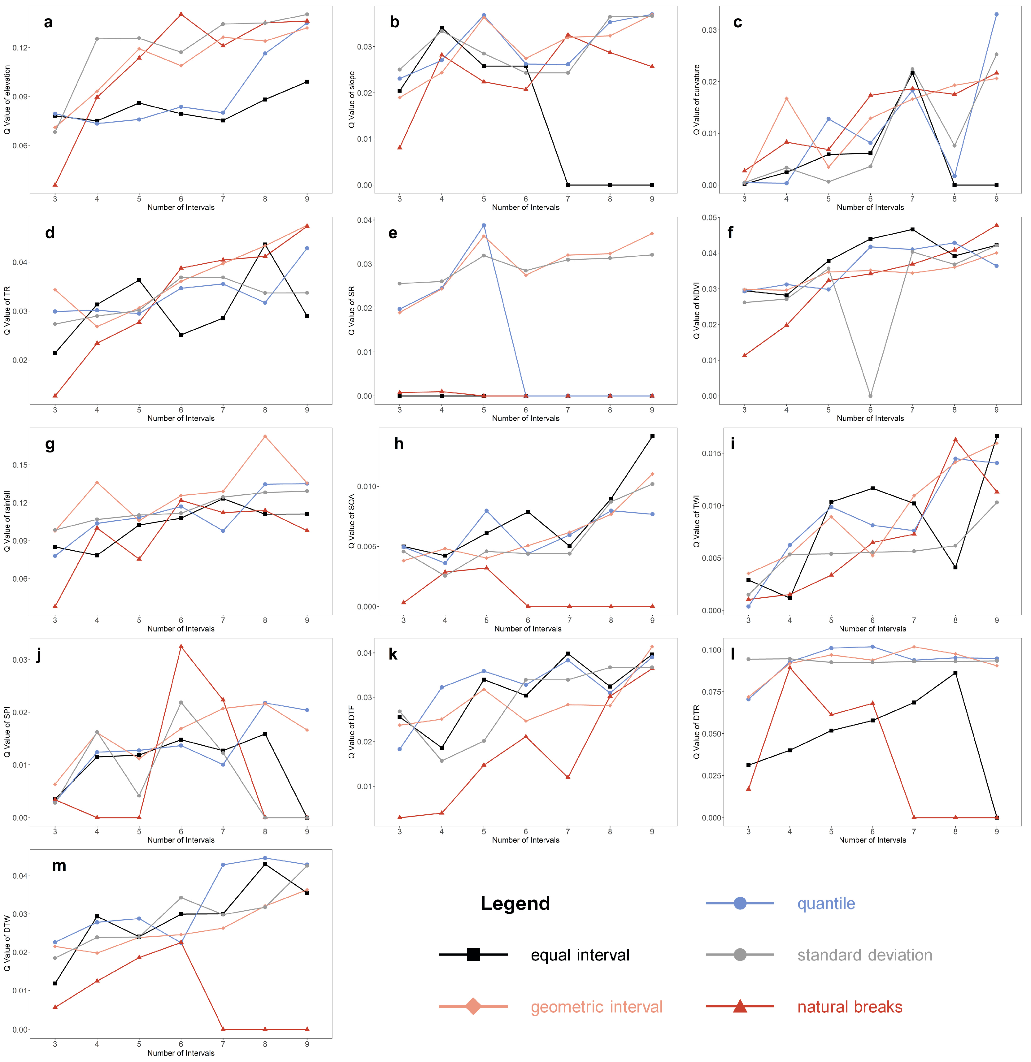
4.1. Exploration and Selection of Landslide Conditioning Factors

GeoDetector can handle both numerical variables (e.g., slope, elevation, NDVI) and qualitative variables (e.g., lithology, land use). However, for continuous data, reclassification is necessary before applying GeoDetector to enhance spatial analysis [55]. Previous studies employing GeoDetector for LCFs selection typically used manual or natural breaks methods to categorize continuous variables, with no standardized approach for determining the number of classification intervals [18,25]. However, for a spatial statistical model like factor GeoDetector, the classification of variables can significantly influence the calculation of the explanatory power, represented by the q value. In this study, five methods: equal interval, natural breaks, quantile, geometric interval, and standard deviation, were employed to determine the optimal reclassification scheme for each continuous variable. Considering the data volume and computational complexity, the classification number range for all methods was set to the commonly used [3, 9]. The highest q value for each factor across different classification methods and numbers of intervals was identified as the factor’s optimal explanatory power for landslides. The variation in q values for each LCF under different reclassification schemes is shown in Figure 7. For example, for elevation, the best explanation of its influence on landslides is achieved when it is classified into six classes using the natural breaks method.
Ultimately, GeoDetector was applied based on the optimal reclassification scheme for each factor, and the factor detection results for all LCFs are shown in Figure 8. It can be observed that precipitation and elevation have the strongest potential influence on landslides in the study area, which is consistent with our previous findings using the GWR model to investigate landslide driving factors in Luhe [56]. According to statistics, the average elevation of 166 landslide points is only 200.87 m, often located in low-altitude areas with frequent human activity. As elevation decreases, the intensity of road construction and land development increases. The q values of DTR and land use rank third and fourth, respectively, which not only validates the reasonableness of the GeoDetector results but also highlights that, in addition to precipitation, anthropogenic factors are a significant cause of landslides in the study area.
The p values corresponding to the q values of the LCFs indicate the significance of each influencing factor, with the confidence interval for the significance test set at 95%. As observed, the factors curvature, SPI, TWI, and SOA did not pass the significance test, and their q values are relatively low. This suggests that these four factors have a weaker explanatory power for landslide spatial distribution. As a result, we excluded these four factors and selected the remaining 11 factors: elevation, slope, terrain relief, surface roughness, normalized difference vegetation index, precipitation, distance to fault, distance to road, distance to water, lithology, and land use, as the main factors for further analysis in subsequent models.

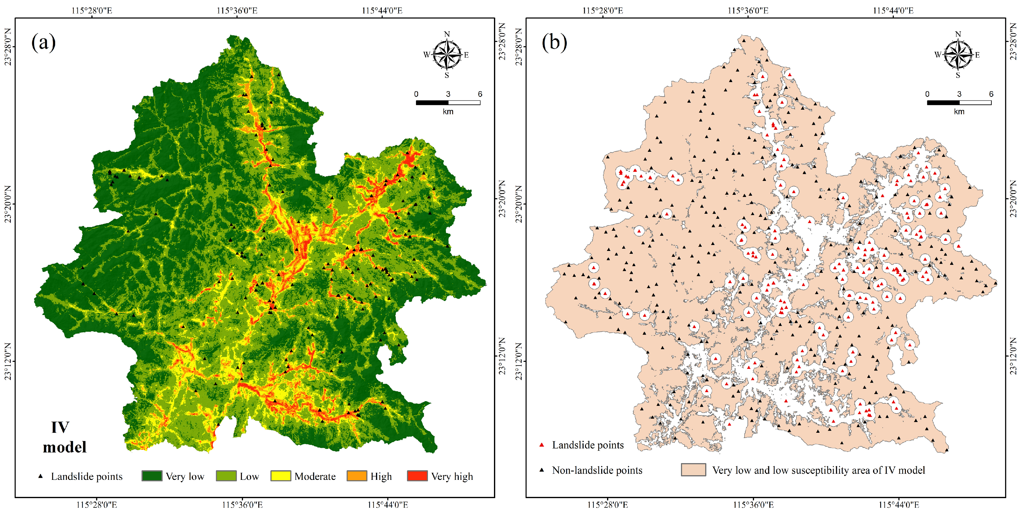
4.2. Generation of Non-Landslide Samples Based on the Information Value Model

The selected landslide conditioning factors were analyzed using GIS, with continuous variables classified using the natural breaks method. For each factor, the number of landslides and the area within each classified interval were extracted. The factors DTF, DTR, and DTW were classified based on empirically determined influence ranges. Subsequently, the proportions of landslide occurrences and area coverage were calculated for each interval. For intervals containing no landslide points, an average information value was considered, and an information value of –2 was directly assigned. The resulting information values for each factor, calculated using Equation (1), are presented in Table 2.
Using the raster calculator in GIS, the factor layers were overlaid based on Equation (2) to generate a preliminary landslide susceptibility map for Luhe County. This map was then classified into five susceptibility levels using the natural breaks method (Figure 9a). Very low and low susceptibility zones identified by the information value model were designated as non-landslide areas. Within these zones, a number of non-landslide points equal to twice the number of landslide samples were randomly generated. Additionally, it was ensured that all non-landslide points were located at least 500 m away from any positive sample (Figure 9b). This strategy aims to (1) prevent the LCFs attributes of non-landslide samples from being too similar to those of positive samples or to one another, which could otherwise affect model training, and (2) increase the number of negative samples—while maintaining their reliability—to reduce the risk of overfitting when the overall sample size is limited. Ultimately, 70% of all samples were used for model training, while the remaining 30% were reserved for validation.

4.3. Model Implementation and Performance Evaluation

In order to investigate the impact of GeoDetector factor selection on the model and compare the performance differences between local and global machine learning models, four models were constructed: RF, GeoD-RF, GWRF, and GeoD-GWRF. The initial factors and the selected factors were used as inputs for these models, respectively. To avoid overfitting in the GWRF model, grid search was employed to determine the optimal combination of hyperparameters. For each step size, 5-fold cross-validation was used to mitigate the risk of random variations in the parameters. The final hyperparameter settings for GWRF were as follows: adaptive kernel, bandwidth = 80, ntree = 500, mtry = 4. For uniform comparison, the ntree and mtry parameters for the RF model were kept consistent.
The landslide susceptibility evaluation was conducted using the test dataset for the study area, and the prediction results were compared with the landslide validation dataset. The ROC curves and corresponding AUC values for different models are shown in Figure 10. As can be seen, the performance of the local machine learning model (GWRF), which considers spatial structure, is significantly better than that of the global machine learning model (RF). The AUC value increased from 0.915 to 0.937, a 2.41% improvement. This indicates that GWRF, by considering the spatial heterogeneity of the LCFs, better captured the nonlinear relationship between LCFs and landslides at the regional scale, taking into account the local importance of LCFs. Furthermore, after factor selection using GeoDetector, although the number of factors decreased from 15 to 11, the model performance did not deteriorate. On the contrary, both GeoD-RF and GeoD-GWRF were able to achieve better prediction results with a reduced number of factors. This demonstrates that the factor optimization by GeoDetector is reliable. It not only helps eliminate unimportant redundant data, thereby reducing the burden on the model, but also further enhances the accuracy of the model’s predictions.
In addition, we conducted a spatial autocorrelation test on the squared residuals of the predictions made by the four models, using Moran’s I as the test metric (Table 3). The range of Moran’s I is between −1 and 1. A positive value indicates spatial clustering of the elements, a negative value indicates spatial dispersion, and values close to 0 suggest spatial randomness [57]. As shown, all four models exhibited a slight spatial clustering effect in their prediction residuals. However, compared to RF, the GWRF model had a smaller Moran’s I value, indicating that its residuals were more spatially random. This suggests that the local decomposition method, which accounts for the spatial non-stationarity, is less affected by the spatial heterogeneity of the factors themselves and is therefore suitable for broader study areas. It is worth emphasizing that after factor optimization using GeoDetector, the Moran’s I values further decreased, with GeoD-GWRF achieving the smallest Moran’s I value of 0.106. This indicates that, after optimization by GeoDetector, the impact of LCFs’ spatial heterogeneity on the prediction results was further reduced. The factors excluded by GeoDetector were those with weaker spatial effects on landslides. These factors exerted a smaller driving influence on landslides, and their inclusion would have increased the model’s prediction uncertainty across the entire study area. This further validates the applicability and rationality of the GeoDetector.

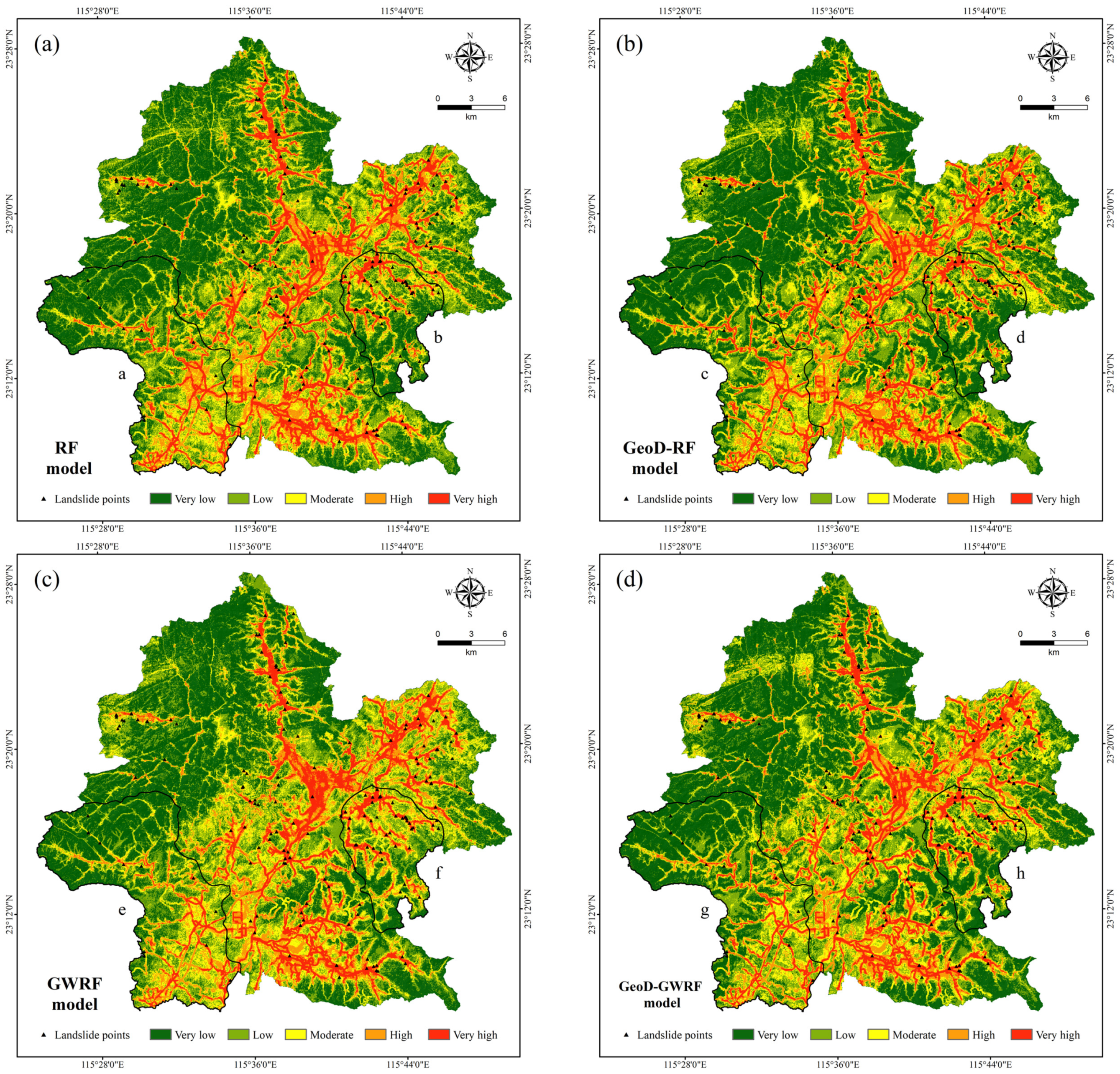
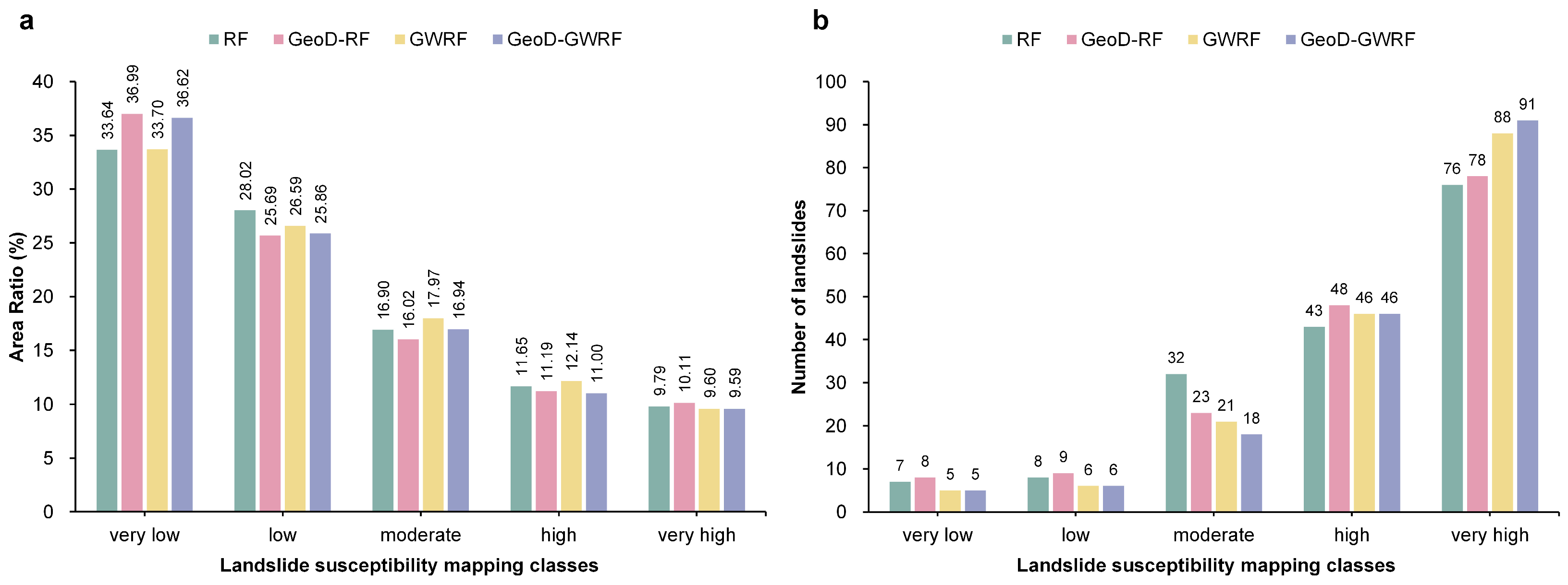
4.4. Differences in Landslide Susceptibility Mapping Across Models

The dataset for all grid cells was input into the four trained models to obtain landslide susceptibility evaluation results for the entire study area. The commonly used natural breaks method [24,58] was applied to classify each susceptibility layer into five susceptibility zones: very low, low, moderate, high, and very high. Finally, the landslide susceptibility maps for the four models are shown in Figure 11. By overlaying the landslide distribution map of the study area, it can be observed that the high and very high susceptibility zones from the four models are strongly correlated with the distribution of landslides.
Further statistical analysis of the results for each zone in relation to the landslide distribution (Figure 12) reveals that the area proportion of each zone decreases gradually from very low to very high susceptibility. However, the number of landslides in each zone increases progressively. This confirms the validity of the predictions made by the four models. The areas classified as very low susceptibility zones are larger in the GeoD-RF and GeoD-GWRF models (36.99% and 36.62%, respectively), while the RF model only classifies 33.64% of the area as very low susceptibility. At the same time, the very high susceptibility zones defined by GWRF and GeoD-GWRF are smaller (9.60% and 9.59%, respectively), but they predict more landslides in these zones (88 and 91, respectively). The local machine learning methods classify more areas into low susceptibility zones and fewer areas into high susceptibility zones, yet they yield more accurate prediction results. This is because local learning models account for the varying influence of factors in different regions, overcoming the limitation of global models, where factor importance is assumed to be constant across space. This makes the classification results more targeted. It is noteworthy that, compared to RF and GWRF, the GeoD-RF and GeoD-GWRF models, after factor optimization, predict more landslides with less area classified as very high susceptibility. Although the GeoD-GWRF model uses the fewest LCFs, it produces the most accurate zonal results. This indicates that the inclusion of redundant factors can actually reduce model performance, and the use of the GeoDetector method to exclude irrelevant LCFs is therefore justified.

5. Discussion

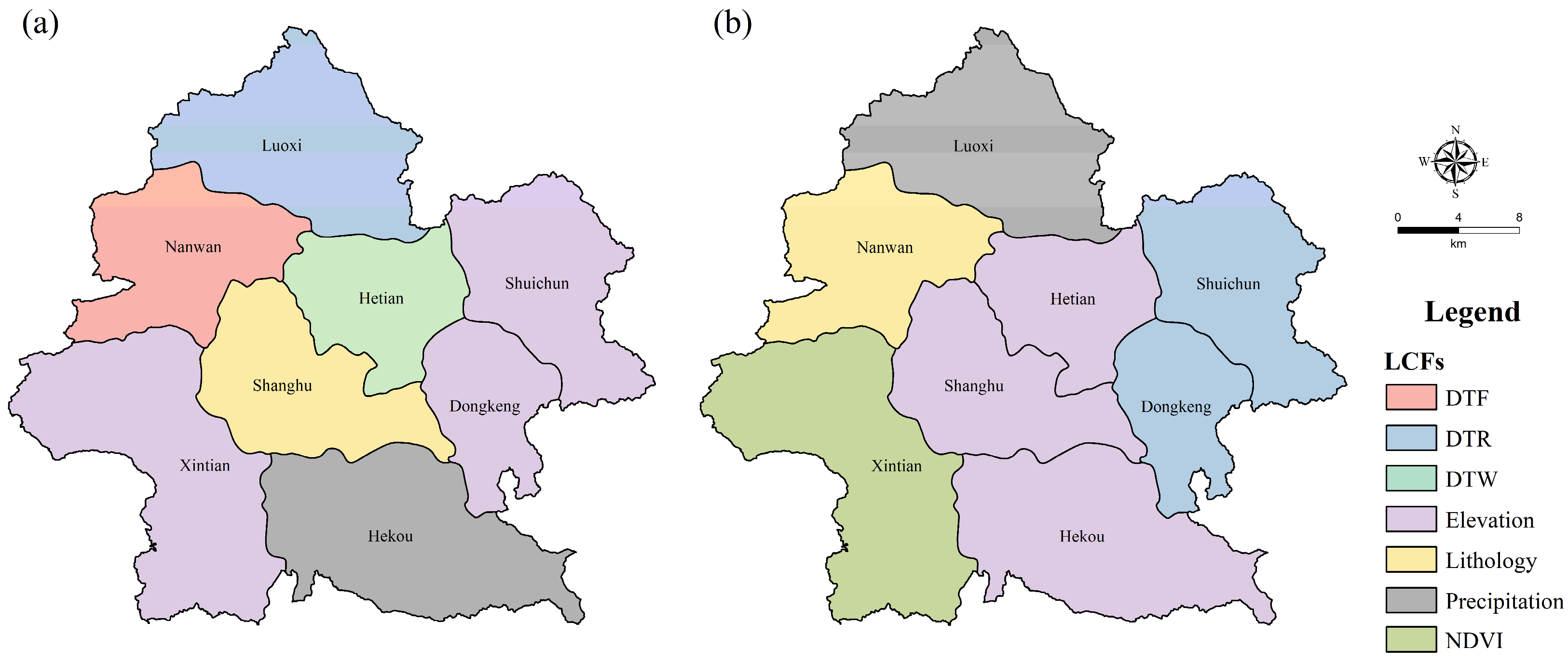
5.1. Local Interpretability of the GWRF Model

As a local decomposition of the RF model, the GWRF model’s results can be mapped individually, making it a useful exploratory tool [51]. Similar to the RF model, GWRF can also calculate the relative importance of factors to landslides by computing the OOB mean square error (Equation (6)). However, this importance is not spatially constant; instead, for each local model decomposition (corresponding to each sample point), there is a relative importance value. Specifically, the GWRF model allows factors to have different influence weights on landslides at different spatial locations, making the spatial influence of factors on landslides interpretable.
We averaged the LCFs’ importance calculated by all local models and used this as the global importance of LCFs computed by GWRF, which was then compared with the RF model (Figure 13a). It should be noted that the comparison here is based on GeoD-RF and GeoD-GWRF models, which were optimized by GeoDetector. At the global scale, the two models show little difference in the factors they consider most strongly correlated with landslides. Both models identify distance to roads, elevation, distance to water, terrain relief, and precipitation as the most important factors. However, the GWRF model regards distance to faults as more strongly correlated with landslides than NDVI. This may be because the NDVI is generally high in Luhe (Figure 3f), and the characteristics of NDVI in most of the divided local areas are similar, which weakens its influence. It is worth discussing that GeoDetector assesses the driving effect of factors on landslides by examining the spatial distribution of factors and their similarity to the spatial pattern of landslides across the entire study area, based on the spatial heterogeneity of the factors themselves. GWRF, on the other hand, decomposes the study area through bandwidths and calculates the relative importance by performing random forest simulations on each bandwidth. While this approach also takes into account the spatial heterogeneity of factors to some extent, the results inevitably differ from those obtained by GeoDetector. Interestingly, however, the results from RF and GWRF still show a high degree of similarity with the factor detection results from GeoDetector (Figure 8). All three methods identify elevation, precipitation, and distance to roads as having a significant impact on landslides.
Although the factor importance results from GWRF and RF are generally similar, there are differences in the factor importance results obtained by each local model within the GWRF framework. The characteristic of local weight reallocation in GWRF also leads to spatial differences in the susceptibility mapping results. To better illustrate the differences between local and global model predictions, we further extracted the susceptibility prediction results of the four models in Xintian, located in the southwestern part with fewer disaster points, and Dongkeng, in the eastern part with more disaster points (Figure 14). Additionally, we calculated the factor importance derived from GWRF in these two regions (Figure 13b).
As shown, in Xintian, which has fewer disaster points, RF and Geo-RF still predict a larger portion of the area as high susceptibility zones (Figure 14a,c). In contrast, GWRF and Geo-GWRF predict most of Xintian as low susceptibility zones (Figure 14e,g). As a global model, RF still considers DTR and elevation to be the main factors influencing landslides in Xintian (Figure 13a). However, GWRF identifies elevation and NDVI as the primary factors affecting landslides in this region (Figure 13b). The change in factor importance leads to differences in the landslide susceptibility predictions between the two models for this region. Although both models accurately predict all the landslides in Xintian, the GWRF model predicts a smaller area for high susceptibility zones. In other words, the GWRF prediction is more targeted because it identifies the most important factors influencing landslides in this region. For Dongkeng, which has more disaster points, GWRF identifies the five most important factors influencing landslides as DTW, elevation, DTR, TR, and precipitation (Figure 13b), while RF still considers DTR, elevation, TR, precipitation, and DTW to be the most important factors in sequence (Figure 13a). Since the most important factors remain largely unchanged, the prediction results from both models are quite similar, and each model makes correct predictions (Figure 14d,h). However, the GWRF model assigns higher weight proportions to DTW in this region, which leads to more areas near rivers being classified as high susceptibility zones. In summary, the local learning characteristics of the GWRF model enable it to better capture the impact of LCFs’ spatial heterogeneity on landslides. By considering the differences in the importance of the same factor across different regions, it makes more targeted judgments on the final landslide susceptibility predictions. This not only improves the accuracy of the predictions but also helps reduce the associated costs of disaster prevention and mitigation efforts.
Based on the local interpretability of the GWRF model, we compiled the results from all local models within each town and identified the two most influential factors affecting landslides in each area (Figure 15). It can be observed that elevation and distance to roads play significant roles in multiple towns. In Dongkeng and Shuichun—areas severely affected by landslides—distance to roads ranked as the second most important factor, indicating that elevation-driven human activities, especially road construction, have a strong impact on landslide occurrence in these regions. In Hetian, river-induced slope disturbances emerged as the primary trigger for landslides. Meanwhile, in Nanwan and Shanghu, the dominant influencing factors were distance to faults and lithology, respectively, suggesting that greater attention should be paid to fault activity and lithological variation in these areas when assessing landslide risk.
To better account for the spatial heterogeneity of landslide conditioning factors, we further examined the influence of each factor across different geomorphic types. The geomorphic classification was based on the macro-geomorphological system of China proposed by Chenghu et al. (2009) [59], which utilizes the terrain relief index to divide landforms into five types: plain, platform, hill, low relief mountain, middle relief mountain, high relief mountain, and highest relief mountain. Referring to the latest “China land 1:1 million digital geomorphic classification system” [60,61] and considering the scale of the study area, we simplified the classification into four geomorphic types: plain (<10 m), platform (10–30 m), hilly (30–50 m), and low mountain (>50 m) (Figure 16a). We then identified the dominant LCF within each geomorphic type (Figure 16b). The plain areas are primarily located in the low-elevation zones of the study area, where elevation emerged as the most important influencing factor. Notably, the average elevation of all 166 landslide points was only 200.87 m, significantly lower than the study area’s mean elevation of 314 m. This indicates that landslides are more likely to occur in low-lying zones with intensive human activity, a trend consistent with findings from many studies in southeastern coastal China [7,62,63]. It suggests that anthropogenic factors—such as infrastructure development and land use change—may be the primary drivers of local hazards in these plain regions. In the platform and hilly areas, the dominant LCFs were distance to water and distance to road, respectively. This implies that in platform zones, increasing terrain variation enhances the erosive and scouring effects of water on slopes, making hydrological processes a major driver of landslides. In contrast, in hilly regions, road construction poses a greater disturbance to slope stability, indicating the need for proper road planning, as well as reinforcement of roadside slopes and drainage systems. Low mountain areas, characterized by high elevation and significant terrain variation, tend to facilitate the development of vertical joints. As elevation increases, gravitational potential energy acting on slopes also rises, making these areas more susceptible to landslides. Here, terrain relief was identified as the most critical factor influencing landslide occurrence. By visualizing the local importance of each factor in both township and geomorphic units, the GWRF model provides new insights that can guide region-specific disaster prevention and mitigation efforts.

5.2. Generalizability of the Proposed Method for Landslide Susceptibility Mapping

To enhance the accuracy of landslide susceptibility assessment, this study employed the p-value threshold from GeoDetector’s significance test to select the LCFs most strongly associated with landslide occurrences. The selected factors were then analyzed using the GWRF model, which incorporates local modeling to account for spatial heterogeneity. To evaluate the effectiveness of the proposed approach, we compared it with two widely used machine learning models: logistic regression [11] and support vector machine (SVM) [14]. Additionally, we applied multicollinearity testing as an alternative method for LCF selection, and compared its performance against GeoDetector-based selection when combined with the different models. Multicollinearity among variables was assessed using two common indicators: tolerance (TOL) and the variance inflation factor (VIF). When TOL < 0.2 and VIF > 5, multicollinearity is considered to be significant among the explanatory variables [37]. A high VIF indicates a strong correlation among factors, suggesting potential data redundancy. As shown in Table 4, the initial multicollinearity test revealed strong collinearity between elevation and precipitation, as well as between slope and surface roughness. Considering this, the surface roughness and precipitation factors were excluded. After removal, the remaining factors exhibited only weak correlations (VIF < 5), indicating acceptable levels of multicollinearity.
Subsequently, all factors, the factors selected through VIF, and the factors selected through GeoDetector were incorporated into each model. To examine potential overfitting issues, we applied a 5-fold cross-validation method, randomly dividing the sample set for five rounds of training and validation. The median and standard deviation of accuracy, AUC, recall, and F1 score for each model were calculated (Table 5), and ROC curves for each model were plotted (Figure 17). The results showed that the performance of each model across different data subsets was stable, with small standard deviations, indicating good generalization capability and a low risk of overfitting. After factor selection using VIF, both the accuracy and AUC values for the logistic regression model improved, and the model’s recall and F1 score were 0.580 and 0.611, respectively, surpassing the Geo-Logistic model. However, for the SVM, RF, and GWRF models, the performance metrics slightly declined. This suggests that while the VIF method helped reduce data redundancy and multicollinearity to some extent, it also removed some factors strongly related to landslides, leading to a decrease in model accuracy. Additionally, multicollinearity issues tend to affect linear regression models like logistic regression more significantly, while machine learning models are less influenced by correlations between variables and are more focused on the relationship between dependent and independent variables. For the SVM model, the AUC values were 0.843, 0.842, and 0.844 for the three factor sets, demonstrating that the SVM model showed good adaptability to different data and exhibited better generalization ability and stability. In contrast, the RF and GWRF models, based on binary tree splitting mechanisms, have higher data quality requirements, and the results varied considerably across different factor sets. After removing the rainfall factor, which had a strong influence on landslides, using VIF, the performance of both models significantly decreased. Overall, the dataset constructed using the factors selected by GeoDetector’s q and p threshold values effectively captured the spatial correlation between the dependent and independent variables. It removed less influential factors, reducing data size while enhancing the performance of the machine learning models. Based on comparisons of accuracy and AUC, the GWRF model consistently demonstrated superior performance. This local modeling approach accounts for geographic, topographic, and environmental factors in the region, making it more effective for predicting and modeling small spatial clusters, resulting in more accurate and targeted predictions.

5.3. Limitations of the Current Study

Although the Geo-GWRF model effectively removes redundant factors unrelated to landslides and addresses the linear limitations and inefficiency issues faced by traditional geographically weighted regression when dealing with large spatial datasets [64], there are still some limitations in this study that warrant further improvement in future work.
First, the criteria for factor selection using GeoDetector were somewhat limited. In this study, factors unrelated to landslides were removed based on a p-value threshold of 0.05. However, some studies have also achieved good results by directly defining q-values or combining other factor selection methods, such as information gain ratio [25,65]. The standard for factor removal when using GeoDetector for LSM has not yet been standardized, and the most optimal method still warrants further discussion in future research. Additionally, Luhe is located in a subtropical monsoon climate zone, and the consideration of factors such as seasonal precipitation is still part of the future work plan.
Secondly, there are still some limitations in the interpretability of the GWRF model itself. GWRF calculates the strength of factor importance by assessing error increments, but due to the “black-box” nature of machine learning, it cannot reveal the direction of the factor’s influence. In other words, we cannot determine whether an increase or decrease in a specific factor’s characteristics leads to a positive or negative effect on landslides. However, we have noticed that a machine learning interpretation method called SHapley Additive exPlanations (SHAP) has shown promising results [66,67]. We aim to combine this method with GWRF to better understand the impact of LCFs on landslides at the local scale.

6. Conclusions

This study proposes a new method that combines GeoDetector and GWRF local machine learning to fully account for the impact of spatial heterogeneity of landslide conditioning factors in landslide susceptibility prediction. The results show that the GeoD-GWRF model can effectively remove disaster-related factors that are not associated with landslides from a spatial differentiation perspective. Based on the results from the ROC curve and Moran’s I, the GeoD-GWRF model achieves higher prediction accuracy and is applicable to a broader study area. At the same time, the predictions from the local machine learning method are more targeted. By leveraging the local interpretability of GeoD-GWRF, related costs in disaster prevention and mitigation can be reduced, offering new perspectives for landslide prevention and control in different regions of the study area.

Author Contributions

Conceptualization, F.L. and G.Z.; Methodology, F.L. and G.Z.; Software, F.L., G.Z., T.W. and Y.Y.; Validation, F.L. and Q.Z.; Formal analysis, Y.Y. and Q.Z.; Resources, G.Z. and T.W.; Data curation, F.L., G.Z., T.W., Y.Y. and Q.Z.; Writing—original draft, F.L. and G.Z.; Writing—review and editing, F.L. and G.Z.; Visualization, F.L., G.Z., T.W. and Y.Y.; Supervision, Y.Y. and Q.Z.; Project administration, G.Z., T.W., Y.Y. and Q.Z.; Funding acquisition, G.Z. All authors have read and agreed to the published version of the manuscript.

Funding

This work was supported by the Guangdong Basic and Applied Basic Research Foundation (No. 2025A1515011669), the Guangdong Special Fund for National Park Construction (No. 2021GJGY026), and the Science and Technology Program of Guangzhou, China, under Grant (No. 201707010209).

Data Availability Statement

The original contributions presented in the study are included in the article, further inquiries can be directed to the corresponding author.

Acknowledgments

The authors would like to thank Junwei Zhen (Huizhou Geological Survey Center, Guangdong Provincial Bureau of Geology) for providing the original data used in this study. The authors are also grateful to the editor and the anonymous reviewers for their constructive comments and suggestions on the manuscript.

Conflicts of Interest

The authors declare no conflicts of interest.

References

  1. Han, Z.; Su, B.; Li, Y.; Ma, Y.; Wang, W.; Chen, G. Comprehensive analysis of landslide stability and related countermeasures: A case study of the Lanmuxi landslide in China. Sci. Rep. 2019, 9, 12407. [Google Scholar] [CrossRef]
  2. Petley, D. Global patterns of loss of life from landslides. Geology 2012, 40, 927–930. [Google Scholar] [CrossRef]
  3. Froude, M.J.; Petley, D.N. Global fatal landslide occurrence from 2004 to 2016. Nat. Hazards Earth Syst. Sci. 2018, 18, 2161–2181. [Google Scholar] [CrossRef]
  4. Huang, F.; Zhang, J.; Zhou, C.; Wang, Y.; Huang, J.; Zhu, L. A deep learning algorithm using a fully connected sparse autoencoder neural network for landslide susceptibility prediction. Landslides 2020, 17, 217–229. [Google Scholar] [CrossRef]
  5. Kaur, R.; Gupta, V.; Chaudhary, B. Landslide susceptibility mapping and sensitivity analysis using various machine learning models: A case study of Beas valley, Indian Himalaya. Bull. Eng. Geol. Environ. 2024, 83, 228. [Google Scholar] [CrossRef]
  6. Panchal, S.; Shrivastava, A.K. Landslide hazard assessment using analytic hierarchy process (AHP): A case study of National Highway 5 in India. Ain Shams Eng. J. 2022, 13, 101626. [Google Scholar] [CrossRef]
  7. Zhang, G.; Cai, Y.; Zheng, Z.; Zhen, J.; Liu, Y.; Huang, K. Integration of the statistical index method and the analytic hierarchy process technique for the assessment of landslide susceptibility in Huizhou, China. Catena 2016, 142, 233–244. [Google Scholar] [CrossRef]
  8. Zhang, W.; Liu, S.; Wang, L.; Samui, P.; Chwała, M.; He, Y. Landslide susceptibility research combining qualitative analysis and quantitative evaluation: A case study of Yunyang County in Chongqing, China. Forests 2022, 13, 1055. [Google Scholar] [CrossRef]
  9. Wang, Q.; Guo, Y.; Li, W.; He, J.; Wu, Z. Predictive modeling of landslide hazards in Wen County, northwestern China based on information value, weights-of-evidence, and certainty factor. Geomat. Nat. Hazards Risk 2019, 10, 820–835. [Google Scholar] [CrossRef]
  10. Aditian, A.; Kubota, T.; Shinohara, Y. Comparison of GIS-based landslide susceptibility models using frequency ratio, logistic regression, and artificial neural network in a tertiary region of Ambon, Indonesia. Geomorphology 2018, 318, 101–111. [Google Scholar] [CrossRef]
  11. Budimir, M.; Atkinson, P.; Lewis, H. A systematic review of landslide probability mapping using logistic regression. Landslides 2015, 12, 419–436. [Google Scholar] [CrossRef]
  12. Huang, F.; Cao, Z.; Guo, J.; Jiang, S.-H.; Li, S.; Guo, Z. Comparisons of heuristic, general statistical and machine learning models for landslide susceptibility prediction and mapping. Catena 2020, 191, 104580. [Google Scholar] [CrossRef]
  13. Yuan, R.; Chen, J. A novel method based on deep learning model for national-scale landslide hazard assessment. Landslides 2023, 20, 2379–2403. [Google Scholar] [CrossRef]
  14. Huang, Y.; Zhao, L. Review on landslide susceptibility mapping using support vector machines. Catena 2018, 165, 520–529. [Google Scholar] [CrossRef]
  15. Youssef, A.M.; Pourghasemi, H.R.; Pourtaghi, Z.S.; Al-Katheeri, M.M. Landslide susceptibility mapping using random forest, boosted regression tree, classification and regression tree, and general linear models and comparison of their performance at Wadi Tayyah Basin, Asir Region, Saudi Arabia. Landslides 2016, 13, 839–856. [Google Scholar] [CrossRef]
  16. Youssef, A.M.; Pourghasemi, H.R. Landslide susceptibility mapping using machine learning algorithms and comparison of their performance at Abha Basin, Asir Region, Saudi Arabia. Geosci. Front. 2021, 12, 639–655. [Google Scholar] [CrossRef]
  17. Sevgen, E.; Kocaman, S.; Nefeslioglu, H.A.; Gokceoglu, C. A Novel Performance Assessment Approach Using Photogrammetric Techniques for Landslide Susceptibility Mapping with Logistic Regression, ANN and Random Forest. Sensors 2019, 19, 3940. [Google Scholar] [CrossRef]
  18. Zhou, X.; Wen, H.; Zhang, Y.; Xu, J.; Zhang, W. Landslide susceptibility mapping using hybrid random forest with GeoDetector and RFE for factor optimization. Geosci. Front. 2021, 12, 101211. [Google Scholar] [CrossRef]
  19. Sun, D.; Shi, S.; Wen, H.; Xu, J.; Zhou, X.; Wu, J. A hybrid optimization method of factor screening predicated on GeoDetector and Random Forest for Landslide Susceptibility Mapping. Geomorphology 2021, 379, 107623. [Google Scholar] [CrossRef]
  20. Chalkias, C.; Polykretis, C.; Karymbalis, E.; Soldati, M.; Ghinoi, A.; Ferentinou, M. Exploring spatial non-stationarity in the relationships between landslide susceptibility and conditioning factors: A local modeling approach using geographically weighted regression. Bull. Eng. Geol. Environ. 2020, 79, 2799–2814. [Google Scholar] [CrossRef]
  21. Erener, A.; Duzgun, H.S.B. Improvement of statistical landslide susceptibility mapping by using spatial and global regression methods in the case of More and Romsdal (Norway). Landslides 2010, 7, 55–68. [Google Scholar] [CrossRef]
  22. Gu, T.; Li, J.; Wang, M.; Duan, P. Landslide susceptibility assessment in Zhenxiong County of China based on geographically weighted logistic regression model. Geocarto Int. 2022, 37, 4952–4973. [Google Scholar] [CrossRef]
  23. Hong, H.; Pradhan, B.; Sameen, M.I.; Chen, W.; Xu, C. Spatial prediction of rotational landslide using geographically weighted regression, logistic regression, and support vector machine models in Xing Guo area (China). Geomat. Nat. Hazards Risk 2017, 8, 1997–2022. [Google Scholar] [CrossRef]
  24. Zhao, Z.; Xu, Z.; Hu, C.; Wang, K.; Ding, X. Geographically weighted neural network considering spatial heterogeneity for landslide susceptibility mapping: A case study of Yichang City, China. Catena 2024, 234, 107590. [Google Scholar] [CrossRef]
  25. Yang, J.; Song, C.; Yang, Y.; Xu, C.; Guo, F.; Xie, L. New method for landslide susceptibility mapping supported by spatial logistic regression and GeoDetector: A case study of Duwen Highway Basin, Sichuan Province, China. Geomorphology 2019, 324, 62–71. [Google Scholar] [CrossRef]
  26. Ng, C.W.W.; Yang, B.; Liu, Z.Q.; Kwan, J.S.H.; Chen, L. Spatiotemporal modelling of rainfall-induced landslides using machine learning. Landslides 2021, 18, 2499–2514. [Google Scholar] [CrossRef]
  27. Popescu, M.E. Landslide causal factors and landslide remediatial options. In Proceedings of the 3rd International Conference on Landslides, Slope Stability and Safety of Infra-Structures, Singapore, 11–12 July 2002; pp. 61–81. [Google Scholar]
  28. Reichenbach, P.; Rossi, M.; Malamud, B.D.; Mihir, M.; Guzzetti, F. A review of statistically-based landslide susceptibility models. Earth-Sci. Rev. 2018, 180, 60–91. [Google Scholar] [CrossRef]
  29. Merghadi, A.; Yunus, A.P.; Dou, J.; Whiteley, J.; Binh, T.; Dieu Tien, B.; Avtar, R.; Abderrahmane, B. Machine learning methods for landslide susceptibility studies: A comparative overview of algorithm performance. Earth-Sci. Rev. 2020, 207, 103225. [Google Scholar] [CrossRef]
  30. Zhang, T.; Han, L.; Chen, W.; Shahabi, H. Hybrid Integration Approach of Entropy with Logistic Regression and Support Vector Machine for Landslide Susceptibility Modeling. Entropy 2018, 20, 884. [Google Scholar] [CrossRef]
  31. Li, L.-M.; Cheng, S.-K.; Wen, Z.-Z. Landslide prediction based on improved principal component analysis and mixed kernel function least squares support vector regression model. J. Mt. Sci. 2021, 18, 2130–2142. [Google Scholar] [CrossRef]
  32. Chen, X.; Chen, W. GIS-based landslide susceptibility assessment using optimized hybrid machine learning methods. Catena 2021, 196, 104833. [Google Scholar] [CrossRef]
  33. Wang, J.; Xu, C. Geodetector: Principle and prospective. Acta Geogr. Sin. 2017, 72, 116–134. [Google Scholar]
  34. Wang, Y.; Wen, H.; Sun, D.; Li, Y. Quantitative Assessment of Landslide Risk Based on Susceptibility Mapping Using Random Forest and GeoDetector. Remote Sens. 2021, 13, 2625. [Google Scholar] [CrossRef]
  35. Liu, Y.; Zhang, W.; Zhang, Z.; Xu, Q.; Li, W. Risk Factor Detection and Landslide Susceptibility Mapping Using Geo-Detector and Random Forest Models: The 2018 Hokkaido Eastern Iburi Earthquake. Remote Sens. 2021, 13, 1157. [Google Scholar] [CrossRef]
  36. Quevedo, R.P.; Velastegui-Montoya, A.; Montalvan-Burbano, N.; Morante-Carballo, F.; Korup, O.; Renno, C.D. Land use and land cover as a conditioning factor in landslide susceptibility: A literature review. Landslides 2023, 20, 967–982. [Google Scholar] [CrossRef]
  37. Ren, T.; Gao, L.; Gong, W. An ensemble of dynamic rainfall index and machine learning method for spatiotemporal landslide susceptibility modeling. Landslides 2024, 21, 257–273. [Google Scholar] [CrossRef]
  38. Xiao, T.; Zhang, L.M.; Cheung, R.W.M.; Lacasse, S. Predicting spatio-temporal man-made slope failures induced by rainfall in Hong Kong using machine learning techniques. Geotechnique 2022, 73, 749–765. [Google Scholar] [CrossRef]
  39. Zhu, A.X.; Miao, Y.; Wang, R.; Zhu, T.; Deng, Y.; Liu, J.; Yang, L.; Qin, C.-Z.; Hong, H. A comparative study of an expert knowledge-based model and two data-driven models for landslide susceptibility mapping. Catena 2018, 166, 317–327. [Google Scholar] [CrossRef]
  40. Martinello, C.; Delchiaro, M.; Iacobucci, G.; Cappadonia, C.; Rotigliano, E.; Piacentini, D. Exploring the geomorphological adequacy of the landslide susceptibility maps: A test for different types of landslides in the Bidente river basin (northern Italy). Catena 2024, 238. [Google Scholar] [CrossRef]
  41. Peng, L.; Niu, R.; Huang, B.; Wu, X.; Zhao, Y.; Ye, R. Landslide susceptibility mapping based on rough set theory and support vector machines: A case of the Three Gorges area, China. Geomorphology 2014, 204, 287–301. [Google Scholar] [CrossRef]
  42. Nefeslioglu, H.A.; Gokceoglu, C.; Sonmez, H. An assessment on the use of logistic regression and artificial neural networks with different sampling strategies for the preparation of landslide susceptibility maps. Eng. Geol. 2008, 97, 171–191. [Google Scholar] [CrossRef]
  43. Huang, F.; Yin, K.; Huang, J.; Gui, L.; Wang, P. Landslide susceptibility mapping based on self-organizing-map network and extreme learning machine. Eng. Geol. 2017, 223, 11–22. [Google Scholar] [CrossRef]
  44. Khabiri, S.; Crawford, M.M.; Koch, H.J.; Haneberg, W.C.; Zhu, Y. An Assessment of Negative Samples and Model Structures in Landslide Susceptibility Characterization Based on Bayesian Network Models. Remote Sens. 2023, 15, 3200. [Google Scholar] [CrossRef]
  45. Hu, Q.; Zhou, Y.; Wang, S.; Wang, F. Machine learning and fractal theory models for landslide susceptibility mapping: Case study from the Jinsha River Basin. Geomorphology 2020, 351, 106975. [Google Scholar] [CrossRef]
  46. Dou, H.; He, J.; Huang, S.; Jian, W.; Guo, C. Influences of non-landslide sample selection strategies on landslide susceptibility mapping by machine learning. Geomat. Nat. Hazards Risk 2023, 14, 2285719. [Google Scholar] [CrossRef]
  47. Wang, J.-F.; Li, X.-H.; Christakos, G.; Liao, Y.-L.; Zhang, T.; Gu, X.; Zheng, X.-Y. Geographical Detectors-Based Health Risk Assessment and its Application in the Neural Tube Defects Study of the Heshun Region, China. Int. J. Geogr. Inf. Sci. 2010, 24, 107–127. [Google Scholar] [CrossRef]
  48. Luo, W.; Liu, C.-C. Innovative landslide susceptibility mapping supported by geomorphon and geographical detector methods. Landslides 2018, 15, 465–474. [Google Scholar] [CrossRef]
  49. Breiman, L. Random Forests. Mach. Learn. 2001, 45, 5–32. [Google Scholar] [CrossRef]
  50. Sahin, E.K.; Colkesen, I.; Kavzoglu, T. A comparative assessment of canonical correlation forest, random forest, rotation forest and logistic regression methods for landslide susceptibility mapping. Geocarto Int. 2020, 35, 341–363. [Google Scholar] [CrossRef]
  51. Georganos, S.; Grippa, T.; Gadiaga, A.N.; Linard, C.; Lennert, M.; Vanhuysse, S.; Mboga, N.; Wolff, E.; Kalogirou, S. Geographical random forests: A spatial extension of the random forest algorithm to address spatial heterogeneity in remote sensing and population modelling. Geocarto Int. 2021, 36, 121–136. [Google Scholar] [CrossRef]
  52. Dai, X.; Zhu, Y.; Sun, K.; Zou, Q.; Zhao, S.; Li, W.; Hu, L.; Wang, S. Examining the Spatially Varying Relationships between Landslide Susceptibility and Conditioning Factors Using a Geographical Random Forest Approach: A Case Study in Liangshan, China. Remote Sens. 2023, 15, 1513. [Google Scholar] [CrossRef]
  53. Brenning, A. Spatial prediction models for landslide hazards: Review, comparison and evaluation. Nat. Hazards Earth Syst. Sci. 2005, 5, 853–862. [Google Scholar] [CrossRef]
  54. Dou, J.; Yunus, A.P.; Dieu Tien, B.; Merghadi, A.; Sahana, M.; Zhu, Z.; Chen, C.-W.; Khosravi, K.; Yang, Y.; Binh Thai, P. Assessment of advanced random forest and decision tree algorithms for modeling rainfall-induced landslide susceptibility in the Izu-Oshima Volcanic Island, Japan. Sci. Total Environ. 2019, 662, 332–346. [Google Scholar] [CrossRef]
  55. Wang, J.-F.; Zhang, T.-L.; Fu, B.-J. A measure of spatial stratified heterogeneity. Ecol. Indic. 2016, 67, 250–256. [Google Scholar] [CrossRef]
  56. Lu, F.; Zhang, G.; Wang, T.; Ye, Y.; Zhen, J.; Tu, W. Analyzing spatial non-stationarity effects of driving factors on landslides: A multiscale geographically weighted regression approach based on slope units. Bull. Eng. Geol. Environ. 2024, 83, 394. [Google Scholar] [CrossRef]
  57. Moran, P.A. Notes on continuous stochastic phenomena. Biometrika 1950, 37, 17–23. [Google Scholar] [CrossRef] [PubMed]
  58. Polykretis, C.; Grillakis, M.G.; Argyriou, A.V.; Papadopoulos, N.; Alexakis, D.D. Integrating multivariate (GeoDetector) and bivariate (IV) statistics for hybrid landslide susceptibility modeling: A case of the vicinity of Pinios artificial lake, Ilia, Greece. Land 2021, 10, 973. [Google Scholar] [CrossRef]
  59. Zhou, C.; Cheng, W.; Qian, J.; Bingyuan, L.I.; Zhang, B. Research on the Classification System of Digital Land Geomorphology of 1: 1,000,000 in China. Geo-Inf. Sci. 2009, 11, 707–724. [Google Scholar] [CrossRef]
  60. Wang, N.; Cheng, W.; Wang, B.; Liu, Q.; Zhou, C. Geomorphological regionalization theory system and division methodology of China. J. Geogr. Sci. 2020, 30, 212–232. [Google Scholar] [CrossRef]
  61. Cheng, W.; Zhou, C.; Chai, H.; Zhao, S.; Liu, H.; Zhou, Z. Research and compilation of the Geomorphologic Atlas of the People’s Republic of China (1:1,000,000). J. Geogr. Sci. 2011, 21, 89–100. [Google Scholar] [CrossRef]
  62. Yu, B.; Chen, W.; Feng, W.; Liu, K.; Ye, L. A case study of shallow landslides triggered by rainfall in Sanming, Fujian Province, China. Environ. Earth Sci. 2023, 82, 426. [Google Scholar] [CrossRef]
  63. Liang, X.; Segoni, S.; Yin, K.; Du, J.; Chai, B.; Tofani, V.; Casagli, N. Characteristics of landslides and debris flows triggered by extreme rainfall in Daoshi Town during the 2019 Typhoon Lekima, Zhejiang Province, China. Landslides 2022, 19, 1735–1749. [Google Scholar] [CrossRef]
  64. Li, Z.; Fotheringham, A.S.; Li, W.; Oshan, T. Fast Geographically Weighted Regression (FastGWR): A scalable algorithm to investigate spatial process heterogeneity in millions of observations. Int. J. Geogr. Inf. Sci. 2019, 33, 155–175. [Google Scholar] [CrossRef]
  65. Sheng, Y.; Xu, G.; Jin, B.; Zhou, C.; Li, Y.; Chen, W. Data-Driven Landslide Spatial Prediction and Deformation Monitoring: A Case Study of Shiyan City, China. Remote Sens. 2023, 15, 5256. [Google Scholar] [CrossRef]
  66. Zhou, X.; Wen, H.; Li, Z.; Zhang, H.; Zhang, W. An interpretable model for the susceptibility of rainfall-induced shallow landslides based on SHAP and XGBoost. Geocarto Int. 2022, 37, 13419–13450. [Google Scholar] [CrossRef]
  67. Zhang, J.; Ma, X.; Zhang, J.; Sun, D.; Zhou, X.; Mi, C.; Wen, H. Insights into geospatial heterogeneity of landslide susceptibility based on the SHAP-XGBoost model. J. Environ. Manag. 2023, 332, 117357. [Google Scholar] [CrossRef]
Figure 1. Basic information of the study area. (a) location in China; (b) location in Guangdong Province; (c) location and landslide distribution in Luhe County.
Remotesensing 17 01608 g001
Figure 2. Landslide examples from field investigation and their locations marked in Figure 1c. (a) a small-scale landslide in Hetian; (b) a landslide adjacent to a road in Dongkeng; (c) a medium-sized landslide in Luoxi; (d) a landslide close to buildings in Shanghu.
Remotesensing 17 01608 g002
Figure 3. Thematic map layers of landslide conditioning factors. (a) elevation; (b) slope; (c) curvature; (d) terrain relief (TR); (e) surface roughness (SR); (f) normalized difference vegetation index (NDVI); (g) precipitation; (h) slope of aspect (SOA); (i) terrain wetness index (TWI); (j) stream power index (SPI); (k) distance to fault (DTF); (l) distance to road (DTR); (m) distance to water (DTW); (n) lithology; (o) land use.
Remotesensing 17 01608 g003
Figure 4. The main workflow framework of this study.
Remotesensing 17 01608 g004
Figure 5. Principle of GeoDetector. By overlaying the y layer and x layer, the spatial similarity between independent variables and the dependent variable is obtained. (a) schematic of the study area; (b) overlay analysis of the dependent variable and the discretized independent variables; (c) spatial pattern analysis between the dependent variable and independent variables.
Remotesensing 17 01608 g005
Figure 6. The principle of Geographical Weighted Random Forest. By using bandwidth to decompose the global machine learning model, it identifies the optimal local RF model for prediction in each grid. (a) schematic of the bandwidth used in GWRF; (b) different RF sub-models applied in various regions; (c) working principle of each RF sub-model.
Remotesensing 17 01608 g006
Figure 7. Optimal reclassification results for continuous variables. The x-axis represents the number of classes, and the y-axis represents the q value. (a) elevation; (b) slope; (c) curvature; (d) TR; (e) SR; (f) NDVI; (g) precipitation; (h) SOA; (i) TWI; (j) SPI; (k) DTF; (l) DTR; (m) DTR.
Remotesensing 17 01608 g007
Figure 8. The optimal q statistic index and p values of LCFs obtained through GeoDetector.
Remotesensing 17 01608 g008
Figure 9. (a) Landslide susceptibility zonation based on the information value model. (b) Sample selection results within very low and low susceptibility zones.
Remotesensing 17 01608 g009
Figure 10. ROC curves for the four models with test data and their corresponding AUC values.
Remotesensing 17 01608 g010
Figure 11. Landslide susceptibility zoning maps obtained from the four models: (a) RF model, (b) GeoD-RF model, (c) GWRF model, (d) GeoD-GWRF model.
Remotesensing 17 01608 g011
Figure 12. Statistical indicators of landslide susceptibility mapping. (a) Area proportion of each zone, (b) Number of landslides within each zone.
Remotesensing 17 01608 g012
Figure 13. Importance of LCFs obtained by each model. (a) Global importance of LCFs obtained by the RF and GWRF models. (b) Importance of LCFs obtained by the GWRF model in Xintian and Dongkeng, respectively.
Remotesensing 17 01608 g013
Figure 14. Prediction differences of each model in different regions. Panels (a) to (g) correspond to the labeled regions in Figure 11. Panels (a), (c), (e), and (g) show the predictions of the four models in Xintian, while panels (b), (d), (f), and (h) display the predictions of the four models in Dongkeng.
Remotesensing 17 01608 g014
Figure 15. Key landslide conditioning factors in each township. (a) Primary key LCF in each township, (b) Secondary key LCF in each township.
Remotesensing 17 01608 g015
Figure 16. Key landslide conditioning factors in each geomorphic type. (a) Geomorphic distribution of the study area. (b) Dominant LCFs in each geomorphic type.
Remotesensing 17 01608 g016
Figure 17. ROC curves for the 12 models with test data and their corresponding AUC values.
Remotesensing 17 01608 g017
Table 1. Key spatial data information required for this study.
Data NameData FormatScale or ResolutionData Source
DEMGeoTIFF12.5 mALOS GDEM
Disaster points.shp (point)1:50,000Field work and remote sensing interpretation
Remote sensing imageGeoTIFF30 mL1T product of LANDSAT-8
Road.shp (line)1:50,000Calibration data based on Amap
Water body.shp (polygon)1:50,000Calibration data based on Amap
Fault.shp (line)1:50,000Zijin regional geological map
Land useGeoTIFF30 mGlobeLand30
Table 2. Information values of landslide conditioning factors.
Conditioning FactorsClassesPercentage of Area (%)Percentage of Landslides (%)IV
Elevation (m)<15935.534 57.229 0.477
160–32923.684 22.892 −0.034
329–50817.804 13.855 −0.251
508–70215.457 4.819 −1.165
>7027.521 1.205 −1.831
Slope (°)<825.495 34.337 0.298
8–1630.539 39.759 0.264
16–2423.339 17.470 −0.290
24–3314.849 7.831 −0.640
>335.779 0.602 −2.261
Terrain relief (m)<1722.682 36.747 0.482
17–3131.038 36.145 0.152
31–4526.149 20.482 −0.244
45–6315.332 4.217 −1.291
>634.800 2.410 −0.689
Surface roughness<1.0458.636 74.699 0.242
1.04–1.1328.385 21.084 −0.297
1.13–1.269.776 3.614 −0.995
1.26–1.492.837 0.602 −1.550
>1.490.367 0.000 −2.000
NDVI<0.136.223 8.434 0.304
0.13–0.2213.906 26.506 0.645
0.22–0.2821.117 22.892 0.081
0.28–0.3535.430 32.530 −0.085
>0.3523.324 9.639 −0.884
Precipitation (mm)<160339.058 61.446 0.453
1603–162221.062 19.277 −0.089
1622–172717.615 7.229 −0.891
1727–180113.904 8.434 −0.500
>18018.361 3.614 −0.839
Distance to fault (m)<5008.743 9.639 0.097
500–10009.368 10.241 0.089
1000–15008.361 13.253 0.461
1500–20006.872 4.819 −0.355
>200066.655 62.048 −0.072
Distance to road (m)<5019.159 40.964 0.760
50–10014.258 24.699 0.549
100–15011.801 11.446 −0.031
150–2009.862 5.422 −0.598
>20044.921 17.470 −0.944
Distance to water (m)<5011.182 21.084 0.634
50–10010.316 15.663 0.418
100–1509.911 16.265 0.495
150–2007.234 10.241 0.348
>20061.357 36.747 −0.513
Lithologymassive intrusive rock80.806 86.747 0.071
stratified clastic rock14.165 7.831 −0.593
single layer soil4.232 4.217 −0.004
multilayer soil0.346 0.000 −2.000
double layer soil0.451 1.205 0.982
Land usearable land17.429 45.783 0.966
woodland and shrubland76.730 43.976 −0.557
grassland1.946 0.602 −1.173
artificial surfaces3.304 8.434 0.937
water bodies and bare land0.591 1.205 0.712
Table 3. Spatial autocorrelation test of the squared prediction residuals for the four models.
ModelMoran’s Iz-Scorep-Value
RF0.1576.1320.000
GeoD-RF0.1294.6430.000
GWRF0.1375.4980.000
GeoD-GWRF0.1064.1030.000
Table 4. Multicollinearity analysis of LCFs.
Landslide Conditioning FactorsFirst Round of AnalysisSecond Round of Analysis
TOLVIFTOLVIF
Elevation0.0615.940.741.35
Slope0.0910.880.303.37
Curvature0.831.200.861.16
Terrain relief0.313.240.313.20
Surface roughness0.137.77--
NDVI0.831.200.851.18
Precipitation0.0714.58--
Slope of aspect0.811.240.821.22
TWI0.641.550.701.42
SPI0.741.360.761.32
Distance to fault0.901.110.911.10
Distance to road0.851.180.871.16
Distance to water0.821.220.881.14
Lithology0.951.050.951.05
Land use0.941.060.941.06
Table 5. Performance Metrics Statistics for Each Model.
ModelAccuracyAUCRecallF1 Score
MedianStdMedianStdMedianStdMedianStd
Logistic0.7400.0120.8150.0080.5600.0160.5890.012
VIF-Logistic0.7530.0160.8210.0150.5800.0170.6110.013
GeoD-Logistic0.7530.0090.8310.0060.5600.0080.6020.013
SVM0.8330.0090.8430.0170.5800.0070.6990.007
VIF-SVM0.8200.0240.8420.0160.5600.0160.6750.018
GeoD-SVM0.8330.0250.8440.0100.6000.0180.7060.016
RF0.8400.0160.9150.0240.6400.0190.7270.009
VIF-RF0.8330.0170.9090.0240.6200.0180.7130.016
GeoD-RF0.8530.0170.9280.0150.6800.0160.7560.018
GWRF0.8800.0200.9370.0300.7800.0160.8120.019
VIF-GWRF0.8670.0170.9280.0150.7400.0170.7870.019
GeoD-GWRF0.8800.0090.9420.0120.7800.0090.8120.016
Disclaimer/Publisher’s Note: The statements, opinions and data contained in all publications are solely those of the individual author(s) and contributor(s) and not of MDPI and/or the editor(s). MDPI and/or the editor(s) disclaim responsibility for any injury to people or property resulting from any ideas, methods, instructions or products referred to in the content.

