1. Introduction
Synthetic aperture radar (SAR) enables all-weather, all-day Earth observations and is widely used in environmental monitoring [
1], land use classification [
2], and disaster management [
3]. Owing to the limited imaging width of SAR satellites, large-scale remote sensing mapping often requires stitching multiple scene images into regional images through image mosaicking [
4,
5]. Gray consistency correction is a critical step in regional SAR image mosaicking, and radiometric normalization is currently a widely used correction method [
6,
7]. Ensuring radiometric consistency among images is essential, enabling surface reflectance or normalized values under varying conditions to be standardized on a standard scale [
8].
Seasonal variations, radar signal attenuation, and other factors can degrade the radiometric quality of images, leading to significant discrepancies in SAR images even after calibration [
9,
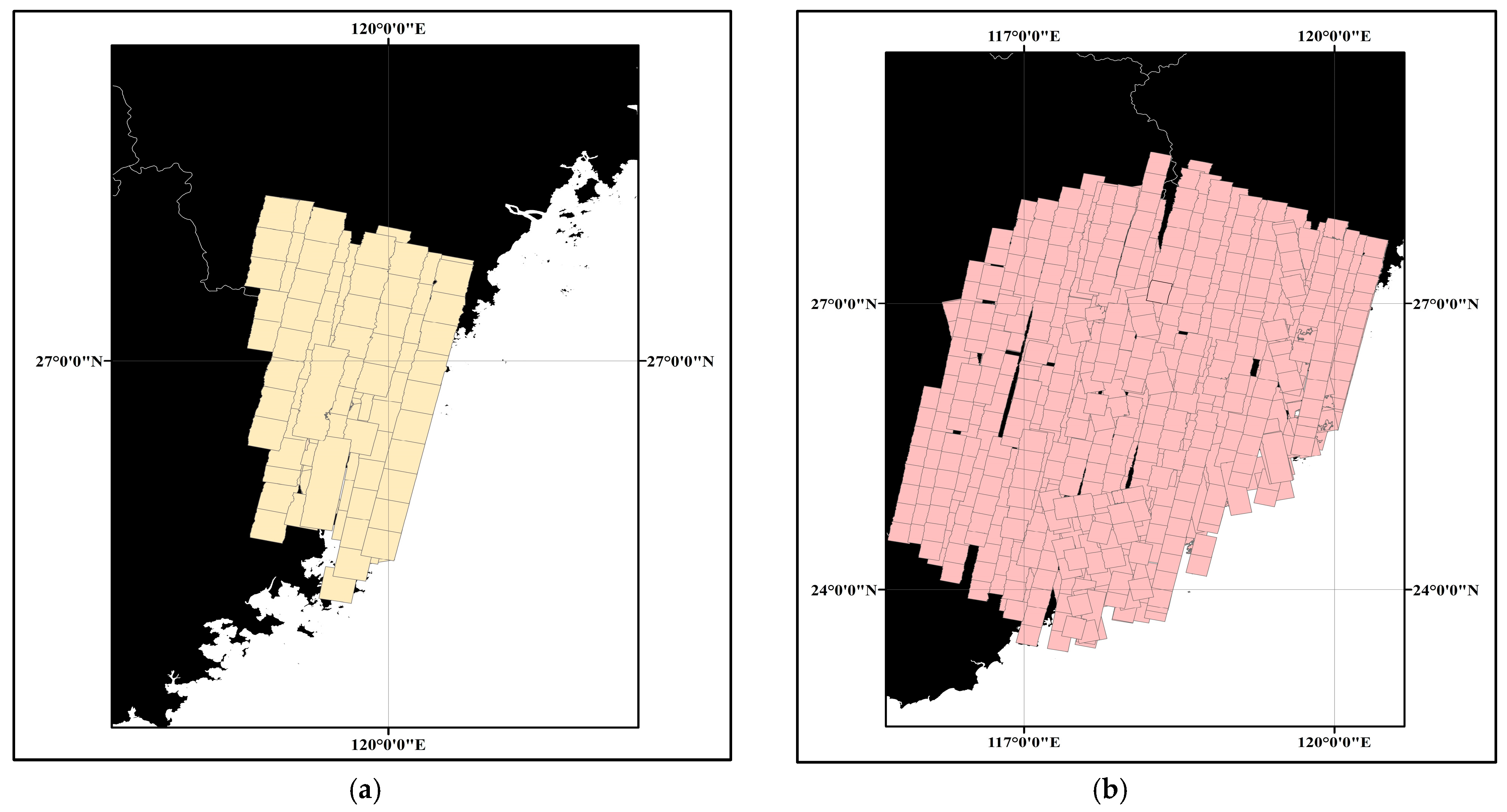
10]. As shown in
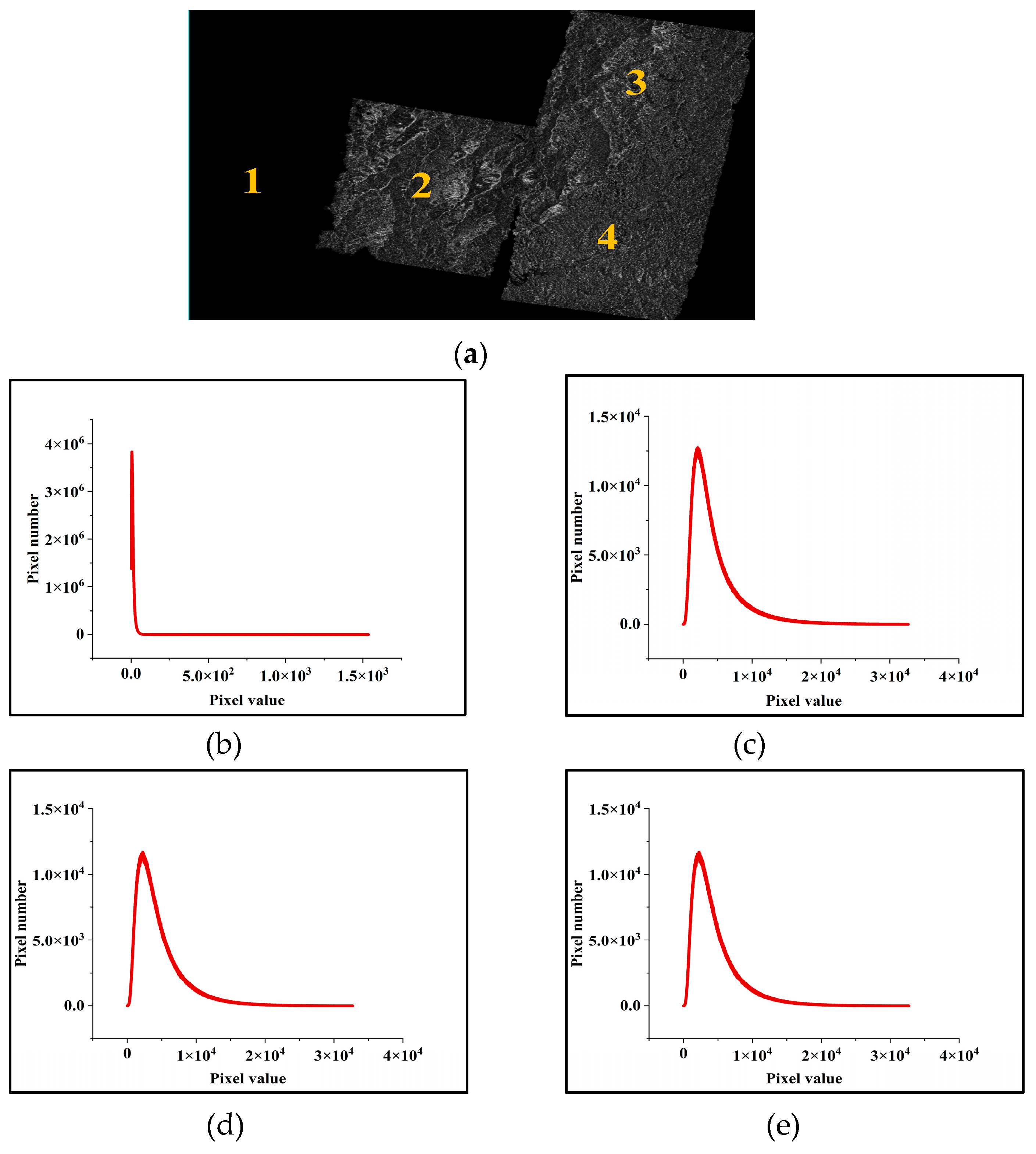
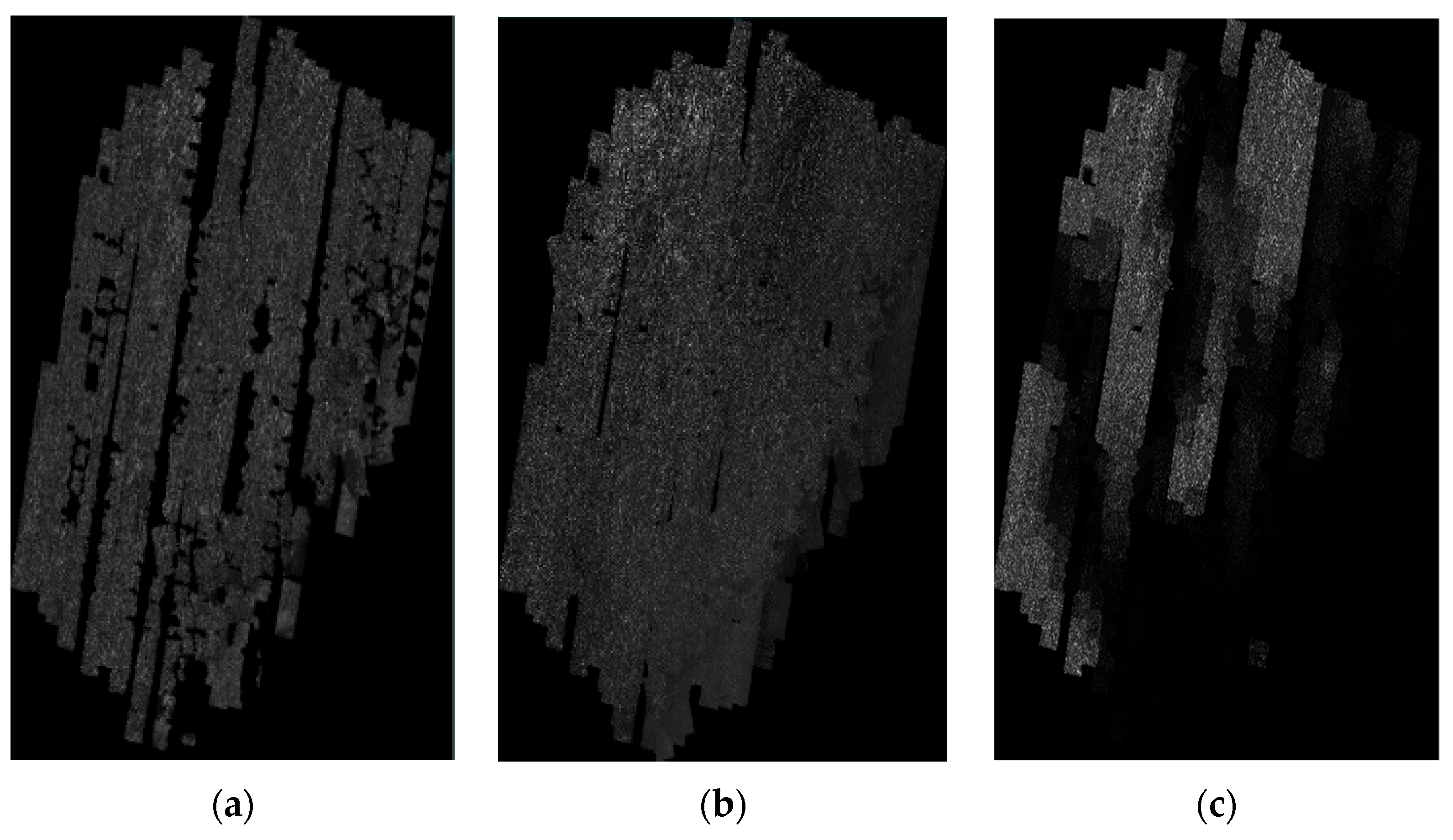
Figure 1a, the brightness anomaly SAR intensity image is darker overall. As shown in
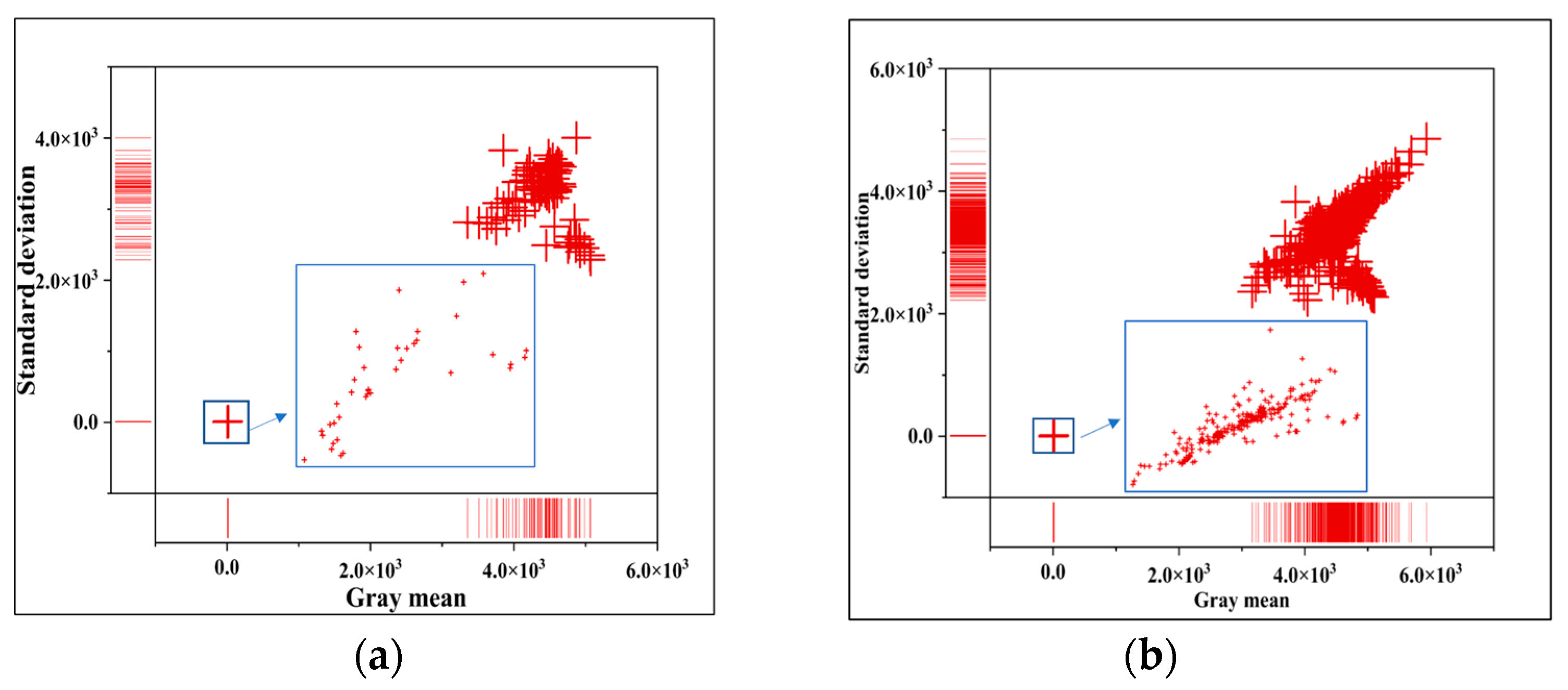
Figure 1b, most grayscale values in the brightness anomaly image are relatively small, with a low gray mean and standard deviation of the image. Although the traditional color harmonization method can resolve color consistency issues in images with brightness anomalies, it may also lead to the loss of brightness information. For instance, the existing color harmonization method determines the stretch parameters of all images by solving a quadratic programming optimization problem [
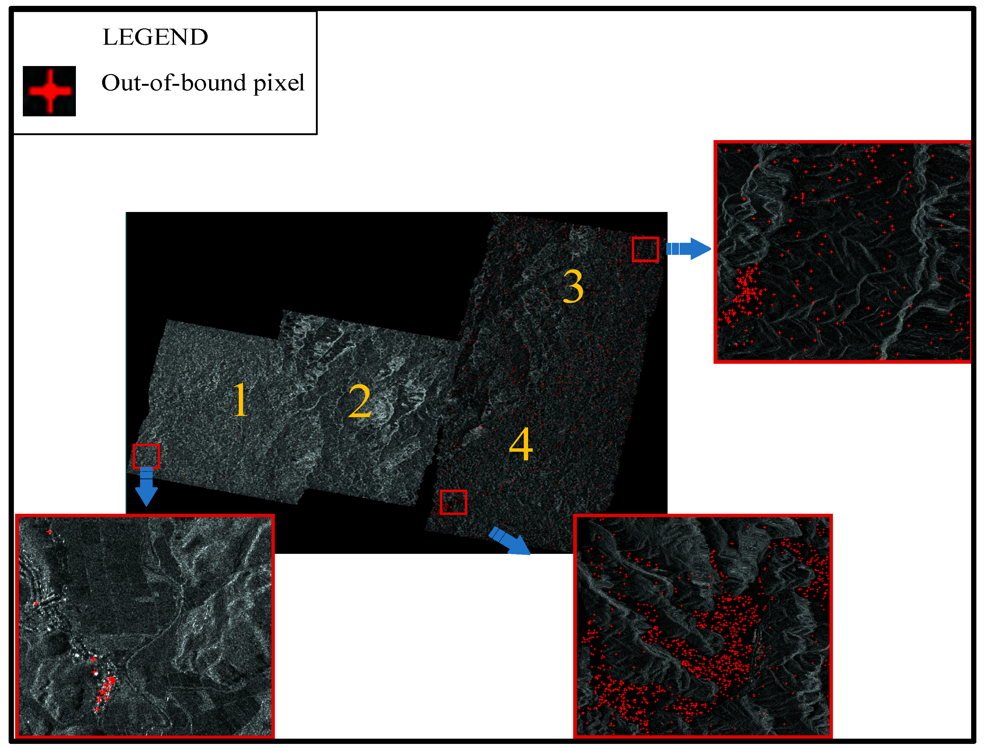
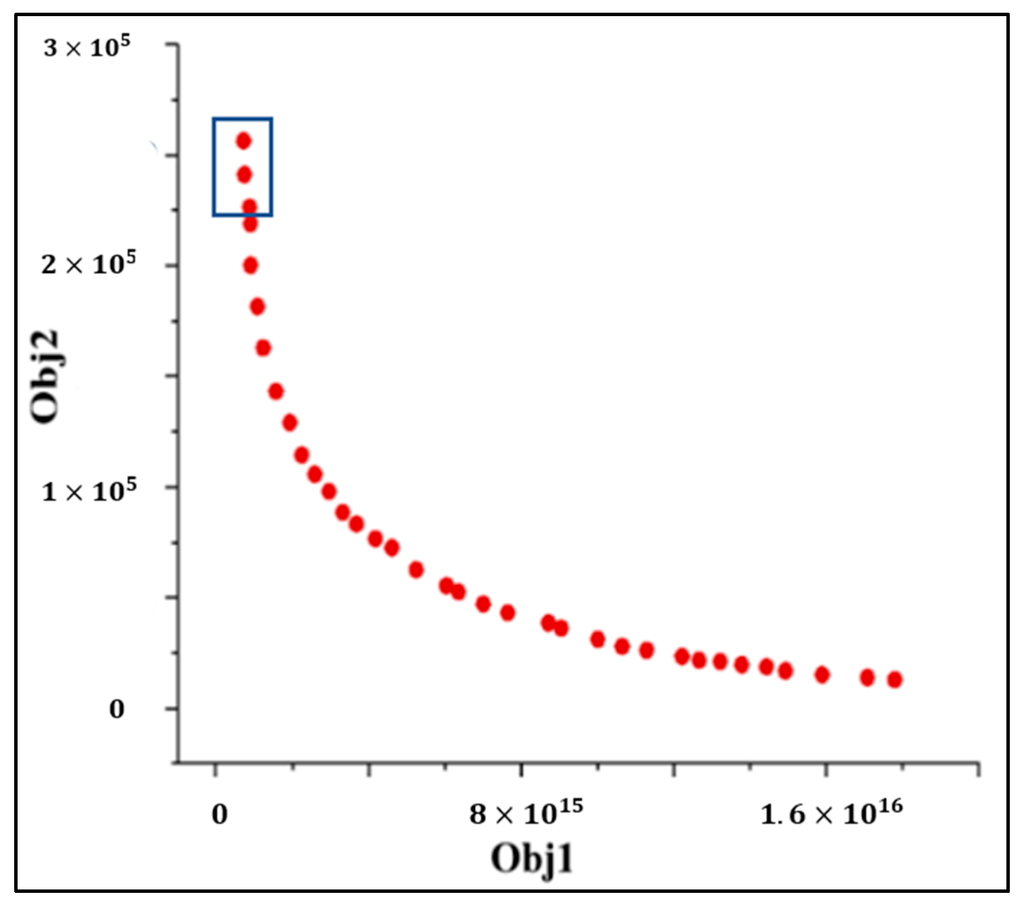
6], which can enhance the gray consistency of SAR intensity images. However, it may also result in grayscale values exceeding the quantization range after image stretching, as shown in the red markers in
Figure 2. The pixel values exceeding the quantization range in the first, third, and fourth images were 559, 14,376, and 10,622, respectively. Typically, out-of-bounds pixel values are directly set to 0 or the maximum grayscale value, leading to the loss of brightness information.
There are few publicly reported methods for the gray consistency of SAR intensity images with brightness anomalies. Most studies have focused on the gray consistency of images without brightness anomalies, preserving image details while optimizing gray consistency [
11], but they have ignored the problem of brightness information loss.
Most current radiometric normalization methods for SAR intensity images have been inspired by optical image processing techniques [
5]. Radiometric normalization approaches for multiple images can be categorized into global, local, or combination models [
7]. The global strategy is a mainstream method [
12]. The global model employs a single function to correct the overall color consistency of intensity images, while the local model uses multiple local functions to eliminate intensity discrepancies in overlapping regions. The combined model leverages both approaches’ advantages, effectively reducing local and global color discrepancies.
Global models often assume that the radiometric relationships between image pairs can be fitted using a linear or nonlinear function [
5]. The least-squares method and linear regression model using pixel pairs in overlapping regions are typically used to process images that require high registration accuracy and slight radiation differences [
11]. The linear model assumes that the intensity discrepancies between different images are characterized by a linear relationship [
6]. To describe the linear relationship between images, researchers have constructed linear models based on pseudo-invariant features (PIFs) [
13,
14,
15]. Nonlinear models, such as histogram matching, align the histograms of two images to achieve similar brightness and contrast characteristics [
16,
17,
18,
19,
20].
The basic principle of a local model is to calibrate local radiometric differences based on regional characteristics [
7]. To eliminate the color differences that exist in local areas and preserve the image gradient information, Li proposed a color-correction model based on a set of local grid linear models [
21]. Tai addressed the problem of local color transfer between two images via probabilistic segmentation using a new expectation maximization (EM) algorithm [
22]. Based on global and local models, some scholars proposed combination models. Yu presented an auto-adapting global-to-local color balancing method in which global optimization transforms the color difference elimination problem into least-squares optimization, and local optimization eliminates the color differences in the overlapping areas of the target images with the gamma transformation algorithm [
23]. To address radiometric normalization (RN) in multiple remote sensing (MRS) images, Zhang proposed a block adjustment-based RN method that considers global and local radiometric differences [
24].
Inspired by previous studies [
5], this paper focuses on a multi-objective gray consistency correction for mosaicking regional SAR intensity images with brightness anomalies. The motivation of this study is to maintain the overall brightness consistency of image pairs in the overlapping regions and reduce the number of out-of-bound pixels. They are used as two objective functions of the multi-objective optimization model, and trade-offs are made between them according to user preferences. The difficulty in controlling information loss arises from simply using the maximum and minimum values of anomalous images as boundaries, as they do not effectively describe the goal of maintaining the number of out-of-bounds pixels. This overly strict constraint limits the feasible domain, and solving for two conflicting optimization objectives becomes challenging. Our method introduces a flexible inequality constraint for a balanced optimization approach. The optimization model can better manage the trade-off between gray consistency and information preservation. The challenge of multi-objective optimization is effectively solved by exploring the boundary of constraint relaxation. The main contributions can be summarized as follows:
- (1)
A multi-objective optimization model for SAR image gray consistency correction is proposed to tackle regional SAR intensity images with brightness anomalies, which simultaneously optimizes gray consistency and brightness information loss;
- (2)
The maximum truncation values of brightness anomaly images in the inequality constraints are formulated as decision variables, optimizing two objective functions through the adaptive adjustment of the constraint relaxation degrees;
- (3)
A hybrid solution framework combining the NSGA-II and QP algorithm is proposed, effectively addressing the complex optimization problem involving multiple constraints and multi-type objective functions.
The remaining sections of this paper are organized as follows:
Section 2 describes the framework of the proposed method, and introduces a detailed description of the multi-objective optimization model and the solution algorithm framework, respectively.
Section 3 and
Section 4 describes the results of the different algorithms and discusses the experimental results. Finally,
Section 5 presents the conclusions.
2. Materials and Methods
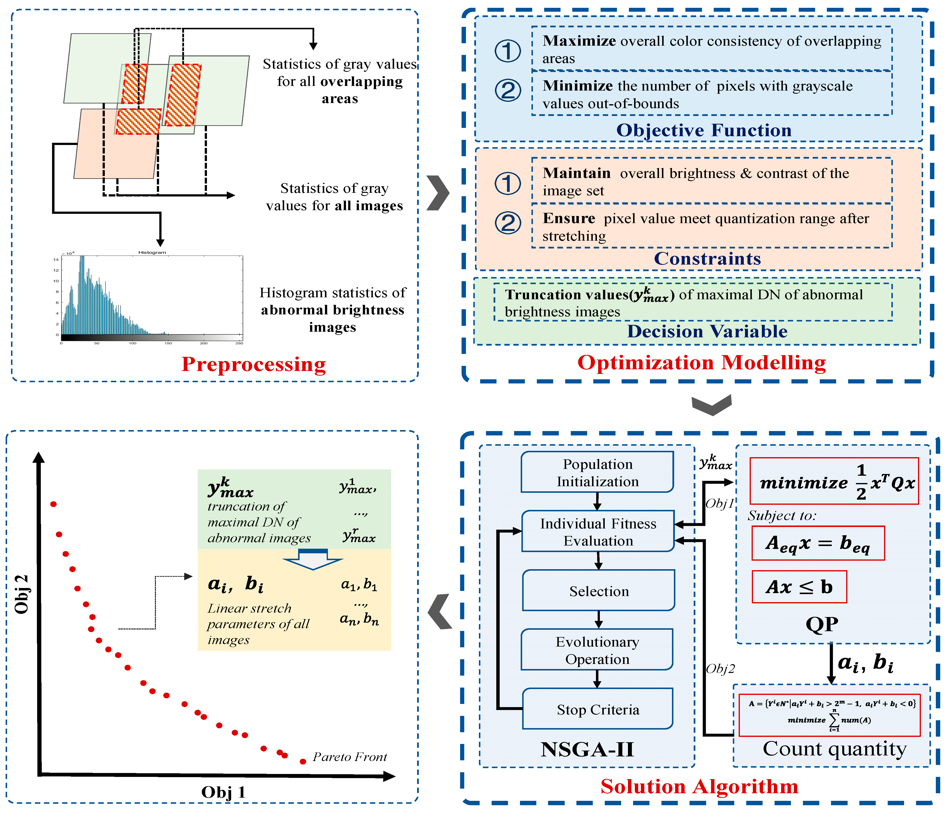
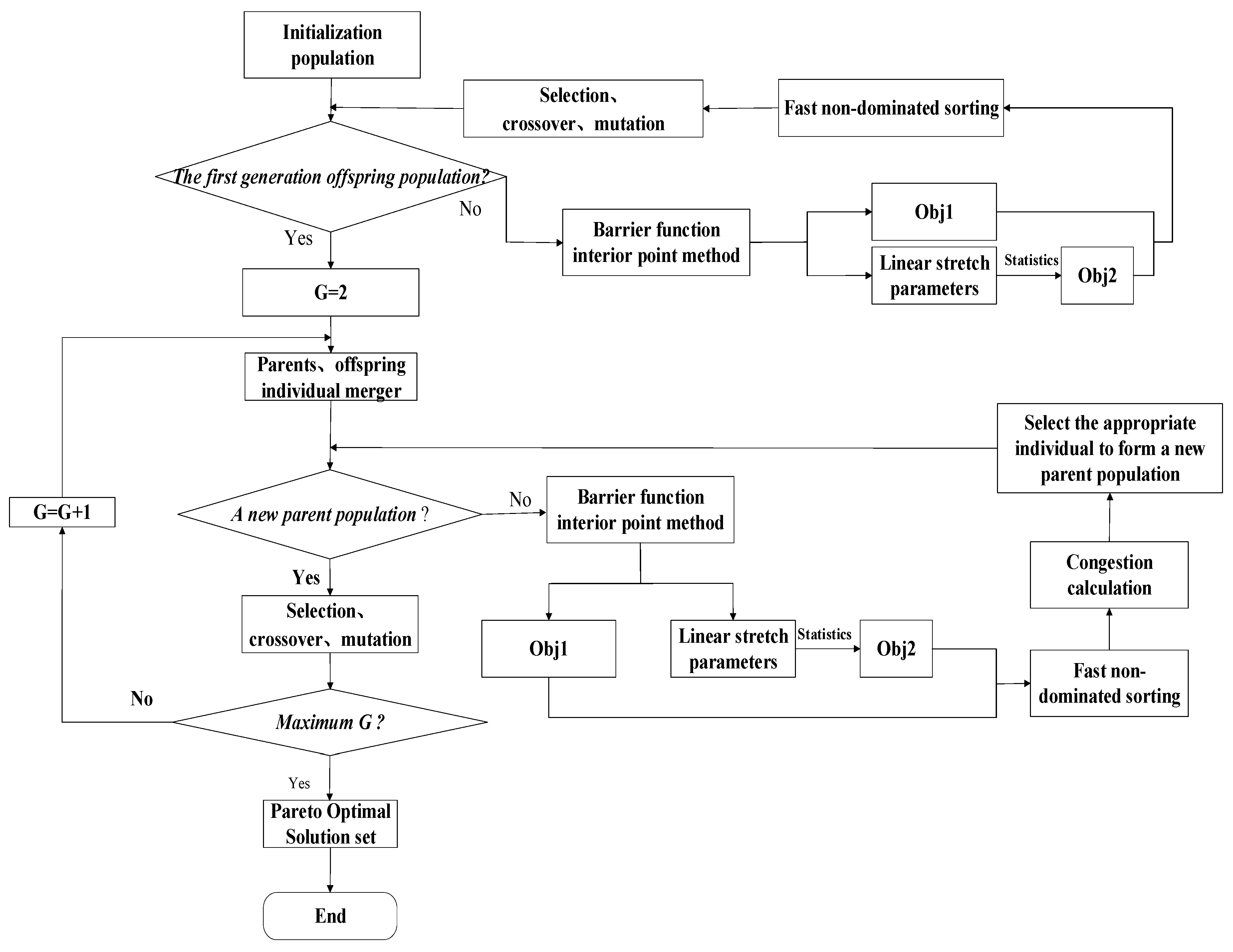
The overall workflow of the proposed method is illustrated in
Figure 3, which comprises three main steps: (1) Data Preprocessing: To obtain the input parameters for the optimization model, the grayscale values of all images, the grayscale values in the overlapping regions of image pairs, and the histograms of the brightness anomaly images were collected. (2) Optimization Modeling: Maximizing the overall gray consistency of overlapping image pairs and minimizing brightness information loss were formulated as two objective functions. The maximum brightness truncation values of the anomalous images were selected as decision variables. The preservation of the overall brightness and contrast of the images before and after processing was considered as an equality constraint. The grayscale values of the images after stretching were kept within the quantization range as inequality constraints. This model formulated the specific problem of gray consistency as a mathematical problem. (3) Solution Algorithm: A hybrid solution framework integrating the NSGA-II [
25,
26] and QP [
27] algorithms was developed to solve the complex optimization model. This framework enabled the simultaneous determination of truncation values for brightness anomaly images and linear stretch parameters for all images. Each solution in the final Pareto optimal front solution set represented a unique combination of stretch parameters for all images and corresponding truncation values for brightness anomaly images.
2.1. Multi-Objective Optimization Model
Equality constraints were set in the traditional color harmonization model [
6], ensuring that the overall brightness and contrast of the image remained consistent after stretching. However, when the dataset contains images with abnormal brightness, relying solely on equality constraints may lead to the loss of brightness information. To overcome this technical challenge, we introduced inequality constraints to control the number of pixels with grayscale values out of bounds. Considering the extreme distribution of pixel values in the abnormal images, the truncated values in the inequality constraint were selected as decision variables. This allows for adaptive ‘relaxation’ of the constraints, achieving a balanced optimization between gray consistency and brightness information loss.
2.1.1. Linear Stretch Model
A gray consistency model was defined for the
original images. In this study, we consider a general linear transformation model by applying linear stretching to the
images, which is [
15]
where
and
are the linear stretch parameters of the image and the variables to be solved;
represents all valid pixel values before linear stretching; and
represents all valid pixel values after linear stretching.
2.1.2. Objective Functions
This study considers two objective functions. Maximizing the overall gray consistency of overlapping areas after stretching is defined as Objective Function 1 (Obj 1). The formula is as follows:
where
and
represent image pairs with overlapping regions;
is the total number of images;
and
are the gray means in the overlapping part of the images
and
after stretching;
and
are the standard deviations in the overlapping part of the images
and
after stretching;
and
are the linear stretching parameters of image
;
and
are the linear stretching parameters of image
;
is the gray mean of the overlapping region of the image
before stretching;
is the gray mean of the overlapping region of the image
before stretching;
is the standard deviation of the overlapping region of the image
before stretching;
is the standard deviation of the overlapping region of the image
before stretching;
is equal to
, which denotes the number of pixels in the overlapping part of the images
and
.
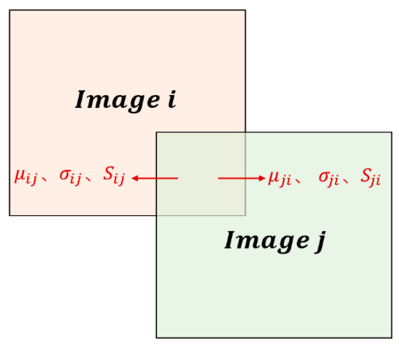
Figure 4 shows the overlapping image pairs.
Let
be the parameter vector of the
images:
. The first objective function can be expressed as a quadratic function of the parameter vector
. The formula is as follows:
is a
matrix, which is equal to
Minimizing the number of pixels with grayscale values that are out of bounds is objective function 2 (Obj 2). The formula is as follows:
where
denotes all pixel values of the image
;
denotes a positive integer,
and
are the linear stretch parameters of image
;
is the number of quantization bits of the original image, the values 0 and
correspond to the minimum and maximum pixel values derived from the quantization range of the image pixel values,
denotes the number of elements in set
A.
2.1.3. Constraints
Equality constraints were established to ensure consistency in the overall brightness and contrast before and after the linear stretching of images. The formula is as follows:
where
denotes the number of pixels in the image
;
is the gray mean of the image
;
is the standard deviation of the image
.
The equality constraints can be expressed as follows:
is a
matrix and
is a vector, which are equal to
Out-of-bounds pixels result in the loss of brightness information. Therefore, it is essential to constrain the pixel values within the quantification range of the image. To prevent out-of-bound pixels after stretching, the following inequality constraints are formulated:
where
and
denote the minimum and maximum pixel values of the original image
, respectively.
The inequality constraints can be defined as follows:
where
is a
matrix and
is a vector, which are equal to
2.1.4. Decision Variables
To control the brightness information loss in the gray correction processing, we introduce the truncation values of the brightness anomaly images as the decision variables to relax the inequality constraints in Equation (21). It is as follows:
where
denotes the truncation value parameter for the
-th abnormal image,
represents the total number of abnormal images.
2.2. Solving Algorithm
This study addresses a multi-objective optimization problem involving two types of objective functions. The first type is a continuous quadratic function, which, together with the constraints, constitutes the QP model. The second type is a discrete nonlinear statistical function. Based on these characteristics of the optimization model, we propose a solution algorithm. Based on the NSGA-II algorithm framework, a set of truncation values for the brightness anomaly images is generated. Once the truncation values are determined, the Obj 1 and linear constraints can be formulated as a QP model. The complexity of solving this model increases significantly with the number of decision variables. The barrier function interior-point method [
28,
29] offers global convergence and numerical stability, making it highly effective for handling large-scale and high-dimensional QP problems. The barrier function interior-point method solves for the linear stretch parameters and Obj 1 values. As the solution approaches the constraint boundaries, the barrier function value increases rapidly, maintaining the optimization process within a feasible region. The Obj 2 value is determined by statistics based on the linear stretch parameters. Pareto optimization [
30] considers the combined effects of multiple objective functions. It can handle optimization problems with conflicting objectives by providing a set of solutions known as the Pareto front, which consists of numerous “non-dominated” solutions. The combination of metaheuristic and deterministic algorithms, through the iterative process of the NSGA-II algorithm, generates a set of Pareto optimal solutions, achieving the integrated solution of truncation values and stretching parameters.
Figure 5 shows the flowchart of the solution algorithm, which can be decomposed into nine steps.
Step 1: Data pre-processing: The following data should be obtained, including the total number of all images , the total number of abnormal images , the maximum pixel value of each image, the minimum pixel value of each image, the gray mean of each image, the standard deviation of each image, the number of pixels of each image, the gray mean and of the overlapping area between images and , the standard deviations and of the overlapping area between images and , and the number of pixels of the overlapping area between images and . To determine the range of values of the decision variable , it is necessary to collect the histogram for all abnormal images.
Step 2: The initial population is generated.
Step 3: The fitness of all individuals in the initial population is calculated.
(1) Calculation of Obj 1: The decision variables (truncation values of the brightness anomaly images) are substituted into the inequality constraints in Equation (21). Equations (7), (17), and (22) are combined to form the QP model. This model is solved using the barrier function interior point method to obtain the stretching parameters and for all images. The value of Obj 1 is calculated using Equation (2).
(2) Calculation of Obj 2: The linear stretch parameters and of all images are substituted into Equation (14) to calculate the total number of pixels that exceeded the quantization range of the images after stretching.
Step 4: Non-dominated sorting, selection, crossover, and mutation operations are performed on the population to form a new offspring population.
Step 5: The parent and offspring populations are merged.
Step 6: Fast non-dominated sorting and crowding distance calculations are applied to the merged population. Individuals are selected from the highest-ranking sorting layers to constitute a new parent population.
Step 7: A new offspring population is produced using selection, crossover, and mutation operations. The new parent population is combined with the latest offspring population to form an updated population.
Step 8: Repeat Steps 6 to 7. The iterations are stopped when the number exceeds the maximum limit.
Step 9: Output the final Pareto-front solutions and terminate the algorithm. Each solution represents a set of stretching parameters for all images and the truncation values of the brightness anomaly images.
4. Discussion
Table 6 and
Table 7 provide a quantitative comparison of the two datasets, which describe the degree of constraint violation for different methods and the number of pixels with grayscale values that were out of bounds. The degree of violation for the two equality constraints is denoted as Eq1_DCV and Eq2_DCV, while the degree of violation for the inequality constraints is represented by Ineq1_DCV and Ineq2_DCV, as shown in Equations (26)–(29). Based on the data presented in both tables, it can be concluded that the QP_EC method exhibits the highest degree of inequality constraint violation and the largest number of pixels with grayscale values that were out of bounds, as it lacks inequality constraints and fails to address the issue of pixel values exceeding the quantization range after stretching. According to the data in
Table 4 and
Table 5, the gray consistency index of the QP_EC method is in the same order as the method proposed in this paper.
The QP_BC method introduces inequality constraints, significantly reducing the number of pixels with grayscale values that were out of bounds. The degree of equality constraint violation is higher than that of the QP_EC method.
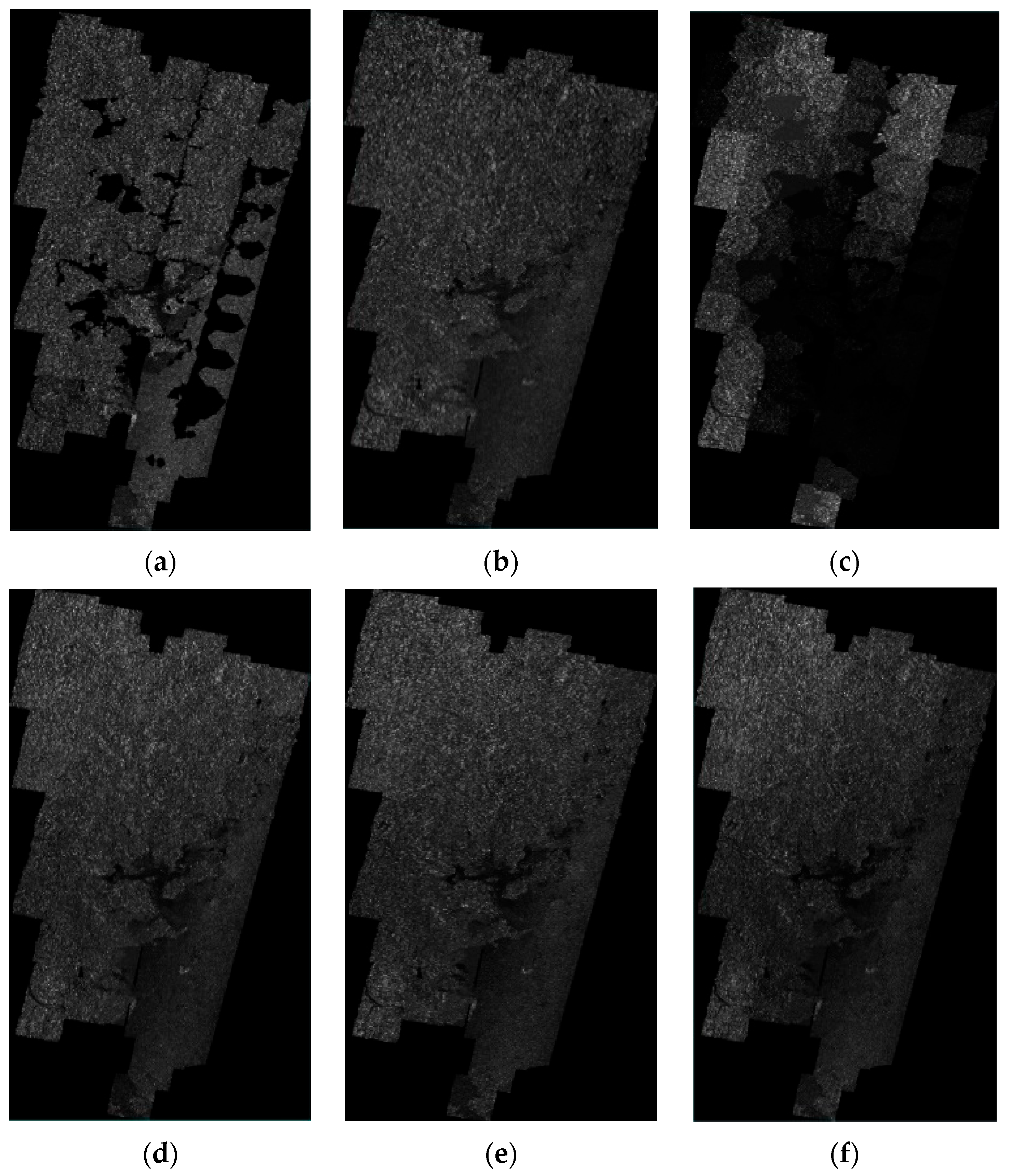
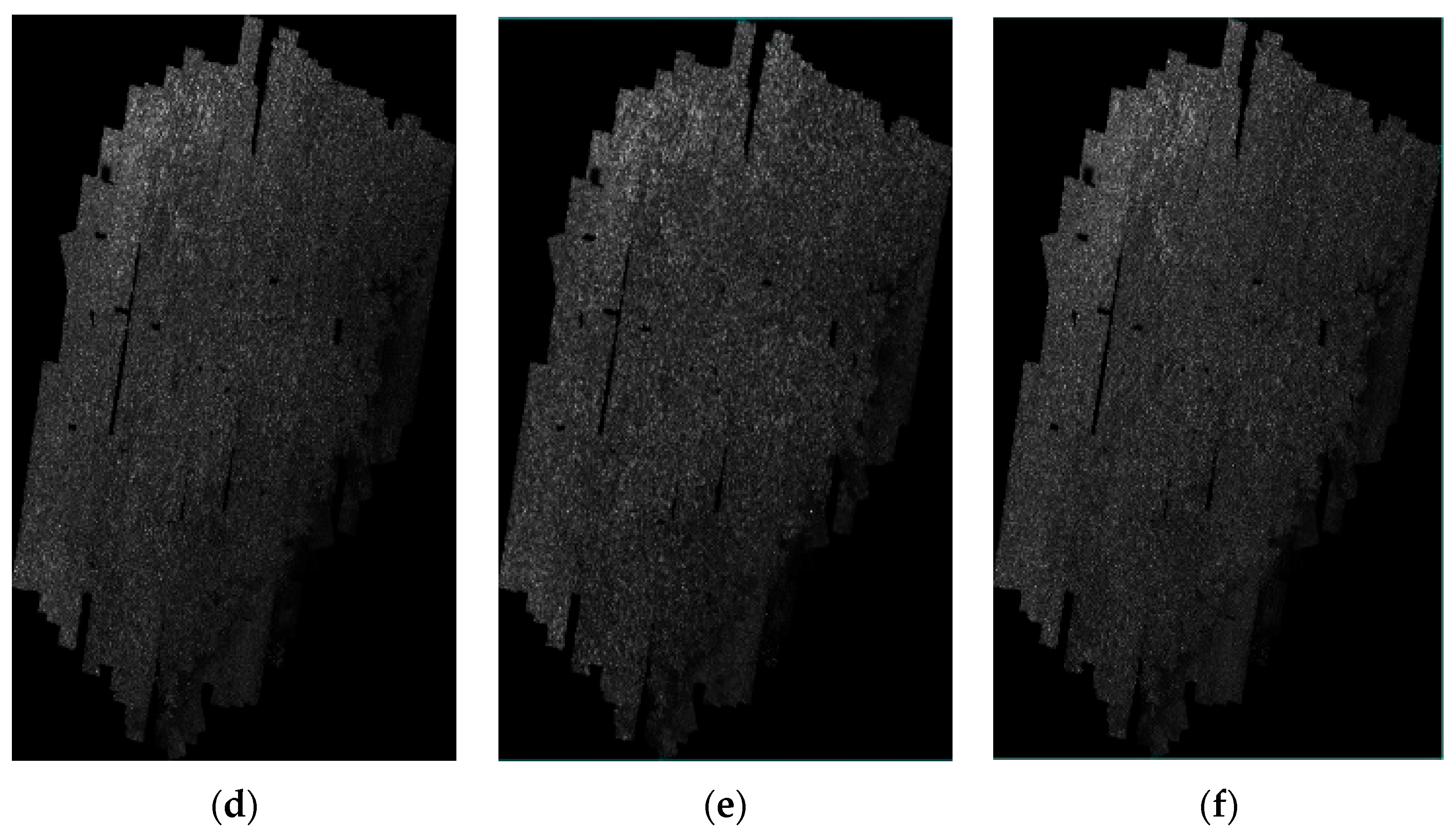
Figure 8c and
Figure 10c show that the continuity between images after stretching is insufficient. According to the data in
Table 4 and
Table 5, the gray consistency index of the QP_BC method is significantly higher than that of the QP_EC method.
The total constraint violation degree of the proposed method is smaller than that of the QP_EC method and larger than that of the QP_BC method. The number of pixels with grayscale values that were out of bounds is smaller than that of the QP_EC method and larger than that of the QP_BC method. The data in
Table 4 and
Table 5 show that the gray consistency index is worse than the QP_EC method but better than the QP_BC method. In this section, we present the analysis of our data based on comparison with the QP_EC and QP_BC methods. Due to the addition of inequality constraints, the degree of equality constraint violation is significantly increased, and the degree of inequality constraint violation is reduced considerably (QP_EC). The degree of equality constraint violation is similar. Owing to the introduction of truncation values, the inequality constraints are relaxed, and the degree of inequality constraint violation is significantly increased (QP_BC). In the first dataset, the proposed algorithm has a low degree of equality constraint violation and a high degree of inequality constraint violation. In the second dataset, the proposed algorithm has a slightly larger degree of equality constraint violation and a higher degree of inequality constraint violation. The QP_BC method adds equality constraints and inequality constraints. Although it can control the number of pixels with grayscale values that were out of bounds, it will significantly decrease gray consistency between images after stretching. Based on the QP_BC method, the proposed method introduces the truncation values to achieve the appropriate relaxation of the solution space and realize the balanced optimization of the two objective functions. The proposed method’s brightness information loss and gray consistency are far superior to those of the QP_EC and QP_BC methods.
5. Conclusions
When regional SAR intensity images exhibit brightness anomalies, balancing gray consistency and brightness information loss becomes a significant challenge in gray consistency processing. Traditional color harmonization methods have struggled to avoid losing brightness information while improving the color consistency of the overlapping regions. We proposed a multi-objective optimization model to deal with this issue, utilizing the truncation values of brightness anomaly images as decision variables. The optimization objectives were to maximize gray consistency in overlapping image pairs and to minimize brightness information loss. The overall brightness and contrast of the images were maintained before and after correction (equality constraints), while the pixel values of the corrected images conformed to the specified range for image pixel value quantization (inequality constraints). Both objective functions were optimized by optimizing the relaxation of the inequality constraints. In terms of the solution algorithm, when faced with multiple constraints, a continuous objective function, and a discrete objective function, this study proposed an algorithm that combined the global search capability of the NSGA-II metaheuristic with the precise solution capability of the QP algorithm. Within the NSGA-II framework, the barrier function interior-point method was used to solve Obj 1 and its corresponding linear stretch parameters. Based on the linear stretch parameters, Obj 2 was computed. The proposed method provided an integrated solution for the truncation values of brightness anomaly images and linear stretch parameters.
Two datasets were used to evaluate the performance and applicability of the proposed method, and comparisons were made with other methods. The experimental results demonstrated that the proposed method effectively maintains gray consistency while significantly reducing brightness information loss. Given the assumption that the overall brightness and contrast of the entire image dataset should be preserved, adaptive handling of equality constraints based on the proportion of abnormal images will be a key focus of future research. In addition, we plan to utilize learning-based methods to achieve the mosaicking of large-scale SAR images with anomaly images.


 ,
, 

