Evaluation of Modified Reflection Symmetry Decomposition Polarization Features for Sea Ice Classification

Abstract

In synthetic aperture radar (SAR) image sea ice classification, the polarization decomposition techniques are used to enhance classification accuracy. However, traditional methods, such as Freeman–Durden (FD) and H/A/α decomposition, struggle to accurately characterize complex scattering mechanisms, limiting their ability to differentiate between various sea ice types. This paper proposes using the Modified Reflection Symmetry Decomposition (MRSD) method to extract polarization features from Gaofen-3 (GF-3) satellite fully polarimetric SAR data for sea ice classification tests. The study data included three types of sea surface: open water (OW), young ice (YI), and first-year ice (FYI). In this research, backscattering coefficients were combined with FD, H/A/α, and MRSD polarization features to create eight feature combinations for comparative analysis. Three machine learning algorithms, Random Forest (RF), Extreme Gradient Boosting (XGBoost), and Support Vector Machines (SVM), were also used for the comparative analysis. The results show that MRSD polarization features significantly improve model performance, particularly distinguishing among sea ice categories. Compared to using only the backscatter coefficient, MRSD polarization features increased model classification accuracy by approximately 4% to 13%, outperforming FD and H/A/α polarization features. The XGBoost model trained with MRSD polarization features achieves excellent classification results, with classification accuracies of 0.9630, 0.9126, and 0.9451 for OW, YI, and FYI. Additionally, the model achieved a Kappa coefficient of 0.9105 and an F1-score of 0.9403. Feature importance and SHapley Additive exPlanations (SHAP) analysis further demonstrate the physical significance of the MRSD polarization features and their role in model decision-making, suggesting that the scattered component power plays a crucial role in the model’s classification decision. Compared to traditional decomposition methods, MRSD provides a more detailed characterization of scattering mechanisms, offering a comprehensive understanding of the physical properties of sea ice. This paper systematically demonstrates the superior effectiveness of MRSD polarization features for sea ice classification, presenting a new scheme for more accurate classification.

1. Introduction

Sea ice constitutes approximately 7–15% of the global ocean area [1], with a primary concentration in the high-latitude waters of the North and South Poles. Its influence on climate, biology, the environment, and ocean circulation is evident at both regional and global scales [2,3,4,5], as well as constraining human activities and operations at sea. Since 1979, the Arctic sea ice melting rate has accelerated in response to global warming, with a concomitant decrease in the sea ice cover year on year [6]. The rapid changes in the sea ice environment and increased human activities in the polar regions drive an urgent need for sea ice monitoring technologies and capabilities [7].

Satellite remote sensing has emerged as an indispensable tool for sea ice monitoring, effectively overcoming the spatial and temporal limitations inherent in traditional observation methods such as fixed stations and ship surveys. Among various remote sensing technologies, synthetic aperture radar (SAR) demonstrates unique advantages through its cloud-penetrating capability, illumination independence, and high spatial resolution [8]. Early-stage SAR-based sea ice classification primarily relied on single or dual polarization intensity combined with texture features [9,10,11,12,13], yet these approaches exhibited inherent limitations in classification accuracy and multi-scale discrimination [14].

Polarimetric SAR (PolSAR), developed based on SAR technology, enables the simultaneous acquisition of multi-polarization backscatter responses, capturing richer physical characteristics of sea ice surfaces. Polarization decomposition enables the polarization information of PolSAR images to be decomposed into different scattering components, thus providing richer information about the scattering mechanism and physical properties of the target or feature surface [15].

Incoherent polarization decomposition is a commonly used method, which can be divided into the eigenvalue-based [16] method and the model-based [17] method. The model-based incoherent polarization decomposition (MIPD) enables quantitative interpretation of scattering mechanisms through mathematical modeling of surface, volume, and double-bounce scattering components. While the pioneering Freeman–Durden (FD) decomposition [17] laid methodological foundations, subsequent studies exposed three critical limitations: overestimation of the volume scattering component [18], occurrence of negative scattering power [19], and the loss of polarization information [20]. Subsequent research has focused on addressing the limitations of the MIPD algorithm. Such as improvements through modified volume scattering models [21] and non-negative eigenvalue constraints [22]. But these methods are oriented to optimize the decomposition algorithm and cannot completely solve the above problems.

Polarization decomposition methods have been used for sea ice classification. Moen et al. [23] developed an automatic sea ice segmentation algorithm using statistical features of backscattering and polarization properties and found that the use of polarization information can improve the sea ice classification accuracy. Lu et al. [24] integrate backscatter coefficients, texture features, and polarization features to train a random forest model for sea ice classification. It is found that polarization features can improve the accuracy of ice and water classification by about 4–10% after controlled experiments. Yang et al. [25] identified the optimal combination of features for fine sea ice classification based on 70 features used in sea ice classification using the separability index method. They found that the fully polarization decomposition parameter performs well in Young Ice identification. Additionally, other studies have employed polarization decomposition to classify sea ice [26,27,28,29]. However, the effectiveness of these methods fundamentally hinges on the ability of the decomposition algorithm to accurately distinguish scattering components. Yet, the inherent limitations of traditional decomposition algorithms often compromise this critical requirement.

An et al. [30] argued that the input to the FD decomposition is not the original measured coherence matrix, but an approximation of the coherence matrix measured under reflection symmetry conditions. This is the main factor that causes the limitations of the MIPD algorithm mentioned above. They developed the Reflection Symmetry Decomposition (RSD) algorithm to solve the negative power and volume scattering overestimating problems of the MIPD algorithm. Subsequently, An et al. extended the RSD algorithm and proposed the modified reflection symmetry decomposition (MRSD) algorithm [31]. The MRSD algorithm effectively addresses the three main limitations of the MIPD algorithm. Its decomposition results allow for the complete reconstruction of the original polarization coherence matrix, exhibiting precise alignment with the theoretical models of volume scattering, surface scattering, and double-bounce scattering. In addition, MRSD can provide richer polarization physical features than traditional decomposition methods.

Overall, MRSD is an excellent polarization decomposition method, although it has not yet been used in sea ice classification. Therefore, this study adopts the MRSD polarization decomposition method to extract polarization features from the fully polarimetric SAR data of the Gaofen-3 (GF-3) satellite and evaluates the usefulness of these polarization features in sea ice classification.

The current predominant trend in sea ice classification research is deep learning models, such as convolutional neural networks, U-Net, ResNet, and their variants [32,33,34]. These models excel at automatically learning complex features and can process large amounts of multidimensional data. However, their lack of interpretability regarding internal decision-making processes and the significant time and computational resources required for training make them less suitable for evaluating the effectiveness of polarization features in sea ice classification.

In this study, we employed three machine learning models—Random Forest (RF), Extreme Gradient Boosting (XGBoost), and Support Vector Machine (SVM)—to evaluate the effectiveness of the extracted MRSD polarization features for sea ice classification. The classes we focused on included Open Water (OW), Young Ice (YI, recently formed ice), and First-Year Ice (FYI, developed from young ice and no more than one year old). We examined how incorporating MRSD polarization features influenced the performance of these three models and compared their results with those produced using traditional methods such as FD decomposition and H/A/α decomposition. Furthermore, we assessed the applicability of MRSD polarization features in classifying sea ice through feature analysis and actual classification results, using the best-performing XGBoost model as our evaluation method.

2. Study Area and Data

2.1. Study Area

The present study encompasses a portion of the Sea of Okhotsk, Tatar Strait, and Soya Strait, where sea ice phenomena are especially pronounced during the winter. Sea ice typically begins to appear in the Sea of Okhotsk in November, reaches its maximum extent around early March of the following year [35], and then gradually decreases until it melts completely, with significant seasonal characteristics. During winter, sea ice can nearly blanket the entire Sea of Okhotsk, with extended coverage extending to the Tatar Strait and Soya Strait [36]. The Tatar Strait connects the Sea of Okhotsk and the Sea of Japan, and its sea ice conditions are analogous to those of the Sea of Okhotsk. Due to the narrow width of the strait and the strong current, ice movement is frequent, resulting in the formation of complex ice conditions [37]. Soya Strait is another significant strait connecting the Sea of Okhotsk and the Sea of Japan. Its sea ice phenomena are similar to those of the Sea of Okhotsk, with ice typically flowing from the Sea of Okhotsk during winter [37]. The geographic location of the study area is shown in Figure 1.

2.2. GF-3 Fully Polarimetric SAR Data

The Gaofen-3 (GF-3) satellite was developed and launched by China in August 2016. It is a civilian remote sensing system equipped with a C-band (5.4 GHz) SAR. This satellite features fully polarimetric capabilities for electromagnetic wave transmission and reception, enabling data acquisition in single-, dual-, and fully polarimetric modes. Its 12 imaging modes offer diversified observational characteristics, with spatial resolutions ranging from 1 m to 500 m and swath widths spanning 10 km to 650 km [38]. Among these modes, the Quad Polarization Stripmap I (QPSI), QPSI, and wave mode provide fully polarimetric data. Notably, the QPSI mode demonstrates exceptional technical applicability due to its high spatial resolution (8 m) and 30 km swath width, which is conducive to the precise classification of sea ice.

This study utilized 18 GF-3 satellite QPSI-mode scenes of data acquired in February 2020, covering key sea ice distribution regions including the Sea of Okhotsk, Tatar Strait, and Soya Strait (Figure 2). This period corresponds to late winter and early spring, characterized by significant sea ice phenomena. Additionally, the data for each scene are unique due to the sea-land segmentation. A stratified sampling strategy was adopted, with 15 scenes allocated for model training and validation, while the remaining three independent scenes were reserved for post-training testing.

Table 1. GF-3 data information for 18 scenes.

ID	Date	Incidence Angle (°)	Center Location	Usage
T1	19 February 2020	35.26–37.09	45°43′N, 142°85′E	Train
T2	19 February 2020	35.25–37.08	45°70′N, 142°92′E	Train
T3	19 February 2020	35.24–37.07	45°97′N, 142°99′E	Train
T4	19 February 2020	35.17–37.00	48°66′N, 143°73′E	Train
T5	19 February 2020	35.17–37.00	48°93′N, 143°80′E	Train
T6	19 February 2020	35.11–36.95	51°08′N, 144°43′E	Train
T7	19 February 2020	35.10–36.94	51°35′N, 144°51′E	Train
T8	19 February 2020	35.09–36.94	51°62′N, 144°59′E	Train
T9	19 February 2020	35.09–36.93	51°86′N, 144°67′E	Train
T10	26 February 2020	35.23–37.17	49°42′N, 141°33′E	Train
T11	26 February 2020	35.22–37.16	49°99′N, 141°50′E	Train
T12	26 February 2020	35.21–37.15	50°28′N, 141°58′E	Train
T13	26 February 2020	35.20–37.15	50°56′N, 141°66′E	Train
T14	28 February 2020	35.25–37.19	55°59′N, 138°90′E	Train
T15	28 February 2020	35.24–37.18	55°88′N, 138°99′E	Train
V1	19 February 2020	35.27–37.10	45°16′N, 142°78′E	Test
V2	26 February 2020	35.23–37.17	49°70′N, 141°41′E	Test
V3	28 February 2020	35.23–37.17	56°16′N, 139°09′E	Test

provides a comprehensive summary of the detailed information associated with each scene data set.

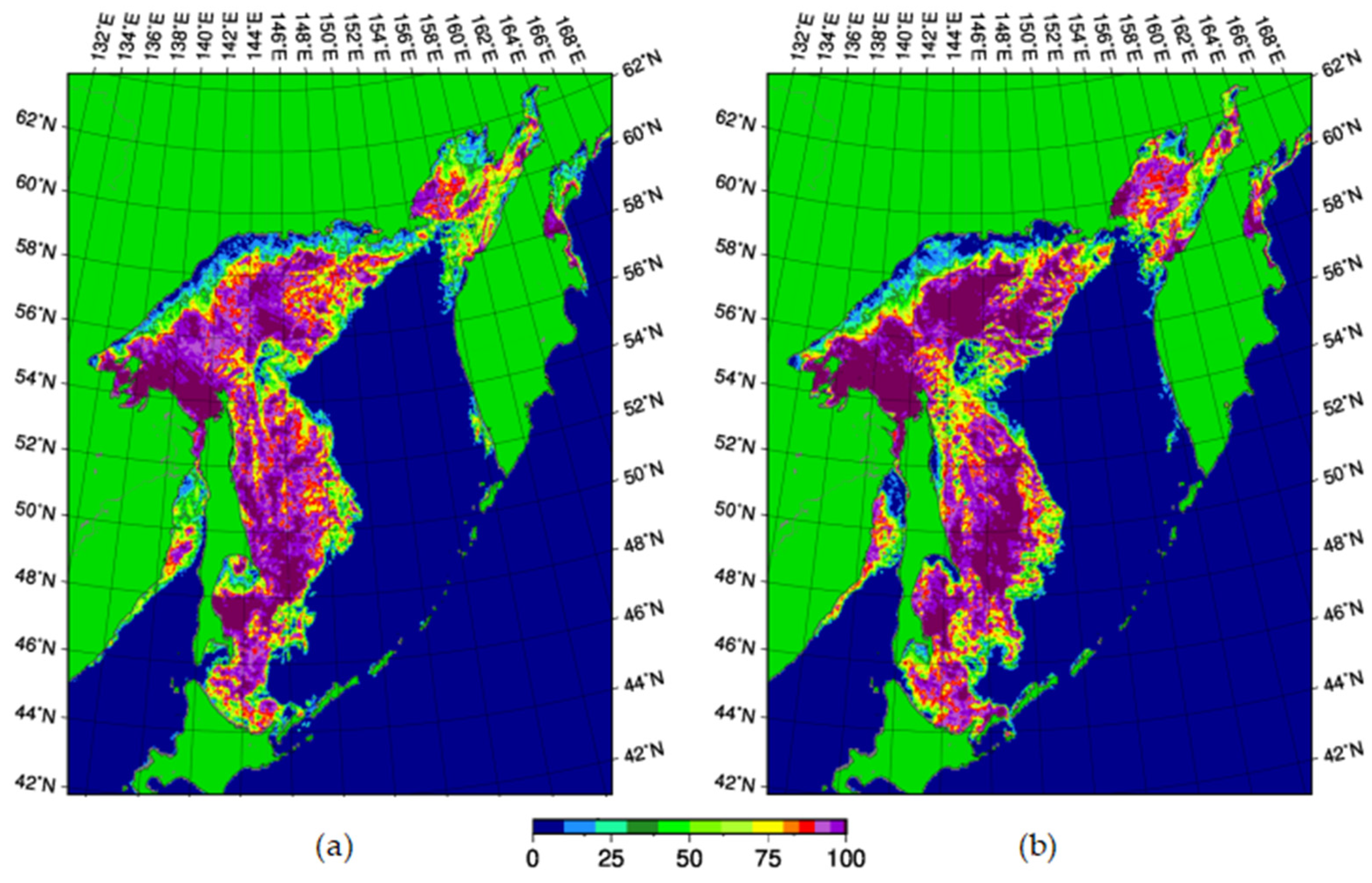
The AMSR2 sea ice concentration dataset in the Sea of Okhotsk, provided by the University of Bremen in Germany (https://data.seaice.uni-bremen.de/databrowser/, data accessed on 6 August 2024), was consulted for this paper. As shown in Figure 2, the Tatar Strait region exhibited sea ice in the melting phase during the study period, while the Sea of Okhotsk and Soya Strait were in the freezing phase. It should be noted that the dataset primarily comprises first-year ice, as multi-year ice types were absent in the study area due to regional sea ice distribution characteristics. Overall, the data employed in this research are relatively comprehensive, except for the sea ice cover type, which excludes multi-year ice.

3. Methodology

3.1. Data Preprocessing

This study employed QSPI-mode Level 1A single look complex (SLC) data, with preprocessing procedures consisting of four main steps: radiometric calibration, true north correction, geometric rectification, and speckle noise suppression. The radiometric calibration was performed according to the formula specified in the GF-3 satellite user manual:

$${\mathsf{\sigma }}_{\mathrm{dB}}=10\times {\log }_{10}\left(P^I\times {\left({\displaystyle \frac{QV}{m}}\right)}^2\right)-K_{\mathrm{d}B}$$

(1)

where σ_dB is the calibrated backward scattering coefficient in decibels and is the sum of the squares of the real and imaginary parts of the single-look complex SAR data, which is also the gray value of each pixel of the magnitude image. QV indicates the maximum pre-quantization value of the image, and K_dB is the calibration constant, both retrievable from the image metadata. The parameter m is set to 32,767, which is specific to the L1A data.

To address the geometric misalignment between SAR image coordinates and real-world geographic coordinates, true north correction was implemented to align the image orientation with the geographic coordinate system, thereby facilitating subsequent manual observation and annotation. The original L1A SLC product exhibits rectangular ground-range pixel dimensions, complicating direct acquisition of accurate image length-width parameters. Furthermore, required corrections of target azimuth angles and other geometric parameters render direct extraction of geometric features in the image domain problematic. This study applied Fast Fourier Transform interpolation-based geometric rectification using underlying geometric relationships to achieve approximately square pixel ground-range dimensions, optimizing conditions for subsequent polarization decomposition. Following these corrections, the scattering matrix was converted into a coherence matrix, after which a non-local means filtering algorithm [39] was employed for speckle noise reduction. This filtering algorithm utilizes the complex Wishart distribution characteristic of PolSAR scattering, selecting homogeneous pixels across extended regions through 3 × 3 neighborhood window comparisons [39], effectively preserving detailed features while suppressing speckle noise. Furthermore, this filtering algorithm enables direct conversion from a single-look image to a multi-look image while maintaining the original image resolution.

3.2. Polarization Features Extraction

The FD decomposition is predicated on the assumption of reflection symmetry, which posits that the scattering properties of targets exhibit symmetry along both horizontal and vertical axes. However, in practical applications, numerous real-world features deviate from this assumption, resulting in reduced accuracy of the decomposition outcomes. In response, the MRSD approach leverages auxiliary data to estimate parameters influencing scattering characteristics, such as the terrain tilt angle. These parameters are employed to refine the reflection symmetry assumption, thereby adjusting the scattering model to more accurately quantify the contributions of distinct scattering components.

The polarization coherence matrix contains the complete information about the polarization scattering of the target. And the non-local means filtering can be directly implemented from single-look image to multi-look image filtering. Each pixel of the multi-look PolSAR image corresponds to a polarization coherence matrix T:

$$T=\left[\begin{array}{ccc}{T}_{11}& T_{12}& T_{13}\\ T_{12}^{*}& T_{22}& T_{23}\\ T_{13}^{*}& T_{23}^{*}& T_{33}\end{array}\right]$$

(2)

This paper uses the MRSD algorithm [31] to extract polarization features from GF-3 satellite fully polarimetric data. Firstly, the reflection symmetric approximation is derived for the polarization coherence matrix T to obtain the three components P_VT_V, T₂, and T₃. The P_VT_V component represents the volume scattering component, while T₂ and T₃ represent the second and third components of the RSD. All three matrices are reflection-symmetric coherence matrices. The specific procedure can be referenced in the literature [30]. Subsequently, nine independent real variables of the RSD decomposition result can be calculated. The variables are P_V, P₂, P₃, 2θ, 2φ, x, y, a, and b. P_V represents the total power value of the volume scattering component. P₂ represents the total power value of T₂. P₃ represents the total power value of T₃. 2θ and 2φ represent the angle information of the orientation angle and spiral angle, respectively, and the range of values is (−π/2,π/2). Similarly, x and y denote the ratio of the spherical scattering power in the components T₂ and T₃, with values in the range (0,1). Furthermore, a and b represent the phase information in T₂ and T₃ and assume values within the range of (−π,π). Further information can be found in

Table 2. Detailed information on MRSD polarization features.

Symbol	Physical Meaning	Formula
PV	Total power value of volume scattering component (Span)	$\mathrm{m}\mathrm{i}\mathrm{n}\left({\mathsf{\lambda }}_1,{\mathsf{\lambda }}_2,{\mathsf{\lambda }}_3\right),{\mathsf{\lambda }}_{\mathrm{i}} \mathrm{f}\mathrm{r}\mathrm{o}\mathrm{m} \mathrm{d}\mathrm{e}\mathrm{t}\left(\mathrm{T}-\mathsf{\lambda }{\mathrm{T}}_{\mathrm{V}}\right)$ ${\mathrm{T}}_{\mathrm{V}}={\displaystyle \frac{1}{4}}\left[\begin{array}{ccc}2& 0& 0\\ 0& 1& 0\\ 0& 0& 1\end{array}\right]$
P2	Total power value of T2	tr(T2)
P3	Total power value of T3	tr(T3)
2θ	Twice the orientation angle	${\displaystyle \frac{1}{2}}{\tan }^{-1}\left({\displaystyle \frac{2\mathrm{R}\mathrm{e}\left({\mathrm{T}}_{23}^{\prime }\right)}{{\mathrm{T}}_{22}^{\prime }-{\mathrm{T}}_{33}^{\prime }}}\right)$
2φ	Twice the spiral angle	${\displaystyle \frac{1}{2}}{\tan }^{-1}\left({\displaystyle \frac{2\mathrm{I}\mathrm{m}\left({\mathrm{T}}_{23}^{\prime }\right)}{{\mathrm{T}}_{22}^{\prime }-{\mathrm{T}}_{33}^{\prime }}}\right)$
x	Power share of spherical scattering in T2	${\mathrm{T}}_2=\left[\begin{array}{ccc}\mathrm{x}& \sqrt{\mathrm{x}\left(1-\mathrm{x}\right)}·{\mathrm{e}}^{\mathrm{j}\mathrm{a}}& 0\\ \sqrt{\mathrm{x}\left(1-\mathrm{x}\right)}·{\mathrm{e}}^{-\mathrm{j}\mathrm{a}}& 1-\mathrm{x}& 0\\ 0& 0& 0\end{array}\right]$
a	RSD second component phase of element T12
y	Power share of spherical scattering in T3	${\mathrm{T}}_3=\left[\begin{array}{ccc}\mathrm{y}& \sqrt{\mathrm{x}\left(1-\mathrm{x}\right)}·{\mathrm{e}}^{\mathrm{j}\mathrm{b}}& 0\\ \sqrt{\mathrm{y}\left(1-\mathrm{y}\right)}·{\mathrm{e}}^{-\mathrm{j}\mathrm{b}}& 1-\mathrm{x}& 0\\ 0& 0& 0\end{array}\right]$
b	RSD third component phase of element T12
PS	Total power value of surface scattering component	$\mathrm{I}\mathrm{f} \mathrm{x}\ge 0.5,\mathrm{y}\ge 0.5,{\mathrm{P}}_{\mathrm{S}}={\mathrm{P}}_2+{\mathrm{P}}_3{,\mathrm{P}}_{\mathrm{D}}=0$ $\mathrm{I}\mathrm{f} \mathrm{x}\ge 0.5,\mathrm{y}<0.5,{\mathrm{P}}_{\mathrm{S}}={\mathrm{P}}_2{,\mathrm{P}}_{\mathrm{D}}={\mathrm{P}}_3$ $\mathrm{I}\mathrm{f} \mathrm{x}<0.5,\mathrm{y}\ge 0.5,{\mathrm{P}}_{\mathrm{S}}={\mathrm{P}}_3{,\mathrm{P}}_{\mathrm{D}}={\mathrm{P}}_2$ $\mathrm{I}\mathrm{f} \mathrm{x}<0.5,\mathrm{y}<0.5,{\mathrm{P}}_{\mathrm{S}}=0{,\mathrm{P}}_{\mathrm{D}}={\mathrm{P}}_2+{\mathrm{P}}_3$
PD	Total power value of double-bounce scattering component

.

Where tr is the trace of the matrix. Re and Im denote the matrix elements of the real and imaginary parts, and T’ = T−P_VT_V, and j denotes the complex unit used to represent the phase difference.

In the RSD algorithm, the constitutive matrix T_A = P_VT_V + T₂ + T₃ represents the original polarization coherence matrix. The surface scattering component P_S and double-bounce scattering component P_D are obtained by Freeman–Durden decomposition. In the MRSD algorithm, T₂ and T₃ are identified as having reflective symmetric forms. Both are consistent with the surface scattering or double-bounce scattering models. P_S and P_D can be derived directly from T₂ and T₃ by applying the rules outlined in Table 2. It is worth noting that, for most pixel points following RSD decomposition, T₂ correlates with double-bounce scattering, while T₃ correlates with surface scattering. P₂ and P₃ are the power values of T₂ and T₃, which provide the scattered component power similar to P_D and P_S. The utilization of P₂ and P₃ may potentially supplant P_S and P_D, thereby offering enhanced insight into the underlying scattering mechanism, a topic also addressed in this study. In conclusion, this study employs the nine polarization parameters derived from MRSD, namely P_V, P₂, P₃, 2θ, 2φ, x, y, a, and b, in conjunction with the P_S and P_D derived from the extension, as polarization decomposition features.

3.3. Sample Generation

After extracting polarization decomposition features, we selected the backscattering coefficients σ_HH, σ_HV, σ_VV, and 11 MRSD polarization features as inputs for model training. These 14 features were normalized to reduce magnitude differences and improve model stability. Then they were stretched to the range of uint16 data (0–65535) to enhance image detail for analysis while meeting precision classification requirements.

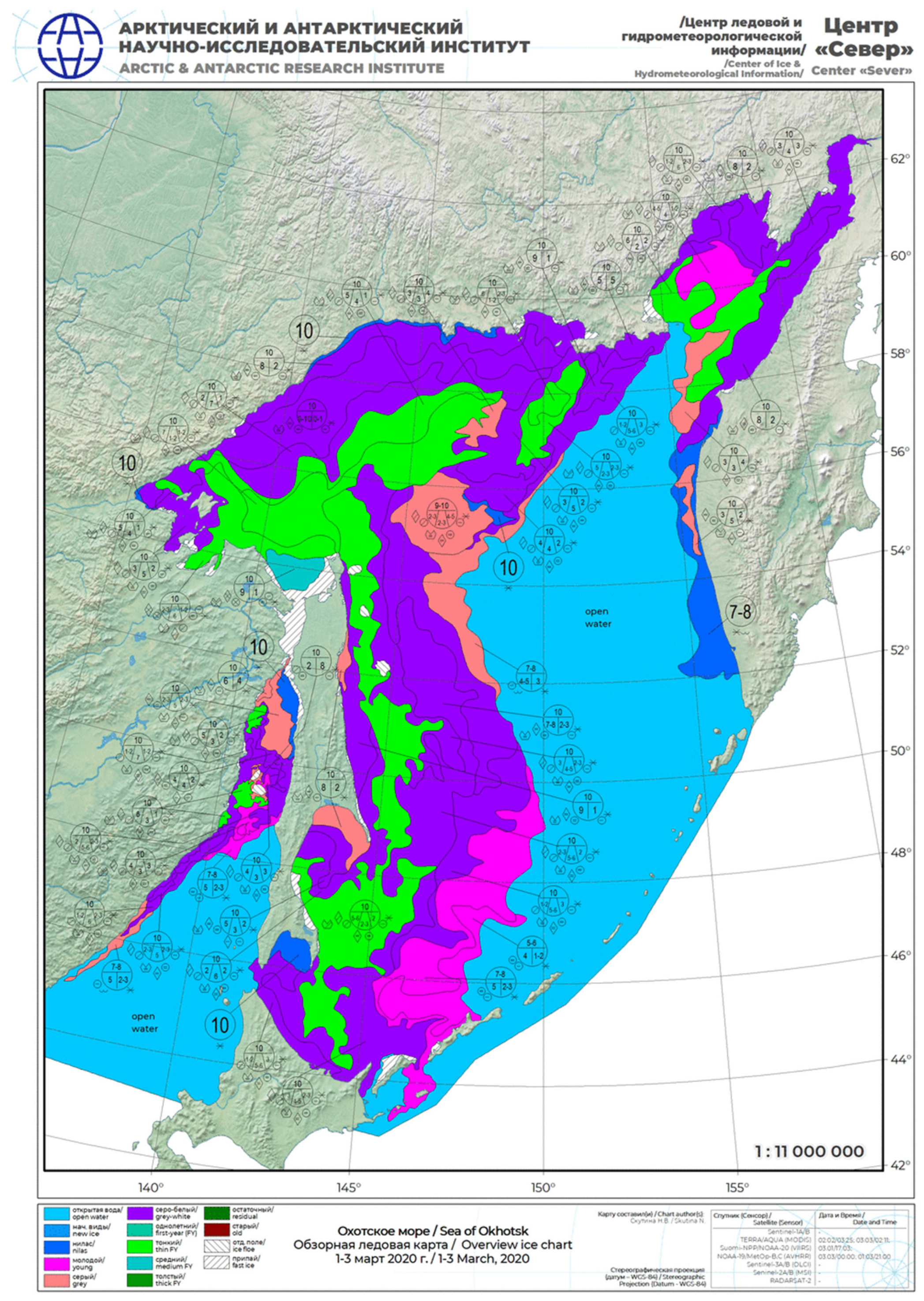
Labeling samples is also an important task, and ground truth is the most authoritative reference for labeling samples. The ice map of the Sea of Okhotsk provided by the Arctic and Antarctic Research Institute (AARI) encompasses the study area delineated in this paper. It offers an ice map with a temporal unit of one month and a spatial resolution of approximately 100 km, which is conducive to the visualization and analysis of large-scale geographic or ice distribution patterns. The resolution of the GF-3 QSPI model data utilized in this study is 8 m, and the ice map provided by AARI is insufficient for the precise classification of sea ice at both temporal and spatial resolutions. However, based on the ice map provided by AARI for 3 March 2020 (https://data.aari.ru/odata/_d0004.php?m=Okh&lang=0&mod=0&yy=2020, data accessed on 6 August 2024), as shown in Figure 3, we deduce that the data mainly cover YI and FYI.

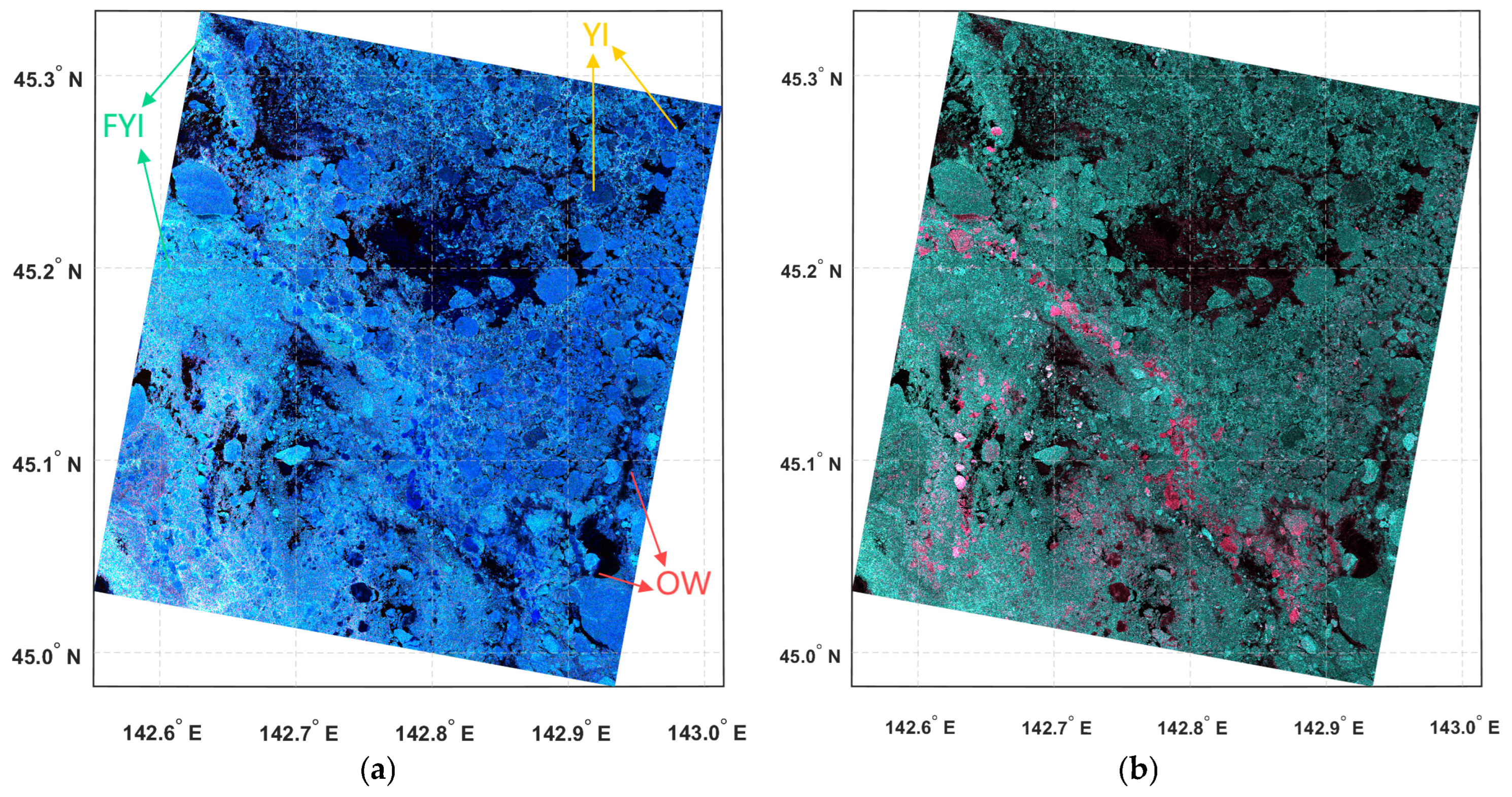
Using SAR or optical remote sensing images directly, it is challenging to distinguish sea ice types by visual discrimination. For this purpose, we reextracted the scattering coefficient S from the preprocessed images to synthesize an RGB reference image for visual discrimination and sample labeling. The RGB image was synthesized as follows: |S_HH − S_VV| for the red channel, |S_HH| for the green channel, and |S_HH + S_VV| for the blue channel. The scattering coefficients contain the amplitude and phase of the L1A level data, calibrated by converting the coefficients so that the square of their absolute value represents the backscattering coefficient. RGB images of red, green, and blue represent the contributions of double, volume, and surface scattering, respectively. Using RGB images, we can improve the visual recognition of sea ice types with distinct colors. S has more complete scattering information (including phase) than backscattering coefficients, which provides richer visual and physical information, enhances visual interpretation, and makes distinguishing between YI and FYI easier. Figure 4 shows the comparative effects of RGB images synthesized using different methods.

In the RGB image, OW appears dark due to weak scattering. YI shows strong surface scattering [40] and a small double-bounce scattering, resulting in a bluish-purple or purplish-red color. FYI is thicker and uniform with strong volume scattering [40], appearing bright cyan or blue. The synthesized RGB image is used as an important reference for labeling. Given the absence of multi-year ice in the selected study area, the samples are classified into the OW, YI, and FYI categories. This is because avoiding forcing the data to make unnecessary age-based distinctions [40] is the only way to realize the model’s full potential in using SAR for sea ice surface feature identification.

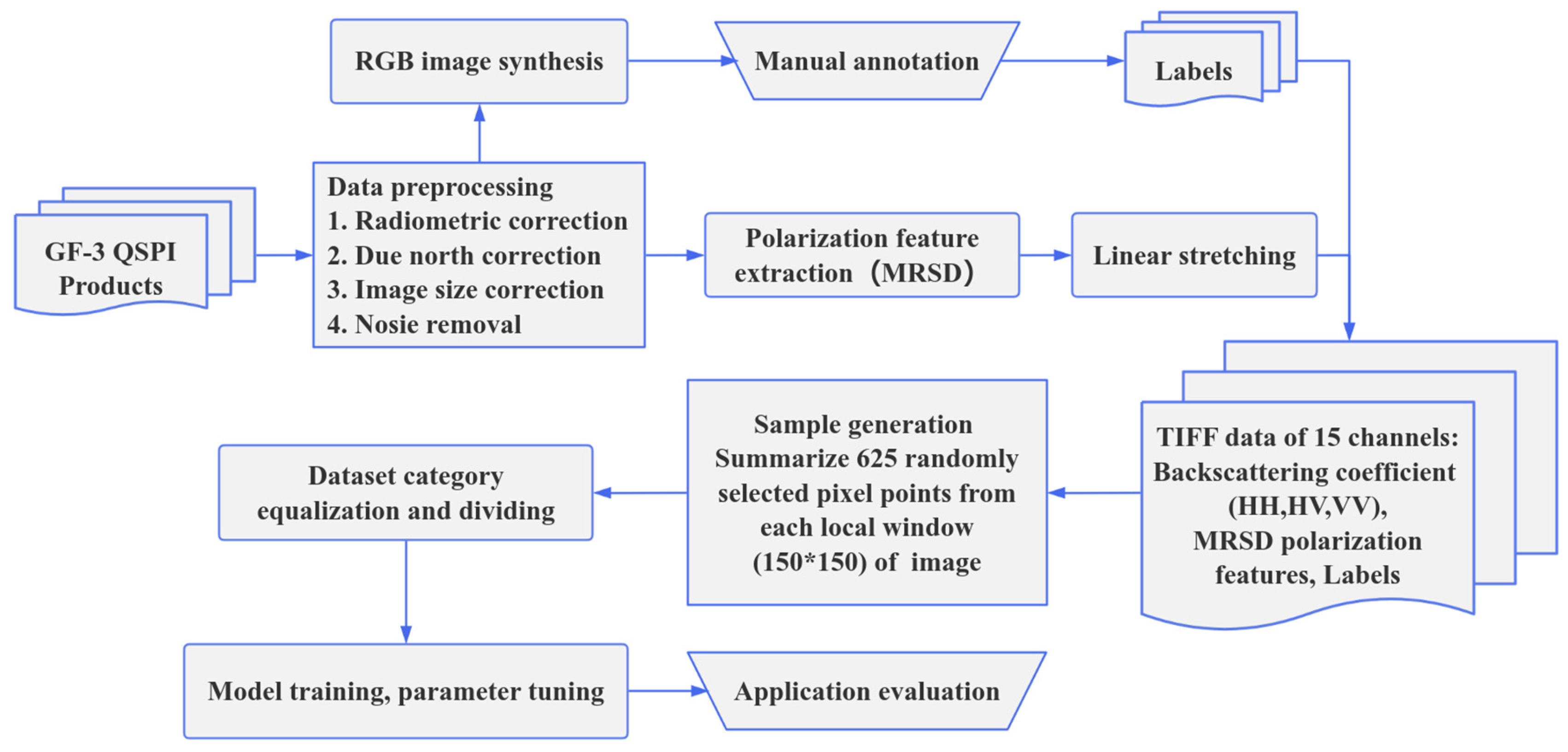
3.4. Model Training

After completing the labeling process, the σ_HH, σ_HV, σ_VV, and 11 MRSD polarization features of each scene dataset are divided into 150-by-150-pixel windows. From each window, 625 pixels are randomly selected as sampling points to minimize redundancy while ensuring enough data for learning. These sampling points are then aggregated and undergo category equalization to maintain adequate representation across all categories, preventing imbalances that could negatively impact model performance. This random sampling method aims to provide diverse training data, enhancing the model’s adaptability to various scenarios. Moreover, the extraction of polarization features typically focuses on individual pixels rather than their relationships with neighboring pixels. This approach allows the model to prioritize independent pixel information, especially when working with rich polarization data. Ultimately, around 13 million samples were generated and divided into training and testing datasets in a 7:3 ratio. The test set data are not included, and all pixels of the image are read for classification to sample pointwise inputs to the model.

The model was subsequently trained on these data, and K-Fold Cross Validation for Hyperparameter Tuning was used to determine the optimal parameter combinations for the model. Application evaluation is performed after training. The overall assessment process in this paper is shown in Figure 5.

4. Application Evaluation

4.1. Model Validation

To evaluate the applicability of MRSD polarization features in sea ice classification, the classical Cloude–Pottier (H/A/α) decomposition [16] and Freeman–Durden (FD) decomposition [17] are employed to extract the H/A/α polarization features (H, A, and α) and the FD polarization features (FP_S, FP_D, FP_V, Fα, and Fβ) for comparative validation. We set up eight combinations of features for comparison experiments: only polarimetric backward scattering coefficients (σ_HH, σ_VV, σ_VV), only polarization features (MRSD, FD, and H/A/α), and a combination of polarimetric backward scattering coefficients and polarization features. All feature combinations train the model in the form of sample points. 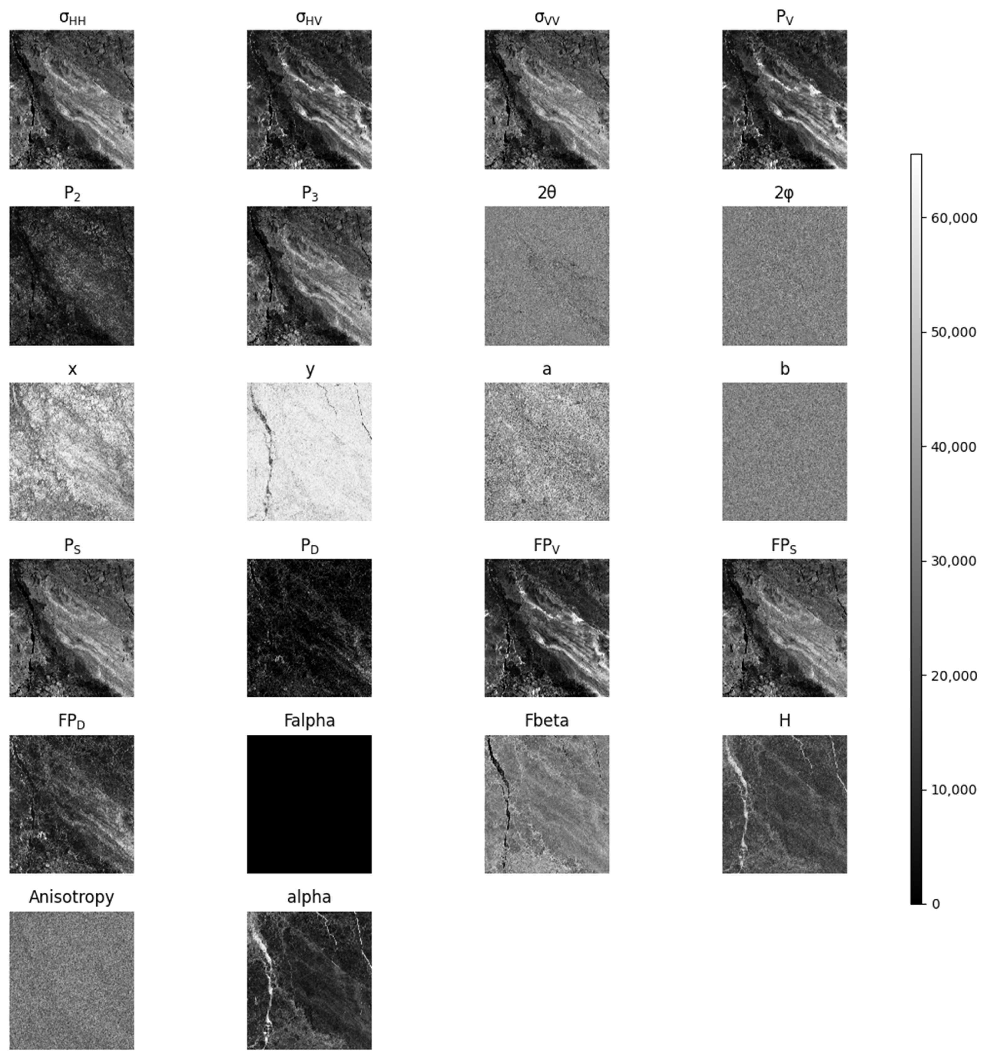Figure 6 shows the grayscale maps of the features utilized in this study, with a 1% linear stretching process applied to enhance visual perception. However, the features were used for model training without linear stretching.

In this study, the same eight combinations of feature data were used to train three machine learning models, including random forest (RF), eXtreme Gradient Boosting (XGBoost), and support vector machine (SVM). RF is an integrated learning algorithm belonging to the bagging type. It constructs multiple decision trees (weak classifiers) and votes or averages their results to obtain a final prediction [41], which gives the overall model a high accuracy and generalization performance. The core idea of SVM is to find an optimal hyperplane in the feature space of the samples to separate the samples of different categories [42], and it is hoped that the hyperplane will maximize the boundary distance of the samples of each category. XGBoost [43] is based on an integrated learning boosting algorithm, whose basic constituent element is also a decision tree, which is optimally classified by a gradient boosting algorithm to form a strong classifier. The XGBoost model is characterized by parallel computational efficiency, overfitting control, and predictive generalization ability. It has also been applied to sea ice classification [44]. In this study, RF and SVM are implemented using Python’s scikit-learn library (version 1.4.2). XGBoost is implemented using Python’s xgboost library (version 2.0.3).

The rationale for establishing comparative experiments in this study stems from the fact that polarimetric backscattering coefficients serve as pivotal discriminative features for sea ice classification, with existing mainstream methodologies being fundamentally derived from the analysis and processing of these parameters. To comprehensively evaluate the performance of the proposed MRSD method, we selected two established benchmarks for comparison: the classical feature decomposition (FD) under the MDPI framework and the eigenvalue-based H/A/α decomposition method. Regarding classifier selection, both Random Forest (RF) and Support Vector Machine (SVM) were included in the comparative study due to their widespread application in sea ice classification research [45,46,47]. The XGBoost model was specifically incorporated based on its superior performance observed in preliminary experiments.

After model training, accuracy (Acc), kappa coefficient (Kappa), precision (Prec), and F1-score (F1-s) were selected as model evaluation metrics. The four evaluation metrics were calculated based on a confusion matrix with the following formula:

$$A\mathrm{cc}={\displaystyle \frac{TP+TN}{TP+TN+FP+FN}}$$

(3)

$$K\mathrm{appa}={\displaystyle \frac{A\mathrm{cc}-P_e}{1-P_e}},P_e={\displaystyle \frac{\left(TP+FP\right)\times \left(TP+FN\right)\times \left(TN+FN\right)\times \left(TN+FP\right)}{{\left(TP+TN+FP+FN\right)}^2}}$$

(4)

$$P\mathrm{rec}={\displaystyle \frac{TP}{TP+FP}}$$

(5)

$$F1-\mathrm{s}={\displaystyle \frac{2\times \mathrm{TP}}{2\times \mathrm{TP}+FP+FN}}$$

(6)

where TP is the sample that was correctly predicted and judged positive, TN is the sample that was correctly predicted and judged negative, FP is the sample that was incorrectly predicted but judged positive, and FN is the sample that was incorrectly predicted but judged negative.

Table 3. Sea ice classification comparison experiments details.

Features Combination	Model	Acc	Kappa	Prec	F1-s
σHH, σHV, σVV	RF	0.7878	0.6816	0.7858	0.7865
	XGB	0.8120	0.7181	0.8090	0.8098
	SVM	0.7832	0.6748	0.7772	0.7771
H, A, α	RF	0.5185	0.2756	0.5126	0.5132
	XGB	0.5213	0.2819	0.5160	0.5180
	SVM	0.5196	0.2794	0.5244	0.5214
FPS, FPD, FPV, Fα, Fβ	RF	0.9160	0.8739	0.9156	0.9157
	XGB	0.9248	0.8872	0.9247	0.9248
	SVM	0.8052	0.7186	0.8042	0.8037
PV, P2, P3, 2θ, 2φ, x, y, a, b, PS, PD	RF	0.9183	0.8774	0.9182	0.9182
	XGB	0.9251	0.8877	0.9249	0.9250
	SVM	0.8164	0.7246	0.8134	0.8144
σHH, σHV, σVV, H, A, α	RF	0.8602	0.7903	0.8588	0.8593
	XGB	0.8614	0.7921	0.8602	0.8605
	SVM	0.7886	0.6829	0.7852	0.7863
σHH, σHV, σVV, FPS, FPD, FPV, Fα, Fβ	RF	0.9257	0.8885	0.9256	0.9256
	XGB	0.9291	0.8936	0.9290	0.9290
	SVM	0.8153	0.7278	0.8138	0.8132
σHH, σHV, σVV, FPS, FPD, FPV, Fα, Fβ, H, A, α	RF	0.9320	0.8980	0.9319	0.9319
	XGB	0.9331	0.8997	0.9330	0.9331
	SVM	0.8187	0.7305	0.8171	0.8170
σHH, σHV, σVV, PV, P2, P3, 2θ, 2φ, x, y, a, b, PS, PD	RF	0.9348	0.9022	0.9346	0.9346
	XGB	0.9403	0.9105	0.9402	0.9403
	SVM	0.8204	0.7306	0.8177	0.8186

details the changes in evaluation metrics for three models trained using various combinations of features. Despite the different classification principles of these models resulting in varied evaluation metrics after training, polarization features significantly improved their classification performance.

Compared with H/A/α decomposition utilizing eigenvalue decomposition, the polarization features derived from FD decomposition and MSRD decomposition, based on model decomposition, significantly enhance model performance. The MRSD polarization features have the greatest improvement in model performance. Compared with the FD decomposition, the MRSD decomposition can obtain eight polarization features except the MIDP three-component, which has an advantage in the number of features. Based on the use of backscattering coefficients, MRSD polarization features improve the model performance better than the simultaneous use of H/A/α and FD polarization features. This indicates that MRSD polarization features provide richer and more meaningful information, which helps the model make better decisions in sea ice classification.

The experimental results indicate that the XGBoost model’s classification performance outperforms the RF and SVM models across various feature combinations. This demonstrates that the XGBoost model can adapt to complex feature spaces and address nonlinear classification problems. Introducing MRSD polarized features notably leads to the optimal classification performance of the XGBoost model. Consequently, we have selected the XGBoost model to explore the applicability of MRSD polarization further features in sea ice classification.

It is important to consider that the incidence angle may influence the MRSD polarization feature. Therefore, we incorporated the backscatter coefficient along with the MRSD polarization feature and the incidence angle as additional training features for the model. However, our findings showed that including the incidence angle did not enhance the model’s performance. This may be attributed to the fact that the incidence angle changes in the fully polarimetric data for each scene within the study dataset are minor (less than 2°) and have little impact on the polarimetric data.

4.2. Features Analysis

4.2.1. Covariance Matrix and Feature Importance

This study further evaluates the applicability of MRSD polarization features in classifying sea ice, focusing on feature analysis utilizing the XGBoost model and its strong performance in real classification tasks. The XGBoost model is optimized by iteratively training multiple decision trees, where training a new decision tree will fit the residuals of the previous training data. The model parameters are set to 650 for the number of estimators (n_estimators), 9 for the maximum depth (max_depth), 0.3 for the learning rate, and 0.1 for the regularization parameter (reg_alpha). These parameters were determined using five-fold cross-validation.

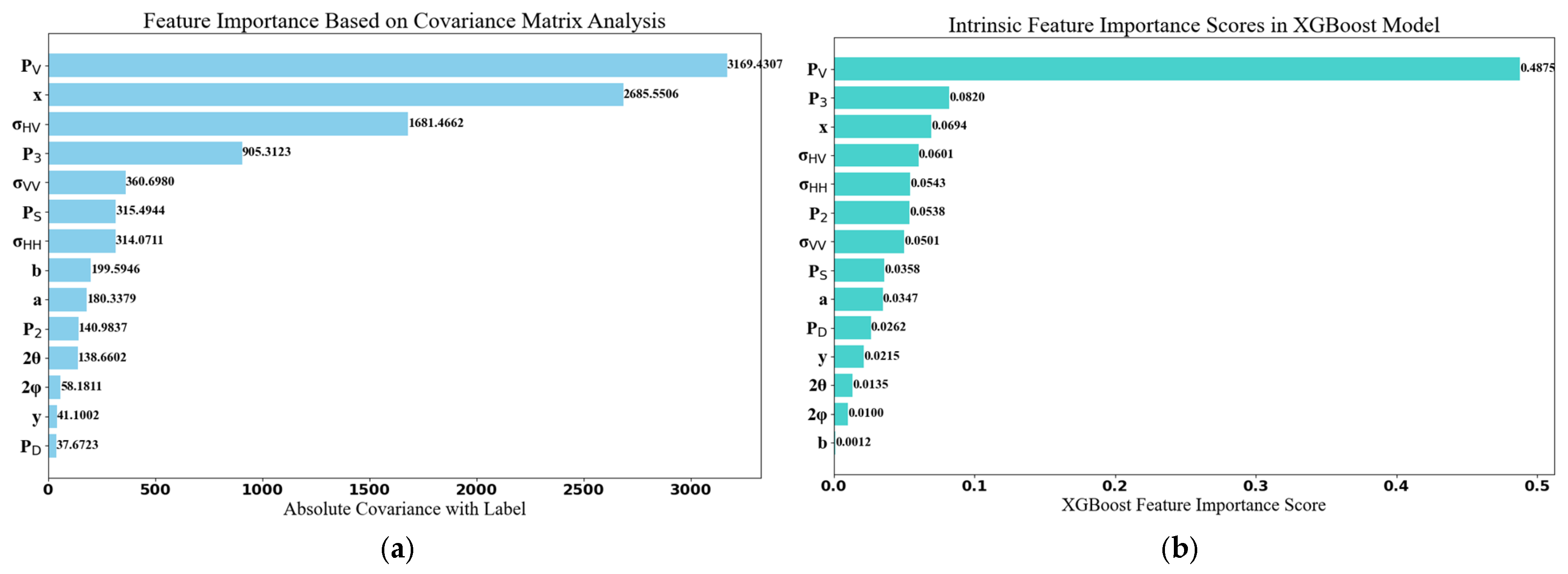
Before model training, we computed feature covariance matrices to investigate linear interdependencies (Figure 7). The analysis identified P_V, x, σ_HV, and P₃ as exhibiting strong linear correlations with class labels, suggesting their potential discriminative power. However, given the potential nonlinear relationships between features and classification targets, we complemented this analysis with nonlinear evaluation methods.

Feature importance indicates how much each feature contributes to the model’s predictive performance. This evaluation considers non-linear interactions between features and their impact on model accuracy. Integrated learning models, such as XGBoost, can provide feature importance scores after training, allowing us to identify which features are crucial for enhancing the model’s predictive accuracy. Figure 7 displays the feature importance scores generated by the XGBoost model. Regarding feature importance scores, P_V is the feature that has the greatest impact on model classification, followed by P₃, x, and σ_HV, in that order. This finding aligns closely with the results from the covariance matrix calculation. However, for other features, there were discrepancies between the results of these two analyses. P_S and P_D, the three components of MIPD, have traditionally been recognized as the primary polarization features. Despite their relatively low feature importance scores in our experiment, they maintain high values in the covariance matrix analysis, suggesting that they still hold significant relevance.

Combining the results of both analyses, we observe that some MRSD polarization features, such as x, P₂, and P₃, contribute more strongly to the model than the three-component MIPD. This indicates that MRSD polarization features provide rich and valuable information. Moreover, these MRSD features offer more detailed insights into the physical structure of sea ice than traditional three-components MIPD, thereby enhancing classification accuracy. Furthermore, the MRSD polarization features possess strong physical interpretations, which can be beneficial for understanding how sea ice’s freezing and thawing processes affect electromagnetic scattering in practical classification tasks.

4.2.2. SHAP Analysis

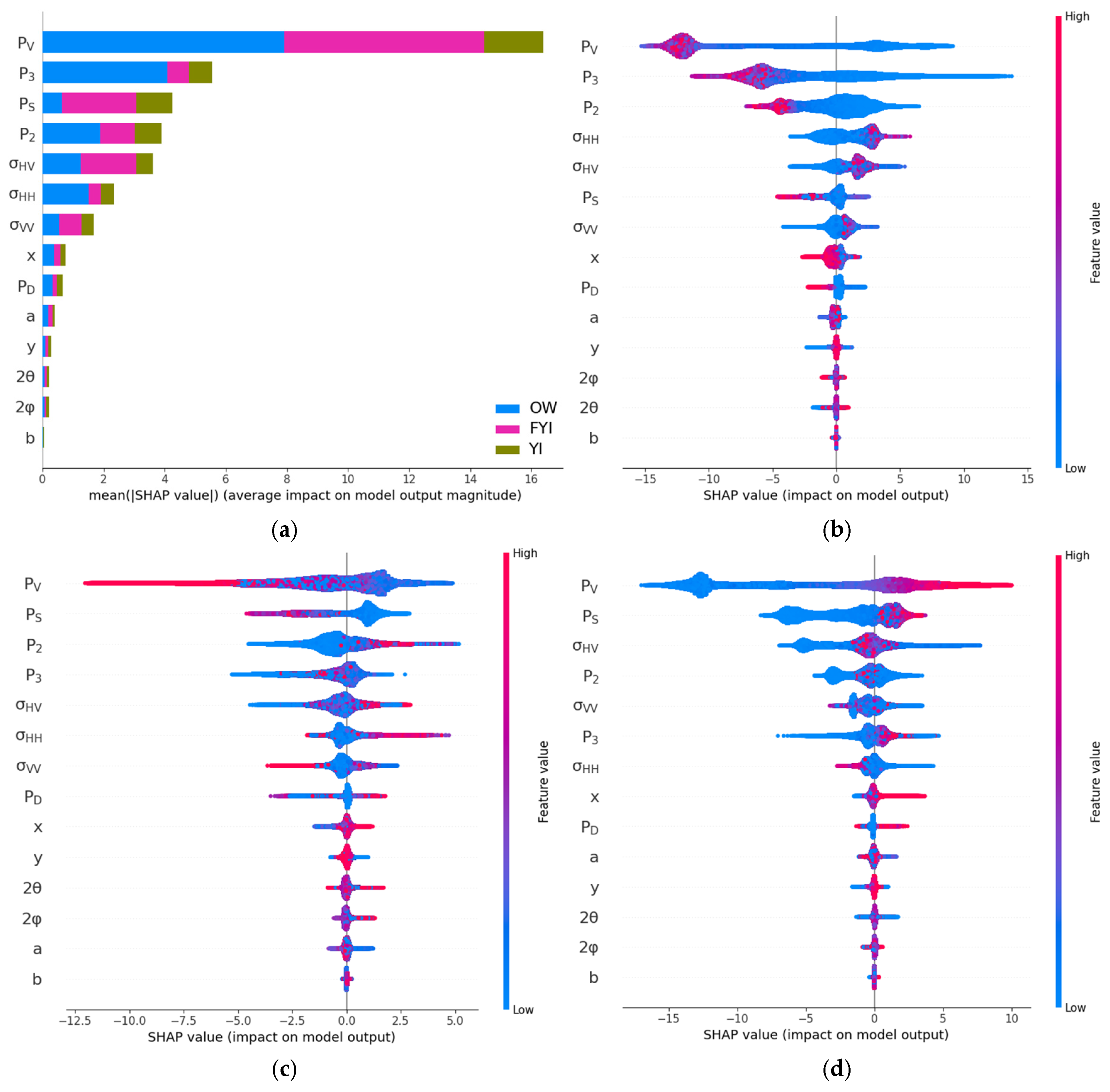
To further elucidate the role of each feature in the model, this study employs the SHapley Additive exPlanations (SHAP) analysis to assess the applicability of MRSD features in sea ice classification. This approach is based on the game-theoretic Shapley values to assess the contribution of each feature to the model’s prediction results [48] and is also an emerging method to explain how the model makes predictions.

SHAP analysis can provide various plot analysis results to measure each feature’s contribution to the model’s predicted value. In particular, the bar plot displays each feature’s average absolute SHAP value, quantifying the magnitude of each feature’s contribution to the model’s predictions. The higher the average absolute SHAP value, the more influential the feature is, basically replacing the traditional feature importance score. The beeswarm plot reveals the actual relationship between the features and the model prediction results; the positive and negative relationship between SHAP values can indicate the gain of features in the model decision category (SHAP value is greater than 0, positive influence, and the opposite is true for SHAP value less than 0). The beeswarm plot also ranks the features in descending order (i.e., the importance of the features is ranked in descending order) according to the sum of the SHAP values of all the samples, which allows us to judge the role of the features when the model predicts a certain category.

Figure 8 illustrates the results of SHAP analysis for the sea ice classification of this study’s dataset. In the three classification tasks, SHAP analysis generated the respective beeswarm plots for OW, YI, and FYI, which visually present how the MRSD polarization features affect the decision of the classification model. For example, in the beeswarm plot for OW, the high values of features that provide the power of the scattering component, such as P_V, P₃ (surface scattering in most pixel points), P_S, and P₂ (double-bounce scattering in most pixel points), are concentrated on the left side of the image, indicating that these features negatively affect the classification of OW. In practice, it is shown that the scattering component in OW is weak or even almost absent, which is consistent with the decision logic of the model, indicating that the MRSD polarization features enable the model to capture the scattering characteristics of sea ice reasonably well.

The results of the SHAP analysis indicate that P_V is the feature most significantly contributing to the model’s predictions, particularly in classifying YI and FYI. Volume scattering can effectively reflect the complex scattering behavior of electromagnetic waves by the internal medium of sea ice. YI has irregular structures such as air inside because it has not been fully compacted, while FYI has more significant body scattering characteristics for both due to its higher density and thickness. The high contribution of P_V further validates the critical role that volume scattering features play in representing the internal structure of sea ice.

Meanwhile, the surface scattering features (P₃ and P_S) also play an important role in the classification. The beeswarm plot shows that the surface scattering features have a strong negative contribution to the classification of OW, which effectively reflects the geometrical properties of OW. The influence of surface scattering is enhanced in YI and FYI, providing important information on ice surface roughness and thawing. In addition, the contribution of P₂ (double-bounce scattering) is relatively high in the FYI classification. This may be attributed to the greater thickness and higher internal densities of the FYI, resulting in a more complex double scattering behavior of the electromagnetic waves on its surface and inside, which enhances the classification model’s ability to discriminate between FYI. In contrast, while contributing less to the overall model, the other features in the MRSD polarization feature also enhance the model’s overall performance by capturing additional information such as geometry and scattering ratio.

Among the MRSD polarization features, P₂ and P₃ provide similar information about the scattering components as the conventional three-component MIPD model (P_D and P_S). Still, they contribute more effectively to the overall model than P_D and P_S. We conducted two comparative experiments to verify this: the conventional three-component MIPD (P_V, P_D, P_S) and the other that employed the three-component (P_V, P₂, P₃). The experimental results presented in

Table 4. Comparative experiments on model enhancement by MRSD polarization features.

Model	Features	Type	Precision	Accuracy	Kappa
XGBoost	σHH, σHV, σVV, PV, PS, PD	OW YI FYI	0.9226 0.8356 0.8806	0.8807	0.8210
XGBoost	σHH, σHV, σVV, PV, P2, P3	OW YI FYI	0.9577 0.8963 0.9243	0.9263	0.8895
XGBoost	σHH, σHV, σVV, PV, P2, P3, 2θ, 2φ, x, y, a, b, PS, PD	OW YI FYI	0.9630 0.9126 0.9451	0.9403	0.9105

clearly show that the combination of P_V, P₂, and P₃ outperforms the traditional three-component MIPD. This indicates that P₂ and P₃ better capture detailed double-bounce and surface scattering information than P_D and P_S. This finding suggests that P₂ and P₃ could be critical features for future models aimed at understanding these scattering phenomena.

Overall, the SHAP analysis highlights the importance of P_V, P₃, P_S, and P₂ features in the classification process. These features improve the model’s classification performance and align with the principles of electromagnetic scattering theory, confirming their physical significance. Moreover, the secondary features play a supportive role, further strengthening the model’s robustness. These findings underscore the applicability and interpretability of MRSD polarization features in the task of sea ice classification, providing a solid foundation for future studies on polarization features.

4.3. Classification Performance

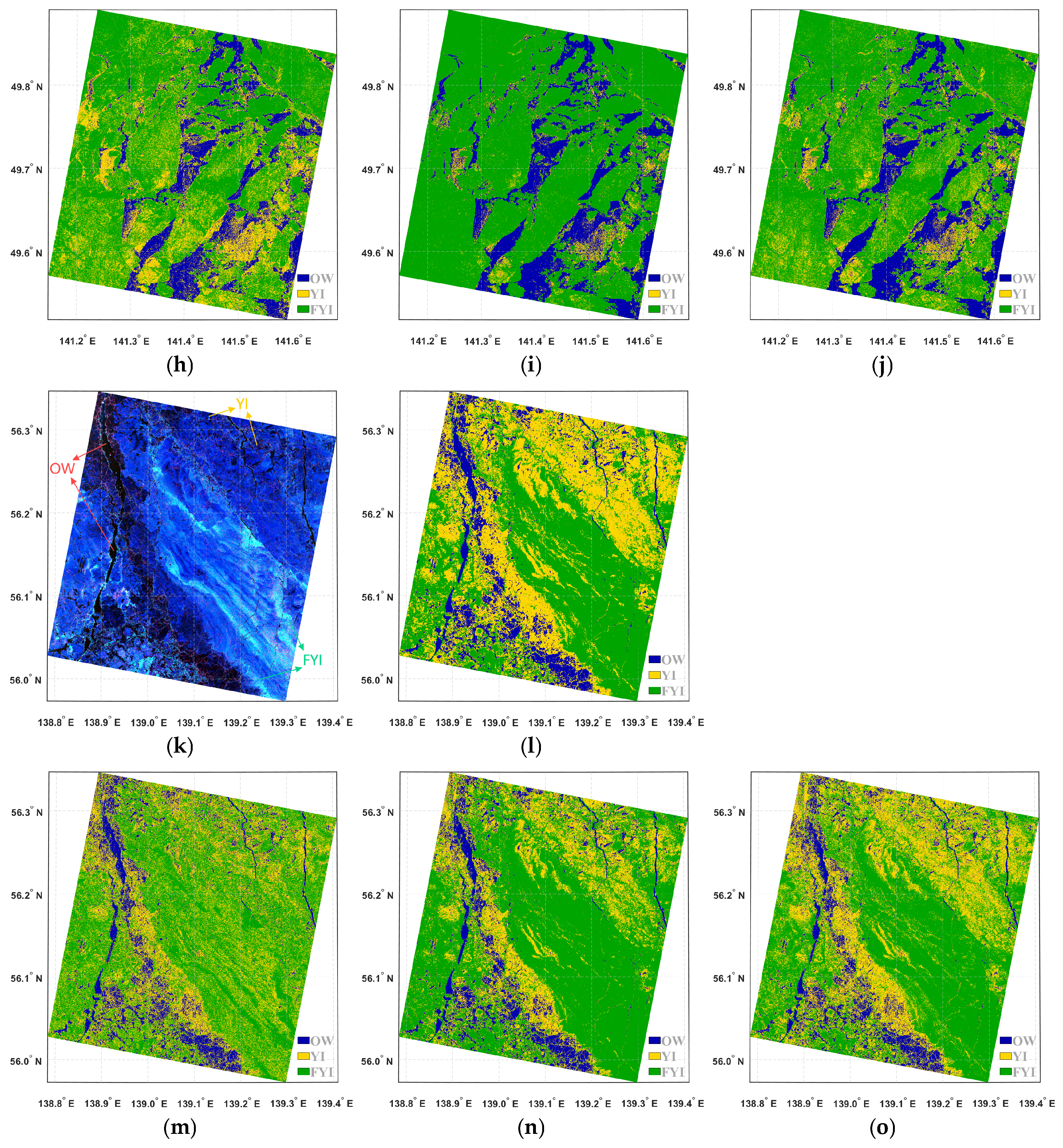
In this study, we finally use backscatter coefficients (σ_HH, σ_HV, σ_VV) with MRSD polarization features to train the XGBoost model. And verify the applicability of MRSD polarization features in sea ice classification by using actual classification results. For a comprehensive comparison, we also used FD and H/A/α polarization features to train the same model for comparison. When the trained models are classified, we calculate the maximum prediction probability of each pixel point as its confidence level and aggregate the average confidence level for each category. The average confidence level can assess the reliability and classification stability of the model in different category recognition tasks as a whole. The role of MRSD polarization features is illustrated below by the actual classification results of the XGBoost model in three scenes of test data. The model performance and classification results are shown in Table 3,

Table 5. Confidence of model identification for each sea ice class after training the model with different polarization features.

Features (XGBoost)	Sence	OW	YI	FYI
σHH, σHV, σVV, H, A, α	V1 V2 V3	0.8036 0.8223 0.8757	0.7581 0.7584 0.7760	0.7637 0.8353 0.9441
σHH, σHV, σVV, FPS, FPD, FPV, Fα, Fβ	V1 V2 V3	0.9745 0.9601 0.9560	0.8406 0.7604 0.8986	0.8597 0.9563 0.9629
σHH, σHV, σVV, PV, P2, P3, 2θ, 2φ, x, y, a, b, PS, PD	V1 V2 V3	0.9860 0.9475 0.9783	0.9010 0.7831 0.8240	0.9732 0.9049 0.9515

, and Figure 9.

The V1 scene is dominated by FYI, with ice-water mixing and complex and inhomogeneous ice surfaces. The model using the H/A/α polarization feature has the lowest average confidence and the largest actual classification error, showing low adaptation to complex scattering characteristics and ice-water transition zones. The model using the FD polarization feature has an improved mean confidence and can separate seawater from the ice zone. However, it has problems distinguishing between YI and FYI, misclassifying YI as FYI, reflecting its limited ability to discriminate between subtle scattering features. In contrast, the model using MRSD polarization features has the highest average confidence, and the classification results are generally consistent with the classification of artificially resolved RGB images.

In the V2 scene, FYI is also dominant, but the overall ice conditions are more stable, and the ice-water interface is more distinct. The average confidence profile of the models trained with the three polarization features is similar to that of the V1 scene; however, their classification performance is poorer across the board. The model using H/A/α polarization features continues to perform the worst, misclassifying OW as YI more severely. The model that uses FD polarization features struggles to distinguish between YI and FYI effectively. Meanwhile, the model using MRSD polarization features demonstrates better overall classification performance and can accurately differentiate between OW and FYI. However, due to the similarity between FYI and YI in scattering characteristics, the model trained with MRSD features sometimes misclassifies YI as FYI. Nonetheless, this model’s classification accuracy and confidence remain at a leading level.

In the V3 scene, the ice conditions consist of stable, large, whole ice and ice-water mixing zones, which is very consistent with the physical behavior of the sea ice freezing process. The models trained with the three polarization features have high average confidence in this scene, and the actual classification performance is also consistent with the results of artificially parsed RGB images, except for the model using H/A/α polarization features. And the model trained with MRSD polarization features can identify YI more accurately.

The models trained using MRSD polarization features demonstrate clear advantages in classification across all scenes. The XGBoost model, developed based on MRSD features, achieves a classification accuracy of 0.9403 and a Kappa coefficient of 0.9105. This indicates high confidence and effective control over misclassification in complex environments. These results show that MRSD polarization features are highly applicable and stable for sea ice classification, providing reliable technical support for classification tasks in regions with challenging ice conditions.

5. Discussion

This paper provides a comprehensive assessment of using MRSD polarization features extracted from GF-3 satellite fully polarimetric SAR data for sea ice classification. The dataset focuses on the sea area around the Sea of Okhotsk during the freezing and melting phases of sea ice. The sea surface is categorized into OW, YI, and FYI. We employ comparative analysis of eight feature combinations combining backscatter coefficients with three decomposition methods: H/A/α, FD, and MRSD. Through rigorous testing with three machine learning models (RF, XGBoost, and SVM), we demonstrate that MRSD polarization features yield superior classification performance, particularly when integrated with backscatter coefficients.

In SAR image classification, the potential impact of incidence angle on classification accuracy should be considered [49]. However, adding the incidence angle did not improve the model performance in our experiments. This may be because the variation of the incidence angle of the data is less than 2° for each sense data, which has a limited effect on the classification results. Further studies on the effect of incidence angle on MRSD features are needed, and these studies can also provide more insight into its applicability under different conditions.

In the comparison experiments, we found that the classification performance of the XGBoost model is better than the RF and SVM models in all feature combinations. Therefore, we choose XGBoost as the evaluation model and conduct an in-depth analysis. The feature importance analysis and SHAP analysis show that the scattering component power is the key feature that affects the model’s decision-making process. MRSD polarization features include the traditional three-component MIPD and the RSD component powers P₂ and P₃. P₂ and P₃ provide similar information to the scattering components of PD and P_S in the traditional three-component MIPD but contribute more to the model. The model’s performance trained using P_V, P₂, and P₃ is stronger than the traditional three-component MIPD. This suggests that P₂ and P₃ can capture richer double-bounce and surface scattering information than P_D and P_S. They are expected to be important features for future models to learn this scattering information.

The MRSD polarization features P_V and P₃ are important features that influence the model’s decision. P_V reflects the volumetric scattering characteristics of the sea ice, which can capture the changes in the volumetric structure during the thawing process. Thus, it plays a key role in the classification. P₃ provides scattering information related to surface scattering, which can reflect the changes in the surface structure and roughness of the ice. This effectively supports the model for sea ice classification. In contrast, the contribution of the double-bounce scattering features P₂ and P_D is weak. Since double-bounce scattering is often associated with coherent superposition of electromagnetic waves due to multilayer interfaces and complex geometries, its information is more significant in thinner or melting ice. The study dataset is dominated by sea ice freezing periods, which may result in limited P₂ and P_D contributions. In addition, the angular features 2θ and 2φ denote a 2-fold orientation angle and spiral angle, reflecting the target’s degree of geometric directionality and symmetry breaking. These two angular features can describe the angular information of sea ice scattering but play an auxiliary role in the model decision. Features a and b are phases in the second (double-bounce scattering) and third (surface scattering) components of the RSD, which mainly reflect the coherence or symmetry change of the scattering. They can be seen to be weakly useful to the model in the characterization, and in particular, feature b is almost useless to the model. Surface scattering, which mainly describes reflections from smooth or simple rough surfaces, stems from the fact that its characteristic b does not reflect significant geometrical morphology or polarization differences and thus has little effect. Whereas geometric and dielectric differences are more important in double-bounce scattering, feature a captures these variations and is more useful for classification. Features x and y represent the proportion of spherical scattering in the second and third components of the RSD, both of which can describe the physical state of the scatterer as a whole. Feature x focuses on the scattering properties inside the sea ice, reflecting the homogeneity and internal complexity of the sea ice, and plays a better role in model classification. Feature y, on the other hand, focuses on the geometric properties of the sea ice surface, describing the surface roughness or the distribution of small-scale scatterers. The weaker contribution of feature y may be because the information providing surface scattering (P₃ and P_S) is already sufficient. Although the current data do not cover a richer range of sea ice types, the complementary strengths of the MRSD features suggest that they have the adaptability to be extended to a wider range of ice age classifications, subject to validation in conjunction with empirical data.

Zhang et al. [50] argued that the backscattering coefficient is usually one of the most important features in sea ice classification, and too many polarization features may reduce the classification accuracy. However, MRSD decomposition directly provides 11 polarization features, much richer than other decomposition methods. We attempted to eliminate redundant features using feature recursive elimination but found that the model classification performance was best when using only the full 11 MRSD features. This indicates that the low redundancy between MRSD features provides independent and comprehensive polarization information that accurately describes the physical state of sea ice and its changing processes.

We trained the XGBoost model using backscatter coefficients and MRSD polarization features and conducted classification tests on the test data. The model achieved recognition accuracies of 0.9630, 0.9126, and 0.9451 for OW, YI, and FYI. The results demonstrate that the model utilizing MRSD polarization features performs better and more confidently than the models that used H/A/α or FD polarization features. Additionally, its classification performance closely aligns with the results obtained through human interpretation of RGB images. Although the model trained with MRSD features misclassified some young ice as first-year ice in the V2 test dataset, its overall classification accuracy remained significantly higher than that of the other polarization features.

In conclusion, MRSD polarization features offer significant advantages for sea ice classification. The model training method utilized in this study relies on sampling point data rather than image slice data. This approach neglects the spatial relationships between pixels and demands a higher representativeness of the features used. MRSD polarization features provide valuable physical information, and when combined with the nonlinear classification capabilities of the XGBoost model, enable efficient and accurate sea ice classification. Therefore, this method can be used as a new scheme for sea ice classification.

Current research on deep learning-based sea ice classification [32,51] primarily focuses on optimizing model architectures to automatically learn and extract features from raw PolSAR data, such as backscatter coefficients. Nevertheless, the classification accuracy of these approaches still holds potential for further improvement. Integrating polarization features with deep learning or enhancing the input strategies of deep learning models through polarization decomposition methods could lead to significant advancements in future studies. As a highly promising novel polarization decomposition technique, the MRSD could be considered for integration with deep learning approaches. Furthermore, combining SAR and Global Navigation Satellite System-Reflectometry (GNSS-R) data through deep learning to achieve joint sea ice classification may further enhance classification performance. GNSS-R data [52] offer distinct advantages in providing large-scale sea ice coverage information and thickness estimates. By developing multimodal deep learning models, such as fusion frameworks based on Convolutional Neural Networks or Transformers, it is possible to effectively integrate SAR-derived polarization features with GNSS-R reflection signal characteristics, thereby achieving higher-precision identification in sea ice inversion.

6. Conclusions

This paper extracts MRSD polarization features from GF-3 satellite fully polarimetric SAR data and evaluates their effectiveness in classifying sea ice. Our experimental focus is on three sea surface categories (OW, YI, and FYI) and employs comparative analysis of eight feature combinations combining backscatter coefficients with three decomposition methods: H/A/α, FD, and MRSD. Through rigorous testing with three machine learning models (RF, XGBoost, and SVM), we demonstrate that combining backscatter coefficients with MRSD polarization features yields the highest classification accuracy. Compared to using only backscatter coefficients, MRSD polarization features boost accuracy by approximately 4% to 13%, outperforming traditional polarization decomposition features as well.

MRSD features include the traditional three-component MIPD and provide additional valuable features, such as the power of the RSD scattering component, orientation angle, spiral angle, and the relative intensities and phases of spherical scattering within the scattering components. We selected the XGBoost model, which demonstrated the best classification performance in our experiment, to investigate the role of MRSD polarization features in sea ice classification. Through feature importance analysis and SHAP analysis, we reveal the physical significance of the MRSD polarization features and their contributions to the model’s decisions. Our experimental results indicate that the power of the scattering component is a crucial feature that influences the model’s decision-making process. MRSD polarization features offer the three components of MIPD and introduce the RSD component powers, P₂ and P₃. This results in a total of five essential scattering component powers. These enhanced scattering component powers provide more comprehensive and detailed physical information for sea ice classification models. Additionally, features such as the orientation angle, spiral angle, and the relative intensity and phase of spherical scattering, while contributing less overall, enhance the model’s robustness and adaptability by supplying supplementary scattering information.

The classification results of our model further confirm the advantages of MRSD polarization features. The classification model utilizing MRSD features demonstrates strong applicability across various ice conditions. It can accurately identify the ice-water interface and significantly enhance the classification accuracy for YI and FYI. In contrast, traditional decomposition methods such as the Freeman–Durden decomposition and H/A/α decomposition exhibit notable limitations when differentiating between sea ice classes with similar scattering characteristics. Their classification accuracy and stability are not as high as those achieved with MRSD polarization features.

This study combines backscattering coefficients with MRSD polarization features to train an XGBoost model using sampling point data, allowing for pixel-level sea ice classification in SAR images. The models developed through this approach achieve classification accuracies of 0.9630 for OW, 0.9126 for YI, and 0.9451 for FYI, with kappa coefficients of 0.9403 and F1-scores of 0.9105. These results show good classification performance and robustness. Compared to models trained on image slices, our method disregards the spatial relationship between pixels and places greater emphasis on the physical representativeness of the features used. We can achieve efficient and accurate sea ice classification by leveraging the rich physical information provided by MRSD polarization features alongside effective machine learning techniques. This method can be used as a new scheme for sea ice classification.

Overall, the MRSD polarization decomposition technique opens up a new path for sea ice classification and expands new research directions for developing and applying polarization remote sensing technology, fully demonstrating its strong applicability and great potential in sea ice classification. Although machine learning models were used for classification in this study, combining MRSD polarization features with deep learning methods could be explored. For example, by optimizing the input feature structure or developing deep learning models for polarization decomposition data, the potential of polarization features can be further exploited to enhance the classification performance and extend its application in sea ice monitoring studies.